Embed Size (px)
Citation preview
applied sciences
Article
Modified Multi-Support Response Spectrum Analysisof Structures with Multiple Supports underIncoherent Ground Excitation
Jiyang Shen 1,2, Rui Li 3, Jun Shi 4,* and Guangchun Zhou 1,2
1 Key Lab of Structures Dynamic Behavior and Control of the Ministry of Education, Harbin Institute ofTechnology, Harbin 150090, China; [email protected] (J.S.); [email protected] (G.Z.)
2 Key Lab of Smart Prevention and Mitigation of Civil Engineering Disasters of the Ministry of Industry andInformation Technology, Harbin Institute of Technology, Harbin 150090, China
3 Urban and Engineering Disaster Prevention Laboratory, Institute of Engineering Mechanics, Harbin 150086,China; [email protected]
4 School of Transportation Science and Engineering, Harbin Institute of Technology, Harbin 150090, China* Correspondence: [email protected]; Tel.: +86-1577-6741-486
Received: 23 March 2019; Accepted: 24 April 2019; Published: 26 April 2019�����������������
Abstract: This study develops a modified multi-support response spectrum (MSRS) method, in orderto efficiently and accurately calculate the response of multi-support structures under incoherentground motions. The modified MSRS method adopts three ancillary processes, constructing structuraldisplacement vectors or constructing infinite stiffness members or increasing the degrees of freedomat structural supports. Then, the modified MSRS method is verified in a comparison with the existingMSRS method through a model of a five-span reinforced concrete continuous rigid frame bridge.Finally, the collective structural response spectrum, the structural power spectrum, and the simplifiedstructural power spectrum are deduced from the equation of the motion taking ground motiondisplacements as the input, and validated through the same bridge model.
Keywords: multi-support structures; process; response spectrum; power spectrum; incoherentground motion
1. Introduction
In recent decades, multi-support structures, such as long-span bridges, in cities or on coastshave been constructed with the development of infrastructures around the world [1]. Meanwhile,destructive earthquakes have frequently occurred on earth, for instance, the Wenchuan earthquake ofChina in 2008 and the Fukushima earthquake of Japan in 2011, which seriously damaged many bridges.These disasters promoted the considerable researches on the anti-seismic capacity of structures.
Furthermore, according to analytical and experimental achievements, the anti-seismic designcodes of structures in the world were continuously improved [2,3], leading to the survival of morestructures in serious earthquakes [4–7].
At present, a concept named as resilient city is established to make civil infrastructures enable to bequickly restored after an earthquake [8]. Actually, this resilience indicates that structures could work ina normal/stable working state or a limited elastic-plastic working state during a strong earthquake [9].Thus, structural analysis, even for the structures in the elastic working state, is still necessary in order topursue the goal of resilient structures. Meanwhile, the progress in engineering materials and structuraldesigns has greatly improved the structural loading capacity, which has continuously provided higherperformance products for structural engineering [10–12]. Hence, new structures could have a strongercapacity to work in the elastic state than the past structures under the same seismic magnitude [13,14].
Appl. Sci. 2019, 9, 1744; doi:10.3390/app9091744 www.mdpi.com/journal/applsci
Appl. Sci. 2019, 9, 1744 2 of 19
This tendency is promoting the development of analytical techniques for the structural elastic workingbehavior in both calculating efficiency and simulating accuracy [15].
Infrastructures, such as multi-support structures and long-span structures, are huge in scaleand complex in configuration. These structures are important in social life and expensive in cost,so that they must satisfy of safety requirements under the severe earthquakes [16,17]. So far, responsespectrum methods have already become the basic approaches for analyzing multi-supported orlong-span structures [18–20]. The conventional spectrum methods suppose that all the structuralsupports move synchronously according to the same rule. However, because the seismic response ofmulti-supported structures is in fact affected by wave passage, random disturbance, damping, and thelocal site, it is concluded that the motions at different supports of the structure with multi-supportsare not completely consistent, particularly, for the long-span structures with multi-supports [21–24].Berrah and Kausel modified the spectral value of the response spectrum in consideration of the effectscaused by different seismic wave inputs at various supports, and then used the modal combinationmethod to calculate the structural response [25]. Actually, the multi-support excitations affect notonly the spectral value, but also the correlation coefficient of the model combination. Hence, theymodified the correlation coefficient in their following study and finally obtained the Berrah-Kausel(B-K) method [26]. Meanwhile, Kiureghian and Neuenhofer derived out the multi-support excitationresponse spectrum (MSRS) method based on the stationary random vibration theory [18]. The MSRSmethod has a rigorous theoretical basis and reflects the wave passage effect, incoherence effect, and localsite effect; also, the MSRS method reflects the ground motion correlation in different supports and thewhole working relation in structural vibration modes. In the past twenty years, the MSRS method hasmade great contributions to the analysis of long-span and multi-support structures under incoherentground motions. However, the MSRS method also exposes some shortcomings and insufficiencieswith its applications:
The displacements near to the supports of long-span and multi-support structures are not accuratein many cases, based on a conceptual and empirical adjustment. It is not clear that these displacementsare mainly related to the structural configuration or incoherent ground motions or the analyticalmethod itself. For instance, the displacements at structural supports might cause a change of thestructural configuration, which could result in a leap of the structural vibration modes to an extent.When the differences of displacements at several structural supports are great enough, this modeleap could not be neglected in the structural response. Besides, all the elements of an ideal structuralmodel synchronously work under a ground motion. But, in the real situation, a structure presents twodifferent features: (a) the structure undergoes a relatively low-intensity ground motion in the linearphrase of structural vibration; (b) all the parts of the structure could achieve their working states, onlywhen the ground motion reaches to a certain intensity. This implies that the MSRS method mightoverestimate or underestimate the anti-seismic ability of the structure, even in its linear analysis.
As mentioned above, an updating concept is to make the long-span and multi-support structureskeep in a linear/elastic working state, even under a strong shock. In addition, although these structuressimply consist of a large-span beam and two piers, their response under dynamic loading is complexand difficult to accurately calculate. Hence, the improvement on the existing analytical techniques isexpected to address the issues raised in long-span and multi-support structures.
In view of the problems mentioned above, a modified MSRS method in this study is proposedto calculate the seismic response of long-span or multi-support structures under incoherent groundexcitations more concisely and accurately, which can provide the useful reference to the rational seismicdesign of the bridge with multi-supports. Three ancillary methods are tried inclusive of making thestructural displacement vector, making infinite stiffness members at supports, and increasing thedegrees of freedom at structural supports. Furthermore, this study tries to obtain the collective structuralresponse spectrum and structural power spectrum from the equation of the motion taking groundmotion displacements as the input; meanwhile, it proposes the simplified structural power spectrum.
Appl. Sci. 2019, 9, 1744 3 of 19
2. The Response Spectrum Method under Coherent Ground Excitations
The differential equation of motion of a lumped mass system with n-degrees-of-freedom under acoherent ground motion can be written as
M..X + C
.X + KX = −MI
..xg(t), (1)
where, M, C, and K are the n×n mass, damping, and stiffness matrices; X,.X and
..X are the displacement,
velocity, and acceleration vectors; I is the influence vector, which represents the displacements tothe structural degrees of freedom; and
..xg(t) as a stochastic process is the time-history of the ground
acceleration motion. Then, the solution of Equation (1), the structural displacement, X (t), is written as
X(t) =n∑
j=1
ϕ ju j(t) = Φu(t), (2)
where u(t) = [u1(t), u2(t), · · · un(t)]T, in which u j(t) is a random excitation corresponding to the jth
mode; Φ = [ϕ1,ϕ2, · · ·ϕn] is the mode matrix, in which ϕ j is the jth mode vector. Here, structuraldamping is supposed as proportional damping. After substituting Equation (2) into Equation (1),Equation (3) for the jth modal is obtained by using the orthogonal condition of vibration modes
..u j(t) + 2ζ jω j
.u j(t) +ω2
j u j(t) = β j..xg(t) j = 1, 2, · · ·, n, (3)
where ω j and ξ j denote the natural frequency and damping ratio corresponding to the jth mode; β j isthe jth mode participation factor, which is obtained from Equation (4)
β j = −ϕT
j MI
ϕTj Mϕ j
. (4)
Introduce the differential equation of motion of the standard single-degree-of-freedom system
..δ j(t) + 2ζ jω j
.δ j(t) +ω2
jδ j(t) =..xg(t) j = 1, 2, · · ·, n, (5)
where, ζ j,ω j, and..xg(t) are the damping ratio, natural frequency, and ground motion, respectively. Then,
u j(t) = β jδ j(t). (6)
Suppose that z(t) is a certain seismic response of the structure, such as the displacement of a node, aninternal force in the member, and so on. Thus, z(t) can be expressed using the nodal displacement, X(t)
z(t) = qTX(t), (7)
where q is the transform vector relating to the function of the geometric and physical properties of thestructure. Substituting Equations (3) and (6) into Equation (7) yields
z(t) =n∑
j=1
b jδ j(t), (8)
where,b j = β jqTϕ j j = 1, 2, · · · , n. (9)
Appl. Sci. 2019, 9, 1744 4 of 19
3. The MSRS Method under Incoherent Ground Excitations
3.1. The Equation of Motion
The motion equation of the n-degrees-of-freedom system with m supports under an incoherentground motion excitation can be written as Equation (10) [27][
M Mc
MTc Mg
]..X..Xg
+[
C Cc
CTc Cg
].X.Xg
+[
K Kc
KTc Kg
]{XXg
}=
{0F
}, (10)
where the subscript, g represents the point connecting the structural support and ground, and thedegree of freedom to the point g is called as the support degree of freedom. Therefore, Mg, Cg and Kg
are the m×m mass, damping, and stiffness matrices associated with the support degrees of freedom; M,C, and K are the n× n mass, damping, and stiffness matrices associated with the non-support degreesof freedom; Mc, Cc, and Kc are the n ×m coupling matrices associated with both the support andnon-support degrees of freedom;
..X,
.X, and X are the vectors of the absolute acceleration, velocity, and
total displacement at the non-support degrees of freedom;..Xg,
.Xg, and Xg are the vectors of acceleration,
velocity, and displacement at the support degrees of freedom; F is the vector of the reacting forces atthe support degrees of freedom.
3.2. Solution of Equation (10)
As mentioned above, z(t) denotes a structural seismic response, such as nodal displacement orinternal force in members. Decomposing the structural absolute displacement, X, into the pseudo-staticdisplacement, Xs, and the dynamic displacement, Xd, the structural seismic response can be written asEquation (11)
z(t) = qTX = qT(Xs + Xd
). (11)
By using the mode decomposition method, the mean value and mean square deviation of the structuralpeak response, µ|z,max| and σ|z,max|, can be calculated as Equations (12) and (13)
µ|z,max| =
[m∑
k=1
m∑l=1
akalρxgkxglµxgk,maxµxgl,max + 2m∑
k=1
m∑l=1
n∑j=1
akb jlρxgk”xglj
Dl(ω j, ξ j
)+
m∑k=1
m∑l=1
n∑i=1
n∑j=1
bikb jlρ”xgki
”xgljµxgk,maxDk(ωi, ξi)Dl
(ω j, ξ j
)1/2 (12)
σ|z,max| =
m∑k=1
m∑l=1
akalρxgkxglσxgk,maxσxgl,max + 2m∑
k=1
m∑l=1
m∑j=1
akb jlρxgk”xgljσxgk,maxσ”
xgl,max+
m∑k=1
m∑l=1
m∑i=1
m∑j=1
bikb jlρ”xgki
”xgljσ”
xgk,maxσ”
xgl,max
12
(13)
where,
ρxgkxgl =1
σxgkσxgl
∫∞
−∞
Sxgkxgl(iω)dω, (14)
ρxgk..xglj
=1
σxgkσ..xglj
∫∞
−∞
H j(−iω)Sxgk
”xgl(iω)dω, (15)
ρ..xgki
..xglj
=1
σ..xgkiσ..
xglj
∫∞
−∞
Hi(iω)H j(−iω)S”xgk
”xgl(iω)dω. (16)
In Equations (12)–(16), ω j and ζ j denote the natural frequency and damping radio of the jth mode;µxgk,max is the mean value of the ground displacement peak at the kth support; Dl(ω j, ζ j) representsthe mean displacement response spectrum of the site condition at the kth support; ρxgkxgl denotesthe cross-correlation coefficient between the ground displacements, xgk and xgl at supports, k and l;ρxgk
..xgl
denotes the cross-correlation coefficient between the ground displacements, xgk at support k
Appl. Sci. 2019, 9, 1744 5 of 19
and the ground acceleration,..xgl at support l; ρ..
xgk..xgl
denotes the cross-correlation coefficient between
the ground accelerations,..xgk and
..xgl at supports, k and l; σxgk and σxgl represent the mean square
deviations of displacements at supports, k and l; Sxgkxgl(iω) is the cross-power spectral density functionbetween the ground displacements xgk at support k, and xgl at support l for the ith mode; σ..
xgkiand
σ..xglj
are, respectively, the mean square deviations of displacements of the ground accelerations,..xgk
at support k and,..xgl at support l; Hi(iω) is the complex frequency response function for ith mode
and H j(−iω) is the conjugate one; Sxgk..xgl(iω) is the cross-power spectral density function between the
ground displacements, xgk at support k and the accelerations,..xgl at support l; S..
xgk..xgl
is the cross-power
spectral density function of the accelerations between..xgk at support k and at the
..xgl support; σxgk and
σ..xgki
can be obtained by Equation (17)
σ2xgk
=
∫∞
−∞
Sxgkxgk(ω)dω, σ2..xgki
=
∫∞
−∞
∣∣∣H(iω)∣∣∣2S”
xgk”xgk
(ω)dω. (17)
And the coefficients, ak and b jk are expressed by Equation (18),
ak = qTrk, b jk = qTϕ jβ jk.k = 1, 2, · · · , m; j = 1, 2, · · · , n, (18)
where q is the transfer vector, which can transform the displacement response into other structuralresponses, such as the bending moment, shear force, and so on; ϕ j is the column vector of the jthmode; rk is the kth column in the pseudo-static influence matrix, R = −K−1Kc; β jk denotes the jth modeparticipation factor under the ground motion acceleration at support k, which can be calculated by thefollowing formula
β jk =−ϕT
j Mrk
ϕTj Mϕ j
.k = 1, 2, · · ·m; j = 1, 2, · · · n. (19)
4. The Modified MSRS Method
4.1. Problems in the MSRS Method
The response, z(t), in Equation (11) is obtained by the product of the transfer vector, q and thedisplacement vector, X at the non-support degrees of freedom. However, not all responses are causedby the non-support degrees of freedom completely, in other words, the displacements at the structuralsupport degrees of freedom also have a certain contribution to structural response. For example,various internal forces in components around structural supports can not be obtained by the linearcombination of the displacements at the non-support degrees of freedom only, which results in thegreat deviation of internal forces obtained by Equation (11). Hence, it is necessary to investigate thecontribution of displacements at the structural support degrees of freedom to the structural response.The following section introduces three methods to improve the expression of the support contributionto the structural response.
4.2. Method 1: Making the Structural Displacement Vector
This method is used to make the vector, Xa, including all the translational displacements of thestructure, that is,
Xa =
{XXg
}, (20)
where Xa is called the translational displacement vector. The transform vector, qa, is also divided intotwo parts corresponding to Xa
qa =
{qqg
}, (21)
Appl. Sci. 2019, 9, 1744 6 of 19
where q and qg correspond to X and Xg. Hence, when qa and Xa replace q and X in Equation (11), thenew expression of the structural response, z(t), can be written as
z(t) = qaTXa =
{qqg
}T{Xs + Xd
Xg
}= qT
(Xs + Xd
)+ qg
TXg. (22)
Then, Equation (23) can be yielded by substituting Xs = RXg and Xd =n∑
j=1
m∑k=1ϕ jβ jkδ jk(t) into
Equation (22)
z(t) =m∑
k=1
(qgk + ak
)xgk +
m∑k=1
n∑j=1
b jkδ jk. (23)
If(qgk + ak
)in Equation (23) is written as
ck = qgk + ak = qgk + qTrk, (24)
Equation (22) can be simplified as Equation (25)
z(t) =m∑
k=1
ckxgk +m∑
k=1
n∑j=1
b jkδ jk, (25)
and Equation (12) can be simplified as Equation (26)
µ|zmax | =
m∑k=1
m∑l=1
ckclρxgkxglµxgk,maxµxgl,max + 2m∑
k=1
m∑l=1
n∑j=1
ckbl jρxgk”xglj
Dl(ω j, ξ j
)+
m∑k=1
m∑l=1
n∑i=1
n∑j=1
bkibl jρ”xgki
”xgljµxgk,maxDk(ωi, ξi)D j
(ω j, ξ j
)1/2 (26)
It should be noted that Equation (26) includes the effect caused by the displacements at thestructural support degrees of freedom, so that this method could be considered as the best one.
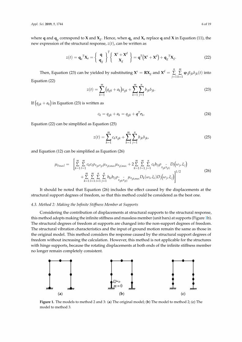
4.3. Method 2: Making the Infinite Stiffness Member at Supports
Considering the contribution of displacements at structural supports to the structural response,this method adopts making the infinite stiffness and massless member (unit bars) at supports (Figure 1b).The structural degrees of freedom at supports are changed into the non-support degrees of freedom.The structural vibration characteristics and the input of ground motion remain the same as those inthe original model. This method considers the response caused by the structural support degrees offreedom without increasing the calculation. However, this method is not applicable for the structureswith hinge supports, because the rotating displacements at both ends of the infinite stiffness memberno longer remain completely consistent.
Appl. Sci. 2019, 9, x FOR PEER REVIEW 7 of 20
the same as those in the original model. This method considers the response caused by the structural support degrees of freedom without increasing the calculation. However, this method is not applicable for the structures with hinge supports, because the rotating displacements at both ends of the infinite stiffness member no longer remain completely consistent.
4.4. Method 3: increasing the degrees of freedom around structural supports
This method is used to increase the degrees of freedom around structural supports (Figure 1 (c)). All or almost all contributions of the displacements at the structural supports to the structural response coul
(a)
_0m =
(b) (c)
Figure 1. The models to method 2 and 3: (a) The original model; (b) The model to method 2; (c) The model to method 3.
5. The verification of the modified MSRS method
Here, a five-span reinforced concrete bridge is modeled as a 2-D frame system shown in Figure 2, which is used to verify the modified MSRS method in comparison with the original MSRS method. The distributions of the bridge mass and stiffness are homogeneous. Each span is 60 m and the width of the main bridge is 10 m. The girder consists of four single-box pre-stressed concrete continuous box girders, as shown in Figure 3. The four main piers are rectangular reinforced concrete piers with the same cross sections of 1.8 m × 2.4 m, the same heights of 18.0 m, and the same damping radios of ξ1 = ξ2 = 0.02.
60 60 60 60 60 .
Figure 2. The five-span continuous rigid frame bridge (unit: m).
0.71.8
10
1.6
1.2
Figure 3. The girder’s cross section (unit: m).
The planar discrete model of the bridge used for calculating the structural responses is shown in Figure 4.
10 11 12 13 14 15 16 17 18 19 20 21 22 23 24 25 26 27 28 29 30 31
32
36
33
37
34
38
35
39
18
60 60 60 60 60
1 2 3 4 5 6 7 8 9
Figure 1. The models to method 2 and 3: (a) The original model; (b) The model to method 2; (c) Themodel to method 3.
Appl. Sci. 2019, 9, 1744 7 of 19
4.4. Method 3: Increasing the Degrees of Freedom around Structural Supports
This method is used to increase the degrees of freedom around structural supports (Figure 1c).All or almost all contributions of the displacements at the structural supports to the structural responsecould be substituted by the degrees of freedom near the supports. However, this method could resultin an obvious increase of computation.
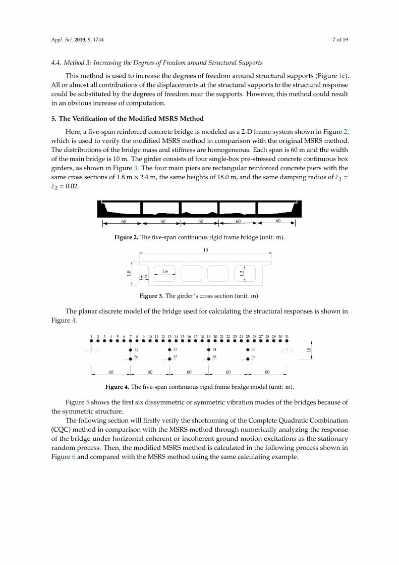
5. The Verification of the Modified MSRS Method
Here, a five-span reinforced concrete bridge is modeled as a 2-D frame system shown in Figure 2,which is used to verify the modified MSRS method in comparison with the original MSRS method.The distributions of the bridge mass and stiffness are homogeneous. Each span is 60 m and the widthof the main bridge is 10 m. The girder consists of four single-box pre-stressed concrete continuous boxgirders, as shown in Figure 3. The four main piers are rectangular reinforced concrete piers with thesame cross sections of 1.8 m × 2.4 m, the same heights of 18.0 m, and the same damping radios of ξ1 =
ξ2 = 0.02.
Appl. Sci. 2019, 9, x FOR PEER REVIEW 7 of 20
the same as those in the original model. This method considers the response caused by the structural support degrees of freedom without increasing the calculation. However, this method is not applicable for the structures with hinge supports, because the rotating displacements at both ends of the infinite stiffness member no longer remain completely consistent.
4.4. Method 3: increasing the degrees of freedom around structural supports
This method is used to increase the degrees of freedom around structural supports (Figure 1 (c)). All or almost all contributions of the displacements at the structural supports to the structural response could be substituted by the degrees of freedom near the supports. However, this method could result in an obvious increase of computation.
(a)
_0m =
(b)
(c)
Figure 1. The models to method 2 and 3: (a) The original model; (b) The model to method 2; (c) The model to method 3.
5. The verification of the modified MSRS method
Here, a five-span reinforced concrete bridge is modeled as a 2-D frame system shown in Figure 2, which is used to verify the modified MSRS method in comparison with the original MSRS method. The distributions of the bridge mass and stiffness are homogeneous. Each span is 60 m and the width of the main bridge is 10 m. The girder consists of four single-box pre-stressed concrete continuous box girders, as shown in Figure 3. The four main piers are rectangular reinforced concrete piers with the same cross sections of 1.8 m × 2.4 m, the same heights of 18.0 m, and the same damping radios of ξ1 = ξ2 = 0.02.
60 60 60 60 60 .
Figure 2. The five-span continuous rigid frame bridge (unit: m).
0.71.8
10
1.6
1.2
Figure 3. The girder’s cross section (unit: m).
The planar discrete model of the bridge used for calculating the structural responses is shown in Figure 4.
10 11 12 13 14 15 16 17 18 19 20 21 22 23 24 25 26 27 28 29 30 31
32
36
33
37
34
38
35
39
18
60 60 60 60 60
1 2 3 4 5 6 7 8 9
Figure 2. The five-span continuous rigid frame bridge (unit: m).
Appl. Sci. 2019, 9, x FOR PEER REVIEW 7 of 20
the same as those in the original model. This method considers the response caused by the structural support degrees of freedom without increasing the calculation. However, this method is not applicable for the structures with hinge supports, because the rotating displacements at both ends of the infinite stiffness member no longer remain completely consistent.
4.4. Method 3: increasing the degrees of freedom around structural supports
This method is used to increase the degrees of freedom around structural supports (Figure 1 (c)). All or almost all contributions of the displacements at the structural supports to the structural response could be substituted by the degrees of freedom near the supports. However, this method could result in an obvious increase of computation.
(a)
_0m =
(b)
(c)
Figure 1. The models to method 2 and 3: (a) The original model; (b) The model to method 2; (c) The model to method 3.
5. The verification of the modified MSRS method
Here, a five-span reinforced concrete bridge is modeled as a 2-D frame system shown in Figure 2, which is used to verify the modified MSRS method in comparison with the original MSRS method. The distributions of the bridge mass and stiffness are homogeneous. Each span is 60 m and the width of the main bridge is 10 m. The girder consists of four single-box pre-stressed concrete continuous box girders, as shown in Figure 3. The four main piers are rectangular reinforced concrete piers with the same cross sections of 1.8 m × 2.4 m, the same heights of 18.0 m, and the same damping radios of ξ1 = ξ2 = 0.02.
60 60 60 60 60 .
Figure 2. The five-span continuous rigid frame bridge (unit: m).
0.71.8
10
1.6
1.2
Figure 3. The girder’s cross section (unit: m).
The planar discrete model of the bridge used for calculating the structural responses is shown in Figure 4.
10 11 12 13 14 15 16 17 18 19 20 21 22 23 24 25 26 27 28 29 30 31
32
36
33
37
34
38
35
39
18
60 60 60 60 60
1 2 3 4 5 6 7 8 9
Figure 3. The girder’s cross section (unit: m).
The planar discrete model of the bridge used for calculating the structural responses is shown inFigure 4.
Appl. Sci. 2019, 9, x FOR PEER REVIEW 7 of 20
the same as those in the original model. This method considers the response caused by the structural support degrees of freedom without increasing the calculation. However, this method is not applicable for the structures with hinge supports, because the rotating displacements at both ends of the infinite stiffness member no longer remain completely consistent.
4.4. Method 3: increasing the degrees of freedom around structural supports
This method is used to increase the degrees of freedom around structural supports (Figure 1 (c)). All or almost all contributions of the displacements at the structural supports to the structural response could be substituted by the degrees of freedom near the supports. However, this method could result in an obvious increase of computation.
(a)
_0m =
(b)
(c)
Figure 1. The models to method 2 and 3: (a) The original model; (b) The model to method 2; (c) The model to method 3.
5. The verification of the modified MSRS method
Here, a five-span reinforced concrete bridge is modeled as a 2-D frame system shown in Figure 2, which is used to verify the modified MSRS method in comparison with the original MSRS method. The distributions of the bridge mass and stiffness are homogeneous. Each span is 60 m and the width of the main bridge is 10 m. The girder consists of four single-box pre-stressed concrete continuous box girders, as shown in Figure 3. The four main piers are rectangular reinforced concrete piers with the same cross sections of 1.8 m × 2.4 m, the same heights of 18.0 m, and the same damping radios of ξ1 = ξ2 = 0.02.
60 60 60 60 60 .
Figure 2. The five-span continuous rigid frame bridge (unit: m).
0.71.8
10
1.6
1.2
Figure 3. The girder’s cross section (unit: m).
The planar discrete model of the bridge used for calculating the structural responses is shown in Figure 4.
10 11 12 13 14 15 16 17 18 19 20 21 22 23 24 25 26 27 28 29 30 31
32
36
33
37
34
38
35
39
18
60 60 60 60 60
1 2 3 4 5 6 7 8 9
Figure 4. The five-span continuous rigid frame bridge model (unit: m).
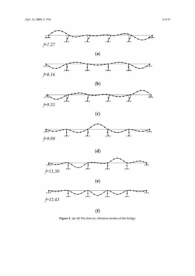
Figure 5 shows the first six dissymmetric or symmetric vibration modes of the bridges because ofthe symmetric structure.
The following section will firstly verify the shortcoming of the Complete Quadratic Combination(CQC) method in comparison with the MSRS method through numerically analyzing the responseof the bridge under horizontal coherent or incoherent ground motion excitations as the stationaryrandom process. Then, the modified MSRS method is calculated in the following process shown inFigure 6 and compared with the MSRS method using the same calculating example.
Appl. Sci. 2019, 9, 1744 8 of 19
Appl. Sci. 2019, 9, x FOR PEER REVIEW 8 of 20
Figure 4. The five-span continuous rigid frame bridge model (unit: m).
Figure 5 shows the first six dissymmetric or symmetric vibration modes of the bridges because of the symmetric structure.
f=7.27 (a)
f=8.16 (b)
f=9.31 (c)
f=9.98
(d)
f=11.30
(e)
f=12.43
(f)
Figure 5. (a)–(f) The first six vibration modes of the bridge. Figure 5. (a)–(f) The first six vibration modes of the bridge.
Appl. Sci. 2019, 9, 1744 9 of 19
Appl. Sci. 2019, 9, x FOR PEER REVIEW 9 of 20
Judge the degree of structured freedom
Achieve the vibration modes and natural frequencies
Calculate the structure response
Decouple through Matrix decomposition
Method 1Make the structural
displacement vector
Method 2Make the infinite
stiffness member at supportsMethod 3
Increase the degrees of freedom around structural
supports
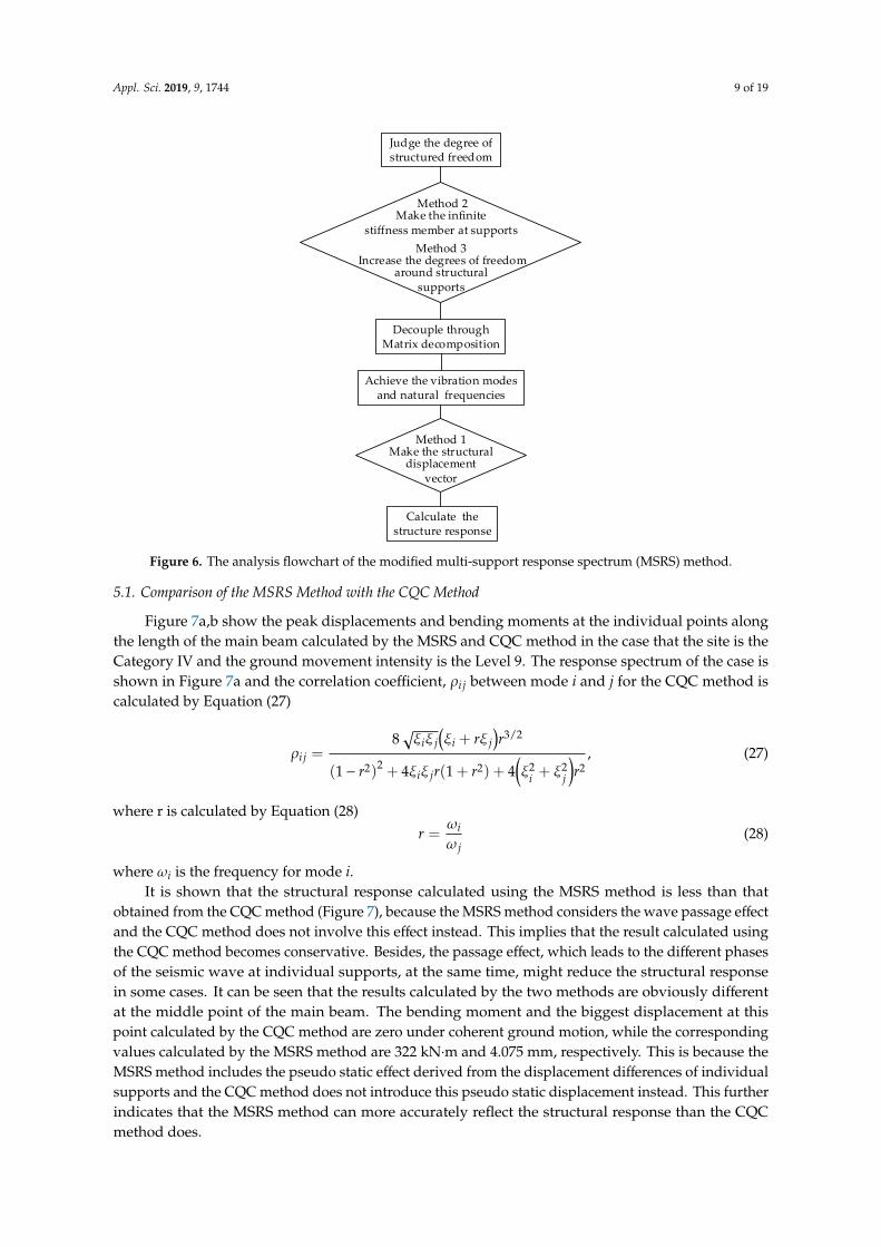
Figure 6. The analysis flowchart of the modified multi-support response spectrum (MSRS) method.
The following section will firstly verify the shortcoming of the Complete Quadratic Combination (CQC) method in comparison with the MSRS method through numerically analyzing the response of the bridge under horizontal coherent or incoherent ground motion excitations as the stationary random process. Then, the modified MSRS method is calculated in the following process shown in Figure 6 and compared with the MSRS method using the same calculating example.
5.1. Comparison of the MSRS method with the CQC method
Figures 7(a) and (b) show the peak displacements and bending moments at the individual points along the length of the main beam calculated by the MSRS and CQC method in the case that the site is the Category IV and the ground movement intensity is the Level 9. The response spectrum of the case is shown in Figure 7(a) and the correlation coefficient, ijρ between mode i and j for the CQC method is calculated by Equation (27)
( )( ) ( ) ( )
3 2
22 2 2 2 2
8
1 4 1 4i j i j
ij
i j i j
r r
r r r r
ξ ξ ξ ξρ
ξ ξ ξ ξ
+=
− + + + +, (27)
where r is calculated by Equation (28)
i
j
rωω
= , (15)
where iω is the frequency for mode i. It is shown that the structural response calculated using the MSRS method is less than that
obtained from the CQC method (Figure 7), because the MSRS method considers the wave passage effect and the CQC method does not involve this effect instead. This implies that the result calculated using the CQC method becomes conservative. Besides, the passage effect, which leads to the different phases of the seismic wave at individual supports, at the same time, might reduce the structural response in some cases. It can be seen that the results calculated by the two methods are obviously different at the middle point of the main beam. The bending moment and the biggest displacement at this point calculated by the CQC method are zero under coherent ground motion,
Figure 6. The analysis flowchart of the modified multi-support response spectrum (MSRS) method.
5.1. Comparison of the MSRS Method with the CQC Method
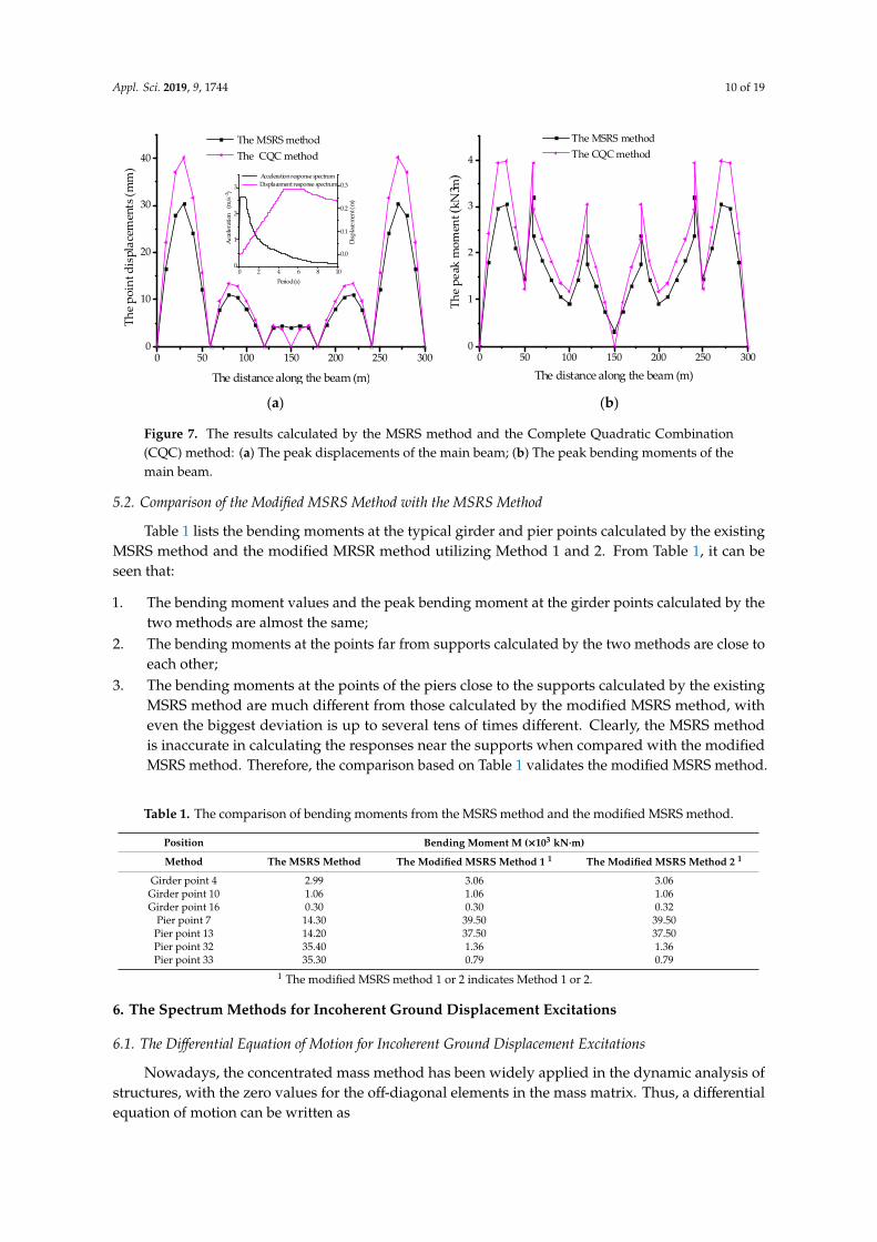
Figure 7a,b show the peak displacements and bending moments at the individual points alongthe length of the main beam calculated by the MSRS and CQC method in the case that the site is theCategory IV and the ground movement intensity is the Level 9. The response spectrum of the case isshown in Figure 7a and the correlation coefficient, ρi j between mode i and j for the CQC method iscalculated by Equation (27)
ρi j =8√ξiξ j
(ξi + rξ j
)r3/2
(1− r2)2 + 4ξiξ jr(1 + r2) + 4(ξ2
i + ξ2j
)r2
, (27)
where r is calculated by Equation (28)r =
ωiω j
(28)
where ωi is the frequency for mode i.It is shown that the structural response calculated using the MSRS method is less than that
obtained from the CQC method (Figure 7), because the MSRS method considers the wave passage effectand the CQC method does not involve this effect instead. This implies that the result calculated usingthe CQC method becomes conservative. Besides, the passage effect, which leads to the different phasesof the seismic wave at individual supports, at the same time, might reduce the structural responsein some cases. It can be seen that the results calculated by the two methods are obviously differentat the middle point of the main beam. The bending moment and the biggest displacement at thispoint calculated by the CQC method are zero under coherent ground motion, while the correspondingvalues calculated by the MSRS method are 322 kN·m and 4.075 mm, respectively. This is because theMSRS method includes the pseudo static effect derived from the displacement differences of individualsupports and the CQC method does not introduce this pseudo static displacement instead. This furtherindicates that the MSRS method can more accurately reflect the structural response than the CQCmethod does.
Appl. Sci. 2019, 9, 1744 10 of 19
Appl. Sci. 2019, 9, x FOR PEER REVIEW 10 of 20
while the corresponding values calculated by the MSRS method are 322 kN∙m and 4.075 mm, respectively. This is because the MSRS method includes the pseudo static effect derived from the displacement differences of individual supports and the CQC method does not introduce this pseudo static displacement instead. This further indicates that the MSRS method can more accurately reflect the structural response than the CQC method does.
0 50 100 150 200 250 3000
10
20
30
40
0 2 4 6 8 100
1
2
3
Acc
eler
atio
n (m
/s-2
)
Period (s)
Acceleration response spectrum
0.0
0.1
0.2
0.3 Displacement response spectrum
Disp
lace
men
t (m
)
The MSRS method The CQC method
The p
oint
dis
plac
emen
ts (m
m)
The distance along the beam (m)
(a)
0 50 100 150 200 250 3000
1
2
3
4
The
peak
mom
ent (
kN3m
)
The distance along the beam (m)
The MSRS method The CQC method
(b)
Figure 7. The results calculated by the MSRS method and the Complete Quadratic Combination (CQC) method: (a) The peak displacements of the main beam; (b) The peak bending moments of the main beam.
5.2. Comparison of the modified MSRS method with the MSRS method
Table 1 lists the bending moments at the typical girder and pier points calculated by the existing MSRS method and the modified MRSR method utilizing Method 1 and 2. From Table 1, it can be seen that: 1. The bending moment values and the peak bending moment at the girder points calculated by
the two methods are almost the same; 2. The bending moments at the points far from supports calculated by the two methods are close
to each other; 3. The bending moments at the points of the piers close to the supports calculated by the existing
MSRS method are much different from those calculated by the modified MSRS method, with even the biggest deviation is up to several tens of times different. Clearly, the MSRS method is inaccurate in calculating the responses near the supports when compared with the modified MSRS method. Therefore, the comparison based on Table 1 validates the modified MSRS method.
Table 1. The comparison of bending moments from the MSRS method and the modified MSRS method.
Position Bending moment M (×103 kN∙m)
Method The MSRS method The modified MSRS method 1 1
The modified MSRS method 2 1
Girder point 4 2.99 3.06 3.06 Girder point 10 1.06 1.06 1.06 Girder point 16 0.30 0.30 0.32
Pier point 7 14.30 39.50 39.50 Pier point 13 14.20 37.50 37.50 Pier point 32 35.40 1.36 1.36 Pier point 33 35.30 0.79 0.79
1 The modified MSRS method 1 or 2 indicates Method 1 or 2.
Figure 7. The results calculated by the MSRS method and the Complete Quadratic Combination(CQC) method: (a) The peak displacements of the main beam; (b) The peak bending moments of themain beam.
5.2. Comparison of the Modified MSRS Method with the MSRS Method
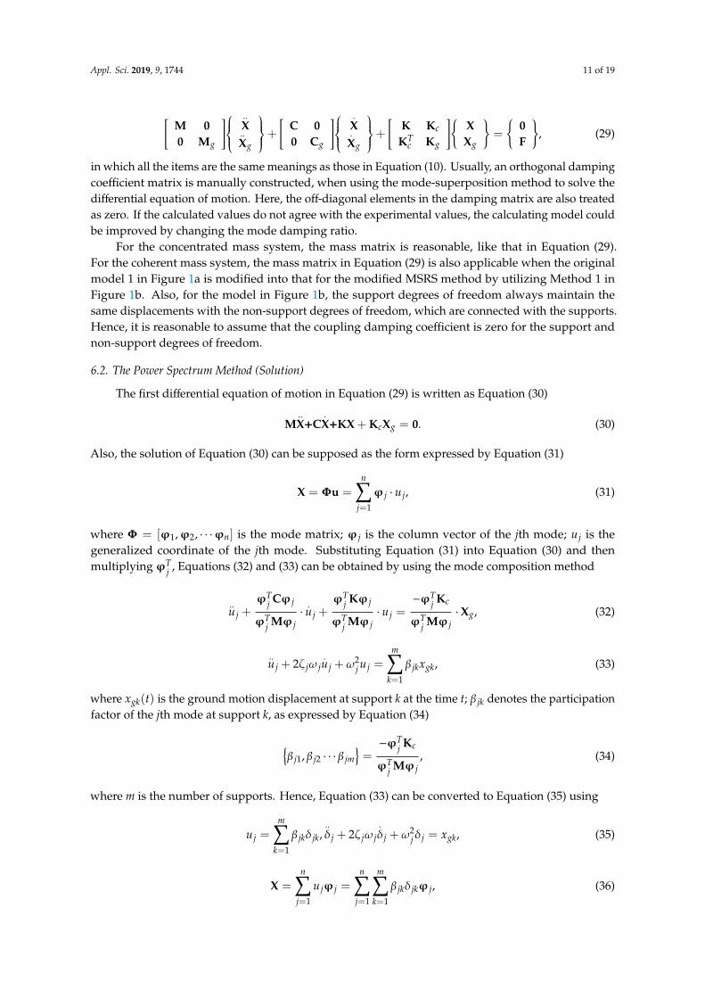
Table 1 lists the bending moments at the typical girder and pier points calculated by the existingMSRS method and the modified MRSR method utilizing Method 1 and 2. From Table 1, it can beseen that:
1. The bending moment values and the peak bending moment at the girder points calculated by thetwo methods are almost the same;
2. The bending moments at the points far from supports calculated by the two methods are close toeach other;
3. The bending moments at the points of the piers close to the supports calculated by the existingMSRS method are much different from those calculated by the modified MSRS method, witheven the biggest deviation is up to several tens of times different. Clearly, the MSRS methodis inaccurate in calculating the responses near the supports when compared with the modifiedMSRS method. Therefore, the comparison based on Table 1 validates the modified MSRS method.
Table 1. The comparison of bending moments from the MSRS method and the modified MSRS method.
Position Bending Moment M (×103 kN·m)
Method The MSRS Method The Modified MSRS Method 1 1 The Modified MSRS Method 2 1
Girder point 4 2.99 3.06 3.06Girder point 10 1.06 1.06 1.06Girder point 16 0.30 0.30 0.32
Pier point 7 14.30 39.50 39.50Pier point 13 14.20 37.50 37.50Pier point 32 35.40 1.36 1.36Pier point 33 35.30 0.79 0.79
1 The modified MSRS method 1 or 2 indicates Method 1 or 2.
6. The Spectrum Methods for Incoherent Ground Displacement Excitations
6.1. The Differential Equation of Motion for Incoherent Ground Displacement Excitations
Nowadays, the concentrated mass method has been widely applied in the dynamic analysis ofstructures, with the zero values for the off-diagonal elements in the mass matrix. Thus, a differentialequation of motion can be written as
Appl. Sci. 2019, 9, 1744 11 of 19
[M 00 Mg
]..X..Xg
+
[C 00 Cg
].X.Xg
+
[K Kc
KTc Kg
]{XXg
}=
{0F
}, (29)
in which all the items are the same meanings as those in Equation (10). Usually, an orthogonal dampingcoefficient matrix is manually constructed, when using the mode-superposition method to solve thedifferential equation of motion. Here, the off-diagonal elements in the damping matrix are also treatedas zero. If the calculated values do not agree with the experimental values, the calculating model couldbe improved by changing the mode damping ratio.
For the concentrated mass system, the mass matrix is reasonable, like that in Equation (29).For the coherent mass system, the mass matrix in Equation (29) is also applicable when the originalmodel 1 in Figure 1a is modified into that for the modified MSRS method by utilizing Method 1 inFigure 1b. Also, for the model in Figure 1b, the support degrees of freedom always maintain thesame displacements with the non-support degrees of freedom, which are connected with the supports.Hence, it is reasonable to assume that the coupling damping coefficient is zero for the support andnon-support degrees of freedom.
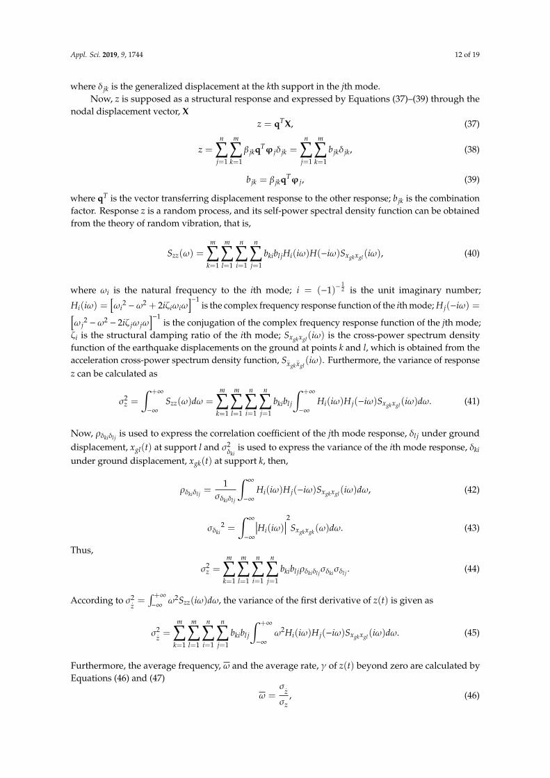
6.2. The Power Spectrum Method (Solution)
The first differential equation of motion in Equation (29) is written as Equation (30)
M..X+C
.X+KX + KcXg = 0. (30)
Also, the solution of Equation (30) can be supposed as the form expressed by Equation (31)
X = Φu =n∑
j=1
ϕ j · u j, (31)
where Φ = [ϕ1,ϕ2, · · ·ϕn] is the mode matrix; ϕ j is the column vector of the jth mode; u j is thegeneralized coordinate of the jth mode. Substituting Equation (31) into Equation (30) and thenmultiplying ϕT
j , Equations (32) and (33) can be obtained by using the mode composition method
..u j +
ϕTj Cϕ j
ϕTj Mϕ j
·.u j +
ϕTj Kϕ j
ϕTj Mϕ j
· u j =−ϕT
j Kc
ϕTj Mϕ j
·Xg, (32)
..u j + 2ζ jω j
.u j +ω2
j u j =m∑
k=1
β jkxgk, (33)
where xgk(t) is the ground motion displacement at support k at the time t; β jk denotes the participationfactor of the jth mode at support k, as expressed by Equation (34)
{β j1, β j2 · · · β jm
}=−ϕT
j Kc
ϕTj Mϕ j
, (34)
where m is the number of supports. Hence, Equation (33) can be converted to Equation (35) using
u j =m∑
k=1
β jkδ jk,..δ j + 2ζ jω j
.δ j +ω2
jδ j = xgk, (35)
X =n∑
j=1
u jϕ j =n∑
j=1
m∑k=1
β jkδ jkϕ j, (36)
Appl. Sci. 2019, 9, 1744 12 of 19
where δ jk is the generalized displacement at the kth support in the jth mode.Now, z is supposed as a structural response and expressed by Equations (37)–(39) through the
nodal displacement vector, Xz = qTX, (37)
z =n∑
j=1
m∑k=1
β jkqTϕ jδ jk =n∑
j=1
m∑k=1
b jkδ jk, (38)
b jk = β jkqTϕ j, (39)
where qT is the vector transferring displacement response to the other response; b jk is the combinationfactor. Response z is a random process, and its self-power spectral density function can be obtainedfrom the theory of random vibration, that is,
Szz(ω) =m∑
k=1
m∑l=1
n∑i=1
n∑j=1
bkibl jHi(iω)H(−iω)Sxgkxgl(iω), (40)
where ωi is the natural frequency to the ith mode; i = (−1)−12 is the unit imaginary number;
Hi(iω) =[ωi
2−ω2 + 2iζiωiω
]−1is the complex frequency response function of the ith mode; H j(−iω) =[
ω j2−ω2
− 2iζ jω jω]−1
is the conjugation of the complex frequency response function of the jth mode;ζi is the structural damping ratio of the ith mode; Sxgkxgl(iω) is the cross-power spectrum densityfunction of the earthquake displacements on the ground at points k and l, which is obtained from theacceleration cross-power spectrum density function, S..
xgk..xgl(iω). Furthermore, the variance of response
z can be calculated as
σ2z =
∫ +∞
−∞
Szz(ω)dω =m∑
k=1
m∑l=1
n∑i=1
n∑j=1
bkibl j
∫ +∞
−∞
Hi(iω)H j(−iω)Sxgkxgl(iω)dω. (41)
Now, ρδkiδl j is used to express the correlation coefficient of the jth mode response, δl j under grounddisplacement, xgl(t) at support l and σ2
δkiis used to express the variance of the ith mode response, δki
under ground displacement, xgk(t) at support k, then,
ρδkiδl j =1
σδkiδl j
∫∞
−∞
Hi(iω)H j(−iω)Sxgkxgl(iω)dω, (42)
σδki2 =
∫∞
−∞
∣∣∣Hi(iω)∣∣∣2Sxgkxgk(ω)dω. (43)
Thus,
σ2z =
m∑k=1
m∑l=1
n∑i=1
n∑j=1
bkibl jρδkiδl jσδkiσδl j . (44)
According to σ2.z=
∫ +∞
−∞ω2Szz(iω)dω, the variance of the first derivative of z(t) is given as
σ2.z=
m∑k=1
m∑l=1
n∑i=1
n∑j=1
bkibl j
∫ +∞
−∞
ω2Hi(iω)H j(−iω)Sxgkxgl(iω)dω. (45)
Furthermore, the average frequency, ω and the average rate, γ of z(t) beyond zero are calculated byEquations (46) and (47)
ω =σ .
zσz
, (46)
Appl. Sci. 2019, 9, 1744 13 of 19
γ =ωπ
. (47)
Meanwhile, the peak response factors, pz and qz of z(t) can be calculated by Equations (48) and (49)
pz =√
2 ln(γTd) +0.5772√2 ln(γTd)
, (48)
qz =π√
6
1√2 ln(γTd)
, (49)
where Td is the duration of an earthquake.Finally, the mean value and mean value square deviation of the absolute peak value, |zmax| for the
structural response, z(t) during the period, [0, Td] can be obtained as
µ|zmax | = pzσz, (50)
σ|zmax | = qzσz. (51)
Once µ|zmax | and σ|zmax | are determined, the mean and variance of the peak response of the structure canbe obtained.
6.3. The Response Spectrum Method for Incoherent Ground Displacement Excitations
By substituting Equation (45) into Equation (46), µzmax can be written as
µzmax =
m∑k=1
m∑l=1
n∑i=1
n∑j=1
bkibl jρδkiδl j p2zσδkiσδl j
12
. (52)
According to the definition of the response spectrum, a response spectrum value equals to averageresponse of a single degree-of-freedom system subjected to the same ground excitation. Hence,
Dk(ωi, ζi) = pδkiσδki . (53)
Substituting Equation (53) into Equation (52), µzmax can be written as
µzmax =
m∑k=1
m∑l=1
n∑i=1
n∑j=1
bkibl jρδkiδl j
p2z
pδki pδl j
Dk(ωi, ζi)Dl(ω j, ζ j
)12
. (54)
Because p2z/
(pδki pδl j
)is near to 1, then
µzmax =
m∑k=1
m∑l=1
n∑i=1
n∑j=1
bkibl jρδkiδl jDk(ωi, ζi)Dl(ω j, ζ j
)12
. (55)
Equation (55) is the expression of the mean of the structural peak response under incoherent grounddisplacement excitation.
In consideration of the effect of the support degrees of freedom, the expression of the meanresponse spectrum method should be modified. Therefore, a structural response, z(t) can be expressedby the nodal displacement, Xa and qa,
z(t) = qaTXa =
{qqg
}T{XXg
}= qTX + qg
TXg, (56)
Appl. Sci. 2019, 9, 1744 14 of 19
z(t) =m∑
k=1
qgkxgk(t) +n∑
j=1
m∑k=1
β jkqTϕ jδ jk(t) =m∑
k=1
qgkxgk(t) +n∑
j=1
m∑k=1
b jkδ jk(t), (57)
µ|z,max| =
m∑k=1
m∑l=1
qgkqglρxgkxglµxgk,maxµxgl,max + 2m∑
k=1
m∑l=1
n∑j=1
qgkbl jρxgk”xl j
Dl(ω j, ζ j
)+
m∑k=1
m∑l=1
n∑i=1
n∑j=1
bkibl jρ”xgki
”xgljµxgk,maxDk(ωi, ζi)Dl
(ω j, ζ j
)12
(58)
where qgk is the conversion factor of xgk in the conversion vector, qT.It should be noted that the structural response derived from Equations (57) and (58) needs to
be used to construct the structural displacement vector, Xa like the modified MSRS method utilizingMethod 1.
6.4. The Simplified Power Spectrum Method
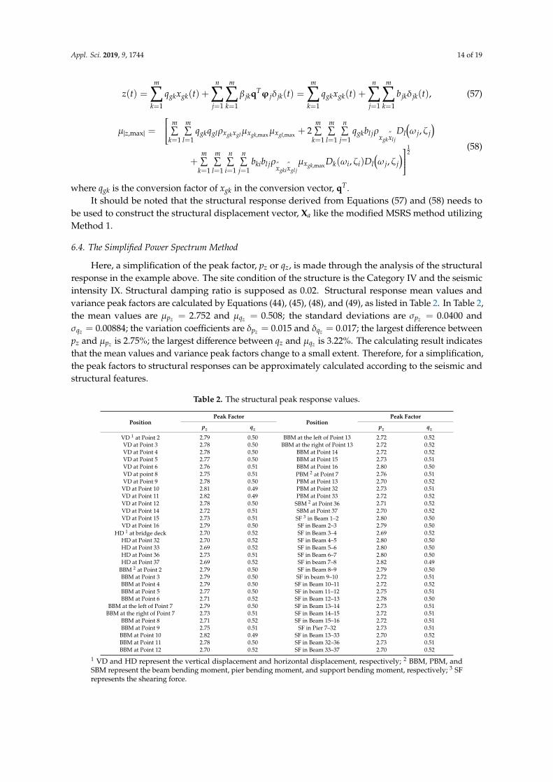
Here, a simplification of the peak factor, pz or qz, is made through the analysis of the structuralresponse in the example above. The site condition of the structure is the Category IV and the seismicintensity IX. Structural damping ratio is supposed as 0.02. Structural response mean values andvariance peak factors are calculated by Equations (44), (45), (48), and (49), as listed in Table 2. In Table 2,the mean values are µpz = 2.752 and µqz = 0.508; the standard deviations are σpz = 0.0400 andσqz = 0.00884; the variation coefficients are δpz = 0.015 and δqz = 0.017; the largest difference betweenpz and µpz is 2.75%; the largest difference between qz and µqz is 3.22%. The calculating result indicatesthat the mean values and variance peak factors change to a small extent. Therefore, for a simplification,the peak factors to structural responses can be approximately calculated according to the seismic andstructural features.
Table 2. The structural peak response values.
PositionPeak Factor
PositionPeak Factor
pz qz pz qz
VD 1 at Point 2 2.79 0.50 BBM at the left of Point 13 2.72 0.52VD at Point 3 2.78 0.50 BBM at the right of Point 13 2.72 0.52VD at Point 4 2.78 0.50 BBM at Point 14 2.72 0.52VD at Point 5 2.77 0.50 BBM at Point 15 2.73 0.51VD at Point 6 2.76 0.51 BBM at Point 16 2.80 0.50VD at point 8 2.75 0.51 PBM 2 at Point 7 2.76 0.51VD at Point 9 2.78 0.50 PBM at Point 13 2.70 0.52
VD at Point 10 2.81 0.49 PBM at Point 32 2.73 0.51VD at Point 11 2.82 0.49 PBM at Point 33 2.72 0.52VD at Point 12 2.78 0.50 SBM 2 at Point 36 2.71 0.52VD at Point 14 2.72 0.51 SBM at Point 37 2.70 0.52VD at Point 15 2.73 0.51 SF 3 in Beam 1–2 2.80 0.50VD at Point 16 2.79 0.50 SF in Beam 2–3 2.79 0.50
HD 1 at bridge deck 2.70 0.52 SF in Beam 3–4 2.69 0.52HD at Point 32 2.70 0.52 SF in Beam 4–5 2.80 0.50HD at Point 33 2.69 0.52 SF in Beam 5–6 2.80 0.50HD at Point 36 2.73 0.51 SF in Beam 6–7 2.80 0.50HD at Point 37 2.69 0.52 SF in beam 7–8 2.82 0.49
BBM 2 at Point 2 2.79 0.50 SF in Beam 8–9 2.79 0.50BBM at Point 3 2.79 0.50 SF in beam 9–10 2.72 0.51BBM at Point 4 2.79 0.50 SF in Beam 10–11 2.72 0.52BBM at Point 5 2.77 0.50 SF in beam 11–12 2.75 0.51BBM at Point 6 2.71 0.52 SF in Beam 12–13 2.78 0.50
BBM at the left of Point 7 2.79 0.50 SF in Beam 13–14 2.73 0.51BBM at the right of Point 7 2.73 0.51 SF in Beam 14–15 2.72 0.51
BBM at Point 8 2.71 0.52 SF in Beam 15–16 2.72 0.51BBM at Point 9 2.75 0.51 SF in Pier 7–32 2.73 0.51
BBM at Point 10 2.82 0.49 SF in Beam 13–33 2.70 0.52BBM at Point 11 2.78 0.50 SF in Beam 32–36 2.73 0.51BBM at Point 12 2.70 0.52 SF in Beam 33–37 2.70 0.52
1 VD and HD represent the vertical displacement and horizontal displacement, respectively; 2 BBM, PBM, andSBM represent the beam bending moment, pier bending moment, and support bending moment, respectively; 3 SFrepresents the shearing force.
Appl. Sci. 2019, 9, 1744 15 of 19
The mean value, pg and the peak variance factor, qg of ground motion displacement can becalculated by substituting Equations (59) and (60) into Equations (48), (49), (50), and (51)
λm =
∫∞
−∞
ωmS(ω)dω, (59)
ω =
√λ2√λ0
. (60)
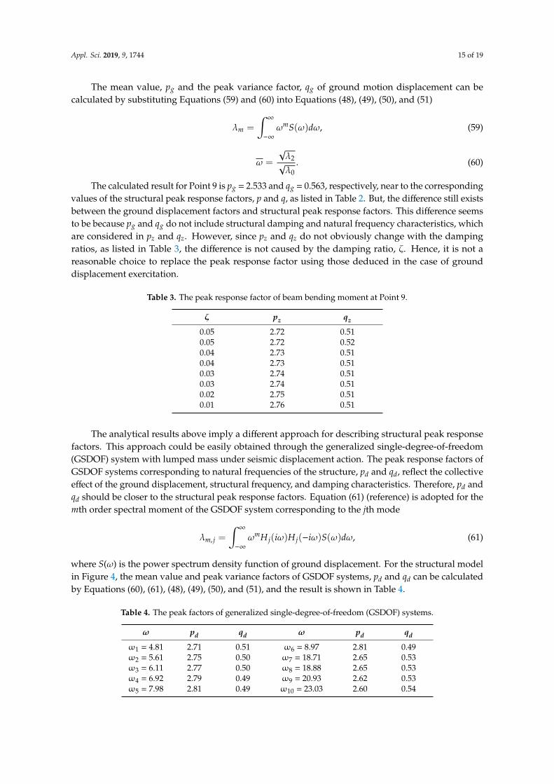
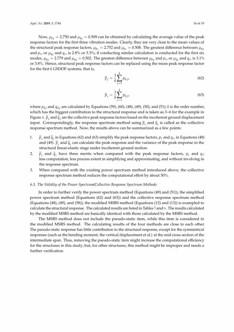
The calculated result for Point 9 is pg = 2.533 and qg = 0.563, respectively, near to the correspondingvalues of the structural peak response factors, p and q, as listed in Table 2. But, the difference still existsbetween the ground displacement factors and structural peak response factors. This difference seemsto be because pg and qg do not include structural damping and natural frequency characteristics, whichare considered in pz and qz. However, since pz and qz do not obviously change with the dampingratios, as listed in Table 3, the difference is not caused by the damping ratio, ζ. Hence, it is not areasonable choice to replace the peak response factor using those deduced in the case of grounddisplacement exercitation.
Table 3. The peak response factor of beam bending moment at Point 9.
ζ pz qz
0.05 2.72 0.510.05 2.72 0.520.04 2.73 0.510.04 2.73 0.510.03 2.74 0.510.03 2.74 0.510.02 2.75 0.510.01 2.76 0.51
The analytical results above imply a different approach for describing structural peak responsefactors. This approach could be easily obtained through the generalized single-degree-of-freedom(GSDOF) system with lumped mass under seismic displacement action. The peak response factors ofGSDOF systems corresponding to natural frequencies of the structure, pd and qd, reflect the collectiveeffect of the ground displacement, structural frequency, and damping characteristics. Therefore, pd andqd should be closer to the structural peak response factors. Equation (61) (reference) is adopted for themth order spectral moment of the GSDOF system corresponding to the jth mode
λm, j =
∫∞
−∞
ωmH j(iω)H j(−iω)S(ω)dω, (61)
where S(ω) is the power spectrum density function of ground displacement. For the structural modelin Figure 4, the mean value and peak variance factors of GSDOF systems, pd and qd can be calculatedby Equations (60), (61), (48), (49), (50), and (51), and the result is shown in Table 4.
Table 4. The peak factors of generalized single-degree-of-freedom (GSDOF) systems.
ω pd qd ω pd qd
ω1 = 4.81 2.71 0.51 ω6 = 8.97 2.81 0.49ω2 = 5.61 2.75 0.50 ω7 = 18.71 2.65 0.53ω3 = 6.11 2.77 0.50 ω8 = 18.88 2.65 0.53ω4 = 6.92 2.79 0.49 ω9 = 20.93 2.62 0.53ω5 = 7.98 2.81 0.49 ω10 = 23.03 2.60 0.54
Appl. Sci. 2019, 9, 1744 16 of 19
Now, µpd = 2.750 and µqd = 0.509 can be obtained by calculating the average value of the peakresponse factors for the first three vibration modes. Clearly, they are very close to the mean values ofthe structural peak response factors, µpz = 2.752 and µqz = 0.508. The greatest difference between µpd
and pz, or µqd and qz, is 2.8% or 3.3%; if conducting similar calculation is conducted for the first sixmodes, µpd = 2.779 and µqd = 0.502. The greatest difference between µpd and pz, or µqd and qz, is 3.1%or 3.8%. Hence, structural peak response factors can be replaced using the mean peak response factorfor the first k GSDOF systems, that is,
pz =1k
k∑j=1
pd, j, (62)
pz =1k
k∑j=1
pd, j, (63)
where pd,j and qd,j are calculated by Equations (59), (60), (48), (49), (50), and (51); k is the order number,which has the biggest contribution to the structural response and is taken as 3~6 for the example inFigure 4. pz and qz are the collective peak response factors based on the incoherent ground displacementinput. Correspondingly, the response spectrum method using pz and qz is called as the collectiveresponse spectrum method. Now, the results above can be summarized as a few points:
1. pz and qz in Equations (62) and (63) simplify the peak response factors, pz and qz, in Equations (48)and (49). pz and qz can calculate the peak response and the variance of the peak response in thestructural linear-elastic stage under incoherent ground motion.
2. pz and qz have three merits when compared with the peak response factors, pz and qz:less computation, less process extent in simplifying and approximating, and without involving inthe response spectrum.
3. When compared with the existing power spectrum method introduced above, the collectiveresponse spectrum method reduces the computational effort by about 50%.
6.5. The Validity of the Power Spectrum/Collective Response Spectrum Methods
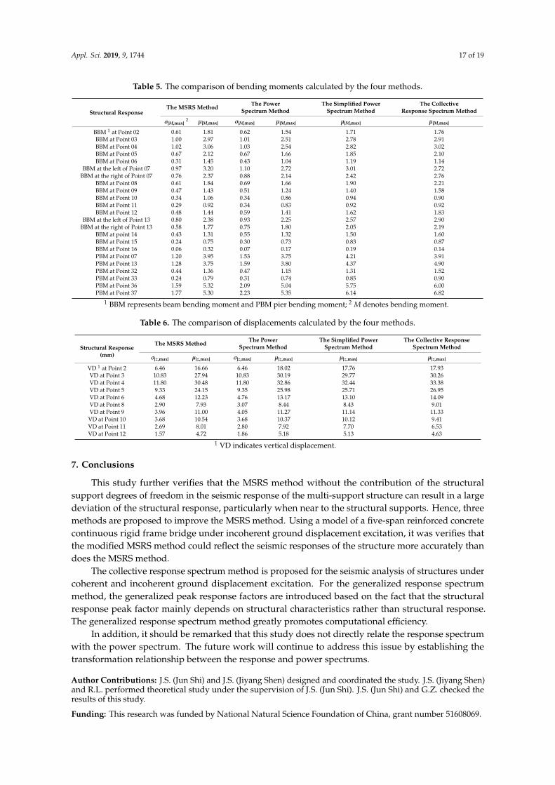
In order to further verify the power spectrum method (Equations (49) and (51)), the simplifiedpower spectrum method (Equations (62) and (63)) and the collective response spectrum method(Equations (48), (49), and (58)), the modified MSRS method (Equations (12) and (13)) is exampled tocalculate the structural response. The calculated results are listed in Tables 5 and 6. The results calculatedby the modified MSRS method are basically identical with those calculated by the MSRS method.
The MSRS method does not include the pseudo-static item, while this item is considered inthe modified MSRS method. The calculating results of the four methods are close to each other.The pseudo-static response has little contribution to the structural response, except for the symmetricalresponses (such as the bending moment, the vertical displacement et al.) at the mid-cross section of theintermediate span. Thus, removing the pseudo-static item might increase the computational efficiencyfor the structures in this study; but, for other structures, this method might be improper and needs afurther verification.
Appl. Sci. 2019, 9, 1744 17 of 19
Table 5. The comparison of bending moments calculated by the four methods.
Structural ResponseThe MSRS Method The Power
Spectrum MethodThe Simplified Power
Spectrum MethodThe Collective
Response Spectrum Method
σ|M,max|2 µ|M,max| σ|M,max| µ|M,max| µ|M,max| µ|M,max|
BBM 1 at Point 02 0.61 1.81 0.62 1.54 1.71 1.76BBM at Point 03 1.00 2.97 1.01 2.51 2.78 2.91BBM at Point 04 1.02 3.06 1.03 2.54 2.82 3.02BBM at Point 05 0.67 2.12 0.67 1.66 1.85 2.10BBM at Point 06 0.31 1.45 0.43 1.04 1.19 1.14
BBM at the left of Point 07 0.97 3.20 1.10 2.72 3.01 2.72BBM at the right of Point 07 0.76 2.37 0.88 2.14 2.42 2.76
BBM at Point 08 0.61 1.84 0.69 1.66 1.90 2.21BBM at Point 09 0.47 1.43 0.51 1.24 1.40 1.58BBM at Point 10 0.34 1.06 0.34 0.86 0.94 0.90BBM at Point 11 0.29 0.92 0.34 0.83 0.92 0.92BBM at Point 12 0.48 1.44 0.59 1.41 1.62 1.83
BBM at the left of Point 13 0.80 2.38 0.93 2.25 2.57 2.90BBM at the right of Point 13 0.58 1.77 0.75 1.80 2.05 2.19
BBM at point 14 0.43 1.31 0.55 1.32 1.50 1.60BBM at Point 15 0.24 0.75 0.30 0.73 0.83 0.87BBM at Point 16 0.06 0.32 0.07 0.17 0.19 0.14PBM at Point 07 1.20 3.95 1.53 3.75 4.21 3.91PBM at Point 13 1.28 3.75 1.59 3.80 4.37 4.90PBM at Point 32 0.44 1.36 0.47 1.15 1.31 1.52PBM at Point 33 0.24 0.79 0.31 0.74 0.85 0.90PBM at Point 36 1.59 5.32 2.09 5.04 5.75 6.00PBM at Point 37 1.77 5.30 2.23 5.35 6.14 6.82
1 BBM represents beam bending moment and PBM pier bending moment; 2 M denotes bending moment.
Table 6. The comparison of displacements calculated by the four methods.
Structural Response(mm)
The MSRS Method The PowerSpectrum Method
The Simplified PowerSpectrum Method
The Collective ResponseSpectrum Method
σ|z,max| µ|z,max| σ|z,max| µ|z,max| µ|z,max| µ|z,max|
VD 1 at Point 2 6.46 16.66 6.46 18.02 17.76 17.93VD at Point 3 10.83 27.94 10.83 30.19 29.77 30.26VD at Point 4 11.80 30.48 11.80 32.86 32.44 33.38VD at Point 5 9.33 24.15 9.35 25.98 25.71 26.95VD at Point 6 4.68 12.23 4.76 13.17 13.10 14.09VD at Point 8 2.90 7.93 3.07 8.44 8.43 9.01VD at Point 9 3.96 11.00 4.05 11.27 11.14 11.33VD at Point 10 3.68 10.54 3.68 10.37 10.12 9.41VD at Point 11 2.69 8.01 2.80 7.92 7.70 6.53VD at Point 12 1.57 4.72 1.86 5.18 5.13 4.63
1 VD indicates vertical displacement.
7. Conclusions
This study further verifies that the MSRS method without the contribution of the structuralsupport degrees of freedom in the seismic response of the multi-support structure can result in a largedeviation of the structural response, particularly when near to the structural supports. Hence, threemethods are proposed to improve the MSRS method. Using a model of a five-span reinforced concretecontinuous rigid frame bridge under incoherent ground displacement excitation, it was verifies thatthe modified MSRS method could reflect the seismic responses of the structure more accurately thandoes the MSRS method.
The collective response spectrum method is proposed for the seismic analysis of structures undercoherent and incoherent ground displacement excitation. For the generalized response spectrummethod, the generalized peak response factors are introduced based on the fact that the structuralresponse peak factor mainly depends on structural characteristics rather than structural response.The generalized response spectrum method greatly promotes computational efficiency.
In addition, it should be remarked that this study does not directly relate the response spectrumwith the power spectrum. The future work will continue to address this issue by establishing thetransformation relationship between the response and power spectrums.
Author Contributions: J.S. (Jun Shi) and J.S. (Jiyang Shen) designed and coordinated the study. J.S. (Jiyang Shen)and R.L. performed theoretical study under the supervision of J.S. (Jun Shi). J.S. (Jun Shi) and G.Z. checked theresults of this study.
Funding: This research was funded by National Natural Science Foundation of China, grant number 51608069.

Appl. Sci. 2019, 9, 1744 18 of 19
Acknowledgments: This research has been financially supported by National Natural Science Foundation ofChina (51608069). The authors would like to thank the members of the HIT 504 office for their selfless help anduseful suggestions.
Conflicts of Interest: The authors declare no conflict of interest
References
1. Andersen, M.S.; Brandt, A. Aerodynamic Instability Investigations of a Novel, Flexible and LightweightTriple-Box Girder Design for Long-Span Bridges. J. Bridge Eng. 2018, 23. [CrossRef]
2. Kamada, T.; Fujita, T. State of the Art of Development and Application of Antiseismic Systems in Japan.In Proceedings of the 2008 Seismic Engineering Conference: Commemorating the 1908 Messina and ReggioCalabria Earthquake, Reggio Calabria, Italy, 8–11 July 2008; American Institute of Physics: New York, NY,USA; Volume 1020, pp. 1255–1271.
3. Ashraf, A. Seismic analysis of wood building structures. Eng. Struct. 2006, 29, 213–223. [CrossRef]4. Seo, J.; Rogers, L.P. Comparison of curved prestressed concrete bridge population response between area and
spine modeling approaches toward efficient seismic vulnerability analysis. Eng. Struct. 2017, 150, 176–189.[CrossRef]
5. Ghadban, A.A.; Wehbe, N.I.; Pauly, T. Seismic performance of self-consolidating concrete bridge columns.Eng. Struct. 2018, 160, 461–472. [CrossRef]
6. Elmy, M.H.; Nakamura, S. Static and seismic behaviours of innovative hybrid steel reinforced concretebridge. J. Constr. Steel. Res. 2017, 138, 701–713. [CrossRef]
7. Soleimani, F.; Vidakovic, B.; Desroches, R.; Padgett, J.E. Identification of the significant uncertain parametersin the seismic response of irregular bridges. Eng. Struct. 2017, 141, 356–372. [CrossRef]
8. Liu, Q.; Jiang, H. Experimental study on a new type of earthquake resilient shear wall. Earthq. Eng.Struct. Dyn. 2017, 46, 2479–2497. [CrossRef]
9. Dario, D.D.; Giuseppe, R. Earthquake-resilient design of base isolated buildings with TMD at basement:Application to a case study. Soil Dyn. Earthq. Eng. 2018, 113, 503–521. [CrossRef]
10. Le, H.T.N.; Poh, L.H.; Wang, S.; Zhang, M.H. Critical parameters for the compressive strength of high-strengthconcrete. Cem. Concr. Compos. 2017, 82, 202–216. [CrossRef]
11. D’Ambrisi, A.; Focacci, F.; Luciano, R.; Alecci, V.; Stefano de, M. Carbon-FRCM materials for structuralupgrade of masonry arch road bridges. Compos. Pt. B-Eng. 2015, 75, 355–366. [CrossRef]
12. Hollaway, L.C. Advanced Fibre-Reinforced Polymer (FRP) Composite Materials in Bridge Engineering; WoodheadPublishing: Sawston, Cambridge, UK, 2013; pp. 582–630. ISBN 978-0-85709-418-6.
13. Zhang, A.L.; Li, S.H.; Jiang, Z.Q.; Fang, H.; Dou, C. Design theory of earthquake-resilient prefabricatedsinusoidal corrugated web beam-column joint. Eng. Struct. 2017, 150, 665–673. [CrossRef]
14. Zhang, A.L.; Li, R.; Jiang, Z.Q.; Zhang, Z.Y. Experimental study of earthquake-resilient PBCSC with doubleflange cover plates. J. Constr. Steel. Res. 2018, 143, 343–356. [CrossRef]
15. Deng, K.; Wang, T.; Kurata, M.; Zhao, C.H.; Wang, K.K. Numerical study on a fully-prefabricated damage-tolerant beam to column connection for an earthquake-resilient frame. Eng. Struct. 2018, 159, 320–331.[CrossRef]
16. Gou, H.Y.; Wen, Z.; Yi, B.; Li, X.B.; Pu, Q.H. Experimental Study on Dynamic Effects of a Long-span RailwayContinuous Beam Bridge. Appl. Sci. 2018, 8, 669. [CrossRef]
17. Zong, Z.H.; Xia, Z.H.; Liu, H.H.; Li, Y.L. Collapse Failure of Prestressed Concrete Continuous Rigid-FrameBridge under Strong Earthquake Excitation: Testing and Simulation. J. Bridge Eng. 2016. [CrossRef]
18. Kiureghian, A.D.; Neuenhofer, A. Response spectrum method for multi-support seismic excitations.Earthq. Eng. Struct. Dyn. 1992, 21, 713–740. [CrossRef]
19. Allam, S.M.; Datta, T.K. Response Spectrum Analysis of Suspension Bridges for Random Ground Motion.J. Bridge Eng. 2002, 7, 325–337. [CrossRef]
20. Cowan, D.R.; Consolazio, G.R.; Davidson, M.T. Response-Spectrum Analysis for Barge Impacts on BridgeStructures. J. Bridge Eng. 2015. [CrossRef]
21. Wang, Q.X.; Wu, G.Z. Response of frame under multi-support excitations or disturbing forces. Earthq. Eng.Eng. Vib. 1983, 2, 3–17. (In Chinese) [CrossRef]

Appl. Sci. 2019, 9, 1744 19 of 19
22. Shi, Z.L.; Li, Z.X. Methods of seismic response analysis for long-span bridges under multi-support excitationsof random earthquake ground motion. Earthq. Eng. Eng. Vib. 2003, 23, 124–130. (In Chinese) [CrossRef]
23. Bai, F.L.; Li, H.N. Seismic response analysis of long-span spatial truss structure under multi-supportexcitations. Eng. Mech. 2010, 27, 67–73. (In Chinese)
24. Ding, Y.; Lin, W.; Li, Z.X. Non-Stationary random seismic response analysis of long-span structures undermulti-support and multi-dimensional earthquake excitation. Eng. Mech. 2007, 24, 97–103. (In Chinese)[CrossRef]
25. Berrah, M.; Kausel, E. Response Spectrum Analysis of Structures Subjected to Spatially Varying Motions.Earthq. Eng. Struct. Dyn. 1992, 21, 461–470. [CrossRef]
26. Berrah, M.; Kausel, E. A Modal Combination Rule for Spatially Varying Seismic Motions. Earthq. Eng.Struct. Dyn. 1993, 22, 791–800. [CrossRef]
27. Clough, R.W.; Penzien, J. Dynamics of Structures; McGraw-Hill: New York, NY, USA, 1975. [CrossRef]
© 2019 by the authors. Licensee MDPI, Basel, Switzerland. This article is an open accessarticle distributed under the terms and conditions of the Creative Commons Attribution(CC BY) license (http://creativecommons.org/licenses/by/4.0/).