Modified technique for processing multiangle lidar data measured in clear and moderately polluted atmospheres

Modified technique for processing multiangle lidardata measured in clear and moderately

polluted atmospheres

Vladimir Kovalev,* Cyle Wold, Alexander Petkov, and Wei Min HaoForest Service, U.S. Department of Agriculture, Fire Sciences Laboratory,

5775 Highway 10 West, Missoula, Montana 59808, USA

*Corresponding author: [email protected]

Received 7 April 2011; revised 17 June 2011; accepted 26 July 2011;posted 27 July 2011 (Doc. ID 145456); published 25 August 2011

We present a modified technique for processing multiangle lidar data that is applicable for relativelyclear atmospheres, where the utilization of the conventional Kano–Hamilton method meets significantissues. Our retrieval algorithm allows computing the two-way transmission and the correspondingextinction-coefficient profile in any slope direction searched during scanning. These parameters areobtained from the backscatter term of the Kano–Hamilton solution and the corresponding square-range-corrected signal; the second component of the solution, related with the vertical optical depth,is completely excluded from consideration. The inversion technique was used to process experimentaldata obtained with the Missoula Fire Sciences Laboratory lidar. Simulated and real experimental dataare presented that illustrate the essentials of the data-processing technique and possible variants of theextinction-coefficient profile retrieval. © 2011 Optical Society of AmericaOCIS codes: 280.3640, 290.1350, 290.2200.

1. Introduction

The classical Kano–Hamilton multiangle methodallows the extraction of the particulate extinctioncoefficient from elastic lidar data without an a prioriassumption on the vertical profile of the lidar ratioand without the need to determine the lidar solutionconstant through the assumption of the aerosol-freeatmosphere. However, the method works only inhorizontally stratified atmospheres and requires ful-filling two conditions [1,2]. First, within the lidar op-erative zone, the total backscatter coefficient alongthe horizontal direction at any height h should be in-variable, that is,

βπðhÞ ¼ const: ð1Þ

In practice, this requirement means that the verti-cal profile βπðhÞ should be the same for any slope

direction used for the scanning. The second conditionis the rigorous dependence of the slope optical depthτið0;hÞ, measured along the elevation angle φi, onthis angle. The dependence is

τið0;hÞ ¼τ90ð0;hÞsinφi

: ð2Þ

Here τ90ð0;hÞ is the total optical depth of the layerfrom ground level (h ¼ 0) to h in the vertical direc-tion. The same as τ90ð0;hÞ, the slope optical depthτið0;hÞ includes both the aerosol and the molecularcomponents, so that τið0;hÞ ¼ τm;ið0;hÞ þ τp;ið0;hÞ.Similarly, the backscatter coefficient βπðhÞ ¼βπ;mðhÞ þ βπ;pðhÞ is the sum of the molecular and par-ticulate components of the backscatter coefficient.

In the classic Kano–Hamilton method, the set ofthe functions yiðhÞ are calculated from the lidar sig-nals PiðhÞmeasured under different elevation anglesφi. These functions are defined as

0003-6935/11/254957-10$15.00/0© 2011 Optical Society of America

1 September 2011 / Vol. 50, No. 25 / APPLIED OPTICS 4957

yiðhÞ ¼ ln½PiðhÞðh= sinφiÞ2�: ð3Þ

The term in the rectangular brackets is the square-range-corrected signal at the height h, measuredalong the elevation angle φi relative to the horizon.If the assumptions in Eqs. (1) and (2) are valid, thefunction yiðhÞ can be rewritten in the form

yiðhÞ ¼ AðhÞ − 2τ90ð0;hÞsinφi

; ð4Þ

where

AðhÞ ¼ ln½CβπðhÞ�; ð5Þ

and C is the lidar solution constant, which includesthe laser emitting power, whose variations, if suchoccur during the scanning, should be compensated.

In the atmosphere in which Eqs. (1) and (2) are sa-tisfied, the slope of the linear fit of the functions yiðhÞversus the independent xi ¼ ½sinφi�−1 is proportionalto the optical depth τ90ð0;hÞ, from which the basicfunction of interest, the extinction coefficient, canthen be extracted. The intersect of the linear fit ofyiðhÞ with the y axis, obtained through extrapolationof the fit, determines the function AðhÞ in Eq. (5), thatis, it shows the relative behavior of the backscattercoefficient profile with height. Until recently, thisfunction was not the subject of researchers’ interest;they focused mainly on determining the slope of thelinear fit to then obtain the optical depth and the ex-tinction coefficient.

The first common issue met by a researcher is theretrieval of accurate profiles of the optical depth. Inreal atmospheres, the requirements in Eqs. (1) and(2) are satisfied, at best, only approximately, so thatthe profiles of τ90ð0;hÞ retrieved from the multiangledata are often distorted. The relative error in the re-trieved τ90ð0;hÞ can be unacceptably large, especiallyin clear atmospheres, where the difference in theoptical depths measured under adjacent elevationangles is small and the relative error of the derivedparticulate extinction coefficient can range from tensto even hundreds of percent [3]. Various methodshave been proposed to reduce this large uncertaintywhen numerical differentiation is used to determinethe slope of the linear fit [4–8]; however, the problemcannot be considered as being satisfactorily solved.

Another deficiency of the classical Kano–Hamiltonsolution is the extremely poor inversion efficiency. Toobtain a single vertical optical depth profile τ90ð0;hÞ,one should measure and then process at least a dozenlidar signals measured in different elevation angles.There is no simple and practical method to select thegood data and exclude the signals from the slope di-rections where the requirements in Eqs. (1) and (2)are not satisfied. Moreover, to the best of our knowl-edge, no reliable method exists that takes into con-sideration the distortions in the retrieved opticaldepth due to systematic distortions in the recordedsignal. Meanwhile, the uncertainty estimates based

on purely statistical methods can yield underesti-mated measurement errors.

The goal of the current study is to develop the data-processing methodology that would allow us (a) tocheck the validity of Eqs. (1) and (2) in the multianglemeasurements and determine the heights wherethese requirements are not properly met, (b) to anal-yze individually the transmission profiles in differ-ent slope directions in order to locate and exclude thedata under the elevation angles where the presenceof local layering violates the condition of the atmo-spheric horizontal homogeneity, and (c) to excludethe large uncertainty related with the numerical dif-ferentiation of the noisy optical depth function.

To achieve these goals, we developed an alterna-tive data-processing methodology. In this technique,the individual lidar signals can be independentlyinverted into the required optical parameters. Thisapproach allows the determination of the extinction-coefficient profiles at different elevation angles andcompares these to each other. Such a comparison pro-vides better understanding of the real uncertaintiesof the retrieved optical properties in the searchedatmosphere due to the violation of the requirementsin Eqs. (1) and (2). The key specific of the modifiedtechnique is that the slope component in Eq. (4),related with τ90ð0;hÞ, is completely excluded fromconsideration. Instead, the two-way transmittancein any selected slope direction φi is obtained fromthe exponent of the function AðhÞ in Eq. (5) and thecorresponding square-range-corrected signal PiðhÞðh= sinφiÞ2.2. Method

A. Substantiation of the Modified MultiangleData-Processing Technique for the Lidar DataMeasured in Clear and ModeratelyPolluted Atmospheres

In clear atmosphere, the use of the slope method todetermine backscatter from the intercept yields bet-ter accuracy than the retrieval of extinction from theslope [9]. Recently, a number of investigations havebeen made in which the authors analyzed extractingthe extinction coefficient by using the informationcontained in the backscatter term [10–14]. In thisstudy, we consider the variant of a multiangle solu-tion in which the most challenging operations ofdetermining τ90ð0;hÞ from Eq. (4) and the extinctioncoefficient from τ90ð0;hÞ are omitted. The Kano–Hamilton solution is reduced to determining thefunction ½CβπðhÞ� by calculating the exponent of AðhÞ.This exponential function and the profile of therange-corrected signal, measured in a selected slopedirection (or directions), are the functions fromwhichthe basic function of interest, the extinction coeffi-cient of the searched atmosphere, is obtained.

Before discussing the details of this technique, letus consider how the violation of the requirements inEqs. (1) and (2) influences the accuracy of the re-trieved ½CβπðhÞ�. To obtain such estimates, numerical

4958 APPLIED OPTICS / Vol. 50, No. 25 / 1 September 2011

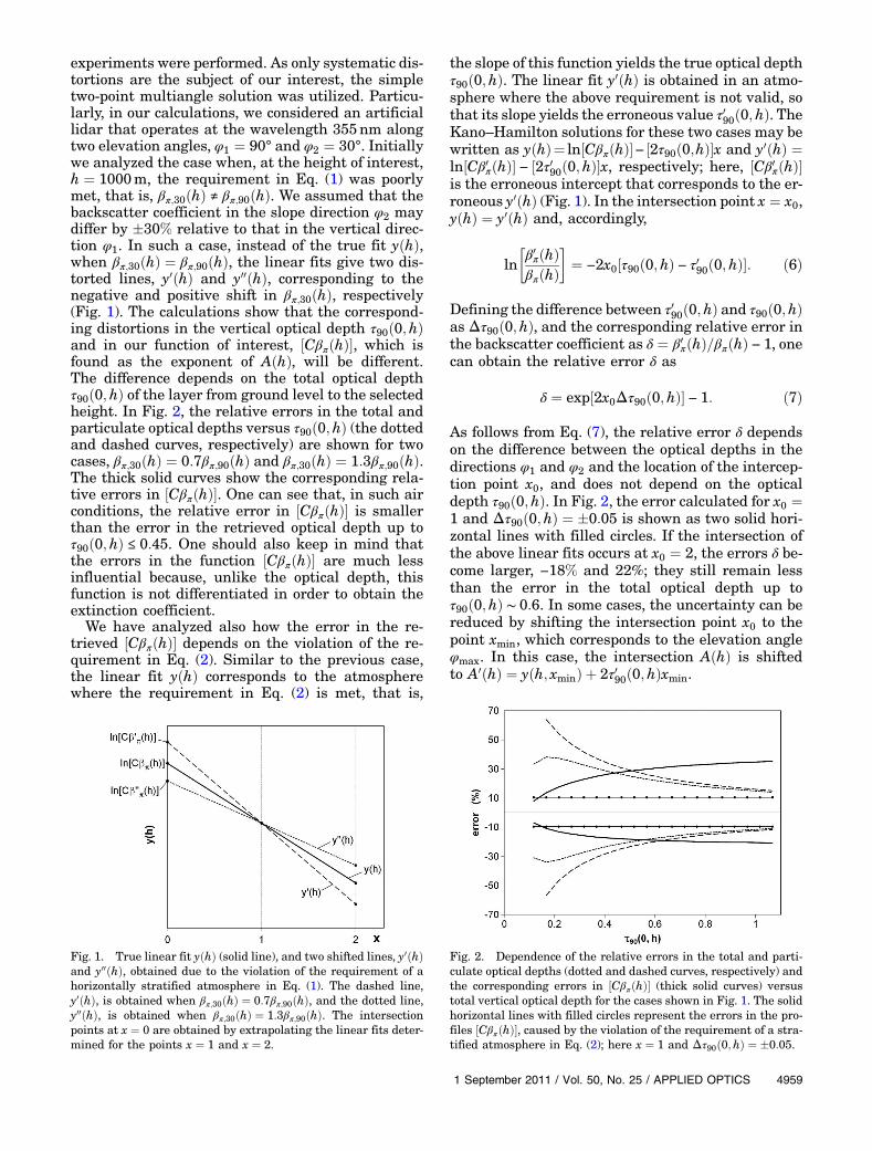
experiments were performed. As only systematic dis-tortions are the subject of our interest, the simpletwo-point multiangle solution was utilized. Particu-larly, in our calculations, we considered an artificiallidar that operates at the wavelength 355nm alongtwo elevation angles, φ1 ¼ 90° and φ2 ¼ 30°. Initiallywe analyzed the case when, at the height of interest,h ¼ 1000m, the requirement in Eq. (1) was poorlymet, that is, βπ;30ðhÞ ≠ βπ;90ðhÞ. We assumed that thebackscatter coefficient in the slope direction φ2 maydiffer by �30% relative to that in the vertical direc-tion φ1. In such a case, instead of the true fit yðhÞ,when βπ;30ðhÞ ¼ βπ;90ðhÞ, the linear fits give two dis-torted lines, y0ðhÞ and y00ðhÞ, corresponding to thenegative and positive shift in βπ;30ðhÞ, respectively(Fig. 1). The calculations show that the correspond-ing distortions in the vertical optical depth τ90ð0;hÞand in our function of interest, ½CβπðhÞ�, which isfound as the exponent of AðhÞ, will be different.The difference depends on the total optical depthτ90ð0;hÞ of the layer from ground level to the selectedheight. In Fig. 2, the relative errors in the total andparticulate optical depths versus τ90ð0;hÞ (the dottedand dashed curves, respectively) are shown for twocases, βπ;30ðhÞ ¼ 0:7βπ;90ðhÞ and βπ;30ðhÞ ¼ 1:3βπ;90ðhÞ.The thick solid curves show the corresponding rela-tive errors in ½CβπðhÞ�. One can see that, in such airconditions, the relative error in ½CβπðhÞ� is smallerthan the error in the retrieved optical depth up toτ90ð0;hÞ ≤ 0:45. One should also keep in mind thatthe errors in the function ½CβπðhÞ� are much lessinfluential because, unlike the optical depth, thisfunction is not differentiated in order to obtain theextinction coefficient.

We have analyzed also how the error in the re-trieved ½CβπðhÞ� depends on the violation of the re-quirement in Eq. (2). Similar to the previous case,the linear fit yðhÞ corresponds to the atmospherewhere the requirement in Eq. (2) is met, that is,

the slope of this function yields the true optical depthτ90ð0;hÞ. The linear fit y0ðhÞ is obtained in an atmo-sphere where the above requirement is not valid, sothat its slope yields the erroneous value τ090ð0;hÞ. TheKano–Hamilton solutions for these two cases may bewritten as yðhÞ¼ ln½CβπðhÞ�− ½2τ90ð0;hÞ�x and y0ðhÞ ¼ln½Cβ0πðhÞ� − ½2τ090ð0;hÞ�x, respectively; here, ½Cβ0πðhÞ�is the erroneous intercept that corresponds to the er-roneous y0ðhÞ (Fig. 1). In the intersection point x ¼ x0,yðhÞ ¼ y0ðhÞ and, accordingly,

ln�β0πðhÞβπðhÞ

�¼ −2x0½τ90ð0;hÞ − τ090ð0;hÞ�: ð6Þ

Defining the difference between τ090ð0;hÞ and τ90ð0;hÞas Δτ90ð0;hÞ, and the corresponding relative error inthe backscatter coefficient as δ ¼ β0πðhÞ=βπðhÞ − 1, onecan obtain the relative error δ as

δ ¼ exp½2x0Δτ90ð0;hÞ� − 1: ð7Þ

As follows from Eq. (7), the relative error δ dependson the difference between the optical depths in thedirections φ1 and φ2 and the location of the intercep-tion point x0, and does not depend on the opticaldepth τ90ð0;hÞ. In Fig. 2, the error calculated for x0 ¼1 and Δτ90ð0;hÞ ¼ �0:05 is shown as two solid hori-zontal lines with filled circles. If the intersection ofthe above linear fits occurs at x0 ¼ 2, the errors δ be-come larger, −18% and 22%; they still remain lessthan the error in the total optical depth up toτ90ð0;hÞ ∼ 0:6. In some cases, the uncertainty can bereduced by shifting the intersection point x0 to thepoint xmin, which corresponds to the elevation angleφmax. In this case, the intersection AðhÞ is shiftedto A0ðhÞ ¼ yðh; xminÞ þ 2τ090ð0;hÞxmin.

Fig. 1. True linear fit yðhÞ (solid line), and two shifted lines, y0ðhÞand y00ðhÞ, obtained due to the violation of the requirement of ahorizontally stratified atmosphere in Eq. (1). The dashed line,y0ðhÞ, is obtained when βπ;30ðhÞ ¼ 0:7βπ;90ðhÞ, and the dotted line,y00ðhÞ, is obtained when βπ;30ðhÞ ¼ 1:3βπ;90ðhÞ. The intersectionpoints at x ¼ 0 are obtained by extrapolating the linear fits deter-mined for the points x ¼ 1 and x ¼ 2.

Fig. 2. Dependence of the relative errors in the total and parti-culate optical depths (dotted and dashed curves, respectively) andthe corresponding errors in ½CβπðhÞ� (thick solid curves) versustotal vertical optical depth for the cases shown in Fig. 1. The solidhorizontal lines with filled circles represent the errors in the pro-files ½CβπðhÞ�, caused by the violation of the requirement of a stra-tified atmosphere in Eq. (2); here x ¼ 1 and Δτ90ð0;hÞ ¼ �0:05.


B. Extraction of the Slope Transmission Profile from½CβπðhÞ� and the Corresponding Square-Range-CorrectedSignal and Determination of the Extinction Coefficientthrough Numerical Differentiation

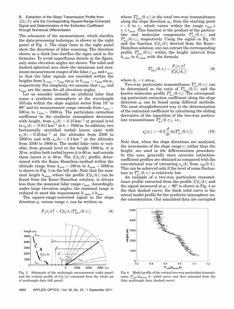
The schematic of the measurement, which clarifiesthe data-processing technique, is shown in the rightpanel of Fig. 3. The slope lines in the right panelshow the directions of lidar scanning. The directionshown as a thick line clarifies the signs used in theformulas. To avoid superfluous details in the figure,only some elevation angles are shown. The solid anddashed spherical arcs show the minimum and max-imummeasurement ranges of the lidar, rmin and rmax,so that the lidar signals are recorded within theheights from hi;min ¼ rmin sinφi to hi;max ¼ rmax sinφi,respectively. For simplicity, we assume that rmin andrmax are the same for all elevation angles.

Let us consider initially an artificial lidar thatscans a synthetic atmosphere at the wavelength355nm within the slope angular sector from 10° to90° and its measurement range extends from rmin ¼500m to rmax ¼ 7000m. The particulate extinctioncoefficient in the synthetic atmosphere decreaseswith height, from κpðhÞ ¼ 0:15km−1 at ground levelto κpðhÞ ¼ 0:011km−1 at h ¼ 7000m. In addition, twohorizontally stratified turbid layers exist withκpðhÞ ¼ 0:25km−1 at the altitudes from 2500 to3000m and with κpðhÞ ¼ 0:1km−1 at the altitudesfrom 3500 to 3800m. The model lidar ratio is vari-able; from ground level to the height 1000m, it is20 sr, within both turbid layers it is 60 sr, and outsidethese layers it is 30 sr. The ½CβπðhÞ� profile, deter-mined with the Kano–Hamilton method within thealtitude range from hmin ¼ 180m to hmax ¼ 5000mis shown in Fig. 3 on the left side. Note that the max-imal height hmax, where the profile ½CβπðhÞ� can befound from the Kano–Hamilton solution, is alwaysless than the maximal lidar range rmax. Accordingly,under large elevation angles, the maximal range isreduced to meet the requirement hi;max ≤ hmax.

The square-range-corrected signal in the slopedirection φi versus range ri can be written as

PiðriÞr2i ¼ CβπðriÞT2tot;ið0; riÞ; ð8Þ

where T2tot;ið0; riÞ is the total two-way transmittance

along the slope direction φi, from the starting pointr ¼ 0 to ri, which varies within the range rmin ≤

ri ≤ rmax. This function is the product of the particu-late and molecular components T2

p;ið0; riÞ andT2

m;ið0; riÞ, respectively. Using the signal in Eq. (8)and the function ½CβπðhÞ� derived from the Kano–Hamilton solution, one can extract the correspondingprofile T2

tot;ið0; riÞ within the height interval fromhi;min to hi;max with the formula

T2tot;ið0; riÞ ¼

PiðriÞr2i½CβπðhiÞ�

; ð9Þ

where hi ¼ ri sinφi.Two-way particulate transmittance T2

p;ið0; riÞ canbe determined as the ratio of T2

tot;ið0; riÞ and theknown molecular profile T2

m;ið0; riÞ. The correspond-ing particulate extinction coefficient along the slopedirection φi can be found using different methods.The most straightforward way is the determinationof the extinction coefficient by calculating the slidingderivative of the logarithm of the two-way particu-late transmittance T2

p;ið0; riÞ, i.e.,

κ�pðriÞ ¼ −0:5ddr

ln½T2p;ið0; riÞ�: ð10Þ

Note that, when the slope directions are analyzed,the increments of the slope range r, rather than theheight, are used in the differentiation procedure.In this case, generally more accurate extinction-coefficient profiles are obtained as compared with theconventional way of extracting κpðhÞ from τ90ð0;hÞ.This can be achieved only if the level of noise fluctua-tion in T2

p;ið0; riÞ is relatively low.An example of a two-way particulate transmit-

tance profile extracted from the profile ½CβπðhÞ� andthe signal measured at φi ¼ 90° is shown in Fig. 4 asthe thin dashed curve; the thick solid curve is theactual model profile for the synthetic atmosphere un-der consideration. Our simulated data are corrupted

Fig. 3. Schematic of the multiangle measurement (right panel)and the vertical profile of ½CβπðhÞ� extracted from the whole setof multiangle data (left panel).

Fig. 4. Model profile of the vertical two-way particulate transmit-tance T2

p;90ðh90;min;hÞ (solid curve) and that extracted from thelidar multiangle data (dashed curve).


with quasi-random noise and, accordingly, the re-trieved profile T2

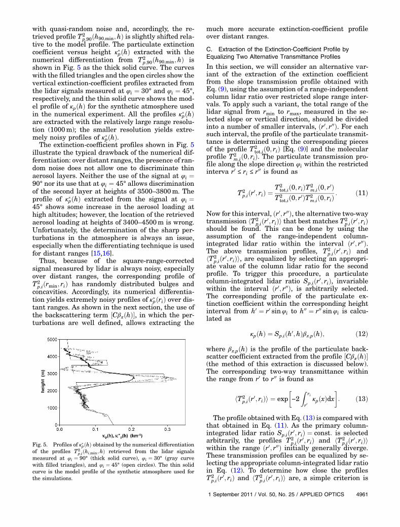
p;90ðh90;min;hÞ is slightly shifted rela-tive to the model profile. The particulate extinctioncoefficient versus height κ�pðhÞ extracted with thenumerical differentiation from T2

p;90ðh90;min;hÞ isshown in Fig. 5 as the thick solid curve. The curveswith the filled triangles and the open circles show thevertical extinction-coefficient profiles extracted fromthe lidar signals measured at φi ¼ 30° and φi ¼ 45°,respectively, and the thin solid curve shows the mod-el profile of κpðhÞ for the synthetic atmosphere usedin the numerical experiment. All the profiles κ�pðhÞare extracted with the relatively large range resolu-tion (1000m); the smaller resolution yields extre-mely noisy profiles of κ�pðhÞ.

The extinction-coefficient profiles shown in Fig. 5illustrate the typical drawback of the numerical dif-ferentiation: over distant ranges, the presence of ran-dom noise does not allow one to discriminate thinaerosol layers. Neither the use of the signal at φi ¼90° nor its use that at φi ¼ 45° allows discriminationof the second layer at heights of 3500–3800m. Theprofile of κ�pðhÞ extracted from the signal at φi ¼45° shows some increase in the aerosol loading athigh altitudes; however, the location of the retrievedaerosol loading at heights of 3400–4500m is wrong.Unfortunately, the determination of the sharp per-turbations in the atmosphere is always an issue,especially when the differentiating technique is usedfor distant ranges [15,16].

Thus, because of the square-range-correctedsignal measured by lidar is always noisy, especiallyover distant ranges, the corresponding profile ofT2

p;iðrmin; riÞ has randomly distributed bulges andconcavities. Accordingly, its numerical differentia-tion yields extremely noisy profiles of κ�pðriÞ over dis-tant ranges. As shown in the next section, the use ofthe backscattering term ½CβπðhÞ�, in which the per-turbations are well defined, allows extracting the

much more accurate extinction-coefficient profileover distant ranges.

C. Extraction of the Extinction-Coefficient Profile byEqualizing Two Alternative Transmittance Profiles

In this section, we will consider an alternative var-iant of the extraction of the extinction coefficientfrom the slope transmission profile obtained withEq. (9), using the assumption of a range-independentcolumn lidar ratio over restricted slope range inter-vals. To apply such a variant, the total range of thelidar signal from rmin to rmax, measured in the se-lected slope or vertical direction, should be dividedinto a number of smaller intervals, ðr0; r00Þ. For eachsuch interval, the profile of the particulate transmit-tance is determined using the corresponding piecesof the profile T2

tot;ið0; riÞ [Eq. (9)] and the molecularprofile T2

m;ið0; riÞ. The particulate transmission pro-file along the slope direction φi within the restrictedinterva r0 ≤ ri ≤ r00 is found as

T2p;iðr0; riÞ ¼

T2tot;ið0; riÞT2

m;ið0; r0ÞT2

tot;ið0; r0ÞT2m;ið0; riÞ

: ð11Þ

Now for this interval, ðr0; r00Þ, the alternative two-waytransmission hT2

p;iðr0; riÞi that best matches T2p;iðr0; riÞ

should be found. This can be done by using theassumption of the range-independent column-integrated lidar ratio within the interval ðr0; r00Þ.The above transmission profiles, T2

p;iðr0; riÞ andhT2

p;iðr0; riÞi, are equalized by selecting an appropri-ate value of the column lidar ratio for the secondprofile. To trigger this procedure, a particulatecolumn-integrated lidar ratio Sp;iðr0; riÞ, invariablewithin the interval ðr0; r00Þ, is arbitrarily selected.The corresponding profile of the particulate ex-tinction coefficient within the corresponding heightinterval from h0 ¼ r0 sinφi to h00 ¼ r00 sinφi is calcu-lated as

κpðhÞ ¼ Sp;iðh0;hÞβπ;pðhÞ; ð12Þ

where βπ;pðhÞ is the profile of the particulate back-scatter coefficient extracted from the profile ½CβπðhÞ�(the method of this extraction is discussed below).The corresponding two-way transmittance withinthe range from r0 to r00 is found as

hT2p;iðr0; riÞi ¼ exp

�−2

Zri

r0κpðxÞdx

�: ð13Þ

The profile obtained with Eq. (13) is compared withthat obtained in Eq. (11). As the primary column-integrated lidar ratio Sp;iðr0; riÞ ¼ const: is selectedarbitrarily, the profiles T2

p;iðr0; riÞ and hT2p;iðr0; riÞi

within the range ðr0; r00Þ initially generally diverge.These transmission profiles can be equalized by se-lecting the appropriate column-integrated lidar ratioin Eq. (12). To determine how close the profilesT2

p;iðr0; riÞ and hT2p;iðr0; riÞi are, a simple criterion is

Fig. 5. Profiles of κ�pðhÞ obtained by the numerical differentiationof the profiles T2

p;iðhi;min;hÞ retrieved from the lidar signalsmeasured at φi ¼ 90° (thick solid curve), φi ¼ 30° (gray curvewith filled triangles), and φi ¼ 45° (open circles). The thin solidcurve is the model profile of the synthetic atmosphere used forthe simulations.


implemented that compares the slopes of the linearfits of these profiles over the selected range ðr0; r00Þ.As both profiles decrease with range, the linear fitsof these can be written in the standard form

T2p;iðr0; riÞ ¼ A1 − B1ri; ð14Þ

hT2p;iðr0; riÞi ¼ A2 − B2ri: ð15Þ

The only task now is to find such a column-integratedlidar ratio Spðr0; riÞ that minimizes the criterion

Λ ¼ ðB1 − B2Þ2: ð16Þ

After the criterionΛ is minimized, the correspondingprofile of κpðhÞ in Eq. (12) is taken as the extinction-coefficient profile of interest over the correspondingaltitude range from h0 to h00. The operations inEqs. (11)–(16) are repeated for all the piecewisezones ðr0; r00Þ selected within the altitude rangeðhi;min;hi;maxÞ. For each such interval, the constantcolumn-integrated lidar ratio is found that mini-mizes the value of Λ in Eq. (16).

The use of the linear fit for the transmission profileT2

p;iðr0; riÞ makes it also possible to elaborate on themaximal measurement range of the lidar signal,rmax. There is a simple requirement, B1 > 0, whichshould be met when selecting the last intervalðr0N ; r00NÞ. If this inequality is not met, the two-waytransmission in this interval will have an unphysicalincrease within this range; the only possibility to sa-tisfy the requirement of the positive B1 is to reducethe maximal range rmax as much as necessary to ob-tain B1 > 0. Note also that the physical minimumB1 ¼ 0means that there is no particulate componentin this range interval (or it is too small to be deter-mined from the measurement data).

The above method of determining the extinctioncoefficient does not require numerical differentiation.However, it requires knowledge of the particulatebackscatter coefficient βπ;pðhÞ in Eq. (12). Obviously,this profile can be determined from the same function½CβπðhÞ� if the constant C is someway estimated. Inthe clear atmospheres for which this method is basi-cally assumed, the constant can be found by using theconventional assumption of pure molecular scatter-ing at high altitudes. If a reference height href is se-lected somewhere close to the maximal height, andthe backscatter coefficient βπ;pðhref Þ ¼ 0, then the con-stant C can be found as

C ¼ ½Cβπðhref Þ�βπ;mðhref Þ

: ð17Þ

Unlike conventionalmethods, the vertical lidar signalis not used here for determining C. This feature canprovide a more accurate determination of the con-stant as compared to that found from the small lidarsignal at the far-end range. As one can see in Fig. 3,

hmax is always less than rmax. Therefore, it is usefuladditionally to estimate the maximal value of C withthe formula

C ≤ min γðhÞ; ð18Þ

where

γðhÞ ¼ ½CβπðhÞ�βπ;mðhÞ

: ð19Þ

The function γðhÞ is determined within the totalheight interval hmin ≤ h ≤ hmax in which ½CβπðhÞ� isknown.AfterC is estimated, the particulate backscat-ter coefficient profile required for Eq. (12) is found as

βπ;pðhÞ ¼½CβπðhÞ�

C− βπ;mðhÞ: ð20Þ

As follows from Eqs. (18)–(20), the selection of theconstantC larger than theminimumof γðhÞwill resultin the zones with negative values of βπ;pðhÞwithin theanalyzed height interval.

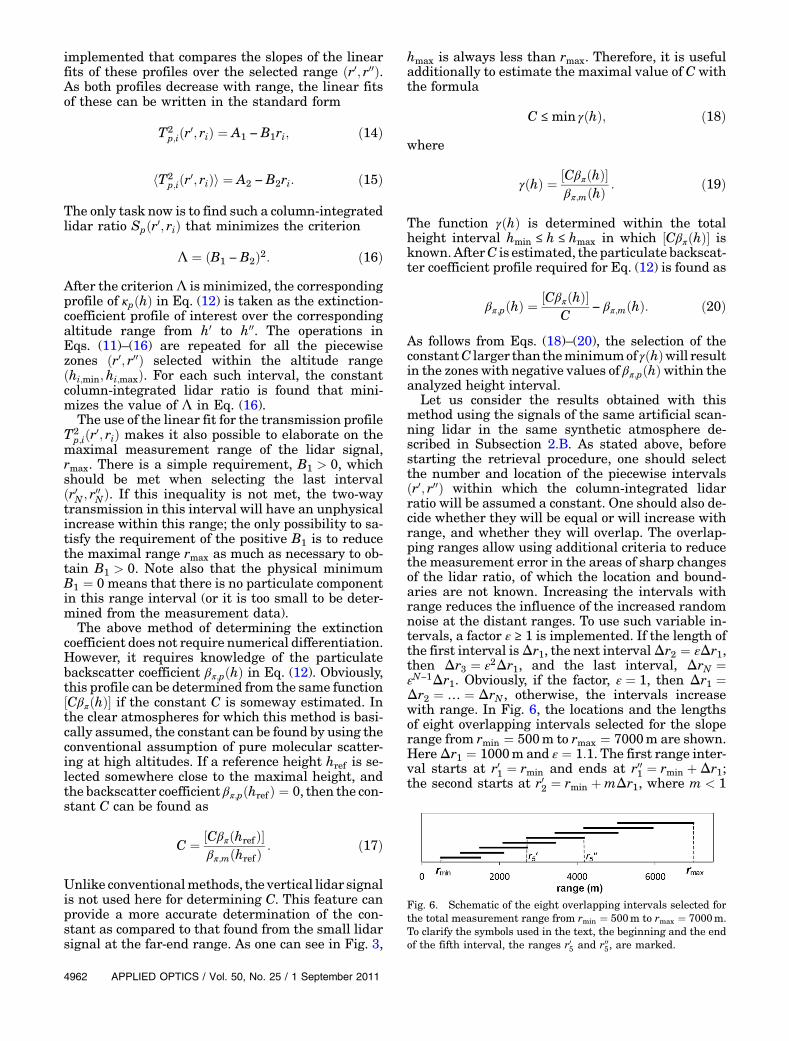
Let us consider the results obtained with thismethod using the signals of the same artificial scan-ning lidar in the same synthetic atmosphere de-scribed in Subsection 2.B. As stated above, beforestarting the retrieval procedure, one should selectthe number and location of the piecewise intervalsðr0; r00Þ within which the column-integrated lidarratio will be assumed a constant. One should also de-cide whether they will be equal or will increase withrange, and whether they will overlap. The overlap-ping ranges allow using additional criteria to reducethe measurement error in the areas of sharp changesof the lidar ratio, of which the location and bound-aries are not known. Increasing the intervals withrange reduces the influence of the increased randomnoise at the distant ranges. To use such variable in-tervals, a factor ε ≥ 1 is implemented. If the length ofthe first interval isΔr1, the next intervalΔr2 ¼ εΔr1,then Δr3 ¼ ε2Δr1, and the last interval, ΔrN ¼εN−1Δr1. Obviously, if the factor, ε ¼ 1, then Δr1 ¼Δr2 ¼ … ¼ ΔrN , otherwise, the intervals increasewith range. In Fig. 6, the locations and the lengthsof eight overlapping intervals selected for the sloperange from rmin ¼ 500m to rmax ¼ 7000m are shown.HereΔr1 ¼ 1000mand ε ¼ 1:1. The first range inter-val starts at r01 ¼ rmin and ends at r001 ¼ rmin þΔr1;the second starts at r02 ¼ rmin þmΔr1, where m < 1

Fig. 6. Schematic of the eight overlapping intervals selected forthe total measurement range from rmin ¼ 500m to rmax ¼ 7000m.To clarify the symbols used in the text, the beginning and the endof the fifth interval, the ranges r05 and r005, are marked.


(in our calculations, the overlapping factor m ¼ 0:5)and ends at r002 ¼ r02 þΔr2. The third interval startsat r03 ¼ r001 and ends at r003 ¼ r03 þΔr3; the fourth inter-val starts at r04 ¼ r002 and ends at r004 ¼ r04 þΔr4, and soon. The last interval starts at r08 ¼ r006 and ends atr008 ¼ rmax. In order not to complicate Fig. 6, onlythe ranges r05 and r005 are marked.

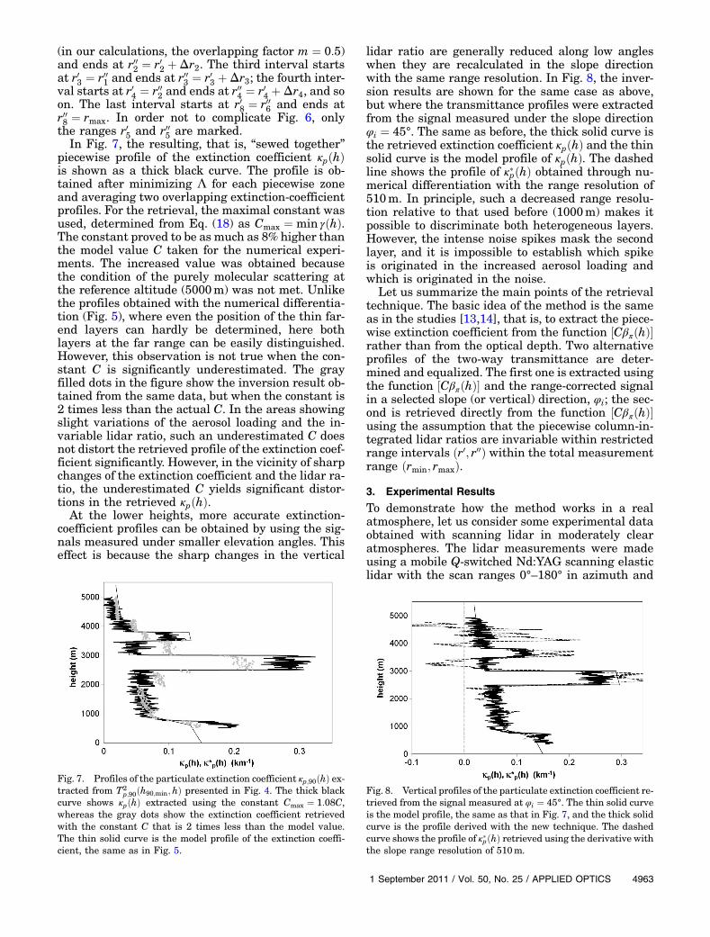
In Fig. 7, the resulting, that is, “sewed together”piecewise profile of the extinction coefficient κpðhÞis shown as a thick black curve. The profile is ob-tained after minimizing Λ for each piecewise zoneand averaging two overlapping extinction-coefficientprofiles. For the retrieval, the maximal constant wasused, determined from Eq. (18) as Cmax ¼ min γðhÞ.The constant proved to be as much as 8% higher thanthe model value C taken for the numerical experi-ments. The increased value was obtained becausethe condition of the purely molecular scattering atthe reference altitude (5000m) was not met. Unlikethe profiles obtained with the numerical differentia-tion (Fig. 5), where even the position of the thin far-end layers can hardly be determined, here bothlayers at the far range can be easily distinguished.However, this observation is not true when the con-stant C is significantly underestimated. The grayfilled dots in the figure show the inversion result ob-tained from the same data, but when the constant is2 times less than the actual C. In the areas showingslight variations of the aerosol loading and the in-variable lidar ratio, such an underestimated C doesnot distort the retrieved profile of the extinction coef-ficient significantly. However, in the vicinity of sharpchanges of the extinction coefficient and the lidar ra-tio, the underestimated C yields significant distor-tions in the retrieved κpðhÞ.

At the lower heights, more accurate extinction-coefficient profiles can be obtained by using the sig-nals measured under smaller elevation angles. Thiseffect is because the sharp changes in the vertical

lidar ratio are generally reduced along low angleswhen they are recalculated in the slope directionwith the same range resolution. In Fig. 8, the inver-sion results are shown for the same case as above,but where the transmittance profiles were extractedfrom the signal measured under the slope directionφi ¼ 45°. The same as before, the thick solid curve isthe retrieved extinction coefficient κpðhÞ and the thinsolid curve is the model profile of κpðhÞ. The dashedline shows the profile of κ�pðhÞ obtained through nu-merical differentiation with the range resolution of510m. In principle, such a decreased range resolu-tion relative to that used before (1000m) makes itpossible to discriminate both heterogeneous layers.However, the intense noise spikes mask the secondlayer, and it is impossible to establish which spikeis originated in the increased aerosol loading andwhich is originated in the noise.

Let us summarize the main points of the retrievaltechnique. The basic idea of the method is the sameas in the studies [13,14], that is, to extract the piece-wise extinction coefficient from the function ½CβπðhÞ�rather than from the optical depth. Two alternativeprofiles of the two-way transmittance are deter-mined and equalized. The first one is extracted usingthe function ½CβπðhÞ� and the range-corrected signalin a selected slope (or vertical) direction, φi; the sec-ond is retrieved directly from the function ½CβπðhÞ�using the assumption that the piecewise column-in-tegrated lidar ratios are invariable within restrictedrange intervals ðr0; r00Þ within the total measurementrange ðrmin; rmaxÞ.3. Experimental Results

To demonstrate how the method works in a realatmosphere, let us consider some experimental dataobtained with scanning lidar in moderately clearatmospheres. The lidar measurements were madeusing a mobile Q-switched Nd:YAG scanning elasticlidar with the scan ranges 0°–180° in azimuth and

Fig. 7. Profiles of the particulate extinction coefficient κp;90ðhÞ ex-tracted from T2

p;90ðh90;min;hÞ presented in Fig. 4. The thick blackcurve shows κpðhÞ extracted using the constant Cmax ¼ 1:08C,whereas the gray dots show the extinction coefficient retrievedwith the constant C that is 2 times less than the model value.The thin solid curve is the model profile of the extinction coeffi-cient, the same as in Fig. 5.

Fig. 8. Vertical profiles of the particulate extinction coefficient re-trieved from the signal measured at φi ¼ 45°. The thin solid curveis the model profile, the same as that in Fig. 7, and the thick solidcurve is the profile derived with the new technique. The dashedcurve shows the profile of κ�pðhÞ retrieved using the derivative withthe slope range resolution of 510m.


0°–90° in elevation. To collect the backscatteredlight, a 25 cm UV enhanced Schmidt–Cassegraintelescope is used. The lidar operated at wavelengthsof 1064 and 355nmwith 98 and 45mJ energy, respec-tively; however, in this study, only data at the wave-length 355nm are used.

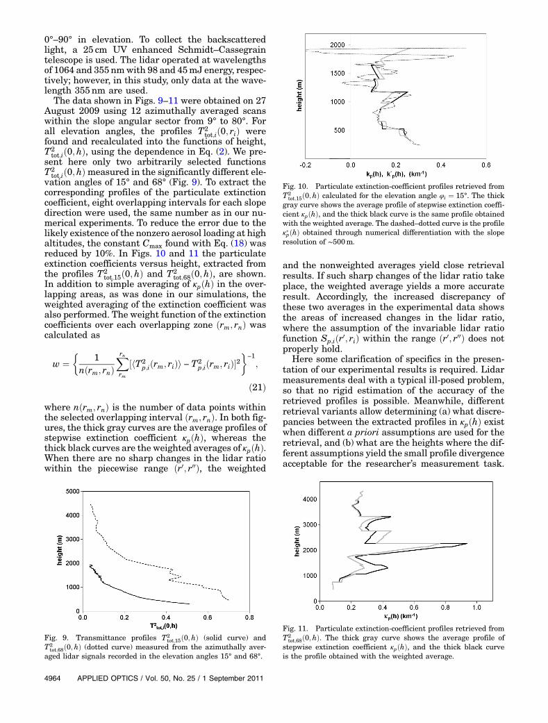
The data shown in Figs. 9–11 were obtained on 27August 2009 using 12 azimuthally averaged scanswithin the slope angular sector from 9° to 80°. Forall elevation angles, the profiles T2

tot;ið0; riÞ werefound and recalculated into the functions of height,T2

tot;ið0;hÞ, using the dependence in Eq. (2). We pre-sent here only two arbitrarily selected functionsT2

tot;ið0;hÞmeasured in the significantly different ele-vation angles of 15° and 68° (Fig. 9). To extract thecorresponding profiles of the particulate extinctioncoefficient, eight overlapping intervals for each slopedirection were used, the same number as in our nu-merical experiments. To reduce the error due to thelikely existence of the nonzero aerosol loading at highaltitudes, the constant Cmax found with Eq. (18) wasreduced by 10%. In Figs. 10 and 11 the particulateextinction coefficients versus height, extracted fromthe profiles T2

tot;15ð0;hÞ and T2tot;68ð0;hÞ, are shown.

In addition to simple averaging of κpðhÞ in the over-lapping areas, as was done in our simulations, theweighted averaging of the extinction coefficient wasalso performed. The weight function of the extinctioncoefficients over each overlapping zone ðrm; rnÞ wascalculated as

w ¼�

1nðrm; rnÞ

Xrnrm

½hT2p;iðrm; riÞi − T2

p;iðrm; riÞ�2�

−1;

ð21Þwhere nðrm; rnÞ is the number of data points withinthe selected overlapping interval ðrm; rnÞ. In both fig-ures, the thick gray curves are the average profiles ofstepwise extinction coefficient κpðhÞ, whereas thethick black curves are the weighted averages of κpðhÞ.When there are no sharp changes in the lidar ratiowithin the piecewise range ðr0; r00Þ, the weighted

and the nonweighted averages yield close retrievalresults. If such sharp changes of the lidar ratio takeplace, the weighted average yields a more accurateresult. Accordingly, the increased discrepancy ofthese two averages in the experimental data showsthe areas of increased changes in the lidar ratio,where the assumption of the invariable lidar ratiofunction Sp;iðr0; riÞ within the range ðr0; r00Þ does notproperly hold.

Here some clarification of specifics in the presen-tation of our experimental results is required. Lidarmeasurements deal with a typical ill-posed problem,so that no rigid estimation of the accuracy of theretrieved profiles is possible. Meanwhile, differentretrieval variants allow determining (a) what discre-pancies between the extracted profiles in κpðhÞ existwhen different a priori assumptions are used for theretrieval, and (b) what are the heights where the dif-ferent assumptions yield the small profile divergenceacceptable for the researcher’s measurement task.

Fig. 9. Transmittance profiles T2tot;15ð0;hÞ (solid curve) and

T2tot;68ð0;hÞ (dotted curve) measured from the azimuthally aver-

aged lidar signals recorded in the elevation angles 15° and 68°.

Fig. 10. Particulate extinction-coefficient profiles retrieved fromT2

tot;15ð0;hÞ calculated for the elevation angle φi ¼ 15°. The thickgray curve shows the average profile of stepwise extinction coeffi-cient κpðhÞ, and the thick black curve is the same profile obtainedwith the weighted average. The dashed–dotted curve is the profileκ�pðhÞ obtained through numerical differentiation with the sloperesolution of ∼500m.


tot;68ð0;hÞ. The thick gray curve shows the average profile ofstepwise extinction coefficient κpðhÞ, and the thick black curveis the profile obtained with the weighted average.


The extinction coefficient κ�pðhÞ retrieved with theslope range resolution 500m is also shown in Fig. 10(the dotted curve). This profile, derived through nu-merical differentiation, agrees well with two othersup to the height ∼1200m, and then large erroneousfluctuations take place; however, these fluctuationsare centered close to two other profiles, which, inturn, are close to each other. One can conclude thatthe assumption of the range-independent Sp;iðr0; riÞover the selected piecewise ranges has been metand the extracted profiles of the extinction coefficientcan be trusted.

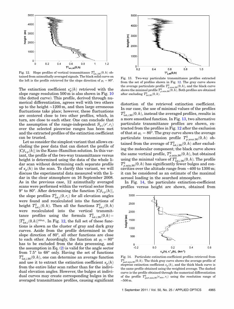
Let us consider the simplest variant that allows ex-cluding the poor data that can distort the profile of½Cβπ;pðhÞ� in the Kano–Hamilton solution. In this var-iant, the profile of the two-way transmittance versusheight is determined using the data of the whole li-dar scan without determining each separate profileof κpðhÞ in the scan. To clarify this variant, we willdiscuss the experimental data measured with the li-dar in the clear atmosphere on 16 September 2008.As in the previous case, 12 azimuthally averagedscans were performed within the vertical sector from9° to 80°. After determining the function ½Cβπ;pðhÞ�,the slope profiles T2

tot;ið0; riÞ for all elevation angleswere found and recalculated into the functions ofheight T2

tot;ið0;hÞ. Then all the functions T2tot;ið0;hÞ

were recalculated into the vertical transmit-tance profiles using the formula T2

tot;i;90ð0;hÞ¼½T2

tot;ið0;hÞ�sinφi . In Fig. 12, the full set of these func-tions is shown as the cluster of gray and dark graycurves. Aside from the profile determined in theslope direction of 80°, all other functions are closeto each other. Accordingly, the function at φi ¼ 80°has to be excluded from the data processing, andthe assumption in Eq. (2) is valid for the angle sectorfrom 7:5° to 68° only. Having the set of functionsT2

tot;i;90ð0;hÞ, one can determine an average functionand use it to extract the extinction coefficient κpðhÞfrom the entire lidar scan rather than for the indivi-dual elevation angles. However, the bulges at indivi-dual curves may create corresponding bulges in theaveraged transmittance profiles, causing significant

distortion of the retrieved extinction coefficient.In our case, the use of minimal values of the profilesT2

tot;i;90ð0;hÞ, instead the averaged profiles, results ina more smoothed function. In Fig. 13, two alternativeparticulate transmittance profiles are shown, ex-tracted from the profiles in Fig. 12 after the exclusionof that at φi ¼ 80°. The gray curve shows the averageparticulate transmission profile T2

p;aver;90ð0;hÞ ob-tained from the average of T2

tot;i;90ð0;hÞ after exclud-ing the molecular component; the black curve showsthe same vertical profile, T2

p;min;90ð0;hÞ, but obtainedusing the minimal values of T2

tot;i;90ð0;hÞ. The profileT2

p;min;90ð0;hÞ has significantly fewer bulges and con-cavities over the altitude range from ∼400 to 1300m;it can be considered as an estimate of the maximalaerosol loading in the searched atmosphere.

In Fig. 14, the particulate extinction-coefficientprofiles versus height are shown, obtained from

Fig. 12. Slope profiles of vertical transmittance T2tot;i;90ð0;hÞ ob-

tained from azimuthally averaged signals. The black solid curve onthe left is the profile retrieved for the slope direction of φi ¼ 80°.

Fig. 13. Two-way particulate transmittance profiles extractedfrom the set of profiles shown in Fig. 12. The gray curve showsthe average particulate profile T2

p;aver;90ð0;hÞ, and the black curveshows theminimal profileT2

p;min;90ð0;hÞ. Both profiles are obtainedafter excluding T2

tot;80ð0;hÞ.


part;min;90ð0;hÞ. The thick gray curve shows the average profile ofstepwise extinction coefficient κpðhÞ, and the thick black curve isthe same profile obtained using the weighted average. The dashedcurve is the profile obtained through the numerical differentiationof the profile T2

part;min;90ðrmin; riÞ using the resolution range of∼500m.


T2p;min;90ð0;hÞ in Fig. 13. As in the previous example,

before determining βπ;pðhÞ, the constant Cmax wasdecreased by 10%. Similar to Figs. 10 and 11, thethick gray curve shows the average profile of thestepwise extinction coefficient κpðhÞ, and the thickblack curve is the weighted average of κpðhÞ. Thedashed curve shows the profile κ�pðhÞ extractedthrough numerical differentiation; here, the heightresolution 500mwas used. In these results, differentretrieval methods yield relatively similar results.The discrepancy in these curves slightly increasesin the heterogeneous area and at the far end, wherethe numerical differentiation yields minor erroneousnegative values of the extinction coefficient.

4. Summary

In this study, a modified data-processing techniquefor multiangle measurements in clear and moder-ately polluted atmospheres is discussed. The keysubject of interest, the extinction-coefficient profile,is extracted from the backscatter term of the Kano–Hamilton solution and the lidar signal measured un-der the selected elevation angle. For the selecteddirection, the local stepwise column-integrated lidarratios over restricted ranges are found from whichthe piecewise extinction coefficient is derived.Such an approach allows extracting the extinction-coefficient profile both along individual elevationangles and in the vertical direction.

The method allows one to analyze the signals mea-sured in different slope directions and reject the sig-nals that do not obey the condition of atmospherichomogeneity or have significant systematic distor-tions. Using this technique, one can determine,(i) whether the requirements in Eqs. (1) and (2) aresatisfactorily met, (ii) the elevation angles in whichthese conditions are not valid, (iii) whether theindividual signals are significantly corrupted, and(iv) how significant are the discrepancies betweenthe profiles extracted under different elevation an-gles at different altitudes.

Unlike the differentiation method, the new techni-que enables discrimination of thin stratified layeringwith sharp boundaries at the far-end range. Theapproach used in this study also allowsmore realisticestimation of the distortions of the inversion resultswhen compared to the methods based entirely on sta-tistics, when no systematic instrumental errors aretaken into consideration.

This method was used to process the experimentaldata obtained with the Fire Sciences Laboratorylidar both in clear-air conditions and in the vicinityof wildfires, and has demonstrated its value forfuture applications.

References

1. M. Kano, “On the determination of backscattering and extinc-tion coefficient of the atmosphere by using a laser radar,”Papers Meteorol. Geophys. 19, 121–129 (1968).

2. P. M. Hamilton, “Lidar measurement of backscatter andattenuation of atmospheric aerosol,” Atmos. Environ. 3,221–223 (1969).

3. V. A. Kovalev and W. E. Eichinger, Elastic Lidar. Theory,Practice, and Analysis Methods (Wiley-Interscience, 2004),pp. 295–304.

4. D. N. Whiteman, “Application of statistical methods to the de-termination of slope in lidar data,” Appl. Opt. 38, 3360–3369(1999).

5. S. N. Volkov, B. V. Kaul, and D. I. Shelefontuk, “Optimal meth-od of linear regression in laser remote sensing,” Appl. Opt. 41,5078–5083 (2002).

6. F. Rocadenbosch, A. Comeron, and D. Pineda, “Assessment oflidar inversion errors for homogeneous atmospheres,” Appl.Opt. 37, 2199–2206 (1998).

7. L. Fiorani, B. Calpini, L. Jaquet, H. Van den Bergh, andE. Durieux, “Correction scheme for experimental biases in dif-ferential absorption lidar tropospheric ozone measurementsbased on the analysis of shot per shot data samples,” Appl.Opt. 36, 6857–6863 (1997).

8. M. Adam, V. Kovalev, C. Wold, J. Newton, M. Pahlow,W. M. Hao, and M. B. Parlange, “Application of the Kano-Hamilton multiangle inversion method in clear atmospheres,”J. Atmos. Ocean. Technol. 24, 2014–2028 (2007).

9. G. J. Kunz and G. de Leeuw, “Inversion of lidar signalswith the slope method,” Appl. Opt. 32, 3249–3256 (1993).

10. V. Shcherbakov, “Regularized algorithm for Raman lidar dataprocessing,” Appl. Opt. 46, 4879–4889 (2007).

11. B. Cadet, V. Giraud, M. Haeffelin, P. Keckhut, A. Rechou, andS. Baldy, “Improved retrievals of the optical properties of cir-rus clouds by a combination of lidar methods,” Appl. Opt. 44,1726–1734 (2005).

12. V. Kovalev, “Determination of slope in lidar data using aduplicate of the inverted function,” Appl. Opt. 45, 8781–8789(2006).

13. V. A. Kovalev, W. M. Hao, and C. Wold, “Determination of theparticulate extinction-coefficient profile and the column-integrated lidar ratios using the backscatter-coefficient andoptical-depth profiles,” Appl. Opt. 46, 8627–8634 (2007).

14. V. Kovalev, C. Wold, W. M. Hao, and B. Nordgren, “Improvedmethodology for the retrieval of the particulate extinctioncoefficient and lidar ratio from the lidar multiangle measure-ment,” Proc. SPIE 6750, 67501B (2007).

15. G. Pappalardo, A. Amodeo, M. Pandolfi, U. Wandinger,A. Ansmann, J. Bösenberg, V. Matthias, V. Amiridis,F. De Tomasi, M. Frioud, M. Iarioti, L. Komguem,A. Papayannis, F. Rocadenbosch, and X. Wang, “Aerosol lidarintercomparison in the framework of the EARLINET project.3. Raman lidar algorithm for aerosol extinction, backscatter,and lidar ratio,” Appl. Opt. 43, 5370–5385 (2004).

16. S. Godin, A. Carswell, D. Donovan, H. Claude, W. Steinbrecht,I. McDermid, T. McGee, M. Gross, H. Nakane, D. Swart,H. Bergwerff, O. Uchino, P. Gathen, and R. Neuber, “Ozonedifferential absorption lidar algorithm intercomparison,”Appl. Opt. 38, 6225–6236 (1999).


Documents

Modified technique for processing multiangle lidar data measured in clear and moderately polluted atmospheres