Embed Size (px)
Citation preview

HAL Id: pastel-00709055https://pastel.archives-ouvertes.fr/pastel-00709055
Submitted on 17 Jun 2012
HAL is a multi-disciplinary open accessarchive for the deposit and dissemination of sci-entific research documents, whether they are pub-lished or not. The documents may come fromteaching and research institutions in France orabroad, or from public or private research centers.
L’archive ouverte pluridisciplinaire HAL, estdestinée au dépôt et à la diffusion de documentsscientifiques de niveau recherche, publiés ou non,émanant des établissements d’enseignement et derecherche français ou étrangers, des laboratoirespublics ou privés.
Multiphysics modelling and numerical simulation ofGTA weld pools
Abderrazak Traidia
To cite this version:Abderrazak Traidia. Multiphysics modelling and numerical simulation of GTA weld pools. Plasmas.Ecole Polytechnique X, 2011. English. <pastel-00709055>

THESIS
presented to
Ecole Polytechnique
in fulfilment of the thesis requirement for the degree of
Doctor of Ecole Polytechnique
major
Mechanical Engineering
Multiphysics modelling and numerical
simulation of GTA weld pools
defended by
Abderrazak TRAIDIA
on September 14th, 2011
Jury members :
Pr. K. DangVan Ecole Polytechnique ParisTech, France President
Pr. IM. Richardson Delft University of Technology, The Netherlands Reviewer
Pr. M. Bellet Ecole des Mines ParisTech, France Reviewer
Dr. M. Carin University Bretagne Sud, France Examinator
Mr. P. Gilles AREVA NP, France Examinator
Pr. Q.S. Nguyen Ecole Polytechnique ParisTech, France Supervisor
Dr. F. Roger ENSTA ParisTech, France Co-supervisor
CIFRE thesis ENSTA ParisTech - AREVA NP


To my parents, Embarka and Abdenacer
To my wife Nawal and my kids Ismael and Ishaq
To all my professors


Contents
Contents i
acknowledgements 1
Motivations and objectives of the present work 3
1 Introduction to Gas Tungsten Arc Welding Process 7
1.1 Gas Tungsten Arc Welding . . . . . . . . . . . . . . . . . . . . . . . . . . . . . . 8
1.1.1 The process . . . . . . . . . . . . . . . . . . . . . . . . . . . . . . . . . . . 8
1.1.2 Welding parameters . . . . . . . . . . . . . . . . . . . . . . . . . . . . . . 9
1.2 Analysis of the different regions of the process . . . . . . . . . . . . . . . . . . . . 11
1.2.1 The arc plasma . . . . . . . . . . . . . . . . . . . . . . . . . . . . . . . . . 11
1.2.2 The weld pool . . . . . . . . . . . . . . . . . . . . . . . . . . . . . . . . . 13
1.2.3 The solid area . . . . . . . . . . . . . . . . . . . . . . . . . . . . . . . . . 20
1.3 Numerical simulation of GTAW: different approaches . . . . . . . . . . . . . . . . 21
1.3.1 A highly coupled multiphysics problem . . . . . . . . . . . . . . . . . . . . 21
1.3.2 HFF approach . . . . . . . . . . . . . . . . . . . . . . . . . . . . . . . . . 22
1.3.3 TMM approach . . . . . . . . . . . . . . . . . . . . . . . . . . . . . . . . . 26
I Study of spot Gas Tungsten Arc Welding: a 2D modelling 27
2 Study of the weld pool dynamics in pulsed current welding 29
2.1 Mathematical formulation and governing equations . . . . . . . . . . . . . . . . . 31
2.1.1 Heat transfer and fluid flow . . . . . . . . . . . . . . . . . . . . . . . . . . 32
2.1.2 Electromagnetic force field . . . . . . . . . . . . . . . . . . . . . . . . . . . 34
2.1.3 The free surface deformation . . . . . . . . . . . . . . . . . . . . . . . . . 35
2.1.4 The liquid/solid interface . . . . . . . . . . . . . . . . . . . . . . . . . . . 38
2.1.5 Summary of equations . . . . . . . . . . . . . . . . . . . . . . . . . . . . . 39
2.1.6 Geometry and boundary conditions . . . . . . . . . . . . . . . . . . . . . . 40
2.2 Results and discussion . . . . . . . . . . . . . . . . . . . . . . . . . . . . . . . . . 42
2.2.1 Analysis of the weld pool behaviour . . . . . . . . . . . . . . . . . . . . . 43
2.2.2 Effect of operating parameters on the weld pool dynamics . . . . . . . . . 50
PhD Thesis: ”Multiphysics modelling and numerical simulation of GTA weld pools” - Abderrazak Traidia - 2011
i

Contents
2.2.3 Effect of the free surface deformation . . . . . . . . . . . . . . . . . . . . . 58
2.3 Investigating the asymmetry sources in horizontal-position welding: a 2D model . 62
2.3.1 approach . . . . . . . . . . . . . . . . . . . . . . . . . . . . . . . . . . . . 62
2.3.2 Results . . . . . . . . . . . . . . . . . . . . . . . . . . . . . . . . . . . . . 63
2.4 Conclusion of the chapter and limits . . . . . . . . . . . . . . . . . . . . . . . . . 66
3 Numerical and experimental study of arc and weld pool couplings 69
3.1 Development of the mathematical model . . . . . . . . . . . . . . . . . . . . . . . 72
3.1.1 Toward a unified formulation . . . . . . . . . . . . . . . . . . . . . . . . . 73
3.1.2 The electrical conductivity near the electrodes . . . . . . . . . . . . . . . 76
3.1.3 The heat transfer at the arc-electrodes interfaces . . . . . . . . . . . . . . 79
3.1.4 Accounting for the gas flow rate . . . . . . . . . . . . . . . . . . . . . . . 81
3.1.5 Summary of governing equations . . . . . . . . . . . . . . . . . . . . . . . 82
3.1.6 Transport properties of constitutive materials . . . . . . . . . . . . . . . . 82
3.2 Comparison of the results with literature . . . . . . . . . . . . . . . . . . . . . . . 86
3.2.1 Comparison with Hsu study . . . . . . . . . . . . . . . . . . . . . . . . . . 86
3.2.2 Comparison with Tanaka calculations . . . . . . . . . . . . . . . . . . . . 90
3.3 Application I: study of pulsed current GTA welding . . . . . . . . . . . . . . . . 94
3.3.1 Computational domain and boundary conditions . . . . . . . . . . . . . . 94
3.3.2 Results . . . . . . . . . . . . . . . . . . . . . . . . . . . . . . . . . . . . . 97
3.3.3 Experimental validation . . . . . . . . . . . . . . . . . . . . . . . . . . . . 105
3.4 Application II: influence of the shielding gas composition . . . . . . . . . . . . . . 107
3.4.1 Different methods of gas supplying . . . . . . . . . . . . . . . . . . . . . . 107
3.4.2 Analysis of the conventional method . . . . . . . . . . . . . . . . . . . . . 112
3.4.3 Analysis of the alternate method . . . . . . . . . . . . . . . . . . . . . . . 121
3.5 Conclusion of the chapter and limits . . . . . . . . . . . . . . . . . . . . . . . . . 124
II Study of moving Gas Tungsten Arc Welding: A 3D modelling 127
4 Heat transfer and fluid flow in moving GTA welding: a hybrid 2D-3D model 129
4.1 Experimental study . . . . . . . . . . . . . . . . . . . . . . . . . . . . . . . . . . . 132
4.1.1 Experimental set-up . . . . . . . . . . . . . . . . . . . . . . . . . . . . . . 132
4.1.2 Results and discussion . . . . . . . . . . . . . . . . . . . . . . . . . . . . . 134
4.2 A hybrid 2D-3D modelling . . . . . . . . . . . . . . . . . . . . . . . . . . . . . . . 138
4.2.1 The arc-plasma modelling . . . . . . . . . . . . . . . . . . . . . . . . . . . 138
4.2.2 The weld pool modelling . . . . . . . . . . . . . . . . . . . . . . . . . . . . 140
4.2.3 Calculations steps . . . . . . . . . . . . . . . . . . . . . . . . . . . . . . . 147
4.2.4 Materials properties of AISI 316L . . . . . . . . . . . . . . . . . . . . . . . 148
4.3 Numerical Results and discussion . . . . . . . . . . . . . . . . . . . . . . . . . . . 150
4.3.1 2D-computed boundary conditions . . . . . . . . . . . . . . . . . . . . . . 150
4.3.2 Welding without filler metal . . . . . . . . . . . . . . . . . . . . . . . . . . 150
ii
PhD Thesis: ”Multiphysics modelling and numerical simulation of GTA weld pools” - Abderrazak Traidia - 2011

4.3.3 Welding with filler metal . . . . . . . . . . . . . . . . . . . . . . . . . . . 157
4.4 Conclusion of chapter and limits . . . . . . . . . . . . . . . . . . . . . . . . . . . 163
5 Application to horizontal GTA welding 165
5.1 Experimental study . . . . . . . . . . . . . . . . . . . . . . . . . . . . . . . . . . . 167
5.1.1 Experimental set-up . . . . . . . . . . . . . . . . . . . . . . . . . . . . . . 167
5.1.2 Results and discussion . . . . . . . . . . . . . . . . . . . . . . . . . . . . . 168
5.2 Numerical simulation . . . . . . . . . . . . . . . . . . . . . . . . . . . . . . . . . . 170
5.2.1 Accounting for the gravity effects . . . . . . . . . . . . . . . . . . . . . . . 170
5.2.2 Geometry and boundary conditions . . . . . . . . . . . . . . . . . . . . . . 172
5.2.3 Numerical results . . . . . . . . . . . . . . . . . . . . . . . . . . . . . . . . 173
5.2.4 Comparison with experiments . . . . . . . . . . . . . . . . . . . . . . . . . 177
5.3 Application to NGH-GTAW . . . . . . . . . . . . . . . . . . . . . . . . . . . . . . 179
5.3.1 Computational domain and boundary conditions . . . . . . . . . . . . . . 179
5.3.2 Numerical results . . . . . . . . . . . . . . . . . . . . . . . . . . . . . . . . 181
5.3.3 Extension to dissimilar sulfur contents welds . . . . . . . . . . . . . . . . 183
5.4 Conclusion . . . . . . . . . . . . . . . . . . . . . . . . . . . . . . . . . . . . . . . 187
Conclusions and future work 189
Bibliography 195
Appendix A:
Reynolds number during welding 203
Appendix B:
A brief review of the ALE method 205
Appendix C:
General form of the free surface deformation model 207
Nomenclature 211
PhD Thesis: ”Multiphysics modelling and numerical simulation of GTA weld pools” - Abderrazak Traidia - 2011
iii


acknowledgements
This thesis arose in part out of three years of research that has been done since I came to the
Materials and Structures group. During this period I have been supported by a great number of
kind people who contributed to the achievement of the present work. It is a pleasure to convey
my gratitude to them all in my humble acknowledgement.
In the first part I would like to record my gratitude to my supervisor Frederic Roger who
brought me to the extraordinary field of welding simulation. Above all the most needed, he
provided me unflinching encouragement and support in various ways. His truly scientist intuition
and enthusiasm has made him as a constant oasis of ideas and passions in welding research,
which inspire and enrich my growth as a PhD student.
I gratefully acknowledge Prof. Quoc-Son Nguyen for his advice and supervision. Thank you
very much Professor for trusting me.
Many thanks go to Ziad Moumni and Antoine Chaigne who enrolled me as a PhD student in
their laboratory. I am grateful to their contribution in the success of the present research and
hope the welding activity to be a major part of the laboratory research fields.
It is a pleasure to pay tribute to Evelyne Guyot who is at the origin of the thesis subject.
Thank you very much for funding the present work. I gratefully thank Jeanne Schroeder, Thorsten
Marlaud, Francois Thumerel, Claude Guyon and all the members of the Technical Centre at
AREVA NP for their enthusiasm and their great contributions in validating experimentally the
numerical results. I gratefully acknowledge Philippe Gilles for his advice and encouragements.
His experience as a welding expert helped me a lot. Thank you very much for examining the
present work.
I am very grateful to Prof. Ian M Richardson and Prof. Michel Bellet for their constructive
comments. I am thankful that in the midst of their activity, they accepted to be members of the
reading committee.
Many thanks go to Muriel Carin who accepted to be member of the thesis examiners. She
is undoubtedly responsible for the success of this thesis, through the examples shared on the
PhD Thesis: ”Multiphysics modelling and numerical simulation of GTA weld pools” - Abderrazak Traidia - 2011
1
acknowledgements
Comsol Multiphysics website. Thank you very much for your help, your encouragements, your
enthusiasm and the fruitful discussions we got.
A special thank go to Michel Brochard, Emilie Le Guen, Hamide Makhlouf and Changxin
Zhao for their excellent contributions in the trends of welding research. Their thesis manuscripts
gave me clear ideas when needed. Thank you again.
To the role model for hard workers in the lab, Lahcene Cherfa, I would like to thank him for
being highly involved in the welding research group. I am proud to record that I had several
opportunities to work with an exceptionally experienced technician like him.
I would like to thank Corrine Rouby, Olivier Doare, Anne-Lise Gloanec, Bertrand Reynier,
Alain Van Herpen, Patrice Riberty and Regine Tanniere for their enthusiasm and their help
during the three past years.
Collective and individual acknowledgements are also owed to my colleagues whose present
somehow perpetually refreshed, helpful, and memorable. Many thanks go in particular to Alex and
clement DC for creating such a great friendship at the office, for their perpetual humour and help-
ful ideas. It is a pleasure to thank Mohammed, Claire and Xue for their enthusiasm and friendship.
Last but not last, I am pleased and full of emotion to thank Said, Salah, Rahma, Rose, Mehdi,
Chouchou, Issou, Yoyo, Jean-Pierre, Samir, Marco, Fredo, Marine and all my friends for their
great support throughout my life.
2
PhD Thesis: ”Multiphysics modelling and numerical simulation of GTA weld pools” - Abderrazak Traidia - 2011

Motivations and objectives of the present
work
The present thesis is funded and done in close collaboration with AREVA NP, Technical Centre.
Industrial need
Currently, arc welding is taking a leading position among other joining processes in the manufac-
turing industry, and more particularly for components requiring high quality assemblies, with
few defects. In the nuclear industry, where high quality is required to guarantee the safety of
power plant installations, welding is used for the assembly of almost all components.
The high thickness of tubular structures in nuclear manufacturing has led welding engineers to
use Narrow-Gap Welding technique. As seen in figure 1, a narrow groove is realised in each pipe,
and an adapted welding torch is used to ensure the integrity of the joining operation. Due to the
high thickness of structures, the welding operation is realised in a multi-pass mode. Moreover, as
the architecture of nuclear power plants is quite complex and components are relatively heavy,
welding operations are often conducted in ’non-flat’ positions; i.e., horizontal, vertical, orbital
and even overhead positions. Additionally, GTAW is used in a pulsed current mode to reduce
distorsions and to guarantee a high level of quality.
The complexity of the previously described welding configuration introduces phenomena that
are not commonly observed during flat-position welding. Figure 1 shows a macrograph of the
weld shape during the assembly of two thick pipes using Narrow-Gap Horizontal-position GTAW
(hereafter called NGH-GTAW). As seen, an asymmetry of lateral penetrations is observed; the
penetration of the weld in the upper pipe is greater than that in the lower one. Moreover, the
free surface of the weld is deformed towards the bottom due to the effect of gravity acting on
the top surface of the weld pool. These phenomena can lead to critical situations, since in some
cases a missed joint at the bottom pipe can even occur (unacceptable in the nuclear industry).
To reduce these phenomena, many experimental tests were conducted, varying the pulse
parameters, the welding speed, the feeding wire characteristics and the welding electrode angle.
This resulted in an improvement of the weld quality. However, the asymmetry in the lateral pen-
etrations of welds was still present. The need for industry to predict the final weld characteristics
and availability of computing facilities and software packages are two reasons to numerically
PhD Thesis: ”Multiphysics modelling and numerical simulation of GTA weld pools” - Abderrazak Traidia - 2011
3

Motivations and objectives of the present work
investigate the effects of welding parameters on GTA weld pool developments.This would make it
possible to point out the factors leading to asymmetrical weld shapes and possibly to numerically
determine the optimum welding parameters to use.
Figure 1: Schematic representation of NGH-GTAW configuration (left). Cross-section macrograph
of a horizontal NGH-GTA stainless steel weld in pulsed heating conditions (right). Courtesy of
the Technical Center AREVA NP.
Objectives and approach
It is obvious that some of the topics of GTAW require years to study. The focus of the present
work is on the mathematical modelling and numerical simulation of the weld pool behaviour
during both stationary and moving torch GTAW. We are also focused on the effects of pulsed
current welding on the weld pool dynamics, which are still misunderstood. The final aim is
to build a three-dimensional weld pool model for GTAW with filler metal, so as to simulate
NGH-GTAW and thus to understand the sources of asymmetries observed experimentally. The
present study will lay a foundation toward the implementation in the near future of optimisation
algorithms that will numerically estimate the optimum welding parameters to use.
The present work is divided into two parts; the first part is devoted to the study of stationary
GTAW, whereas the second part focuses on studying moving GTAW with filler metal.
The first chapter of this work briefly describes the GTA welding process and the physical
phenomena involved, which emphasizes the need for a multiphysics approach for the modelling
of GTAW. It also gives a general state-of-the-art of the numerical simulation of this process and
details the advantages and drawbacks of each approach.
The second chapter deals with the mathematical modelling and numerical simulation of
4
PhD Thesis: ”Multiphysics modelling and numerical simulation of GTA weld pools” - Abderrazak Traidia - 2011

Motivations and objectives of the present work
stationary GTAW. Using a 2D transient weld pool model, we analyse the weld pool dynamics
and the resultant weld shapes during both constant and pulsed current welding. This makes it
possible to numerically investigate the impact of welding parameters on the results, and to give
important conclusions on the choice of these parameters. We also quantify the impact of the
free surface deformation on the weld shape, and point out whether a two-way couplings with the
weld pool calculations is necessary.
To improve the model predictivity, we propose in the third chapter a two-dimensional coupled
arc/weld-pool model, accounting for the electrode, the arc plasma and the workpiece domains.
This makes it possible to get the boundary conditions at the workpiece surface without any
assumption on their radial distributions. It also makes it possible to study the influence of the
chemical composition of the shielding gas, and some new welding techniques such as GTAW with
alternate supply of shielding gases. The computed results are first compared with some studies
available in the literature, then validated from weld macrographs and on a real-time visualisation
of the weld pool development using an infrared camera.
The fourth chapter is devoted to an experimental and numerical study of moving GTA weld
pools with filler metal. To avoid the use of arbitrary Gaussian distributions for the heat fluxes
and current densities, a hybrid 2D-3D approach is presented; the boundary conditions at the
workpiece surface are computed in 2D, whereas the steady-state weld pool is predicted using
a 3D model. The influence of the feeding wire on the energy balance inside the weld pool is
included. The numerical model is first used for the simulation of flat-position welding and the
computed results are compared with temperature measurements (thermocouples and infrared) at
the reverse side of the workpiece and to the macrograph cross-sections.
The last chapter extends the previous hybrid model to horizontal-position welding, in partic-
ular, the effect of gravity on both the momentum conservation and the free surface deformation
is included. This allows us to reach our final aim, since the model is used to reveal the weld
asymmetry in NGH-GTAW and to investigate the factors at the origin of this phenomenon. A
brief experimental extension to GTA welding of plates with different concentrations of sulfur is
presented, so as to see qualitatively the influence of sulfur gradients on the magnitude of the
weld asymmetry.
PhD Thesis: ”Multiphysics modelling and numerical simulation of GTA weld pools” - Abderrazak Traidia - 2011
5

Motivations and objectives of the present work
6
PhD Thesis: ”Multiphysics modelling and numerical simulation of GTA weld pools” - Abderrazak Traidia - 2011

Chapter 1
Introduction to Gas Tungsten Arc
Welding Process
This chapter briefly presents GTA welding process and the main
involved physical phenomena. It also gives the state-of-the-art in
the numerical simulation of this process and analyses the
advantages and drawbacks of each approach.
Contents
1.1 Gas Tungsten Arc Welding . . . . . . . . . . . . . . . . . . . . . . . . . . . . . . . 8
1.1.1 The process . . . . . . . . . . . . . . . . . . . . . . . . . . . . . . . . . . . . 8
1.1.2 Welding parameters . . . . . . . . . . . . . . . . . . . . . . . . . . . . . . . 9
1.2 Analysis of the different regions of the process . . . . . . . . . . . . . . . . . . . . 11
1.2.1 The arc plasma . . . . . . . . . . . . . . . . . . . . . . . . . . . . . . . . . . 11
1.2.2 The weld pool . . . . . . . . . . . . . . . . . . . . . . . . . . . . . . . . . . 13
1.2.3 The solid area . . . . . . . . . . . . . . . . . . . . . . . . . . . . . . . . . . 20
1.3 Numerical simulation of GTAW: different approaches . . . . . . . . . . . . . . . . 21
1.3.1 A highly coupled multiphysics problem . . . . . . . . . . . . . . . . . . . . . 21
1.3.2 HFF approach . . . . . . . . . . . . . . . . . . . . . . . . . . . . . . . . . . 22
1.3.3 TMM approach . . . . . . . . . . . . . . . . . . . . . . . . . . . . . . . . . . 26
PhD Thesis: ”Multiphysics modelling and numerical simulation of GTA weld pools” - Abderrazak Traidia - 2011
7

1. Introduction to Gas Tungsten Arc Welding Process
Over the past few years, fusion welding has become one of the most commonly used joining
techniques in manufacturing industry. This technique requires a heat source of sufficient intensity
for the formation of the weld pool to ensure the coalescence of the welded plates. According
to the nature of the heat source, fusion welding can be described as: gas welding, arc welding,
resistance welding or high energy beam welding. The most commonly used welding processes in
the arc welding category are:
• Shielded Metal Arc Welding (SMAW)
• Gas Tungsten Arc Welding (GTAW)
• Gas Metal Arc Welding (GMAW)
• Submerged Arc Welding (SAW)
• Electroslag Welding (ESW)
1.1 Gas Tungsten Arc Welding
1.1.1 The process
Due to its high welding quality, compared to other arc welding processes, Gas Tungsten Arc
Welding (GTAW or GTA welding) also called Tungsten Inert Gas (TIG) is currently taking a
leading position for specialist applications. It is widely used in applications that require high
quality assemblies such as the manufacturing of space vehicles and some nuclear power plant
heavy components. A sketch of this process is shown in figure 1.1. As seen is this figure, the
ionisation of a shielding gas flowing around a nozzle creates an arc plasma between two electrodes:
the anode (+) which represents the workpiece and the cathode (-) which represents the welding
electrode. The shielding gas must be inert to protect the weld pool and the welding electrode
from atmospheric oxidation, and easily ionisable to ensure the formation of the arc plasma.
Usually, pure argon or various mixtures of argon-helium or argon-hydrogen are used for their
inert properties with relative low cost (especially for argon).
The welding electrode is made of tungsten for its thermionic aspect (ability to emit electrons
by thermal heating) and its high melting temperature (around 3700 K). To decrease the electrode
work function (which is the minimum energy required to remove an electron from a solid) and to
increase the melting temperature, thorium oxides (ThO2) are generally added to tungsten. This
is called a thoriated tungsten electrode. However, one must mention that for welding of some
materials such as aluminium alloys, the appearance of oxides layers (such as alumina) at the
top surface significantly decreases the weldability. In such a case, a Direct Current Electrode
Positive mode is used, in which the polarity of the welding electrode is alternatively modified.
This creates a cathodic cleaning effect that will eliminate the oxide layers at the top surface of
the weld pool and ensures a better weldability.
8
PhD Thesis: ”Multiphysics modelling and numerical simulation of GTA weld pools” - Abderrazak Traidia - 2011

1.1. Gas Tungsten Arc Welding
Figure 1.1: Schematic representation of GTAW process [1].
Figure 1.2: Main welding positions and their denominations.
1.1.2 Welding parameters
1.1.2.1 Main input parameters
As with any other welding process, GTA welding parameters are chosen as a function of the
required characteristics (materials, geometry, thickness, etc.), but also related to the welding
position (flat ’1g’, horizontal ’2g’, vertical ’3g’ and overhead ’4g’, as shown in figure 1.2). In
practice, the input parameters to be chosen by the welder are as follows:
• The welding current: Continuous Current mode (CC GTAW) or Pulsed Current mode
(PC GTAW). In the case of CC GTAW, the value of the constant current must be chosen.
Whereas for PC GTAW mode, several values must be chosen: the peak and background
currents, the pulse frequency, and the peak pulse duration (see figure 1.3).
• The arc length (inter-electrodes distance that varies from 1 to 5 mm), or the arc voltage
(usually between 10 V and 15 V).
• The welding electrode (material, diameter and tip-angle), and the gas nozzle (internal
diameter, material).
PhD Thesis: ”Multiphysics modelling and numerical simulation of GTA weld pools” - Abderrazak Traidia - 2011
9

1. Introduction to Gas Tungsten Arc Welding Process
• The shielding gas composition (argon, helium, or mixtures of different gases), and the gas
flow rate (usually from 5 to 30 L.min−1).
• The welding speed (from 8 to 20 cm.min−1).
• In the case of filler metal GTA welding, one most specify the feeding wire material (usually
the same as the base metal), diameter (less than 1 mm), and feeding speed (usually less
than 100 cm.min−1).
1.1.2.2 Pulsed current mode
The literature review shows that the use of GTA welding in pulsed current mode is widespread,
for both semi-automatic and automatic welding equipments [2]. A typical pulsed current signal
used in this mode is shown in figure 1.3. As seen the welding current varies between two constant
values, namely; the peak and background currents, at a given constant frequency. Either the
peak pulse duration or the background duration can be adjusted by the welder.
Pulsing the welding current with time has been experimentally reported to have great
advantages:
• It improves the arc stability in vertical and overhead welding positions [2].
• It produces a deeper and wider weld than that of the corresponding mean current welding
[2].
• It avoids weld cracks and reduces the residual stresses and distortions after cooling [2].
• It produces a finer grain size and smaller martensitic platelates with less tendency to
segregation. This results in a better weld strength and an improved ductility compared to
that for continuous current welds [3].
The above mentioned advantages of PC GTA welding explain its widespread use in the nuclear
manufacturing industry where the high safety of assemblies and the limitations of welding defects
must be guaranteed.
Ip
Ib
tp
tb
1/f
Welding current
Time
Ip: peak current
Ib: background current
tp
: peak pulse duration
tb: background pulse duration
f: pulse frequency
Figure 1.3: A typical pulsed current welding used in PC GTAW mode.
10
PhD Thesis: ”Multiphysics modelling and numerical simulation of GTA weld pools” - Abderrazak Traidia - 2011

1.2. Analysis of the different regions of the process
1.2 Analysis of the different regions of the process
Figure 1.4: Main physical phenomena that occur during GTAW
The main physical phenomena that occur during GTA welding are shown in figure 1.4. It is
shown that four states (solid, liquid, gas and plasma) of several materials exist simultaneously in
a small volume. Then, physical interactions associated with electric, magnetic, thermal, chemical,
solid and fluid processes take place. The whole welding process is generally divided into three
zones: the arc plasma zone, the weld pool zone and the solid zone (HAZ and base metal). These
three zones are described in the next paragraphs.
1.2.1 The arc plasma
An arc plasma can be defined as a discharge of electricity between two electrodes (anode and
cathode) in a gaseous phase, in which (a) the voltage drop at the cathode is in the order of
excitation potential of the electrode (about 10 V) and (b) the current density can have any value
above a minimum of 106 A m−2 [4].
A schematic representation of the electric field distribution along the arc axis is presented
in figure 1.5. By considering this non-uniform evolution, the arc plasma zone can be divided
into three regions: the arc column, the cathode region and the anode region. A brief description
of each region is given below. Readers interested in a more complete description are invited to
consult the recently published review of Richardson [5].
1.2.1.1 The arc column
The arc column which represents most of the volume of the arc plasma consists of neutral particles
(atoms or molecules) and charged particles (ions and electrons). It is assumed that this region is
PhD Thesis: ”Multiphysics modelling and numerical simulation of GTA weld pools” - Abderrazak Traidia - 2011
11

1. Introduction to Gas Tungsten Arc Welding Process
electrically neutral, thus the number of negative and positive species are almost the same.
At high temperatures (above 6000 K), the shielding gas is decomposed into ions and electrons,
which ensures the electrical conductivity of the arc column. Using principles of thermodynamics,
it is possible to calculate the degree of dissociation of the plasma. An example of the calculated
composition of argon plasma as function of temperature is given in figure 1.6. At low temperatures
argon just consists of neutral atoms, whereas at higher temperatures, it first dissociates into
singly, then into doubly and even triply ionised atoms and electrons.
Figure 1.5: Evolution of the electric potential along the arc plasma axis.
Figure 1.6: Calculated composition of an argon plasma as a function of temperature at a pressure
of 1 bar [6].
A very important assumption that is considered inside the arc column is that collisions
12
PhD Thesis: ”Multiphysics modelling and numerical simulation of GTA weld pools” - Abderrazak Traidia - 2011

1.2. Analysis of the different regions of the process
between particles dominates over other physical processes such as applied forces, diffusion or
radiation [6]. This leads to an equidistribution of kinetic energy inside the arc column and
results in what is commonly called the ’Local Thermodynamic Equilibrium’ or ’LTE’. One of the
main consequences of the ’LTE’ assumption is that the average temperatures of each species of
particles inside the arc plasma is equal. This assumption of the arc plasma being in ’LTE’ is
commonly considered, it avoids the development of a twin temperature model (separate ions and
electron temperatures) for the modelling of the arc plasma area. However, one must note that
near the electrodes (cathode and anode) several ’non-LTE’ effects occur leading to a difference
between the ions and electrons temperatures and densities. The main non-LTE effects occur
at the fringes of the arc column, and the numerical techniques used for their modelling will be
detailed later in this manuscript.
1.2.1.2 The anode region
The second part of the arc plasma area is the anode region, which receives the emitted electrons
from the cathode. This relatively thin region acts as an electron-absorbing layer that ensures
the electrical continuity between the arc column and the workpiece. The emitted electrons from
the cathode are accelerated while travelling through the arc column, then they hit the anode
and deliver their kinetic energy to the workpiece as a heating effect. This is called the ’electron
condensation heating’. As a consequence, the workpiece is heated from both the arc plasma and
the electrons arriving at the top surface. These heat transfer phenomena will be discussed in
detail in the following chapters.
1.2.1.3 The cathode region
The influence of the previously discussed anode region on the arc plasma properties has been
reported to be less than the cathode [7]. The cathode region is even the most critical part of the
arc plasma. It can be considered as a space bounded by two parallel planes, one representing
the arc column boundary and emitting ions, and the other representing the cathode surface and
emitting electrons.
The emission of electrons from the welding electrode is governed by basic principles of
thermionic emission. When the cathode is heated to a sufficiently high temperature, electrons
are emitted with a current density Jc given by the following Richardson-Dushman equation:
Jc = ArT2 exp
(− eφekBT
)(1.1)
where Ar is the Richardson’s constant, e the elementary charge, kB is the Boltzmann constant
and φe is the effective work function of the cathode material and is defined as the minimum
energy that must be supplied to an electron to overcome the surface forces.
1.2.2 The weld pool
After the arc plasma, the second important zone to be described is the weld pool. According to
the workpiece material and to the welding energy, a weld pool of few millimetres in dimensions is
PhD Thesis: ”Multiphysics modelling and numerical simulation of GTA weld pools” - Abderrazak Traidia - 2011
13

1. Introduction to Gas Tungsten Arc Welding Process
created by the heating from the arc plasma. It is well reported in the literature [8, 9, 10, 11, 12,
13, 14] that both the characteristics of the weld joint (dimensions, shape, microstructure, etc.)
and the heat transfer at the solid/liquid interface are highly dependent on the fluid flow in the
weld pool. As a result, to get a good prediction of the weld shape as well as thermal cycles and
the induced residual stresses around the weld zone (where the risk of fracture is highest), one
must take into account the development of the weld pool and its dynamics with time.
The molten metal flow is governed by the combination of various forces that can be classified
into two categories: the volumetric forces and the surface forces.
1.2.2.1 The volumetric forces
The volumetric forces are the combination of the gravity forces, and the electromagnetic forces.
Gravity forces
At first glance, one might think the gravity force in the weld pool is only made of the classical
inertia force ~Fi = ρ0~g. However, the high thermal gradients that take place in the weld pool
induce a natural convection flow (buoyancy effect) due to the dependence of molten metal density
on temperature. This buoyancy effect can be modelled by an additional force ~Fb using the
Boussinesq approximation as follows [12]:
−→Fb = −ρ0β(T − Tref )−→g (1.2)
where ρ0, β and Tref are respectively reference density, thermal expansion and a reference
temperature of the molten pool. It should be noted that in most of the available weld pool
models, the inertia force is neglected, and therefore the gravity force is only made of the buoyancy
force. Even though, the gravity force is approximately 10 times larger than the buoyancy force,
it does not contribute to the creation of flows, since contrary to buoyancy force, it is constant
and does not present any spatial gradient in the weld pool. However, it has a significant impact
on the free surface shape, as detailed further.
As shown in figure 1.7, buoyancy forces tend to create outward flow which increases the weld
pool width. Concerning the relative importance of this force toward the other governing forces,
Tanaka et al.[15] reported that the velocity field induced by only the buoyancy effect is 10 times
lower than that induced by surface forces (combination of the Marangoni shear stress and the
arc drag force). However, it should be mentioned that the conclusions of Tanaka et al.[15] are for
the flat welding position. Up to the present, far less work has been conducted to study the effect
of buoyancy force on the weld shape for horizontal, vertical or overhead welding positions. This
point will be studied in the following chapters.
14
PhD Thesis: ”Multiphysics modelling and numerical simulation of GTA weld pools” - Abderrazak Traidia - 2011

1.2. Analysis of the different regions of the process
Figure 1.7: 2D axisymmetric representation of the molten metal flow directions induced by the
main driving forces in the weld pool.
Electromagnetic forces
The electromagnetic forces also called Lorentz forces are the combination of the current flow and
the induced magnetic field in the weld pool. For a stationary welding electrode, as the positive
current flows from the workpiece to the cathode, the main component of the current density
vector−→j is ascendant along the arc axis (+−→ez ), therefore, the magnetic field vector
−→B is in the
positive azimuthal direction (+−→eθ ). This results in a Lorentz force (−→j ×−→B ) directed toward the
center of the weld pool, which tends to create inward flow and increase the weld pool depth, as
seen in figure 1.7.
Tanaka et al.[16] reported that for pure argon shielding gas, the fluid velocities induced by
only the Lorentz forces are 4 times lower than that induced by surface forces. However, it should
be noted that the chemical composition of the shielding gas has a great impact on the magnitude
of the Lorentz forces, and more particularly when using pure helium gas. This will be discussed
further in the present work.
1.2.2.2 The surface forces
The surface forces acting on the top surface of the molten metal are the sum of the Marangoni
shear stress and the arc drag force.
The arc drag force
The flow of the viscous plasma at the top workpiece surface creates a shear stress directed toward
the edges of the weld pool. This induces an outward flow, which increases the weld pool width
(see figure 1.7). The gas shear stress is reported to be the third main important force in the
weld pool, after the Marangoni shear stress and the Lorentz forces. However, the intensity of
gas shear stress is highly dependent on the welding current and the chemical composition of the
shielding gas. Figure 1.8 shows the computed results of the radial evolution of the gas shear
PhD Thesis: ”Multiphysics modelling and numerical simulation of GTA weld pools” - Abderrazak Traidia - 2011
15

1. Introduction to Gas Tungsten Arc Welding Process
stress for different shielding gases at the same welding current. It is well seen that the arc drag
force is highly dependent on the shielding gas. The maximum value of the shearing stress is even
multiplied by a factor of 2, when adding only 9% of hydrogen to argon.
Figure 1.8: Radial evolution of the arc drag force for different argon-hydrogen mixtures. Welding
current of 200 A with an arc length of 5 mm [17].
The Marangoni shear stress
When high thermal gradients occur at a top surface of a liquid (which is the case during fusion
welding), the surface tension of this liquid becomes non-uniform and liquid particles move from
low to high surface tension regions. This leads to the creation of a flow inside the molten metal:
it is the ’Marangoni effect’, also referred as ’Marangoni driven-flow’, which induces profound
effects on the weld shape [18]. This effect has been identified as the dominant driving force in
GTA weld pools.
Usually, the Marangoni effect at the free surface of the weld pool is described by the following
equation:
µ∇nvs =∂γ
∂T∇sT (1.3)
where µ is dynamic viscosity, T is the pool surface temperature, vs is the tangential velocity,
∇n is the normal gradient operator defined as ∇nX = ∇X · −→n , ∇s is the tangential gradient
operator defined as ∇sX = ∇X−∇nX and −→n and −→s are respectively the normal and tangential
vectors to the free surface of the weld pool.
∂γ
∂Tis commonly called ’the surface tension gradient’ or ’the thermal gradient of surface
tension’. It has been identified that this coefficient has a great influence on the flow directions
in the weld pool [18]. As shown in figure 1.9(a), when this coefficient is negative, the surface
tension is highest at the edges of the weld pool, and then thermocapillary flow is outward from
16
PhD Thesis: ”Multiphysics modelling and numerical simulation of GTA weld pools” - Abderrazak Traidia - 2011

1.2. Analysis of the different regions of the process
low to high surface tension regions which results is a wide and shallow weld. However, when the
surface tension gradient is positive, surface flow is inward and heat is swept to the bottom of the
weld pool and produces a narrow and deep weld.
Figure 1.9: (a) Effect of the surface tension gradient on the fluid flow directions. (b) Effect of
the sulfur content in the welded alloy on the weld shape [6].
This critical coefficient (which depends on temperature) is negative for pure metals, but can
be altered from negative to positive values by the presence of surface-active elements, such as,
sulfur or oxygen. Figure 1.9(b) shows the influence of sulfur content on the final weld shape
during welding of AISI 304 stainless steel. It clearly appears that the addition of sulfur increases
the weld depth due to the change in the sign of∂γ
∂T.
The Sahoo et al. [19] relationship
Although the surface tension phenomenon is well understood, it is quite difficult to quantify.
Sahoo et al. [19] were the first to propose a semi-empirical relationship between the surface
tension gradient, temperature and content of surface-active elements, for various binary alloys.
For binary iron-sulfur systems, the relationship is as follows:
∂γ
∂T= −Aγ −RgΓs ln(1 +Kas)−
Kas1 +Kas
Γs∆H0
T
K(T ) = k1 exp(−∆H0
RgT)
(1.4)
where as is the sulfur content of the workpiece material, Aγ is a constant (usually fixed at
4.3×10⁻⁴ N m−1 K−1), Γs is the surface excess at saturation (1.3×10⁻⁸ kmol m−2), Rg is gas
constant (8314.3 J kmol−1 K−1), k1 is the entropy factor (3.18×10⁻³) and ∆H0 is standard heat
of adsorption, which is estimated from an empirical function of the difference in electronegativity
between the solute and solvent atoms.
PhD Thesis: ”Multiphysics modelling and numerical simulation of GTA weld pools” - Abderrazak Traidia - 2011
17

1. Introduction to Gas Tungsten Arc Welding Process
For a Fe-S binary alloy ∆H0 is estimated to be -1.66×10⁸ J kmol−1. By considering this
value for the heat of adsorption, the evolution of the surface tension gradient with temperature
for various sulfur contents is given in figure 1.10. Analysing this figure shows that for very low
sulfur contents, the surface tension gradient is negative for any temperature, and thus the fluid
flow is outward. Whereas, for very high sulfur contents, the surface tension gradient is positive
in the whole range of temperature, and fluid flow is directed toward the weld axis. However, for
an intermediate sulfur content, a critical temperature Tc exists which corresponds to a change in
the sign of the surface tension gradient, and results in a flow reversal, creating simultaneously
two different vortices.
Figure 1.10: Surface tension gradient as function of temperature and sulfur content for Fe-S
alloys [8] (top), and effect of sulfur content on the reversal flows in the weld pool (bottom).
From the previous considerations, it clearly appears that to get predictive results for the
numerical modelling of the weld pool dynamics, one must consider the Sahoo et al. [19] relationship
for the surface tension gradient. However, the literature review shows that most of the available
models, and more particularly three-dimensional models, assume an arbitrary constant value
of this coefficient in the order of ±10−4 N m−1 K.1. This assumption is usually considered to
reduce computing time, even though the computed results are highly dependent on the chosen
value for∂γ
∂T.
18
PhD Thesis: ”Multiphysics modelling and numerical simulation of GTA weld pools” - Abderrazak Traidia - 2011
1.2. Analysis of the different regions of the process
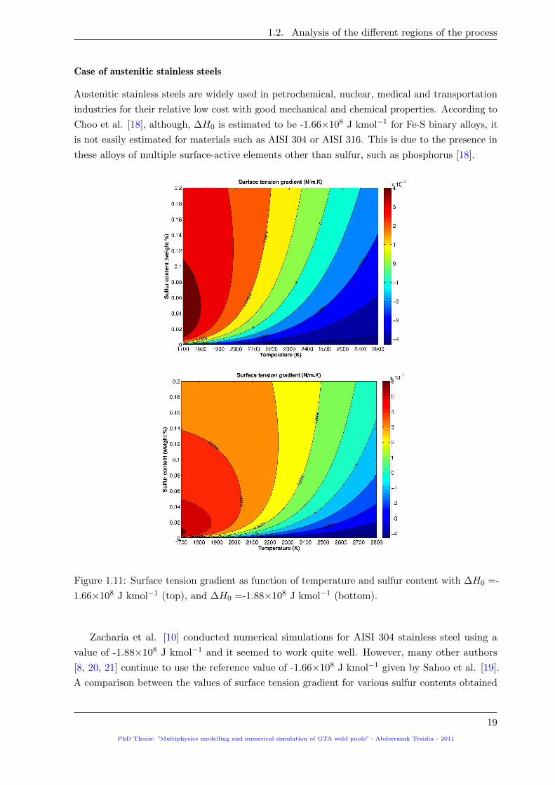
Case of austenitic stainless steels
Austenitic stainless steels are widely used in petrochemical, nuclear, medical and transportation
industries for their relative low cost with good mechanical and chemical properties. According to
Choo et al. [18], although, ∆H0 is estimated to be -1.66×10⁸ J kmol−1 for Fe-S binary alloys, it
is not easily estimated for materials such as AISI 304 or AISI 316. This is due to the presence in
these alloys of multiple surface-active elements other than sulfur, such as phosphorus [18].
Figure 1.11: Surface tension gradient as function of temperature and sulfur content with ∆H0 =-
1.66×10⁸ J kmol−1 (top), and ∆H0 =-1.88×10⁸ J kmol−1 (bottom).
Zacharia et al. [10] conducted numerical simulations for AISI 304 stainless steel using a
value of -1.88×10⁸ J kmol−1 and it seemed to work quite well. However, many other authors
[8, 20, 21] continue to use the reference value of -1.66×10⁸ J kmol−1 given by Sahoo et al. [19].
A comparison between the values of surface tension gradient for various sulfur contents obtained
PhD Thesis: ”Multiphysics modelling and numerical simulation of GTA weld pools” - Abderrazak Traidia - 2011
19

1. Introduction to Gas Tungsten Arc Welding Process
by the two values of ∆H0 is given in figure 1.11. It clearly appears that when considering
∆H0=-1.88×10⁸ J kmol−1 the contour∂γ
∂T= 0 is shifted toward higher values of temperature.
This means that the critical temperature Tc is increased for any value of sulfur content, which
goes in favour of enhancing the region where∂γ
∂T> 0. Besides this fact, ∆H0 which is estimated
from the difference in the electronegativities between the solute and solvent atoms has a certain
uncertainty associated with it, that can be about 10% for Fe-S alloys [18]. Choo et al. [18]
conducted numerical simulations and showed that the sensitivity of the weld pool to ∆H0 is
important. They concluded that a 10% change in ∆H0 can result in large changes in the surface
temperature, velocity profiles and weld shape.
To conclude on the Marangoni effect, it seems to be important to take into account the variation
of the surface tension gradient with temperature and sulfur content, as the thermocapillary flow
affects the circulation in the weld pool, and plays an important role in affecting the weld shape
and the free surface temperature [18]. For AISI 304 stainless steel, it is also important to choose
the right value for the heat of adsorption coefficient ∆H0 to account for the effects of all the
surface-active elements present in the weld pool. In the present work, we will use either the
reference value of Sahoo et al. (-1.66×10⁸ J kmol−1), or the value proposed by Zacharia et al.
(-1.88×10⁸ J kmol−1), depending on the agreement with experiments.
1.2.2.3 Some dimensionless numbers
To quantify the relative importance of the previously described governing forces in the weld pool,
a brief review of the main important dimensionless numbers in welding is given in table 1.1. L is
the characteristic length of the weld pool, ∆T the temperature difference between the maximum
temperature of the weld pool and the solidus temperature, (∂γ/∂T ) the surface tension gradient,
µ the dynamic viscosity, α the thermal diffusivity, ρ the density, µm the magnetic permeability,
I the welding current, and Lb is the characteristic length for the buoyancy in the molten pool.
Table 1.1 clearly shows that the Marangoni shear stress is the predominant governing force in
the weld pool, followed by the electromagnetic forces and the buoyancy convection.
1.2.3 The solid area
The last area of the welding process to be described is the solid region. It corresponds to the
domain of the workpiece that did not reach the melting temperature. It is commonly divided
into two regions: the Heat Affected Zone (HAZ) and the Base Metal (BM).
The HAZ corresponds to the region close to the melted zone that reached so high temperatures
during the welding process that induced metallurgical changes. It also includes the sub-critical
regions where material properties have been altered with respect to the base material (BM),
for example due to carbon diffusion. The HAZ is the main critical region of the weld, where
incompatible plastic strains causing residual stresses are located, and where the risks of fracture
are generally expected.
20
PhD Thesis: ”Multiphysics modelling and numerical simulation of GTA weld pools” - Abderrazak Traidia - 2011

1.3. Numerical simulation of GTAW: different approaches
Number Relationship Description Reported value [22]
MaL∆T (∂γ/∂T )
µαRatio of Marangoni to viscous force 9.4×10⁴
RmρµmI
2
4π2µ2Ratio of Lorentz to viscous force 7×10⁴
Grρ2βL3
b∆T
µ2Ratio of buoyancy to viscous force 30
RS/BMa
GrRatio of Marangoni to buoyancy force 3.1×10³
RM/BRmGr
Ratio of Lorentz to buoyancy force 2.3×10³
Table 1.1: Some classical dimensionless numbers used in GTA welding. Taken from [23]
1.3 Numerical simulation of GTAW: different approaches
1.3.1 A highly coupled multiphysics problem
Fluid flow
Heattransfer
Solidmechanics
Free surfacedeformations
Electromagnetism
Metallurgy
HFF Approach
TMM Approach
Figure 1.12: Multiphysics couplings in arc welding modelling.
By considering the previous study of the different regions that form the GTA welding process, it
appears that the mathematical modelling of such a process involves many phenomena that belong
to different physics: plasma physics, heat transfer, fluid flow, metallurgy, solid mechanics and
PhD Thesis: ”Multiphysics modelling and numerical simulation of GTA weld pools” - Abderrazak Traidia - 2011
21

1. Introduction to Gas Tungsten Arc Welding Process
free surface deformation. Moreover, as shown in figure 1.12, the couplings between the physics
can be either bi-directional (strong couplings), or uni-directional (weak couplings).
A literature review of GTA welding models shows that according to what we are looking for
(prediction of the weld shape, prediction of the residual stresses or study of the arc/weld pool
transfer phenomena, etc.), two main approaches are used: the Heat and Fluid Flow approach
(HFF), or the Thermo-Mechancial and Metallurgical approach (TMM) [24].
1.3.2 HFF approach
HFF approach has been used by several authors for the numerical simulation of the GTAW process.
This approach is used when focusing on the study of the heat transfer and fluid flow in both the
arc plasma and the weld pool. It generally deals with the coupling between electromagnetism,
heat transfer and fluid flow using basic equations of Magneto-Hydro Dynamics (MHD). The
available HFF models can be classified into three categories that are be briefly described below.
The arc plasma models
Many models are available in the literature to deal with arc plasma modelling [25, 26, 27, 28, 29,
30, 31, 32, 33, 34]. These models take into account only the arc plasma domain, with the aim to
predict the temperature and gas velocity fields in the plasma. They also focus on the study of
the transfer phenomena (heat and current transfer, arc pressure, arc drag force) at the external
boundary of the arc plasma near the workpiece. As a recent example, figure 1.13 compares the
computed temperature profiles between argon and nitrogen gases [25]. It should be noted that
most of the available models consider a stationary welding electrode (spot GTAW), therefore,
two-dimensional axisymmetric configurations are used. This limitation is due to the need of
reducing computing times necessary to solve the whole complex multiphysics problem.
Figure 1.13: Comparison of temperature contours between argon and nitrogen at arc length L=5
mm and welding current I=200 A [25].
22
PhD Thesis: ”Multiphysics modelling and numerical simulation of GTA weld pools” - Abderrazak Traidia - 2011

1.3. Numerical simulation of GTAW: different approaches
The weld pool models
The purpose of these models is to study the heat transfer and molten metal flow during GTA
welding, with the aim to link the final weld shape and thermal cycles around the weld to the
input welding parameters. More precisely, the extensive available models [8, 9, 10, 12, 20, 35, 36,
37, 38, 39, 40, 41, 42, 43, 44] consider the coupling between the conservation equations (mass,
momentum and energy) and a part of Maxwell’s equations, with special boundary conditions to
account for the Marangoni-driven flows. Some studies [9, 12, 20, 40, 41] take in addition the free
surface deformation of the weld pool, as shown in figure 1.14.
Figure 1.14: Computed flow pattern in the molten pool at 150 A welding current [20].
Figure 1.15: 3D weld pool during moving GTAW [40] (left), and 3D fully penetrated GTA weld
pool [9] (right).
PhD Thesis: ”Multiphysics modelling and numerical simulation of GTA weld pools” - Abderrazak Traidia - 2011
23

1. Introduction to Gas Tungsten Arc Welding Process
Also here, most of the available studies are two-dimensional and used for continuous current
welding. DebRoy et al. [40] proposed a three-dimensional model that can predict the weld
pool shape during moving torch GTAW (see figure 1.15). Zhao et al. [9] also proposed a
three-dimensional model also takes into consideration the full penetration of the weld pool (see
figure 1.15).
It should be noted that these models do not account for the arc plasma. The boundary
conditions for the heat flux density, current density and arc pressure at the top surface, are
assumed to be in arbitrary Gaussian distributions, as follows [43, 45]:
Ps(r) =dUIη
πr2H
exp
(−dr
2
r2H
)Js(r) =
dI
πr2J
exp
(−dr
2
r2J
)Parc(r) =
µmI
4πJs(r)
(1.5)
where U is voltage, I is current, η is the process efficiency, µm is magnetic permeability, rH and
rJ are respectively the distribution parameters for the heat flux and current density, and d is the
distribution factor (usually between 0.5 and 3, depending on the welding process). d is usually
fixed to 3 in GTAW models (at low arc-lengths), which means that 95% of the input welding
power is located in the area 0 < r < rH .
The coupled arc/weld-pool models
To avoid the dependence of the computed results on the arbitrary parameters used to model the
boundary conditions (heat flux and current density) presented before, some authors introduced
fully coupled arc/weld-pool models to deal with the whole problem in a unified formalism
[6, 46, 47, 48, 49, 50, 51, 52, 53, 54, 55].
The most advanced models are those of Lowke et al. and Tanaka et al.. Their models are well
summarized in their recent papers [6, 53]. Even though calculations are done for axisymmetric
configurations (spot GTAW), their models take into account the three regions of the welding
process; the welding electrode, the arc plasma and the workpiece (as shown in figure 1.16). The
interface between the weld pool and the arc plasma is treated as an internal boundary, and
special numerical treatments are considered at this interface to model the transfer phenomena
between the arc plasma and the anode. Moreover, they include in their latest developments [53]
the effects of metal vapours coming from the vaporisation of the molten metal on the transport
properties of the arc. The main weakness of their models is that the surface tension gradient is
fixed to an arbitrary value, and thus the computed weld shapes are dependent on the chosen
value. Recently, Brochard [1] proposed a steady-state model for continuous current welding, built
on the Tanaka et al. [6] approach, and taking in addition the dependence of∂γ
∂Ton temperature
and sulfur content using the Sahoo et al. [19] relationship.
24
PhD Thesis: ”Multiphysics modelling and numerical simulation of GTA weld pools” - Abderrazak Traidia - 2011

1.3. Numerical simulation of GTAW: different approaches
Figure 1.16: 2D calculations of temperature and fluid velocity for a 150 A argon arc with a low
sulfur 304 stainles steel anode [6].
Also here, some three-dimensional models are currently under development [56, 57, 58]. As a
recent example, figure 1.17 shows the temperature contours computed by Gonzalez et al. [56] for
a 200 A argon arc in the presence of a convective Blasius force. It should be noted that a cooled
copper anode is considered in their model to avoid the calculation of the weld pool development.
Figure 1.17: Isotherms for a 200 A arc in the presence of a Blasius convective force [56].
PhD Thesis: ”Multiphysics modelling and numerical simulation of GTA weld pools” - Abderrazak Traidia - 2011
25
1. Introduction to Gas Tungsten Arc Welding Process
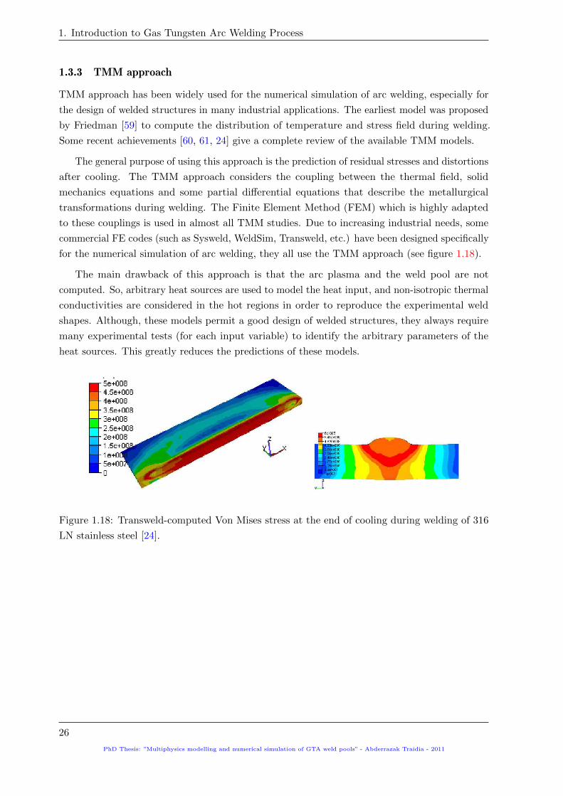
1.3.3 TMM approach
TMM approach has been widely used for the numerical simulation of arc welding, especially for
the design of welded structures in many industrial applications. The earliest model was proposed
by Friedman [59] to compute the distribution of temperature and stress field during welding.
Some recent achievements [60, 61, 24] give a complete review of the available TMM models.
The general purpose of using this approach is the prediction of residual stresses and distortions
after cooling. The TMM approach considers the coupling between the thermal field, solid
mechanics equations and some partial differential equations that describe the metallurgical
transformations during welding. The Finite Element Method (FEM) which is highly adapted
to these couplings is used in almost all TMM studies. Due to increasing industrial needs, some
commercial FE codes (such as Sysweld, WeldSim, Transweld, etc.) have been designed specifically
for the numerical simulation of arc welding, they all use the TMM approach (see figure 1.18).
The main drawback of this approach is that the arc plasma and the weld pool are not
computed. So, arbitrary heat sources are used to model the heat input, and non-isotropic thermal
conductivities are considered in the hot regions in order to reproduce the experimental weld
shapes. Although, these models permit a good design of welded structures, they always require
many experimental tests (for each input variable) to identify the arbitrary parameters of the
heat sources. This greatly reduces the predictions of these models.
Figure 1.18: Transweld-computed Von Mises stress at the end of cooling during welding of 316
LN stainless steel [24].
26
PhD Thesis: ”Multiphysics modelling and numerical simulation of GTA weld pools” - Abderrazak Traidia - 2011

Part I
Study of spot Gas Tungsten Arc Welding:
a 2D modelling
PhD Thesis: ”Multiphysics modelling and numerical simulation of GTA weld pools” - Abderrazak Traidia - 2011
27


Chapter 2
Study of the weld pool dynamics in
pulsed current welding
This chapter deals with the numerical simulation of the weld pool
dynamics under pulsed current welding. A transient
two-dimensional model is developed to analyse the weld pool
formation during welding. The influence of pulsed welding
parameters is numerically investigated, and the resulting weld
shapes are compared with experimental macrographs.
Contents
2.1 Mathematical formulation and governing equations . . . . . . . . . . . . . . . . . . 31
2.1.1 Heat transfer and fluid flow . . . . . . . . . . . . . . . . . . . . . . . . . . . 32
2.1.2 Electromagnetic force field . . . . . . . . . . . . . . . . . . . . . . . . . . . . 34
2.1.3 The free surface deformation . . . . . . . . . . . . . . . . . . . . . . . . . . 35
2.1.4 The liquid/solid interface . . . . . . . . . . . . . . . . . . . . . . . . . . . . 38
2.1.5 Summary of equations . . . . . . . . . . . . . . . . . . . . . . . . . . . . . . 39
2.1.6 Geometry and boundary conditions . . . . . . . . . . . . . . . . . . . . . . . 40
2.2 Results and discussion . . . . . . . . . . . . . . . . . . . . . . . . . . . . . . . . . . 42
2.2.1 Analysis of the weld pool behaviour . . . . . . . . . . . . . . . . . . . . . . 43
2.2.2 Effect of operating parameters on the weld pool dynamics . . . . . . . . . . 50
2.2.3 Effect of the free surface deformation . . . . . . . . . . . . . . . . . . . . . . 58
PhD Thesis: ”Multiphysics modelling and numerical simulation of GTA weld pools” - Abderrazak Traidia - 2011
29

2.3 Investigating the asymmetry sources in horizontal-position welding: a 2D model . 62
2.3.1 approach . . . . . . . . . . . . . . . . . . . . . . . . . . . . . . . . . . . . . 62
2.3.2 Results . . . . . . . . . . . . . . . . . . . . . . . . . . . . . . . . . . . . . . 63
2.4 Conclusion of the chapter and limits . . . . . . . . . . . . . . . . . . . . . . . . . . 66
30
PhD Thesis: ”Multiphysics modelling and numerical simulation of GTA weld pools” - Abderrazak Traidia - 2011
2.1. Mathematical formulation and governing equations
Purpose of the chapter
Although pulsed current GTA welding has become widespread in the manufacturing industry for
its numerous advantages, it introduces a large number of welding parameters, and difficulties are
often encountered to get the optimal set for a given weld shape. A large number of experimental
tests has to be conducted to study the influence of each pulse parameter on the resulting weld
characteristics. The need for industry to increase productivity and availability of computing
facilities justify the use of numerical simulations to investigate the effects of pulsed welding
parameters on the resulting weld shape.
Some experimental studies were conducted to determine the influence of pulsed current
parameters on the welded joint [2, 35]. An analytical model of the heat flow during pulsed current
welding is also available [62]. However, up to the present, far less work has been conducted on
the numerical simulation of heat transfer and fluid flow in pulsed current GTA welding. Kim and
Na [12] used the finite difference method with curvilinear coordinate system to compute heat
transfer and fluid flow in pulsed current welding of an axisymmetric disk. Wu et al. [38] also
used the finite difference method to deal with the case of a moving torch. But in both cases, no
effort was made to understand the time-dependent behaviour of the weld pool at each phase of
the pulse. Moreover, in industry, the choice of welding parameters during pulsed current welding
is still empirical. Here an effort has been made, to study the influence of the main operating
parameters on the weld dimensions, thermal cycles and temperature gradients.
An axisymmetric finite element model is proposed in this chapter to simulate the fluid flow
and heat transfer in the weld pool under pulsed current conditions. This permits an analysis of
the transient behaviour of the weld pool at different times of the heating operation. The shape
of the deformable free surface is also taken into account in a uni-directional MHD coupling, and
the influence of a full coupling with the free surface deformation is also studied. Finally, the
developed model is used to quantify the effects of pulsed welding parameters on the resulting
weld shape.
2.1 Mathematical formulation and governing equations
In order to simplify the problem and to reduce computing times, the following assumptions are
considered:
• The study is restricted to stationary GTA welding (also called spot GTAW). In this
configuration we can use an axisymmetric coordinate system.
• Most of the available weld pool models consider the molten metal flow to be laminar and
incompressible, due to the small size of the weld pool (see appendix A). This assumption is
also considered in our model.
• Buoyancy force is taken into account using the boussinesq approximation, and the latent
heat of fusion is taken into account.
PhD Thesis: ”Multiphysics modelling and numerical simulation of GTA weld pools” - Abderrazak Traidia - 2011
31

2. Study of the weld pool dynamics in pulsed current welding
• The surface tension gradient is dependent on both temperature and sulfur content of the
alloy using the Sahoo et al. relationship.
• The coupling between the MHD calculations and the free surface deformation is in one
way; i.e., the free surface shape does not affect the calculated thermal field.
2.1.1 Heat transfer and fluid flow
Based on the above assumptions, the classical incompressible Navier-Stokes equations for a
Newtonian viscous fluid must be considered to get the velocity, pressure and temperature fields.
For a better clarity, we give these equations in their vectorial form as follows:
(1) Conservation of mass
∇ · ~v = 0 (2.1)
(2) Conservation of momentum
ρ
(∂~v
∂t+ ~v · ∇~v
)= ∇ ·
(−pI + µ(∇~v +∇t~v)
)+ ~Fv (2.2)
(3) Conservation of Energy
ρCp∂T
∂t+ ρCp~v · ∇T = ∇ · (k∇T ) +Qv + ρLf
dfLdt
(2.3)
In equation 2.2, ~Fv represents body forces in the weld pool, it is the sum of Lorentz force and
gravity force, and can be expressed as:
~Fv = ~Fg +−→j ∧−→B (2.4)
where−→j is the current density,
−→B is the magnetic flux density and ~Fg is the gravity force. The
latter is the sum of the inertia force and the buoyancy force, and is expressed as follows (using
the boussinesq approximation):
~Fg = ~Fi + ~Fb
= ρ0−→g − ρ0β(T − Tref )−→g
(2.5)
where ~v is the velocity field in the weld pool, ρ0 is a reference density, β is thermal expansion, g
is gravity, Tref is a reference temperature in the weld pool (taken as the solidus temperature by
some authors [8] and as the liquidus temperature by others [20]).
In the energy conservation equation 2.3, Qv, fL and Lf are respectively the volumetric heat
sources in the weld pool, the liquid fraction and the latent heat of fusion.
Concerning the volumetric heat source in GTAW, it corresponds to the joule effect expressed
using the well known relationship ~Qv = ~j · ~E. However, it has been reported in the literature
that the contribution of the Joule effect is negligible in the weld pool [1].
32
PhD Thesis: ”Multiphysics modelling and numerical simulation of GTA weld pools” - Abderrazak Traidia - 2011

2.1. Mathematical formulation and governing equations
As regards the liquid fraction fL, it is assumed to vary linearly with temperature in the
mushy zone as follows[12]:fL = 1 ; if T > TL
fL =T − TsTL − Ts
; if Ts ≤ T ≤ TL
fL = 0 ; if T < Ts
(2.6)
The equation of energy conservation 2.3 could also be written as:
ρCeqp
(∂T
∂t+ ~v.∇T
)= ∇ · (k∇T ) +Qv (2.7)
where T is temperature, Cp is specific heat and Ceqp = Cp + LfdfLdT
is an equivalent specific heat,
which takes into account the latent heat of fusion Lf .
Formulating the thermal problem using Ceqp is very interesting, since the resulting conservation
equation 2.7 takes the same form as the classical conservation equation. Therefore, it allows the
use of classical Partial Differential Equations solvers.
Conversion to dimensionless form
In order to avoid round-off errors due to manipulations with large/small numbers, it is useful to
rewrite all the governing equations in a dimensionless form. One must define reference quantities
and related scales for time, pressure, length, temperature and velocity. Then, we can introduce
new dimensionless variables for the problem as follows:
R =r
Lref; Z =
z
Lref
V =~v
Vref; τ =
tVrefLref
P =p
ρV 2ref
; Θ =T − T0
TL − Ts
(2.8)
where R and Z are the new dimensionless space coordinates, τ is dimensionless time, and Θ,
V and P are respectively the dimensionless temperature, fluid velocity and pressure fields. As
typical weld pool dimensions are of few millimetres, and the fluid velocity field is around 1 m
s−1, we consider in this study Lref=1 mm and Vref= 1 m s−1.
Based on the above considerations, and assuming a constant value for the molten metal
viscosity µ, the mass, momentum, and energy conservation equations 2.1, 2.2, 2.7 can be rewritten
using the Reynolds number Re =ρVrefLref
µ, as follows:
∇ ·V = 0(∂V
∂τ+ V.∇V
)= −∇P +
1
Re∆V +
LrefρV 2
ref
~Fv
ρCeqp LrefVref
(∂Θ
∂τ+ V∇Θ
)= ∇ · (k∇Θ)
(2.9)
It should be noted that the above dimensionless equation system takes the same form as the
original system, therefore it can be solved by the same classical solvers.
PhD Thesis: ”Multiphysics modelling and numerical simulation of GTA weld pools” - Abderrazak Traidia - 2011
33

2. Study of the weld pool dynamics in pulsed current welding
2.1.2 Electromagnetic force field
The additional resolution of an electromagnetic problem is needed to get the current density and
magnetic flux density distributions. These two vectorial quantities are required to compute the
Lorentz force ~j ∧ ~B that partially governs the molten metal flow. To achieve this, it is important
to note some of the fundamental laws of electromagnetism:
The Ampere’s law: ∇× ~B = µ0~j + µ0ε0
∂ ~E
∂t
The Faraday’s law: ∇× ~E = −∂~B
∂t
The Gauss’s law: ∇ · ~E =Q
ε0Conservation of magnetic flux: ∇ · ~B = 0
(2.10)
where ~B is the magnetic flux density, ~E is the electric field, ~j is the current density, σ is electrical
conductivity, Q is the total electric charge, µ0 and ε0 are respectively vacuum permeability and
vacuum permittivity. It has been well reported for arc welding, that the displacement current
ε0∂ ~E
∂tis negligible compared to the electric current density ~j [1]. Therefore, the Ampere’s law
can be reduced to its stationary form as following:
∇× ~B = µ0~j (2.11)
From the above equations and considering the quasi-neutrality assumption, we get the well known
current continuity equation:
∇ ·~j = 0 (2.12)
A set of equations giving the relationships between the electromagnetic quantities must be added
to the previously given equations system 2.10 as follows:The generalised Ohm’s law: ~j = σ ~E + σ~v × ~B
Relationship between ~B and magnetic potential ~A: ~B = ∇× ~A
Relationship between ~E and electric potential V : ~E = −∇V − ∂ ~A
∂t
(2.13)
where ~v in the above system represents the molten pool velocity field. It has been demonstrated
in the literature, that Ohm’s law can be reduced to ~j = σ ~E, since the relative importance of the
electric effect σ ~E to the convective effect (σ~v × ~B) is in the order of 103 [1].
Considering the reduced Ampere’s equation 2.11, Faraday’s equation 2.10 and the mathe-
matical relationship: ∇×∇× (X) = ∇(∇ ·X) −∆X, we obtain the following equation that
depends only on the magnetic flux density ~B:
∂ ~B
∂t− 1
σµ0∆ ~B = ~0 (2.14)
Since we consider an axisymmetric configuration, only the θ-component of the magnetic flux
density ~B, and the r and z components of the current density ~j are considered. Thus equation
34
PhD Thesis: ”Multiphysics modelling and numerical simulation of GTA weld pools” - Abderrazak Traidia - 2011

2.1. Mathematical formulation and governing equations
2.14 becomes:
∂Bθ∂t
+1
r2µ0σBθ −
1
µ0σ∆Bθ = 0 (2.15)
The above equation is used for the calculation of the azimuthal component of the magnetic
flux density, then the current density vector components are obtained from the simplified equation
of the Ampere’s law 2.11, as follows:
Jr =−1
µ0
∂Bθ∂z
; Jz =1
µ0r
∂(rBθ)
∂r(2.16)
It should be noted that formulating the electromagnetic problem as a function of the magnetic
flux density ~B is very interesting, because the current density ~j is directly obtained by a spacial
differentiation. Indeed, the classical formulation of the electromagnetic problem in terms of the
electric potential V implies an integration step of the current density ~j to obtain the magnetic
flux density ~B, which is more time consuming.
2.1.3 The free surface deformation
Under the actions of the gravitational force, arc pressure and surface tension acting on the weld
pool, the free surface of the molten metal is deformed. Even though, the magnitude of this
deformation is directly linked to the welding current and arc voltage, it has been reported to be
relatively small during GTAW, compared to that of other welding processes, such as GMAW
(where the impact of droplets significantly deforms the free surface of the molten pool) [63]. For
this consideration we assume the free surface as ’flat’ for the MHD calculations. However, we
will compute at each time step the free surface shape in a one-way coupling with the MHD
calculations, so as to validate the assumption of ’flat’ top surface.
z
y
gravity
z=φ(x,y)
O
SL
Figure 2.1: A schematic representation of the free surface deformation.
Figure 2.1 shows a schematic representation of the studied configuration. To be coherent
with the studies available in the literature the z-axis is directed toward the bottom side of the
PhD Thesis: ”Multiphysics modelling and numerical simulation of GTA weld pools” - Abderrazak Traidia - 2011
35

2. Study of the weld pool dynamics in pulsed current welding
workpiece. This is worth noting, since it has an influence on the signs of the different terms
appearing in the equations of the free surface model.
It has been well reported, that the free surface deformation φ(x, y) is the solution of a
variational problem, in which the total potential energy of the surface Et has to be minimised
[44]. This energy is the sum of the surface deformation energy Ed, the gravitational potential
energy Ep and the arc pressure energy Ea.
The surface deformation energy is linked to the curvature of the free surface, and can be
expressed as follows:
Ed =
∫∫St
γ(√
1 + φ2x + φ2
y − 1)
dxdy (2.17)
where St is the top surface of the workpiece projected in the (x,y) plane. γ is the surface tension
of the molten metal, which is set to a quite large value outside the molten area (T < TL) so as to
ensure that the solid zone does not deform (φ = 0).
For the configuration shown in figure 2.1, where the z-axis is descendant, the gravitational
potential energy Ep of the volume V located below the free surface φ can be calculated as follows:
Ep = −∫∫∫
Vρ~g · ~OM dV
= −∫∫∫
Vρ(g~z) · (x~x+ y~y + z~z) dV
= −∫∫∫
Vρgz dV
= −∫∫
St
[∫ 0
φ(x,y)ρgz dz
]dxdy
=
∫∫St
1
2ρgφ2 dxdy
(2.18)
For the configuration shown in figure 2.1, the arc pressure energy Ea is the opposite of the
work performed by the arc pressure force Wa and is given as follows:
Ea = −Wa
= −∫∫
St
(Parc~z) · (φ~z) dxdy
= −∫∫
St
Parcφ dxdy
(2.19)
The total energy of surface Et is finally formulated as follows:
Et = Ed + Ep −Wa
=
∫∫St
γ(√
1 + φ2x + φ2
y − 1)
dxdy +
∫∫St
1
2ρgφ2 dxdy −
∫∫St
Parcφ dxdy
=
∫∫St
F (x, y, φ, φx, φy) dxdy
(2.20)
where g is the positive gravity constant, Parc is the arc pressure (positive value), and φx and
φy are respectively∂φ
∂xand
∂φ
∂y. Without filler metal, the total volume of the molten pool must
36
PhD Thesis: ”Multiphysics modelling and numerical simulation of GTA weld pools” - Abderrazak Traidia - 2011

2.1. Mathematical formulation and governing equations
be conserved, thus the minimisation problem must take into account the following conservation
equation: ∫∫St
φ dxdy =
∫∫St
G(φ) dxdy = 0 (2.21)
Finding the solution φ(x, y) that minimizes the physical quantity Et (equation 2.20) and respects
the constraint expressed in equation 2.21 requires the use of variational calculus. By applying
the Euler-Lagrange criterion, we get:
∂
∂φ(F + λG)− ∂
∂x
[∂
∂φx(F + λG)
]− ∂
∂y
[∂
∂φy(F + λG)
]= 0 (2.22)
where λ is a Lagrangian multiplier used to satisfy the conservation constraint 2.21. After
manipulation the previous equation becomes:
− ∂
∂x
γ φx√1 + φ2
x + φ2y
− ∂
∂y
γ φy√1 + φ2
x + φ2y
+ ρgφ = Parc − λ (2.23)
After the development of partial derivatives in equation 2.23, we obtain the following Partial
Differential Equation (PDE):
Parc − λ− ρgφ = −γφxx(1 + φ2
x)− 2φxφy + φyy(1 + φ2y)
(1 + φ2x + φ2
y)32
(2.24)
In the case of a two-dimensional axisymmetric formalism, φ(x, y) becomes φ(r), and equation
2.23 takes the following form:
− ∂
∂r
(γφr√1 + φ2
r
)− 1
r
γφr√1 + φ2
r
+ ρgφ = Parc − λ (2.25)
After manipulation, the corresponding PDE is as follows:
Parc − λ− ρgφ = −γ rφrr + φr(1 + φ2r)
r(1 + φ2r)
32
(2.26)
where φ is the vertical displacement of the top surface of the weld pool, and φr represents∂φ
∂r. λ
is used to satisfy the volume conservation constraint:
∫S
2πφ(r)rdr = 0.
Here, we note that although many authors prefer the use of the developed forms (PDE’s 2.24
and 2.26), the non-developed forms given in equations 2.23 and 2.25 are more adapted to finite
element formulations for the resolution of partial differential equations. In fact, equations 2.23
and 2.25 can be written in the following classical form:
−∇ · (c∇u) + au = f (2.27)
where u is the unknown variable (here, u = φ), c, a and f are identified from equations 2.23 and
2.25, and are as follows:
c =γ√
1 + φ2x + φ2
y
(3D), orγ√
1 + φ2r
(2D)
a = ρg
f = Parc − λ
(2.28)
PhD Thesis: ”Multiphysics modelling and numerical simulation of GTA weld pools” - Abderrazak Traidia - 2011
37

2. Study of the weld pool dynamics in pulsed current welding
2.1.4 The liquid/solid interface
The liquid/solid interface is the contour corresponding to the liquidus temperature. The main
numerical methods used in weld pool models to track this interface can be classified into two
categories; the moving grid methods, and the fixed grid methods.
The moving grid methods
The moving grid methods permit tracking of the liquid/solid interface with time to create two
different subdomains at each time step, corresponding to the molten metal zone and to the solid
zone. This permits not only use of appropriate physical properties for each zone, but also solution
of the momentum conservation equation only in the liquid zone (which should considerably reduce
the number of degrees of freedom). For instance, a hydrodynamic problem solved in a moving
grid framework, and taking into account the latent heat of fusion, is formulated as follows [24]:
In the liquid domain ΩL(t)
∇ · ~v = 0
ρL
(∂~v
∂t+ ~v · ∇~v
)= −∇p+ µL∆~v + Fv
ρLCpL
(∂T
∂t+ ~v · ∇T
)= ∇ · (k∇T )
In the solid domain Ωs(t)
ρsCps∂T
∂t= ∇ · (k∇T )
Along the solid/liquid interface Γ(t)
~v = ~0
ks∂T
∂n− kL
∂T
∂n= ρLfvn
(2.29)
where ∂ · /∂n is the normal derivative with respect to the solid/liquid interface Γ(t), Lf is the
latent heat of fusion and vn is the velocity normal to Γ(t).
For moving grid methods, the mesh (grid) is generated at each time step according to the
current location of Γ(t). At each mesh generation, one must ensure that a line (2D problems), or a
surface (3D problems) of the generated grid is coincident with Γ(t). A coordinate transformation
technique is often used in moving grid simulations. This permits the solution of an adjunct
problem on a regular grid coordinate system rather than on the original problem on the deformed
grid.
The main advantage of moving grids methods, is that different physics can be solved separately
in each area (liquid or solid). However, generating a new grid at each time step depending on
the liquid/solid interface is quite difficult, and time consuming.
38
PhD Thesis: ”Multiphysics modelling and numerical simulation of GTA weld pools” - Abderrazak Traidia - 2011

2.1. Mathematical formulation and governing equations
The fixed grid methods
In fixed grid methods, the computational mesh is only generated once, and the liquid/solid
interface is located using the liquid fraction function fL(T ). Contrary to the moving grid methods,
here, all the governing equations are computed in the whole domain (liquid and solid zones).
In order to use different physical properties for each zone, we can use the liquid fraction fL as
follows:
α = αLfL + αs(1− fL) (2.30)
where α is the considered physical property, and αL and αs are respectively the physical properties
for the liquid and solid phases.
In fixed grid methods, as the momentum equation is also computed in the whole domain, one
must ensure that the velocity field is zero in the solid region. To achieve this, two main methods
are used: the Karman-Kozeny approximation [64], and the enhanced viscosity method.
The Karman-Kozeny approximation which is derived from the Darcy law [64], has been widely
used in most fixed grid weld pool models. The idea is to introduce a new source term ~Su in the
momentum conservation equation 2.2, to account for the frictional dissipation in the mushy zone,
as follows:
~Su = −C (1− fL)2
f3L +B
~v (2.31)
where C is a relatively huge constant (in the order of 1010) that ensures the decrease of the velocity
field in the solid region, and B is a relatively low constant (in the order of 10−3) introduced to
avoid division by zero.
The second method consists in increasing the dynamic viscosity appearing in the momentum
conservation equation 2.2 in the solid area. This is done either by using a Heaviside function, or
directly by using the liquid fraction fL as follows:
µ = µL(T )fL + µs(1− fL) (2.32)
where µL(T ) is the liquid dynamic viscosity (that could vary with temperature), and µs is an
artificial solid viscosity, which is high enough such that fluid flow is completely stopped in the
solid zone.
We tested the two previously described methods on a simple melting/solidification configura-
tion, and we concluded that they give very close results in terms of fluid velocity and weld shape.
However, the enhanced viscosity was found to be less time consuming and is used in the present
work.
2.1.5 Summary of equations
As presented previously, the equations of the problem are solved in a dimensionless form. However,
for clarity, a summary of equations to be solved is given in its dimensioned form as follows:
PhD Thesis: ”Multiphysics modelling and numerical simulation of GTA weld pools” - Abderrazak Traidia - 2011
39

2. Study of the weld pool dynamics in pulsed current welding
Equations to be solved in the subdomains:
∇ · ~v = 0
ρ
(∂~v
∂t+ ~v · ∇~v
)= −∇p+ µ∆~v + ρ0(1− β(T − Tref ))−→g +
−→j ×−→B
ρCeqp
(∂T
∂t+ ~v · ∇T
)= ∇ · (k∇T )
∂Bθ∂t
+1
r2µ0σBθ −
1
µ0σ∆Bθ = 0
~j =1
µ0∇× ~B
(2.33)
Equation to be solved at the top free surface:
Parc − λ− ρgφ = −γ rφrr + φr(1 + φ2r)
r(1 + φ2r)
32
with λ used to verify:
∫St
2πφ(r)rdr = 0
(2.34)
2.1.6 Geometry and boundary conditions
Figure 2.2 shows the computational domain used in this study. In order to reduce computing
times, the geometry is made of two subdomains with different mesh densities in each subdomain.
In particular, the electromagnetic and energy conservation equations are solved in the whole
domain; i.e., AEFG with a relatively coarse mesh. The momentum and mass conservation
equations are only solved in the subdomain ABCD with a finer mesh size (about 200 µm). At
the top surface AB where high gradients of temperature and velocity occur, a finer mesh size
must be considered (about 50 µm).
Figure 2.2: Computational domain used for the study of stationary pulsed current GTAW.
The resolution of the equations system 2.33, requires the addition of some boundary conditions
formulated as functions of the unknown variables; (u, v, p, T , Bθ, φ). In the case of partially
penetrated weld pools (figure 2.2 left) the boundary conditions of the problem are listed as
follows:
40
PhD Thesis: ”Multiphysics modelling and numerical simulation of GTA weld pools” - Abderrazak Traidia - 2011

2.1. Mathematical formulation and governing equations
(1) At the top surface of the workpiece (AB+BE)
Input heat flux and current density are imposed:
~j · (~n) = Jz =1
µ0r
∂(rBθ)
∂r= J0(r)⇐⇒ ∂(rBθ)
∂r= µ0rJ0(r)
~q · (−~n) = k∂T
∂z= q0(r)
φ = 0 if T 6 TL
φr = 0 at r = 0
(2.35)
where j0(r) and q0(r) are respectively the current density and heat flux at the top surface of the
workpiece. They are assumed to be in Gaussian distributions as presented in the first chapter
(see equation 1.5). Here, the parameters of the Gaussian distributions are: d=3 (usually the
case for GTAW [43]) and η=0.68 [43]. We considered rH = rJ and varying between 4 and 5 mm
depending on the welding current, as reported in table 2.1. The value of the voltage for each
current was identified experimentally (set-up described further) and reported also in table 2.1.
In addition, at the boundary AB, the normal velocity is zero and the Marangoni shear stress
must be considered. As the free surface of the weld pool is assumed to be ’flat’ for the fluid flow
calculation, the Marangoni condition presented in the first chapter (see equation 1.3) is simplified
as follows: µ∂u
∂z= fL
∂γ
∂T
∂T
∂rv = 0
(2.36)
where u and v are respectively radial and axial velocity components.
In this study, the surface tension gradient∂γ
∂Tis taken to be dependent on temperature and
sulfur content using the Sahoo et al. [19] relationship, reminded below:
∂γ
∂T= −Aγ −RgΓs ln(1 +Kas)−
Kas1 +Kas
Γs∆H0
T
K(T ) = k1 exp(−∆H0
RgT)
(2.37)
Welding current (A) Arc Voltage (V) rH (mm)
80 12.6 4.2
100 12.7 4.4
120 13.2 4.7
160 14.3 5
180 14.5 5
100 15 5
Table 2.1: Heat source parameters used for the different simulations.
(2) At the outer surface (EF)
PhD Thesis: ”Multiphysics modelling and numerical simulation of GTA weld pools” - Abderrazak Traidia - 2011
41

2. Study of the weld pool dynamics in pulsed current welding
A convective heat dissipation is considered:~q · (~n) = −k∂T
∂r= h0(T − T0)
Jz = 0⇐⇒ ∂(rBθ)
∂r= 0
(2.38)
(3) At the bottom surface (FG)
A convective heat dissipation and electric insulation are considered:~q · (~n) = k
∂T
∂z= h0(T − T0)
Jz = 0⇐⇒ ∂(rBθ)
∂r= 0
(2.39)
(4) Along the axis of symmetry (AD+DG)
The normal heat flux, normal velocity and the magnetic field are set to zero:~q · (~n) = 0
Bθ = 0
u = 0
(2.40)
(5) Along the solid interfaces (BC+CD)
The velocity components are set to zero
u = v = 0 (2.41)
2.1.6.1 Numerical procedure
Comsol Multiphysics software is used to solve all the coupled multiphysics equations. All the
governing equations are rewritten in their weak forms, and solved by the UMFPACK Direct
Solver. It solves general systems of the form Ax = b using the nonsymmetric-pattern multifrontal
method and direct LU factorisation of the sparse matrix A. For the time integration method, we
use the Backward Differentiation Formula (BDF), which is a robust method that is commonly
used for a wide range of problems. Calculations are performed within some 20 minutes, on 2.6
GHz CPU speed and 2.5 Gb RAM memory computer.
2.2 Results and discussion
This section is divided into two parts:
In the first part, we present the results of the developed model for partially penetrated weld
pools, with particular attention given to the analysis of the weld pool behaviour at each period
of the pulse. We also compare welding under constant current with pulsed current and try to
emphasize the reported benefits of the PC GTAW mode, and finally we show the influence of a
self-consistent calculation of the free surface deformation on the computed results.
The second part will be dedicated to understanding the effects of operating parameters such as
42
PhD Thesis: ”Multiphysics modelling and numerical simulation of GTA weld pools” - Abderrazak Traidia - 2011
2.2. Results and discussion
current ratio (Ip/Ib), pulse frequency and peak pulse duration on the weld pool dynamics and
weld shapes.
The numerical model is applied to AISI 304 stainless steel containing 0.0072 wt% sulfur.
Table 2.2 lists the physical properties of this alloy taken from literature.
Symbol Nomenclature Value
Tl Liquidus temperature 1723 K [12]
Ts Solidus temperature 1673 K [12]
Tref Reference temperature 1723 K
ρl Liquid phase density 6350 kg m−3 [65]
ρs Solid phase density 7500 kg m−3 [65]
ρ0 Reference density 6350 kg m−3
Cpl Specific heat of liquid phase 720 J kg−1 K−1 [65]
Cps Specific heat of solid phase 602 J kg−1 K−1 [65]
kl Thermal conductivity of liquid phase 20 W m−1 K−1 [65]
ks Thermal conductivity of solid phase 26 W m−1 K−1 [12]
h0 Heat convection coefficient 15 W m−2 K−1
µ Dynamic viscosity of liquid phase 0.05 kg m−1 s−1 [12]
σ Electrical conductivity 7.7×10⁵ Ω−1 m−1 [12]
Lf Latent heat of fusion 2.47 ×10⁵ J Kg−1 [12]
as Activity of sulfur 0.0072 wt%
Aγ Constant in surface tension gradient 3×10⁻⁴ N m−1 K−1
Rg Gas constant 8314.3 J kmol−1 K−1 [12]
∆H0 Standard heat of adsorption -1.88×10⁸ J kmol−1 [12]
Γs Surface excess at saturation 1.3×10⁻⁸ kmol m−2 [12]
γm Surface tension at pure metal 1.943 N m−1 [12]
k1 Entropy factor 3.18×10⁻³ ([19])
Ip Peak pulse current 200 A
Ib Background current 80 A
tp Peak pulse duration 0.25 s
tb Background duration 0.25 s
f Pulse frequency 2 Hz
tt Total heating duration 3.5 s
np Total number of periods 7
Table 2.2: Material properties of AISI 304 stainless steel, and pulsed welding parameters
2.2.1 Analysis of the weld pool behaviour
In this part, we study the time evolution of the weld pool for a 10 mm thick disk. The operating
parameters are listed in table 2.2.
PhD Thesis: ”Multiphysics modelling and numerical simulation of GTA weld pools” - Abderrazak Traidia - 2011
43

2. Study of the weld pool dynamics in pulsed current welding
2.2.1.1 The weld pool dynamics
It is well known that the fluid flow and heat transfer in the weld pool are dominated by the
Marangoni convection, which is due to the temperature gradient of surface tension∂γ
∂T. For
a 72 ppm sulfur content steel, the evolution of the surface tension gradient with temperature
is given in figure 2.3. Analysing this figure, shows that∂γ
∂Tis positive until temperature
reaches approximately a critical temperature Tc = 2300 K, it then becomes negative for higher
temperatures.
Figure 2.3: Surface tension gradient as function of temperature for a 72 ppm sulfur content AISI
304 stainless steel.
Figures 2.4 and 2.5 show the time evolution of the simulated weld pool at the end of each
background time and each peak time for the total heating duration. In each figure the normalized
velocity field and the streamlines inside the molten pool are represented to identify vortices, as
well as the weld shape (total molten zone) at the considered time.
First it is important to notice that at each time, it clearly appears two vortices; a clockwise
vortex near the center of the weld pool inducing an outward fluid flow at the surface, and a
counter-clockwise vortex near the edges of the weld pool inducing an inward fluid flow. It is
also seen that at each background time the counter-clockwise vortex is clearly dominant, which
induces a deep and narrow weld pool, whereas, at each peak time the clockwise vortex is dominant
which creates a wide and shallow weld pool. This ’alternate domination’ of each vortex creates
a dynamic effect leading to an alternate evolution of the weld characteristics. In other words,
the final weld shape must be determined by the whole welding cycle, and does not necessarily
correspond to the molten zone at the last time of heating, since the interesting fact here is
that: the weld width is increased during the peak time, while the depth is increased during the
background time.
44
PhD Thesis: ”Multiphysics modelling and numerical simulation of GTA weld pools” - Abderrazak Traidia - 2011

2.2. Results and discussion
Figure 2.4: Time evolution of the weld pool (T = TL), normalized velocity and re-solidified metal
(white), for a 80/200 A pulsed current during the four first periods.
PhD Thesis: ”Multiphysics modelling and numerical simulation of GTA weld pools” - Abderrazak Traidia - 2011
45

2. Study of the weld pool dynamics in pulsed current welding
Figure 2.5: Time evolution of the weld pool (T = TL), normalized velocity and re-solidified metal
(white), for a 80/200 A pulsed current during the three last periods
Figure 2.6: Surface temperature distribution at the last background time t=3.25 s.
46
PhD Thesis: ”Multiphysics modelling and numerical simulation of GTA weld pools” - Abderrazak Traidia - 2011

2.2. Results and discussion
Figure 2.7: Surface temperature distribution at the last peak time t=3.5 s.
This ’alternate domination’ phenomenon is explained by the change in the sign of∂γ
∂T, and
more precisely by the change in the location of the surface point where T = Tc. Indeed, as seen in
figure 2.6, at background time the temperature varies from the liquidus temperature TL = 1723
K to about Tmax = 2650 K, which is above the critical temperature Tc shown previously in figure
2.3. This explains the existence of two vortices; a clockwise one corresponding to the region where∂γ
∂T< 0 and a counterclockwise vortex corresponding to the domain where
∂γ
∂T> 0. Additionally,
as the surface point where T = Tc is close to the weld axis, the region where∂γ
∂T> 0 is larger
than that where∂γ
∂T< 0, which explains the domination of the counter-clockwise vortex.
However, at peak time, figure 2.7 shows that Tmax is above 3000 K and the surface point
where T = Tc is located far from the weld axis, then the region where∂γ
∂T< 0 is much more
important than the region where∂γ
∂T> 0. This leads to the domination of the clockwise vortex
during the peak time duration.
In other words the ’alternate domination’ of vortices corresponds simply to a cyclic change in
the location of the surface point where temperature equals the critical temperature Tc.
It is obvious that this dynamic effect has strong consequences on the weld pool dimensions.
The time evolution of the weld pool depth and half-width is given in figure 2.8. As seen in this
figure, the weld pool dimensions present very clear changes at each peak or background time,
which perfectly illustrates the domination of each vortex, discussed above. Since the clockwise
vortex is dominant at peak time, the outward fluid flow at the top surface increases the weld
pool width, while its depth is decreasing. Conversely, during the background time, the width is
decreasing while the depth is increasing which illustrates the domination of the counter-clockwise
vortex.
The velocity field at the top surface of the weld pool plays an important role for the heat
PhD Thesis: ”Multiphysics modelling and numerical simulation of GTA weld pools” - Abderrazak Traidia - 2011
47

2. Study of the weld pool dynamics in pulsed current welding
transfer inside the molten pool. Figure 2.9 plots the evolution of the radial velocity u as function
of the radius r at the top surface. The two curves are plotted at the end of the peak and
background times for the last heating period. As it was predicted, in each curve there are two
regions corresponding to the two vortices; one region in which the radial velocity is negative, the
other one corresponding to a positive velocity. During the background time the radial velocity
is predominantly negative with a maximum of 35 cm s−1, this velocity becomes predominantly
positive during the peak time with a maximum of 40 cm s−1.
Figure 2.8: Time evolution of the weld pool dimensions.
Figure 2.9: Radial velocity at the top surface of the weld pool at the last period of heating.
Figure 2.10 shows the free surface shape at the last background time (current=80 A), and
48
PhD Thesis: ”Multiphysics modelling and numerical simulation of GTA weld pools” - Abderrazak Traidia - 2011

2.2. Results and discussion
the last peak time (current=200 A). The free surface is clearly deformed under the action of arc
pressure, gravity and surface tension. The maximum depression reached for the peak current
is about 0.28 mm whereas it is about 0.09 mm for the background current. These values are
very small compared to the weld pool dimensions, which is consistent with the one side coupling
considered between the free surface deformation and the hydrodynamics computations. The
influence of a strong coupling between the deformed free surface and the fluid flow calculus will
be presented later.
Figure 2.10: Free surface shapes at the last peak and background times.
2.2.1.2 Comparison between constant and pulsed current welding
The considered pulsed current welding (80/200 A, 2 Hz) is here compared to a constant current
welding which produces approximately the same weld pool geometry (depth and width). This will
demonstrate the ability of pulsed welding to produce the same penetration as a constant current
welding, but with less energy. Then, we will expect to have less distortions of the assembly with
pulsed current welding.
Figure 2.11 presents the time evolution of the weld pool half-width and depth for spot welding
of a 10 mm thick disk. Three different cases are presented; a pulsed current welding of (80/200
A, 2 Hz), a continuous current welding that represents the mean current between 80 A and 200 A
which is 140 A, and a continuous current welding of 170 A. First, we note that during the whole
welding cycle, the pulsed current case produces a deeper and wider weld pool than the continuous
mean current (140 A). This is in a good agreement with what has been reported experimentally
in the literature. Moreover, it clearly appears that to produce nearly the same weld as the pulsed
current, one needs to increase the continuous current from 140 to 170 A. However, in term of
energy, over 3.5 s the 170 A continuous current corresponds to a total heating energy of 5867
J, while the pulsed current is equivalent to 4565 J, so the increase in the energy is significant
(around 30%).
PhD Thesis: ”Multiphysics modelling and numerical simulation of GTA weld pools” - Abderrazak Traidia - 2011
49

2. Study of the weld pool dynamics in pulsed current welding
In other words, for a given weld pool shape (width and depth) we reduce the welding energy
by 30 % (and the welding current by 22 %) when using pulsed current welding. Then the residual
stresses and distortions are expected to be significantly reduced.
Figure 2.11: Comparison of weld pool dimensions between constant and pulsed current welding.
2.2.2 Effect of operating parameters on the weld pool dynamics
The aim of welders is to select the best welding parameters to maximise welding penetration
and to minimize thermal gradients (to reduce distortions). Pulsed current welding is then an
optimal choice. However, the welding parameters are more complex to define, and up to date,
the choice of parameters remains empirical and based on experimental tests. In this section, we
will use our model to understand the influence of the three main parameters of the pulse; i.e.,
the current ratio, the pulse frequency and the peak pulse duration, on the weld pool shape and
thermal gradients.
2.2.2.1 Influence of the current ratio at constant energy
Here, we study at constant welding energy, and with a 140 A mean current, three different
current variations; (120/160 A), (100/180 A) and (80/200 A). The influence of each current
variation on the resulting weld pool shape and the corresponding thermal field distribution are
investigated. Figure 2.12 shows the time evolution of welding currents and the experimentally
measured voltage for each case (arc length set to 5 mm). In order to understand the effects of
only the current ratio Ip/Ib, the three studied cases have the same pulse frequency (2 Hz), and
the peak pulse duration tp is equal to the background duration tb. Simulated weld shapes after
solidification for the three cases are compared to experimental macrographies.
50
PhD Thesis: ”Multiphysics modelling and numerical simulation of GTA weld pools” - Abderrazak Traidia - 2011

2.2. Results and discussion
Figure 2.12: Three current evolutions at constant energy (left), and the corresponding measured
voltages (right).
The time evolution of the weld pool half-width and depth for the three welding cases is given
in figure 2.13, in which the case of the continuous mean current of 140 A is also represented for
comparison. The first remarkable observation is that the three pulsed cases produce a deeper
and wider weld pool than the mean current case. This suggests saying that for a given level of
welding energy, it is more interesting to use a pulsed current welding than a constant current one.
Figure 2.13: Time evolution of the weld pool dimensions, for different welding current distribu-
tions.
As concerns the pulsed cases, we notice that the depth difference between the three current
distributions is higher than the width difference. Moreover, it is found that the 80/200 A case
produces a deeper and wider weld pool than the other cases. This result is explained by the fact
PhD Thesis: ”Multiphysics modelling and numerical simulation of GTA weld pools” - Abderrazak Traidia - 2011
51

2. Study of the weld pool dynamics in pulsed current welding
that the ’alternate domination’ of vortices studied previously, is much more important when the
gap between the peak and background currents is high.
To illustrate this idea, we shall define a variable that quantifies the magnitude of the
’alternate domination’ phenomenon for each current distribution. Consider Rd/w(t), defined as
Rd/w(t) =d(t)
w(t), where d(t) is the weld pool depth at time t, and w(t) is the weld pool half-width
at the same time. It is obvious that time variations in Rd/w(t) are caused by two effects:
• Effect of pulsing the heat source. In this case w(t) and d(t) should evolve with time in the
same directions, as shown in figure 2.14; i.e., when w(t) increases, d(t) increases, and vice
versa. This would induce ’small’ oscillations in the time evolution of Rd/w(t)
• Effect of the ’alternate domination’ of vortices. In this case w(t) and d(t) will evolve with
time in opposite directions, as shown in figure 2.14; i.e., when w(t) increases, d(t) decreases,
and vice versa. This would induce ’strong’ oscillations in the time evolution of Rd/w(t)
By considering the above discussion, ’small’ oscillations in the time evolution of Rd/w(t)
means that the alternate domination phenomenon is not so important and oscillations are mainly
due to the pulsing of the heat source. However, ’strong’ oscillations in Rd/w(t) means that the
’alternate domination’ phenomenon is quite important.
Figure 2.14: Effect of pulsing the heat source and the ’alternate domination’ of vortices on the
variation of the weld pool dimensions.
Figure 2.15 shows the time evolution of Rd/w(t) for the three studied cases, and as expected,
strong oscillations are observed in the (80/200 A) curve. This is the consequence of the high gap
between the peak and background currents. Indeed, during the background time, as the welding
current is too low (80 A) the temperature at the top surface is not so high, which leads to a large
region with positive surface tension gradient, and results in a strong domination of the clockwise
vortex. This induces a high drop in Rd/w(t), as seen in figure 2.15. However, during the peak
time, as the welding current is high (200 A), the surface temperature of the weld pool is much
more important, and causes a large region with negative surface tension gradient. Consequently,
this induces a strong domination of the counter-clockwise vortex, which results in a high increase
in Rd/w(t).
52
PhD Thesis: ”Multiphysics modelling and numerical simulation of GTA weld pools” - Abderrazak Traidia - 2011

2.2. Results and discussion
Figure 2.15: Time evolution of Rd/w(t), for different welding current distributions.
Figure 2.16: Surface temperature distributions at the last time of heating (left), and time evolution
of temperature gradients near the edges of the welds (right) for different current distributions.
Concerning the temperature field, the comparison between the three pulsed cases and the mean
current is given in figure 2.16 (left), showing the radial evolution of the top surface temperature
at the last time of heating. As expected the pulsed cases induce a higher temperature at the
center of the plate than the continuous current. The interesting point here, is that far from the
molten pool, there is no difference between all cases. This is probably due the fact that all cases
have the same welding energy.
As said previously, the pulsed current cases produce a wider and deeper weld pool than the
mean current, however they induce higher thermal gradients caused by the periodic transition
between two levels of current. To emphasize this difference, figure 2.16 (right) shows the time-
PhD Thesis: ”Multiphysics modelling and numerical simulation of GTA weld pools” - Abderrazak Traidia - 2011
53

2. Study of the weld pool dynamics in pulsed current welding
evolution of thermal gradients near the edges of welds for all cases. We choose the edge of the
weld, since it is located in the Heat Affected Zone where the main plastic strains are located. As
seen in this figure, until time t=1 s, the mean current 140 A induces a higher thermal gradient
than the pulsed cases. However thermal gradients tend to stabilize for the mean current after
time t=1 s, while it continues to increase periodically for the three pulsed current cases. Then, an
optimal choice must be made between the weld penetration and the induced thermal gradients.
An experimental validation was handled to reproduce the three numerically studied pulsed
cases. we considered a spot GTA welding of an AISI 304 stainless steel disk (same dimensions as
in simulations), a tungsten electrode (diameter of 3.2 mm with 60 tip angle) was used with a 5
mm arc-length , and argon was used as a shielding gas at a flow rate of 15 L/min. Figure 2.17
shows the comparison between the experimental macrographies of the three pulsed current cases
and the corresponding predicted weld shapes. It shows a good agreement between experiments
and predictions, as much as shape as dimensions. Additionally, as two solidification fronts appear
only on the welds widths, and not on the welds depths, the last time of heating was necessarily a
background time, and it causes the last increase observed in the welds depths. This confirms the
predomination of the inward vortex during the background time, and goes with our numerical
predictions.
Figure 2.17: Comparison between the experimental macrographies and numerically predicted
weld shapes;(a) 80/200 A, (b) 100/180 A, (c) 120/160 A.
2.2.2.2 Influence of the pulse frequency at constant energy
The variation of pulse frequency leads to control the heating period between the bottom and
peak welding currents. Then frequency controls thermal gradients and influences the fluid flow
in the weld pool. Using a 80/200 A pulsed current, with three different frequencies of 2, 4 and 6
Hz, we study the effect of the current frequency on the weld pool variations.
54
PhD Thesis: ”Multiphysics modelling and numerical simulation of GTA weld pools” - Abderrazak Traidia - 2011

2.2. Results and discussion
First, we start by comparing the weld pool depth and width for each frequency. As seen
in figure 2.18 the weld pool characteristics evolve at the same frequency as the corresponding
welding current. As shown previously, during the peak duration the weld pool width increases
while the depth decreases and during the background duration the width decreases while the
depth increases, this observation is valid for all cases.
As regards dimensions, the 2 Hz case produces a wider and deeper weld pool than the other
cases, this is caused by the fact that for the 2 Hz case, both peak and background currents are
held during more time. This provides more time for the predomination of vortices at each peak
and background times, resulting in an increase of the weld dimensions.
Figure 2.18: Time evolution of the weld pool dimensions for different pulse frequencies.
Figure 2.19: Computed weld shapes for the different pulse frequencies.
The computed weld shapes for each frequency are compared in figure 2.19, it goes with the
previous remarks. The comparison between the three cases is very interesting, it shows that
we can get different weld shapes using the same welding energy, simply by changing the pulse
frequency.
PhD Thesis: ”Multiphysics modelling and numerical simulation of GTA weld pools” - Abderrazak Traidia - 2011
55

2. Study of the weld pool dynamics in pulsed current welding
2.2.2.3 Influence of the peak pulse duration
In our previous analysis of the effects of current ratio and pulse frequency on the weld shape, we
assumed that the peak pulse duration equals the background pulse duration; tp = tb. However,
in practice the peak pulse duration tp is set below 50% of the pulse period T , so as to reduce
residual stresses and distortions. In this paragraph, we analyse the effects of three peak pulse
durations on the computed results. We consider the cases of:tpT
= 25%,tpT
= 35% andtpT
= 45%.
It is important to note that when increasing only the peak pulse duration, the welding energy
is also increased. So, to have the same welding energy for the three studied cases, we must reduce
the peak welding current when the peak pulse duration is increased (here we choose to maintain
the same background current for all cases).
Figure 2.20 shows the distribution of welding currents for three studied cases (only one period
is shown). The comparison between the three resulting weld pool dimensions is shown in figure
2.21. It is remarkable to see that even though the peak pulse durations are different, all cases
produce the same weld dimensions. We can even say that, unexpectedly, the lowest casetpT
= 25%
produces a slightly wider weld pool than the two other cases. This interesting fact is due to the
large gap between the peak and background currents for the 25 % case, compared to the other
situations. As this gap is large, the ’alternate domination’ of vortices is more important, and
then leads to production of nearly the same weld as the other cases.
Figure 2.20: Schematic representation for one period of the time evolution of the welding current
for different peak pulse durations at constant energy.
56
PhD Thesis: ”Multiphysics modelling and numerical simulation of GTA weld pools” - Abderrazak Traidia - 2011

2.2. Results and discussion
Figure 2.21: Time evolution of the weld pool dimensions for different peak pulse durations at
constant energy.
2.2.2.4 Importance of the sulfur content
From the previous analysis, it has been shown that the ’alternate domination’ of vortices, plays
an important role in controlling the weld pool dynamics. However, as this phenomenon is caused
by the Marangoni effect, and more specifically by the alternate change in the sign of the surface
tension gradient, the sulfur content of the alloy has a very important impact on the previous
given conclusions.
In this subsection we consider two different sulfur contents (10 ppm, and the previously
studied 72 ppm), and try to see their influence on the ’alternate domination’ effect. It should be
noted that we considered a low sulfur case (10 ppm), since, today most of the stainless steels
used for welding applications are of low sulfur content (because of segregation, cracks, etc.). For
comparing the two cases, the welding parameters are set to (80/200 A, 2 Hz).
Figure 2.22 shows the time evolution of Rd/w(t) , and the predicted weld shapes for the two
studied cases. First, we note that strong oscillations appear in the Rd/w(t) curve of the 72 ppm
case, whereas, it is not the case for the low sulfur content case. This is explained by the fact that
for low sulfur content, the surface tension gradient is negative for all temperatures. Then, only
one counter-clockwise vortex will control the weld pool time evolution, leading to have a wide
and shallow weld pool, as shown in figure 2.22 (right). The strong changes in the Rd/w(t) curve
of the 72 ppm sulfur case means that the ’alternate domination’ phenomenon is quite important.
This leads to the conclusion that when adding sulfur to the weld pool, the critical temperature Tc
shifts toward high temperatures, and then the ’alternate domination’ effect is enhanced, leading
to a wide and deep weld pool, as shown in figure 2.22 (right).
Obviously, a high addition of sulfur would lead to a high increase in the value of Tc, and the
surface tension gradient would be positive at all temperatures. This would reduce considerably
PhD Thesis: ”Multiphysics modelling and numerical simulation of GTA weld pools” - Abderrazak Traidia - 2011
57
2. Study of the weld pool dynamics in pulsed current welding
the benefit of the ’alternate domination’ effect. Consequently, an optimum choice of sulfur content
should be made, so as to take benefit from the presence of two vortices in the weld pool.
Figure 2.22: Evolution of Rd/w(t) and final weld shapes for two different sulfur contents.
2.2.3 Effect of the free surface deformation
The depression of GTA weld pool due to arc pressure was previously calculated by our ax-
isymmetrical model, but not included self-consistently. In other words, a weak coupling was
assumed between the surface deformation and the hydrodynamic calculations. This assumption
was validated by the low values of surface depressions in GTAW compared to GMAW process.
Consequently, the temperature and velocity fields were computed on the initial ’flat’ geometry.
In this subsection, we are interested in studying the effect of a self-consistent calculation
of the free surface depression on the resulting weld shape. To achieve this, we will consider a
disk heated continuously by a constant current, and where the lateral and bottom sides are
maintained at room temperature (to avoid a full penetration). We will focus on the determination
of the steady-state solution for the temperature and velocity fields, as well as the free surface
shape. Two kinds of models will be compared; a model assuming a ’flat’ free surface (which is
the steady-state formulation of the model used in the previous sections), and a model in which
the weld pool surface is computed self-consistently.
2.2.3.1 Ensuring a strong coupling: two approaches
To ensure a two-way coupling between the free surface deformation and the thermohydraulic
calculations, various numerical methods can be used. In this study, we use the Arbitrary
Lagrangian-Eulerian method (a brief description of the ALE method is given in appendix B). By
using this method, a new computational framework is created (named ALE framework), which
permits computing of different fields on a deforming geometry, while the mesh deformation is
itself governed by one (or more) of the computed fields. Two approaches can be used for the
coupling of the thermohydraulic calculations with the ALE framework deformation. These two
methods are briefly described below.
The quasi-static approach
The quasi-static approach consists of deforming the ALE framework using a displacement-
controlled mode. This means that, first the free surface deformation φ is computed by the
minimization of the global energy of the surface (using equation 2.25), and then the ALE
framework is deformed using the transformation z = φ(r) at the top surface. The thermohydraulic
fields are then computed on the newly generated ALE framework. The calculation steps are
summarized as follows:
58
PhD Thesis: ”Multiphysics modelling and numerical simulation of GTA weld pools” - Abderrazak Traidia - 2011

2.2. Results and discussion
(1) Initialisation of the geometry, boundary conditions and input parameters. The current ALE
mesh is set to the initial unreformed mesh. .
(2) Steady-state calculation, on the current ALE mesh, of temperature (T ), fluid velocity
(u, v) and pressure (p) fields (resolution of the system of equations 2.9 in its steady-state
formulation).
(3) Calculation of the free surface deformation φ using equation 2.25.
(4) Updating the current ALE mesh, using the transformation z = φ(r) at the top surface (the
displacement on the axis of symmetry as well as the lateral and bottom boundaries is zero).
(5) Repeat steps (2), (3) and (4) until convergence criteria on T , (u, v) and φ are reached.
The main advantage of the quasi-static approach is that the final free surface shape is directly
computed by minimizing a global static quantity (the total energy of the surface). Moreover, this
method is highly adapted for the coupling with a steady-state calculation of temperature and
velocity fields. In other words, if one focuses on the determination of the steady-state solution,
this method is highly recommended to reduce computing times. However, its main disadvantage
is that the free surface shape is assumed to be quasi-static, and then, it does not permit the
study of the dynamics of the free surface depression with time.
The dynamic approach
The dynamic approach consists of deforming the ALE framework using a velocity-controlled
mode. This means that the top free surface of the ALE mesh is directly convected using the
normal molten pool velocity field: ~vmesh · ~n = ~v · ~n. Then, the calculation of the quasi-static free
surface deformation φ is not required. However, the Marangoni boundary condition at the top
surface must be considered:
σ · ~n = −Parc~n+ Γγ~n+∂γ
∂T∇sT
⇐⇒(−pI + µ(∇~v +∇t~v)
)· ~n = −Parc~n+ Γγ~n+
∂γ
∂T∇sT
(2.42)
where Parc is the arc pressure, γ is the surface tension,∂γ
∂Tis the surface tension gradient and Γ
is the free surface curvature.
Contrary to the quasi-static approach, the main advantage of the dynamic approach is that
molten pool velocity has a direct influence on the free surface shape. Then, it permits a study
of the dynamics of the free surface shape with time. However, as the normal velocity field is
needed to determine the location of the free surface, time-dependent calculations of all quantities
(temperature, velocity, ALE mesh deformation) are needed. In other words, for the determination
of a steady-state solution, this method is much more time-consuming than the quasi-static
approach.
PhD Thesis: ”Multiphysics modelling and numerical simulation of GTA weld pools” - Abderrazak Traidia - 2011
59

2. Study of the weld pool dynamics in pulsed current welding
In the present study, as we focus on quantifying the influence of the free surface deformation
of the final resulting weld shape, the quasi-static approach is considered. Figure 2.23 shows the
geometry and boundary conditions used in this study. As we aim to quantify the influence of the
free surface deformation on the resulting weld shape, we omit in this study the electromagnetic
forces, since the free surface depression is mainly caused by the arc pressure. Concerning the
input parameters, we use the classical Gaussian distributions given in equation 1.5 for the heat
flux and arc pressure at the top surface. For the process efficiency η, we consider the value of
0.68. rH is fixed to 5 mm and rJ is fixed to 1.5 mm. One should note that the low value chosen
for rJ , means that the arc length is relatively low, resulting in a quite high arc pressure. This will
lead to consider the worst cases, in which the free surface deformation is relatively important.
30 mm 10 m
m
Figure 2.23: Geometry and thermal boundary conditions used for the fully coupled model.
Results
Figure 2.24 shows the computed stationary solutions of the fully coupled model. We considered
two different sulfur contents, with the same welding parameters (I=150 A, V=12 V). As seen,
the fluid flow is outward for the low sulfur content disk (10 ppm), leading to a wide and shallow
weld, whereas, the inward flow created in the high sulfur content disk (600 ppm) results in a
deep and narrow weld. As expected, for both cases, the free surface deformations are relatively
low compared to the weld pool dimensions. However, one notes that the surface depression is
found to be almost two times larger when the sulfur content is low. This is the consequence of a
wider weld pool (low sulfur), and then the area on which the arc pressure, surface tension and
gravity act is more important, compared to the high sulfur content case.
Now turn the comparison between the fully coupled model with that assuming a ’flat’ free
surface. In order to consider the worst cases, where the surface depression is important, the
sulfur content is fixed to 10 ppm (low sulfur content), and various welding currents are used.
Figure 2.25 compares the computed solutions for different welding currents (from 100 A to 200
A). It clearly appears, that the weld dimensions given by the two models are relatively close. For
low current welding (up to 180 A) the free surface depression is negligible, and thus the use of
the ’flat’ surface assumption model is highly recommended, since, compared to the fully coupled
model, the gain in computing times is quite important (divided by a factor of 10 for stationary
calculations). However, for welding currents over 200 A, the free surface deformation becomes
important (up to 0.4 mm), and then it is appropriate to use the fully coupled model to get more
predictive results .
60
PhD Thesis: ”Multiphysics modelling and numerical simulation of GTA weld pools” - Abderrazak Traidia - 2011

2.2. Results and discussion
Figure 2.24: Stationary computed weld pools of the fully coupled model for two different sulfur
contents; 600 ppm (left) and 10 ppm (right). Dimensions are given in mm.
Figure 2.25: Comparison of the computed steady-state weld pools between the fully coupled
model (left) and the ’flat’ free surface model (right), for various welding currents; (a) 100 A, (b)
150 A, (c) 180 A, (d) 200 A. Dimensions are given in mm.
PhD Thesis: ”Multiphysics modelling and numerical simulation of GTA weld pools” - Abderrazak Traidia - 2011
61

2. Study of the weld pool dynamics in pulsed current welding
2.3 Investigating the asymmetry sources in horizontal-position welding:
a 2D model
It is obvious that an axisymmetric weld pool model cannot be used to study horizontal GTA
welding. Indeed, in real NGH-GTAW situations, the welding electrode is moving around the
welded pipes, and the gravity effects are not symmetrical about the weld centreline. In addition,
when accounting for a possible addition of filler metal, the use of a three-dimensional model is
necessary.
The aim of the present section is to examine whether it is possible to use a transient 2D weld
pool model to investigate the sources of asymmetry in horizontal-position welding.
2.3.1 approach
The idea is to consider the virtual situation, where a thick pipe with a narrow groove at mid
height is heated continuously along the whole groove during a short period of time (e.g. ∆t=5 s).
The position of the assembly is the same as horizontal welding, and consequently the gravity
effects are different at the top and the bottom of the pipe. We will focus on the determination of
the weld shape at the end of heating. As the studied configuration is axisymmetrical, we can use
our transient 2D weld pool model. Figure 2.26 shows the geometry used for calculations.
Hea$ng
Gravity
A B
C D
E
F G
H I
20
60
20
2
60
r
z
8
Figure 2.26: Two dimensional computational domain used in the 2D-axisymmetric simulations.
Dimensions are in (mm).
62
PhD Thesis: ”Multiphysics modelling and numerical simulation of GTA weld pools” - Abderrazak Traidia - 2011

2.3. Investigating the asymmetry sources in horizontal-position welding: a 2D model
Even though, this approach is far from a real representation of Narrow-Gap Horizontal-
position GTAW (hereafter called NGH-GTAW), it permits a study of the effect of the ’non-flat’
welding position on the resulting weld shape. If a possible weld asymmetry is observed, the
present approach would permit a study of the effect of each governing force and identification
the origin of the asymmetry.
To simplify the model, we will not consider the Electromagnetic forces and the free surface
deformation, since the studied configuration does not represent a real welding operation. The
surface tension gradient is dependent on temperature and sulfur content. All the external
boundaries are assumed to be at room temperature, except the narrow groove surface CDEFG
where heating is represented by an input heat flux as follows:
Ps(r, z) = Qmax exp
(−dR
2
r20
)exp
(−(r − rE)2
r20
)(2.43)
where Qmax is the maximum heat flux (here taken as 5.5×10⁷ W/m2), R is the distance between
an arbitrary point M(r,z) and point E(rE ,zE), and is given by: R =√
(r − rE)2 + (z − zE)2, and
r0 is the distribution parameter (here set to 5 mm). The distribution factor d is set to 2. This
means that 75% of heating is located at the bottom of the groove (region DE+EF), and the
remaining 25% represents parietal sources, heating the lateral sides of the groove (12.5% on CD
and 12.5% on FG).
2.3.2 Results
The numerical model is applied to the heating (without metal addition) of an austenitic stainless
steel (AISI 304) containing 0.04 wt% sulfur. Figure 2.27 shows the computed temperature and
normalized velocity vector fields, as well as the liquidus contour, at the last instant of heating
t=5 s. First, it is remarkable to see that the weld pool is asymmetrical with respect to the
centreline of the groove. This causes an asymmetry in the lateral penetrations; the penetration
in the upper pipe is almost 50% larger than that on the bottom pipe. This numerical result is in
a good agreement with what has been experimentally identified during NGH-GTAW.
Concerning the molten metal flow, it clearly appears that 4 loops are present in the weld pool.
Two inward loops near the center line of the groove, which are caused by the negative value
of the surface tension gradient, and two outward loops near the edges of the weld, where the
surface tension gradient is positive. Due to the ’non-flat’ welding position, it clearly appears in
figure 2.27 that the two loops occurring in the upper pipe are larger than those occurring in the
bottom pipe. This causes, an asymmetry in the thermal field inside the weld pool; heat is much
more convected toward the upper pipe, which causes the asymmetry observed on the final weld.
To identify the source of asymmetry, we shall consider the effect of each physical phenomenon
separately. In the absence of Lorentz forces, the main governing effects in the weld pool are the
Marangoni shear stress and gravity forces (buoyancy convection and inertia force).
Now, we present the results of two numerical simulations; in each simulation either the
Marangoni shear stress or the gravity forces are considered individually. Figure 2.28 shows the
PhD Thesis: ”Multiphysics modelling and numerical simulation of GTA weld pools” - Abderrazak Traidia - 2011
63

2. Study of the weld pool dynamics in pulsed current welding
computed solution for each case, at the last instant of heating t=5 s. As expected, the simulation
accounting only for the Marangoni effect, produces a perfectly symmetric weld pool shape. This
is the consequence of the symmetry in the governing equations and boundary conditions (in the
absence of buoyancy). Also for this simulation, 4 loops are clearly present in the weld pool, they
are linked to the change in the sign of the surface tension gradient, and contrary to what was
observed in figure 2.27, here the loops are symmetrical about the centreline of the weld.
34.4
Figure 2.27: Temperature field, liquidus contour and normalized velocity field at the last time of
heating (t=5 s). Dimensions are in (mm) and temperature in (K).
Figure 2.28: Computed weld pools at time t=5 s, when accounting only for the Marangoni stress
(left) and only for the gravity forces (right). Dimensions are in (mm) and temperature in (K).
64
PhD Thesis: ”Multiphysics modelling and numerical simulation of GTA weld pools” - Abderrazak Traidia - 2011

2.3. Investigating the asymmetry sources in horizontal-position welding: a 2D model
Considering the simulation accounting only for the gravity forces, we can easily see a huge
asymmetry in the weld shape toward the center line. Since the inertia force ρ0~g does not really
contribute to the creation of flows inside the weld pool, this asymmetry is caused by the buoyancy
effect (−ρ0β(T − Tref )~g) which contributes to convect hot fluid volume elements in the opposite
direction of gravity. This phenomenon induces a large asymmetry in the lateral penetrations;
the upper penetration is almost 4 times larger than the bottom one. By combining both the
Marangoni effect and buoyancy convection, we can conclude that the buoyancy effect is responsible
for the asymmetry observed previously in figure 2.26. In fact, as buoyancy forces tend to convect
hot fluid toward the upper direction, it enhances the size of the two Marangoni-induced loops in
the upper pipe, and then causes an asymmetry in the thermal field and weld pool shape.
Case of pulsed heating
Figure 2.29 presents the final weld shape obtained in the case of pulsed heating. The maximum
heat flux Qmax appearing in equation 2.43 is here pulsed between two constant values (Qmax
and Qmax/2) at a frequency of 2 Hz for 7 s. As seen in figure 2.29, the asymmetry of the weld
toward the upper pipe is confirmed again. This means that this asymmetry phenomenon does
not depend on the heating conditions, since it is the result of the ascendant buoyancy forces
acting in the weld pool.
8
Figure 2.29: Computed weld pool at time t=7 s, for pulsed heating condition (frequency=2 Hz).
Dimensions are in (mm) and temperature in (K).
Interestingly, the results obtained by this two-dimensional investigation are quite useful. Two
main findings should be emphasized. First, It clearly appears that the Marangoni shear stress
plays a beneficial role in limiting the asymmetry of horizontal GTA welds. In other words, if the
Marangoni effect played a minor role compared to buoyancy convection, it would not be possible
to produce good quality welds in 2G-GTAW. Second, although buoyancy forces are not of high
PhD Thesis: ”Multiphysics modelling and numerical simulation of GTA weld pools” - Abderrazak Traidia - 2011
65

2. Study of the weld pool dynamics in pulsed current welding
importance in flat-position GTAW (where the fluid flow is mainly governed by the Marangoni
effect, as shown by [18]), it plays an important role during horizontal GTAW, since it acts in
a different direction than the Marangoni stress. This result is of high importance; indeed, the
buoyancy effect can sometimes be neglected in flat-position welding simulations to speed-up the
convergence. This assumption is no longer true for ’non-flat’ position welding simulations.
2.4 Conclusion of the chapter and limits
In this chapter we have presented a heat transfer and fluid flow model for stationary pulsed
current GTAW. Gravity, electromagnetic forces, arc pressure and Marangoni effects are taken
into account. The electromagnetic problem is solved using a magnetic field formulation, which
is easy to implement in a finite element solver. As the Marangoni effect has been reported to
have profound effects on the weld shape, the surface tension gradient is dependent on both
temperature and sulfur content of the welded alloy.
Due to the variations in the welding current, the developed model can explain the phenomena
governing the weld pool dynamics and permits a study of the time-evolution of the weld shape.
Moreover, it allows a study of the influence of pulsed welding parameters on the resulting weld
shape. We have conducted numerical simulations on AISI 304 stainless steel disks, and the
computed results show the following findings:
• Two different vortices are present in the weld pool: a counter-clockwise vortex near the
weld axis and a clockwise vortex near the edges of the weld. These two vortices which are
closely linked to the change in the sign of the surface tension gradient, evolve with time
and periodically dominate each other during the whole welding process. This ’alternate
domination’ effect induces different weld shapes.
• The ’alternate domination’ of vortices results in an interesting finding: the weld pool width
and depth evolve in the opposite directions; i.e., the weld width increases during peak time
while the depth decreases. However during the background time, the width decreases while
the depth increases. Consequently if strong oscillations are observed in the evolution of
Rd/w(t) =d(t)
w(t), this means that the ’alternate domination’ effect is quite important.
• It is found that pulsed current mode produces a larger and deeper weld than the corre-
sponding mean current. To produce the same weld shape as the pulsed current, one needs
to increase the welding current by nearly 22% (corresponding to an increase in the welding
energy of about 30 %), which is expected to considerably increase the distortions after
cooling.
• A comparison between three different pulsed current levels at the same mean current, shows
that the weld pool dimensions are larger when the gap between the peak and background
current is important. This conclusion is directly linked to the cyclic domination of vortices
in the weld pool.
66
PhD Thesis: ”Multiphysics modelling and numerical simulation of GTA weld pools” - Abderrazak Traidia - 2011

2.4. Conclusion of the chapter and limits
• The pulse frequency plays an important role in controlling the cyclic behaviour of the weld
pool, and the weld dimensions are found to be larger for the lowest pulse frequency. This
is due to the fact that both peak and background currents are maintained for a larger time,
which enhances the weld pool dimensions.
• At constant welding energy, the peak pulse duration is found to have much less influence
on the weld pool dimensions than the current ratio and pulse frequency.
• The influence of sulfur content in the alloy is of first order. It is found that the addition
of sulfur leads to an increase of the ’alternate domination’ effect which increases the weld
dimensions. However, an optimal choice of the sulfur content is needed, since an important
addition of sulfur, would result in a positive surface tension gradient in a large region, and
then decreases the benefit of having two vortices alternately dominating each other in the
weld pool.
• For welding currents below 200 A, a model assuming a ’flat’ free surface is highly recom-
mended, as the free surface depressions is negligible compared to the weld dimensions. For
higher values of welding currents, a self-consistent calculation of the free surface deformation
is needed to get more predictive results.
• The two-dimensional approach developed for the study of spot GTAW, is used to simulate
a virtual axisymmetric heating of a thick pipe with a narrow groove, and with a ’non-flat’
heating position. The computed results shows a huge asymmetry of the weld pool about
the center line of the groove (the upper lateral penetration is almost 50% larger than the
bottom one). A numerical investigation shows that the buoyancy forces which convect
hot fluid volume elements toward the opposite direction of gravity, are responsible for the
observed asymmetry. This finding represents an important step toward explaining the
asymmetry of lateral penetrations in NGH-GTAW.
Limits
As presented in this chapter, the weld pool dynamics, the final weld shape and thermal gradients
are highly linked to welding currents amplitudes. As the model proposed in this chapter does
not account for the arc plasma, the main weakness of our approach is that the input heat fluxes,
currents densities and arc pressures are in Gaussian distributions for each level of current. The
Gaussian distribution parameters (arc efficiency, distribution radii and distribution factors) are
fixed to arbitrary values. This makes the model less predictive, since the computed results are
highly dependent on the chosen values.
For this reason, the purpose of the next chapter is to include the electrode shape and the arc
plasma domain in the numerical simulation.
PhD Thesis: ”Multiphysics modelling and numerical simulation of GTA weld pools” - Abderrazak Traidia - 2011
67

2. Study of the weld pool dynamics in pulsed current welding
68
PhD Thesis: ”Multiphysics modelling and numerical simulation of GTA weld pools” - Abderrazak Traidia - 2011

Chapter 3
Numerical and experimental study of arc
and weld pool couplings
In this chapter a 2D coupled arc/weld-pool model is presented
including the cathode and the arc plasma in the computational
domain. After a comparison with the literature results, the model is
first used for the simulation of pulsed current GTAW, then the
impact of different shielding gas mixtures on the weld pool behaviour
is numerically investigated.
Contents
3.1 Development of the mathematical model . . . . . . . . . . . . . . . . . . . . . . . . 72
3.1.1 Toward a unified formulation . . . . . . . . . . . . . . . . . . . . . . . . . . 73
3.1.2 The electrical conductivity near the electrodes . . . . . . . . . . . . . . . . 76
3.1.3 The heat transfer at the arc-electrodes interfaces . . . . . . . . . . . . . . . 79
3.1.4 Accounting for the gas flow rate . . . . . . . . . . . . . . . . . . . . . . . . 81
3.1.5 Summary of governing equations . . . . . . . . . . . . . . . . . . . . . . . . 82
3.1.6 Transport properties of constitutive materials . . . . . . . . . . . . . . . . . 82
3.2 Comparison of the results with literature . . . . . . . . . . . . . . . . . . . . . . . 86
3.2.1 Comparison with Hsu study . . . . . . . . . . . . . . . . . . . . . . . . . . . 86
3.2.2 Comparison with Tanaka calculations . . . . . . . . . . . . . . . . . . . . . 90
3.3 Application I: study of pulsed current GTA welding . . . . . . . . . . . . . . . . . 94
PhD Thesis: ”Multiphysics modelling and numerical simulation of GTA weld pools” - Abderrazak Traidia - 2011
69

3.3.1 Computational domain and boundary conditions . . . . . . . . . . . . . . . 94
3.3.2 Results . . . . . . . . . . . . . . . . . . . . . . . . . . . . . . . . . . . . . . 97
3.3.3 Experimental validation . . . . . . . . . . . . . . . . . . . . . . . . . . . . . 105
3.4 Application II: influence of the shielding gas composition . . . . . . . . . . . . . . 107
3.4.1 Different methods of gas supplying . . . . . . . . . . . . . . . . . . . . . . . 107
3.4.2 Analysis of the conventional method . . . . . . . . . . . . . . . . . . . . . . 112
3.4.3 Analysis of the alternate method . . . . . . . . . . . . . . . . . . . . . . . . 121
3.5 Conclusion of the chapter and limits . . . . . . . . . . . . . . . . . . . . . . . . . . 124
70
PhD Thesis: ”Multiphysics modelling and numerical simulation of GTA weld pools” - Abderrazak Traidia - 2011

Purpose of the chapter
The main weakness of the weld pool model presented in the previous chapter is the absence of
the arc-plasma and the cathode regions. Consequently it does not permit predictive results on a
study of the influence of parameters such as the electrode shape, the arc length and the chemical
composition of the shielding gas. Accounting for the arc and cathode domains is then of high
importance.
Regarding the arc-plasma modelling for GTA welding, many models are available in the
literature.
A huge number of models consider only the arc-plasma region with no account for the cathode
and anode regions [25, 26, 27, 28, 29, 30, 31, 32, 33, 34]. The purpose of these models is to
predict temperature and gas velocity fields in the arc-plasma domain. The influence of the
chemical composition of the welding gas, as well as the electrode shape can be studied. As the
anode and cathode regions are not included in the computational domain, the main weakness of
these models, is that arbitrary temperature values are fixed at the arc-plasma boundaries (the
electrodes surfaces). This leads less confidence in the conclusions, as the computed results are
dependent on the values set for the electrodes temperatures.
Recently, some authors introduced fully coupled arc/weld-pool models to deal with the whole
problem in a unified formalism [46, 47, 48, 49, 50, 51, 6, 52, 53, 54, 55]. The most advanced
models are those of Lowke et al. and Tanaka et al.. Their models are well summarized in their
recent papers [6, 53]. Although their calculations are done for axisymmetric configurations (spot
GTAW), their models take into account the three regions of the welding process; the welding
electrode, the arc-plasma and the workpiece. The interface between the weld pool and the arc-
plasma is treated as an internal boundary, and special numerical treatments are considered at this
interface to model the transfer phenomena between the arc-plasma and the anode. The boundary
conditions are directly applied at the external frontiers of the computational domain, and are
consistent with real welding situations. Moreover, they include in their latest developments the
effects of metal vapours, coming from the vaporisation of the molten metal, on the transport
properties of the arc [53]. The main weakness of their models is that the surface tension gradient
is fixed to an arbitrary constant value, and thus the computed weld shapes are dependent on the
chosen value. In addition, the azimuthal magnetic field ~Bθ is calculated from the integration
of the current density ~j using the Ampere’s law, and assuming the non-azimuthal components
to be zero. This is justified for 2D axisymmetric situations, but cannot be extended to 3D
configurations.
Recently Brochard [1] proposed a 2D axisymmetric steady-state model built on the Tanaka et
al. [6] approach, and took into account the dependence of∂γ
∂Ton temperature and sulfur content
using the Sahoo et al. [19] relationship. Also, he computed the magnetic field differently to allow
a possible extension of his model to 3D situations. However, as the proposed model deals with
steady-state configurations, only continuous current welding can be considered. The purpose of
his model is the determination of the steady-state solution (temperature, velocity field and weld
PhD Thesis: ”Multiphysics modelling and numerical simulation of GTA weld pools” - Abderrazak Traidia - 2011
71

3. Numerical and experimental study of arc and weld pool couplings
shape) for a given welding current.
Currently, only few models have been developed to deal with coupled arc weld pool modelling
under pulsed current. The Fan et al. model [28] deals with pulsed current, but without considering
the workpiece (anode) and thus the weld pool dynamics. Moreover, all the available unified
models consider only thick plates, by imposing arbitrary temperature values at the reverse sides,
which avoids the full penetration of the weld pool.
Based on the Tanaka et al. [6] approach, a coupled arc weld pool model of GTA welding is
presented in this chapter. The cathode, arc-plasma and melting anode regions are included in our
model. Then the magneto-hydrodynamic (MHD) couplings are computed in the three regions in
a time-dependent formalism. The magnetic field is computed from the magnetic potential vector,
which allows a possible extension of our model to 3D configurations. As the surface tension
gradient plays an important role (see chapter 1), it is taken dependent on both temperature and
sulfur content. A script developed under Comsol Multiphysics c© software is used to compute the
governing equations.
As applications, the numerical model is first used to study pulsed current GTAW under
argon shielding gas, where an experimental procedure using an Infra-red camera is introduced to
validate the numerical results. Then, we use our developed model to study the influence of the
chemical composition of the shielding gas on the main governing forces in the weld pool, and
thus on the resulting weld shapes.
3.1 Development of the mathematical model
To simplify the problem, the following assumptions are considered:
• The study is restricted to spot GTA welding (the arc is stationary), therefore we use an
axisymmetric coordinate system.
• The arc column is assumed to be at Local Thermodynamic Equilibrium (LTE) [1, 6] and the
influence of metal vapour on the transport properties of the shielding gas is not considered.
• The arc-plasma is at atmospheric pressure, and the welding current is above 50 A, therefore,
we use the magneto-hydrodynamic (MHD) approximation [66]; i.e., the the arc-plasma is
treated as a single fluid using coupled Navier-Stokes equations, and a part of Maxwell’s
equations.
• The gas plasma and liquid metal are incompressible and the flow is laminar, however the
gravity force is included using the Boussinesq approximation.
• The coupling between the MHD calculus and the free surface is uni-directional; i.e., the
free surface is considered as ’flat’ for the MHD calculations.
72
PhD Thesis: ”Multiphysics modelling and numerical simulation of GTA weld pools” - Abderrazak Traidia - 2011

3.1. Development of the mathematical model
3.1.1 Toward a unified formulation
3.1.1.1 Electromagnetism
The resolution of an electromagnetic problem in the whole domain (cathode, anode and arc-
plasma) is needed to compute the Lorentz forces ~j × ~B and the heating Joule effect ~j · ~E. This
problem is governed by the classical Maxwell’s equations presented in the first chapter (see
equations system 2.10).
The current continuity equation which is derived from the Gauss’s law (∇·~j = ~0), is formulated
as a function of the electric potential V and magnetic potential−→A as follows:
∇ ·
(σ∇V + σ
∂−→A
∂t
)= 0 (3.1)
where σ represents the electrical conductivity of the corresponding domain (cathode, arc column
or anode). After the resolution of the current continuity equation 3.1, the current density ~j and
the electrical field ~E are calculated from the electrical potential V and magnetic potential ~A
using the following relations: −→E = −∇V − ∂−→A
∂t−→j = σ
−→E
(3.2)
To compute the magnetic flux density ~B, two methods can be used: Ampere’s law and
the resolution of the magnetic potential equation. The first method is commonly used in two-
dimensional axisymmetric models, since it allows one to directly obtain the azimuthal magnetic
flux density Bθ by integrating the current density as follows:
Bθ =µ0
r
∫ r
0jz(r)rdr (3.3)
However, one should mention that this method cannot be used in three-dimensional models,
since it does not include the non-azimuthal components of the magnetic field ~B.
The second method, which is less used, needs the calculation of the magnetic potential vector~A using the following equation, derived from the Ampere’s law:
∇× ~B = µ0~j = µ0σ ~E = µ0σ
(−∇V − ∂ ~A
∂t
)⇐⇒ 1
µ0∇× ~B + σ
∂ ~A
∂t+ σ∇V = ~0
⇐⇒ σ∂−→A
∂t+
1
µ0∇×
(∇×
−→A)
+ σ∇V = ~0
(3.4)
After the resolution of the above equation, the magnetic induction ~B is deduced from:
−→B = ∇× ~A (3.5)
According to Lago et al. [54], the two methods give very close results in term of arc
temperature, but present differences regarding the gas velocity: the Ampere’s law calculation
PhD Thesis: ”Multiphysics modelling and numerical simulation of GTA weld pools” - Abderrazak Traidia - 2011
73

3. Numerical and experimental study of arc and weld pool couplings
leads to higher velocity values than the formulation with the magnetic potential vector, which is
due to a little modification in the magnetic field ('30 mT for a 200 A argon arc). Indeed, even if
the two methods represent the same physics, the used mathematical and numerical formulations
are different, and more particularly the singularity near the axis of symmetry r = 0 appearing
in the Ampere’s law method 3.3, leads to modify the magnetic induction and consequently the
Lorentz forces. Moreover, the simplified Ampere’s law expressed in equation 3.3 assumes that
the non-azimuthal components of the magnetic field are zero (Bz = Br = 0), which cannot be
assumed in a future extension to 3D situations. So, as suggested by Lago et al. [54], the magnetic
potential approach seems to be superior, and will be used in our model.
The electromagnetic problem is then described by the coupled resolution of equations 3.1 and
3.4. Then, the current density and magnetic induction are derived from ~A and V using equations
3.2 and 3.5.
3.1.1.2 Temperature and fluid flow
The fluid flow in the arc-plasma and anode (workpiece) domains is described by the classical
conservation equations of mass and momentum. Based on the considered assumptions, these
conservations equations can be expressed in a time-dependent form as follows:
(1) Conservation of mass
∇ · ~v = 0 (3.6)
(2) Conservation of momentum
ρ
(∂~v
∂t+ ~v · ∇~v
)= −∇p+∇ ·
[µ(∇~v +t ∇~v)
]+ ~Fv (3.7)
where ~v is the velocity field (which is the gas velocity in the plasma domain, and the molten
metal velocity in the weld pool), t is time, ρ and µ are respectively the density and dynamic
viscosity of the considered domain (arc-plasma or anode), p is pressure field, and ~Fv represents
the volumetric forces.
In the arc column, the volumetric forces are the sum of Lorentz and inertia force1:
~Fvplasma= ~j × ~B + ρ0~g (3.8)
whereas, in the anode domain, the buoyancy force is added:
~Fvanode= ~j × ~B + ρ0~g − ρ0β(T − Tref )~g (3.9)
In the above equations, ρ0 is the gas density in the arc plasma domain and the reference
molten metal density in the weld pool.
1According to Lowke [67], for welding currents above 30 A, the influence of the inertia force in the arc plasma
is negligible compared to the electromagnetic force.
74
PhD Thesis: ”Multiphysics modelling and numerical simulation of GTA weld pools” - Abderrazak Traidia - 2011

3.1. Development of the mathematical model
Then, the momentum conservation equation 3.7 can be given in a unified formalism as follows:
ρ
(∂~v
∂t+ ~v · ∇~v
)= − ∇p+∇ ·
[µ(∇~v +t ∇~v)
]+−→j ×−→B + ρ0
−→g − wpρ0β(T − Tref )−→g(3.10)
where wp is a variable defined in the anode and plasma domains, which equals 1 in the anode 0
in the plasma region.
The temperature field in the whole domain (cathode, arc-plasma and anode) is described by
the energy conservation equation, as follows:
(3) Energy conservation2
ρCeqp
(∂T
∂t+ ~v · ∇T
)= ∇ · (k∇T ) + Sv (3.11)
where T is the temperature field, Sv represents the volumetric heat sources, and Ceqp is an
equivalent specific heat, that equals Cp in the cathode and arc-plasma domains, and is modified
to Cp + LfdfLdT
in the anode domain to account for the latent heat of fusion Lf .
In the cathode and anode domains the volumetric heat source Sv is the Joule effect:
Svanode+cathode= ~j · ~E (3.12)
whereas, in the arc column we take in addition the electrons enthalpy3 5kB2e~j · ∇T , and the
radiation losses usually approximated by 4πεN , where εN is the net emission coefficient of argon
which varies with temperature:
Svplasma= ~j · ~E +
5kB2e
~j · ∇T − 4πεN (T ) (3.13)
3.1.1.3 The free surfaces deformations
Depending on the level of current, the weld pool free surface is deformed under the actions
of gravitational force, arc pressure and surface tension. It will form a shape that minimizes
the total surface energy Et presented in the first chapter. To reduce computing times ,in this
study, the MHD equations are solved on the initial configuration (flat top surface), however, the
deformation is estimated at each time step to validate the ’flat’ surface assumption.
The minimisation of the total surface energy Et for fully penetrated weld pools leads to the
resolution of the following coupled partial differential equations [20]:
Pa − λ− ρgϕ = −γ rϕrr + ϕr(1 + ϕ2r)
r(1 + ϕ2r)
32
(3.14)
2Within the arc plasma domain, some authors add to the conduction contribution λ∇T the electron enthalpy
flux5kB2e
~j · T . However according to Tanaka et al.[46], this flux is significantly small for high current arcs (welding
applications). Delalondre [66] found this effect to be negligible, since it contributes to increase the arc plasma
temperature by only 5%3Many authors omit the volumetric heating by electrons enthalpy in their models [1, 46], since its contribution
is found to be significantly small compared to the Joule effect.
PhD Thesis: ”Multiphysics modelling and numerical simulation of GTA weld pools” - Abderrazak Traidia - 2011
75
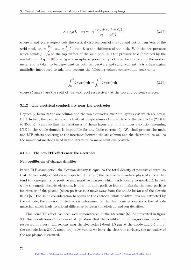
3. Numerical and experimental study of arc and weld pool couplings
λ+ ρg(L+ ψ) = −γ rψrr + ψr(1 + ψ2r )
r(1 + ψ2r )
32
(3.15)
where ϕ and ψ are respectively the vertical displacement of the top and bottom surfaces of the
weld pool. ϕr =∂ϕ
∂r, ϕrr =
∂2ϕ
∂r2, etc. L is the thickness of the disk, Pa is the arc pressure
which equals p− p0 on the top surface of the weld pool. p is the pressure field (obtained by the
resolution of Eq. 3.10) and p0 is atmospheric pressure. γ is the surface tension of the molten
metal and is taken to be dependent on both temperature and sulfur content. λ is a Lagrangian
multiplier introduced to take into account the following volume conservation constraint:
∫ rt
02πϕ(r)rdr =
∫ rb
02πψ(r)rdr (3.16)
where rt and rb are the radii of the weld pool respectively at the top and bottom surfaces.
3.1.2 The electrical conductivity near the electrodes
Physically, between the arc column and the two electrodes, two thin layers exist which are not in
LTE. In fact, the electrical conductivity at temperatures of the surface of the electrodes (2000 K
to 3500 K) is zero so that the resistances of theses layers are infinite. Thus a solution assuming
LTE in the whole domain is impossible for any finite current [6]. We shall present the main
non-LTE effects occurring at the interfaces between the arc column and the electrodes, as well as
the numerical methods used in the literature to make solutions possible.
3.1.2.1 The non-LTE effects near the electrodes
Non-equilibrium of charges densities
In the LTE assumption, the electron density is equal to the total density of positive charges, so
that the neutrality condition is respected. However, the electrodes introduce physical effects that
tend to non-equality of positive and negative charges, which leads locally to non-LTE. In fact,
while the anode absorbs electrons, it does not emit positive ions to maintain the local positive
ion density of the plasma (when positive ions move away from the anode because of the electric
field) [6]. The same consideration happens at the cathode; while positive ions are attracted by
the cathode, the emission of electrons is determined by the thermionic properties of the cathode
material, which leads to a local difference between the electron and ion densities.
This non-LTE effect has been well demonstrated in the literature [6]. As presented in figure
3.1, the calculations of Tanaka et al. [6] show that the equilibrium of charges densities is not
respected in a very thin regions near the electrodes (about 1.5 µm at the anode and 0.5 µm at
the cathode for a 200 A argon arc); however, as we leave the electrode surfaces, the neutrality of
the arc-plasma is ensured.
76
PhD Thesis: ”Multiphysics modelling and numerical simulation of GTA weld pools” - Abderrazak Traidia - 2011

3.1. Development of the mathematical model
Non-equilibrium of electron and ion temperatures
It is generally assumed, that in the arc-plasma column, collisional processes between particles
dominate over other physical processes, such as applied forces, diffusion or radiation. This leads
to averaging out of the temperature, and thus electron and ion temperatures are almost the
same. However, near the electrodes, electron temperature may differ significantly from heavy
particle temperature. In fact the heavy particle temperature is close to the electrode material
temperature (2000 K-3500 K), whereas the electrons temperature is much higher in order to
ensure the current conduction between the plasma and electrodes. To take into account this
non-LTE effect near the electrodes, one must develop a twin temperature model: electrons and
ions. The development of such a model introduces complex phenomena that lead to a lot of
numerical difficulties. This explains why such a model is not used in arc welding simulations.
Figure 3.1: Calculated electron and positive ion densities near the anode for a 200 A arc [6].
Non-equilibrium of charge densities near the anode surface.
However, the literature review shows that several methods have been developed to deal with
these non-LTE effects near the electrodes. A brief description of each method is given below.
3.1.2.2 The ambipolar diffusion method
The first method, developed by Sansonnens et al. [32], and used by Lowke, Tanaka and their
co-workers in [6, 17, 15, 46, 53], consists in taking into account the ambipolar diffusion effect
near the electrodes. In fact, instead of the usual current density representation as only dependent
on the electric field by the Ohm’s law (−→j = σ
−→E ), they also include a term accounting for the
electron diffusion current as follows:
~j = σ ~E + eDe∇ne (3.17)
where De is the electron-diffusion coefficient, e is the elementary charge and ne the electron-
number density which is governed by an additional conservation equation of electron density as
PhD Thesis: ”Multiphysics modelling and numerical simulation of GTA weld pools” - Abderrazak Traidia - 2011
77

3. Numerical and experimental study of arc and weld pool couplings
follows:
∇ · (Da∇ · ne) + S − γen2e = 0 (3.18)
where Da is the ambipolar diffusion coefficient, S = γen2eq is the source function representing ther-
mal ionisation, neq is the local equilibrium electron density and γe is the two-body recombination
coefficient. Da is usually approximated by:
Da =2De/µe
1/µe + 1/µ+(3.19)
where µe and µ+ are respectively the electron and ion mobilities.
The resolution of equation 3.18 permits calculation of the electron density field ne, and then
the computation of the diffusion current eDe∇ne appearing in equation 3.17.
While the electric current σ ~E is zero near the electrodes due to the electrical conductivity
that drops in theses regions, the additional diffusion term eDe∇ne becomes predominant and
ensures the current flow to the electrodes.
3.1.2.3 The ’LTE-diffusion’ approximation method
The second method is entitled the ’LTE-diffusion’ approximation, and was suggested by Lowke et
al. in [50]. Under this approximation, local LTE is assumed in the whole plasma domain, with a
particular mesh size near the electrodes to overcome the problem that the equilibrium electrical
conductivity near the electrodes is almost zero. In fact, taking a relatively large mesh size near
the electrodes leads to averaging out of the temperature in the anodic and cathodic zones to
about 7000 K, and then the electrical conductivity becomes non-zero. According to Lowke et al.
[50], this method gives very close results to the ambipolar diffusion method. The length of the
mesh elements near the electrodes must equal the diffusion length; i.e., the length for which the
diffusion current is negligible. Lowke et al. [50] suggested a mesh size of about 1.10−4 m at the
cathode and 4.10−4 m at the anode. This method was recently used by Brochard [1], and the
computed results were in good agreement with the literature.
3.1.2.4 The conductive layers method
The latter method, which is used in this work, assumes the anodic and cathodic zones to be an
ohmic conductor, which ensures the transition between the plasma column and the electrodes. In
order to achieve this, two thin adjacent layers respectively to the anode and to the cathode are
considered; within these layers we will consider the electrical conductivity of the corresponding
electrode, but the dynamic viscosity, thermal conductivity and specific heat of the plasma gas.
The thickness of these layers is about 1× 10⁻⁴ m which is the length of the non-LTE zone near
the electrodes. This method was suggested by Lago et al. [54] and Gonzalez et al. [56] and
was applied for the treatment of the anodic zone. The numerical results obtained by Lago et al.
[54] were compared with experimental results from the literature, and show a good agreement.
Moreover, according to Lago et al. [54], reducing the size of the conductive layer does not
78
PhD Thesis: ”Multiphysics modelling and numerical simulation of GTA weld pools” - Abderrazak Traidia - 2011

3.1. Development of the mathematical model
affect the anodic heat flux, however, some modifications appear when increasing the size of the
conductive layer to 5× 10⁻⁴ m.
The conductive layers method has been used by Lago et al. [54] only for the treatment of the
anodic region, it will be extended in this work also for the cathodic region.
3.1.3 The heat transfer at the arc-electrodes interfaces
3.1.3.1 The arc/anode interface
Based on the Tanaka et al. [6] approach, we consider the following energy balance at the interface
between the arc-plasma and the anode4:
qanode,input = qplasma,output + qelectrons,condensation − qradiation (3.20)
The above equation means that the total input heat flux at the anode is the sum of the conduction
from the plasma qplasma,output and the heating by electrons condensation qelectrons,condensation =
|~j · ~n|φa (energy received by the anode from the incoming electrons, which is the product of
the normal current density |~j · ~n| by an equivalent anode work function φa), decreased by the
radiations losses from the anode qradiation = εσBT4 (ε is the anode emissivity, T is temperature
and σB the Stefan-Boltzmann constant).
Most of the available models consider the equivalent anode work function φa to be the sum of
the anode work function φA and the anode fall voltage VA; φa = φA + VA. However, Tanaka et al.
[6] does not account for the anode-fall heating, and consider φa = φA. According to Tanaka et al.
[6], accounting for the anode-fall heating (|~j · ~n| · VA) would overestimate the energy flux into the
anode, and they argued that the anode-fall heating is already included in the term (|~j · ~n| · φa).Equation 3.20 can be formulated as follows [6]:
~qa · (−~n) = ~qpl · (−~n) + |~j · ~n|φa − εσBT 4 (3.21)
where ~qa = −ka∇Ta, ~qpl = −kpl∇Tpl, ka is the anode thermal conductivity, kpl is the plasma
thermal conductivity and Ta and Tpl represent the temperature field respectively in the anode
and plasma domains. ~n is a vector normal to the electrodes surfaces and directed toward the
plasma domain, as shown in figure 3.2.
Additionally at the anode, one must take the total shear stress ~τ at the top surface of the
weld pool is the sum of the arc drag force and the Marangoni force. Considering the assumption
of a flat free surface, this can be expressed by the following relation:
τanode = τarc + fL∂γ
∂T
∂T
∂r(3.22)
τanode =
([−paI + µa(∇~va + (∇~va)t
]· ~n)· ~s
τarc =([−pplI + µpl(∇~vpl + (∇~vpl)t
]· ~n)· ~s
4The heating of the anode by radiation from the arc plasma is neglected. This assumption is also considered by
Tanaka et al.[6]. Indeed, Ushio et al. [68] found the contribution of the radiative heat flux to the anode to be less
than 5% of the total heat input.
PhD Thesis: ”Multiphysics modelling and numerical simulation of GTA weld pools” - Abderrazak Traidia - 2011
79

3. Numerical and experimental study of arc and weld pool couplings
where, τanode and τarc are respectively the shear stress at the anode surface and the arc drag
force, ~s is a local tangent vector to the top free surface (here ~s = ~r) and∂γ
∂Tis the surface
tension gradient, which is taken as dependent on both temperature and sulfur content using
the Sahoo et al. relationship [19]. pa and ppl are the pressure fields respectively in the anode
and plasma domains. Similarly, ~va and ~vpl are the velocity fields respectively in the anode and
plasma domains.
n
n
anode
plasma
cathode
Figure 3.2: Definition of the normal vectors used in the model.
3.1.3.2 The arc/cathode interface
Similarly to the anode region, the following energy balance is considered at the interface between
the arc-plasma and the cathode [6]:
qcathode,input = qplasma,output + qions − qthermionic − qradiation (3.23)
The above equation means that the total input heat flux at the cathode is the sum of the
conduction from the plasma qplasma,output and the ions heating qions = jiVi (energy received by
the cathode from the collected ions, which is the product of the ion current ji by the the gas
ionisation potential Vi), decreased by the radiations losses from the cathode qradiation = εσBT4,
and by the thermionic cooling qthermionic = jeφc (energy required to emit electrons from the
cathode, which is the product of the electrons current je by the cathode work function φc).
Equation 3.23 can be formulated as follows [6]:
~qc · (−~n) = ~qpl · (−~n) + jiVi − jeφc − εσBT 4 (3.24)
where ~qc = −kc∇Tc, kc is the cathode thermal conductivity, kpl is the plasma thermal conductivity
and Tc and Tpl represent the temperature field respectively in the cathode and plasma domains.
~n is a vector normal to the cathode surface, and directed toward the plasma domain, as shown
in figure 3.2.
80
PhD Thesis: ”Multiphysics modelling and numerical simulation of GTA weld pools” - Abderrazak Traidia - 2011

3.1. Development of the mathematical model
For the thermionic emission at the cathode, we use the method developed by Lowke et al.
[69]; the electron current density je cannot exceed the Richardson current density jr [46]:
jr = ArT2exp
(−eφekBT
)(3.25)
where Ar is the Richardson’s constant, e the elementary charge, φe is the cathode effective work
function and kB is the Boltzmann constant. The electron and ion currents je and ji are then
deduced from the following expressions:
je =
jr if (|~j · ~n| − jr) > 0
|~j · ~n| if (|~j · ~n| − jr) ≤ 0(3.26)
ji = |~j · ~n| − je (3.27)
3.1.4 Accounting for the gas flow rate
cath
od
e
no
zzle
cR
nR
gas velocity field
Figure 3.3: Schematic representation of the gas inflow.
The gas flow rate is taken into account by imposing the value of the axial velocity field between
the welding electrode and the gas nozzle (see figure 3.3). Along this inlet boundary, the radial
gas velocity is assumed to be zero, however, the axial velocity is determined from the pipe flow
equation as follows:
~v · (−~n) = Ugas(r) =2Qmρπ
[R2n − r2 + (R2
n −R2c)
ln(r/Rn)
ln(Rn/Rc)
][R4n −R4
c +(R2
n −R2c)
2
ln(Rn/Rc)
] (3.28)
where Qm = ρQv is mass flow rate of argon shielding gas and Qv is the volume flow rate of gas.
Rn is the nozzle internal radius and Rc is the cathode radius.
PhD Thesis: ”Multiphysics modelling and numerical simulation of GTA weld pools” - Abderrazak Traidia - 2011
81

3. Numerical and experimental study of arc and weld pool couplings
3.1.5 Summary of governing equations
The governing equations, and the boundary conditions along the electrode surfaces are summarized
as follows:
In the whole domain: cathode, arc-plasma and anode
∇ ·
(σ∇V + σ
∂−→A
∂t
)= 0
σ∂−→A
∂t+
1
µ0∇×
(∇×
−→A)
+ σ∇V = ~0
ρCeqp
(∂T
∂t+ ~v · ∇T
)= ∇ · (k∇T ) + Sv
(3.29)
In the arc-plasma and anode domains
∇ · ~v = 0
ρ
(∂~v
∂t+ ~v · ∇~v
)= −∇p+∇ ·
[µ(∇~v +t ∇~v)
]+−→j ×−→B + ρ0
−→g − wpρ0β(T − Tref )−→g
(3.30)
At the free surfaces of the weld poolPa − λ− ρgϕ = −γ rϕrr + ϕr(1 + ϕ2
r)
r(1 + ϕ2r)
32
λ+ ρg(L+ ψ) = −γ rψrr + ψr(1 + ψ2r )
r(1 + ψ2r )
32
(3.31)
Along the plasma/anode interface[(−ka∇Ta)− (−kpl∇Tpl)] · (−~n) = |~j · ~na|φa − εσBT 4
τanode = τarc + fL∂γ
∂T
∂T
∂r~v · ~n = 0
(3.32)
Along the plasma/cathode interface[(−kc∇Tc)− (−kpl∇Tpl)] · (−~n) = jiVi − jeφc − εσBT 4
~v = ~0(3.33)
3.1.6 Transport properties of constitutive materials
Before presenting the results, we shall describe the transport properties of the materials used in
our calculations.
The cathode
In this work, we consider a pure tungsten cathode. The electrical and thermal conductivities of
pure tungsten as a function of temperature are taken from the recent work of Brochard [1], and
are shown in figure 3.4. The other constant properties used for the cathode are shown in table
3.1.
82
PhD Thesis: ”Multiphysics modelling and numerical simulation of GTA weld pools” - Abderrazak Traidia - 2011

3.1. Development of the mathematical model
The anode
Two kinds of materials will be considered for the anode; an AISI 304 stainless steel anode (for
the formation of a weld pool), and a water cooled copper anode (to avoid the formation of the
weld pool). The thermophysical properties of these materials are shown in figures 3.7 and 3.5.
The other constant properties used for the anode are presented in table 3.1.
The shielding gas
The shielding gas is assumed to be pure argon at atmospheric pressure. Using the Boulos et
al. tabulated values given in the literature [70], we present in figure 3.6 the evolution of the
transport properties of argon (density, specific heat, dynamic viscosity, thermal conductivity and
electrical conductivity) as function of temperature. Concerning the variation with temperature
of the net emission coefficient of argon εN , we use the same values as Lago et al. [54]. The other
constant properties used for argon are shown in table 3.1.
Figure 3.4: Thermal and electrical conductivities of pure tungsten [1].
Figure 3.5: Thermal and electrical conductivities of pure copper [1].
PhD Thesis: ”Multiphysics modelling and numerical simulation of GTA weld pools” - Abderrazak Traidia - 2011
83

3. Numerical and experimental study of arc and weld pool couplings
Symbol Nomenclature Value
φc Cathode work function 4.52 V [46]
φe Effective work function 2.63 V [46]
Ar Richardson’s constant 3×10⁴ A m−2 K−2 [46]
304 ss anode
Tl Liquidus temperature 1723 K [20]
Ts Solidus temperature 1673 K
Tref Reference temperature 1723 K
β Thermal expansion coefficient 10−4 K−1 [20]
µ Dynamic viscosity of liquid phase 0.05 kg m−1 s−1 [20]
Lf Latent heat of fusion 2.47 ×10⁵ J kg−1 [21]
ρ0 Reference density 6350 kg m−3
Aγ Constant in surface tension gradient 4.3×10⁻⁴ N m−1 K.1 [19]
Rg Gas constant 8314.3 J kmol−1 K−1 [19]
Γs Surface excess at saturation 1.3×10⁻⁸ kmol m−2 [19]
γm Surface tension at pure metal 1.943 N m−1 [19]
k1 Entropy factor 3.18×10⁻³ ([19])
φa Anode work function (without fall voltage) 4.65 V [46]
φa Anode work function (with fall voltage) 6.76 [25]
ε Anode emissivity 0.9 [20]
σ Electrical conductivity 7.7×10⁵ Ω−1 m−1 [1]
Copper anode
φa Anode work function 4.65 V [46]
ε Anode emissivity 0.9 [20]
Argon gas
Vi Ionization potential 15.68 V [46]
Table 3.1: Material properties of the cathode, the shielding gas and two different anode materials,
used in our calculations
84
PhD Thesis: ”Multiphysics modelling and numerical simulation of GTA weld pools” - Abderrazak Traidia - 2011

3.1. Development of the mathematical model
Figure 3.6: Transport properties of pure argon as function of temperature [70].
PhD Thesis: ”Multiphysics modelling and numerical simulation of GTA weld pools” - Abderrazak Traidia - 2011
85

3. Numerical and experimental study of arc and weld pool couplings
Figure 3.7: Thermal conductivity [43], density [1] and specific heat [1] of AISI 304 stainless steel.
3.2 Comparison of the results with literature
In this section we compare our numerical results with those of some models available in the
literature.
3.2.1 Comparison with Hsu study
The Hsu et al. configuration [26]
J
Figure 3.8: Geometrical configuration used by Hsu et al. [26].
86
PhD Thesis: ”Multiphysics modelling and numerical simulation of GTA weld pools” - Abderrazak Traidia - 2011

3.2. Comparison of the results with literature
Using spectroscopic emission measurements, Hsu et al. [26] determined the experimental tem-
perature field in an argon arc-plasma. Also, he proposed a simplified model of the arc-plasma
region, and the numerical results were in good agreement with his experimental measurements.
The configuration studied by Hsu et al. [26] is shown in figure 3.8. In this study they
use a thoriated tungsten cathode, a copper anode and argon as a shielding gas. The welding
current is fixed to 200 A, a 60 electrode-tip angle is considered, and the inter-electrodes distance
(arc-length) is set to 10 mm. They consider only the arc-plasma domain in their calculations, and
the main boundary conditions used are as follows (the boundary labels correspond to figure 3.8):
• Along the cathode surface AF: T = 3000 K and ~v = ~0.
• Along the anode surface BC: T = Texp (obtained experimentally, but not specified in [26]),
~v = ~0, and V=0.
• Along the top and side boundaries EF and EC: T = 1000 K and ~v · ~n = 0.
• Along the internal boundary AJ: jz = j0, where j0 is chosen in arbitrary exponential
distribution and must verify the conservation condition:
∫ J
Ajzdr = Itotal = 200 A. This
latter boundary condition is very severe, since the current density (and thus thermal and
velocity fields) in the arc-plasma are highly dependent on j0.
30°
anode
Plasma
cathode
Electrodetruncature
A
DE
J
C
IH
B
F
15
510
3
Figure 3.9: Geometry used is our model for comparison with Hsu et al. [26], dimensions in mm.
PhD Thesis: ”Multiphysics modelling and numerical simulation of GTA weld pools” - Abderrazak Traidia - 2011
87

3. Numerical and experimental study of arc and weld pool couplings
FE FA EA ED DC
T T = 1000 K ~q · ~n = 0 Eq. 3.24 T = 1000 K T = 1000 K
(u, v, p) - - ~v = ~0 p = p0 p = p0
~n · τ · ~n = 0 ~n · τ · ~n = 0
(V, ~A) ~j · ~n = IπR2
c
~j · ~n = 0 [[(~j · ~n)]] = 0 ~j · ~n = 0 ~j · ~n = 0
~B = ~0 ~A× ~n = ~0 ~A× ~n = ~0
CI IH HB BC BA
T T = 1000 K T = 1000 K ~q · ~n = 0 Eq. 3.21 ~q · ~n = 0
(u, v, p) - - - ~v = ~0 ~v · ~n = 0
(V, ~A) ~j · ~n = 0 V = 0 ~j · ~n = 0 [[(~j · ~n)]] = 0 ~j · ~n = 0~A× ~n = ~0 ~A× ~n = ~0 ~B = ~0 ~B = ~0
Table 3.2: Boundary conditions used for the Hsu et al. [26] configuration
To compare our results with those of Hsu et al. [26], we will use the geometrical configuration
used by Lago et al. [54] (also used more recently by Brochard [1]). In this configuration, presented
in figure 3.9, instead of computing the governing equations only in the arc-plasma domain (as
done in the Hsu et al. [26] model), the anode and cathode domains are also included in the
computational domain as follows; the electromagnetic problem is computed in the three domains,
the thermal field is computed in the arc-plasma and anode domains (with a water-cooled copper
anode, to avoid the formation of the weld pool), and the fluid flow is computed only in the
arc-plasma domain. Lago et al. [54] used a set of boundary conditions (including the critical
boundary condition on AJ) to reproduce the same configuration as Hsu et al. [26] model. The
boundary conditions used in our calculations are presented in table 3.2, and are similar to those
used by Brochard [1].
Results
Figure 3.10 compares our predicted arc-plasma temperature contours (right) with the experimental
measurements of Hsu et al. [26] (left). In both cases, we observe that the arc-plasma has the
typical ’bell-shape’ characteristic of argon arcs, and temperature varies from room temperature
up to 21 000 K near the cathode tip. The comparison between the two cases, shows that our
numerical results are in a good agreement with the experimental measurements, at least up to
17 000 K. The small gaps observed, can be explained by two factors; first, the errors linked to
experimental measurements increase at high temperatures, but also to the value taken for the
electrode truncation, which is not specified in [26] (in fact, an arbitrary value of 0.3 mm was
considered in our model, which could have some consequences on the computed results, this
factor will be discussed later).
Figure 3.11 presents the evolution of axial velocity in the arc column along the axis of of
discharge. Our results are compared with those obtained by the model of Hsu et al. [26]. For
both cases, we observe that the maximum jet velocity occurs a few millimetres from the cathode
tip, where the maximum Lorentz forces are located. Moreover, the agreement between the two
88
PhD Thesis: ”Multiphysics modelling and numerical simulation of GTA weld pools” - Abderrazak Traidia - 2011

3.2. Comparison of the results with literature
calculations is excellent, especially near the cathode area.
+
+
+
+
+
Figure 3.10: Our calculated temperature contours (right) compared with the experimental
measurements of Hsu et al. [26] (left).
Figure 3.11: Comparison of axial velocity of the arc-plasma jet along the arc axis.
Previously, we mentioned that both Hsu et al. [26] and Lago et al. [54] imposed directly the
evolution of the normal current density on the boundary AJ. This is of high importance, since
the computed results are dependent on the arbitrary evolution chosen for the current density.
Recently, Brochard [1] compared the numerical results of his model with the evolution of the
current density on AJ chosen by Hsu et al.; the comparison showed clear differences in both
shape and maximum values reached.
PhD Thesis: ”Multiphysics modelling and numerical simulation of GTA weld pools” - Abderrazak Traidia - 2011
89

3. Numerical and experimental study of arc and weld pool couplings
Figure 3.12: Radial evolution of the current density along the boundary (AJ): comparison of our
model with Hsu et al. [26] and Brochard [1].
Figure 3.12 shows the evolution of our computed normal current density on the boundary
AJ, also shown is the evolution obtained by Brochard [1], as well as, the arbitrary distribution
imposed by Hsu et al. [26]. As expected, the gap between our calculations and the analytical
evolution used by Hsu et al. [26] is quite important. Interestingly, we notice that in both, solution
of Brochard [1], and in our computed results, there is a drop of the current density near the
cathode tip, whereas it is not the case for Hsu et al. [26] results. This discrepancy is due to the
different values used for the cathode-tip truncations. In fact, as this value was not given by Hsu
et al. [26], we fixed the truncation to 0.3 mm, which seems to be larger than the value used by
Brochard [1], since the drop in the current density occurs in a larger zone in our work than that
of Brochard.
3.2.2 Comparison with Tanaka calculations
The Tanaka et al. configuration [46]
Figure 3.13 shows the geometrical configuration studied by Tanaka et al. in [46]. The welding
current is 150 A, argon shielding gas is used at 15 L/min flow rate, the arc-length is set to 5
mm, the electrode-tip angle is 60 and the electrode truncation is arbitrarily set to 0.3 mm. We
will consider the case where the 10 mm thick anode is made of AISI 304 stainless steel. To be
consistent with Tanaka et al.[46] calculations, we take the same value for the anode emissivity
(ε = 0.4), the anode fall voltage is not considered and the surface tension gradient is fixed to the
constant value of 4.58×10⁻⁴ N m−1 K−1. The boundary conditions used to simulate the Tanaka
et al. configuration are presented in table 3.3.
90
PhD Thesis: ”Multiphysics modelling and numerical simulation of GTA weld pools” - Abderrazak Traidia - 2011
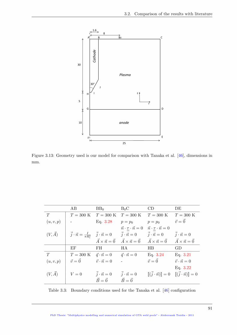
3.2. Comparison of the results with literature
A B B0 C
D
EF
G
H I
J
5
30
10
25
1.68
30°
Plasma
Cathode
r
z
anode
Figure 3.13: Geometry used is our model for comparison with Tanaka et al. [46], dimensions in
mm.
AB BB0 B0C CD DE
T T = 300 K T = 300 K T = 300 K T = 300 K T = 300 K
(u, v, p) - Eq. 3.28 p = p0 p = p0 ~v = ~0
~n · τ · ~n = 0 ~n · τ · ~n = 0
(V, ~A) ~j · ~n = IπR2
c
~j · ~n = 0 ~j · ~n = 0 ~j · ~n = 0 ~j · ~n = 0
~A× ~n = ~0 ~A× ~n = ~0 ~A× ~n = ~0 ~A× ~n = ~0
EF FH HA HB GD
T T = 300 K ~q · ~n = 0 ~q · ~n = 0 Eq. 3.24 Eq. 3.21
(u, v, p) ~v = ~0 ~v · ~n = 0 - ~v = ~0 ~v · ~n = 0
Eq. 3.22
(V, ~A) V = 0 ~j · ~n = 0 ~j · ~n = 0 [[(~j · ~n)]] = 0 [[(~j · ~n)]] = 0~B = ~0 ~B = ~0
Table 3.3: Boundary conditions used for the Tanaka et al. [46] configuration
PhD Thesis: ”Multiphysics modelling and numerical simulation of GTA weld pools” - Abderrazak Traidia - 2011
91

3. Numerical and experimental study of arc and weld pool couplings
Figure 3.14: Comparison of radial evolution of heat flux and current density at the anode for
I=150 A.
The computed radial evolution of the heat flux and current density at the top surface of the
weld pool are presented in figure 3.14. Our numerical results are compared with those obtained
by Tanaka et al. in [46]. The two studies show that the radial evolution of the current density
and heat flux at the top surface are close to a Gaussian-shape distribution, which goes with the
analytical expressions usually used in the weld pool models (see chapter 2).
However, some observations shall be discussed: first, we observe that for our model, the
heat flux is higher at small radii than the Tanaka et al. results. This can be explained by both,
the difference in the physical properties used for the AISI 304 stainless steel anode, and the
differences between the two models in the treatment of the anodic region. In fact, as the Tanaka
et al. model consider the non-LTE effects near the anode region (by adding the diffusion current),
the conductive area near the anode surface through which current flows is better estimated. This
leads to a better estimation of the electron condensation flux transmitted to the anode, and thus
to the global input heat flux at the top surface.
Moreover, analysing the current density distribution of Tanaka et al. [46], we clearly observe
a decrease near the anode axis, which is not the case for our calculations. This decrease has
not been reported in most of the published papers dealing with arc-plasma modelling. Recently,
Lowke et al. [50] explained that this off-centre maximum in the current density curve occurs
because of the diffusion current, that becomes predominant near the anode center compared to
the electric current. Figure 3.15 shows a comparison of calculated current densities at a copper
anode for a 200 A arc, obtained by Lowke et al. [50]. The results assuming the ’LTE-diffusion
approximation’ near the electrodes (which is close to the method used in this study) are compared
with those accounting for the diffusion current (noted ’full diffusion’). As seen in this figure, the
simulation that does not account for the diffusion current does not present any decrease near
the anode center, which goes with our numerical results presented in figure 3.14. However, an
off-center maximum clearly appears on the simulation accounting for the diffusion current, and
seems to be in a good agreement with the experimental results, thus inducing a better estimation
of the conductive channel in the arc plasma. Regarding the results, Lowke et al. [50] concluded
92
PhD Thesis: ”Multiphysics modelling and numerical simulation of GTA weld pools” - Abderrazak Traidia - 2011

3.2. Comparison of the results with literature
that the ’LTE-diffusion approximation’ can be reasonably used (with a particular attention given
to the mesh densities near the electrodes) to get accurate results with reduced computing times.
Figure 3.15: Comparison of calculated current densities at a copper anode for a 200 A arc [50].
Designation Formula Tanaka et al. [46] Brochard [1] Model
Conduction from the arc
∫anode
~qpl · (−~n)dS 373 845.8 548.1
Electrons condensation
∫anode
|~j · ~n|φadS 697 705 698.1
Radiation losses
∫anode
εσBT4dS 30 68.7 42
Total power at the anode
∫anode
~qa · (−~n)dS 1040 1482.1 1204.2
Table 3.4: Comparison of power terms at the anode for a 150 A argon arc (values given in W).
Table 3.4 gives the power balance at the anode for the previously studied Tanaka et al.
[46] configuration. Our results are compared with both, Tanaka et al. results and Brochard
[1] results. As seen, the agreement between the different simulations is quite satisfying. The
discrepancy between the different values is mainly associated with the different values taken for
the materials properties, and to the different methods used for the treatment of the electrode
regions. Indeed, Tanaka et al. [46] uses the ’full-diffusion method’ (which explains the lower value
obtained for total heat transferred to the workpiece), Brochard [1] made use of the ’LTE-diffusion
PhD Thesis: ”Multiphysics modelling and numerical simulation of GTA weld pools” - Abderrazak Traidia - 2011
93

3. Numerical and experimental study of arc and weld pool couplings
approximation’ method, whereas in our model the ’conductive layers method’ is used.
Figure 3.16 shows the computed surface temperature of the tungsten cathode compared with
the experimental values of Zhou and Heberlein [71]. Is is also seen, that the predicted temperature
is in good agreement with experiment. The maximum value of temperature is reached at the
cathode tip, and it is about 3500 K, which is in agreement with what is commonly reported in
the literature [71].
Figure 3.16: Theoretical surface temperature of the cathode for a 150 A argon arc and 5 mm
arc-length, compared with experimental values of Zhou and Heberlein [71].
3.3 Application I: study of pulsed current GTA welding
This section is devoted to the study of pulsed current GTAW using our coupled arc/weld-
pool model. As the welding current is varying with time, the developed model is used in its
time-dependent formalism.
3.3.1 Computational domain and boundary conditions
3.3.1.1 Materials properties and mesh densities
The calculation domain used in this section is shown in figure 3.17. The geometry includes a
tungsten cathode with a 60 angle tip and 15 mm length. The arc-plasma domain is pure argon,
and the anode is an AISI 304 stainless steel disk with a 20 mm radius and a variable thickness
named h. The inter-electrode distance is fixed to 3 mm.
In order to reduce computing time, the anode domain is made of two subdomains with
different mesh densities in each domain. The mesh size densities are as follows; 2.5×10⁻⁴ m in
the plasma and weld pool domains, 1×10⁻⁴ m in the cathode domain, and 8×10⁻⁵ m at the top
surface of the weld pool, where high thermal gradients occur.
94
PhD Thesis: ”Multiphysics modelling and numerical simulation of GTA weld pools” - Abderrazak Traidia - 2011

3.3. Application I: study of pulsed current GTA welding
The thermo-physical properties of argon, and tungsten are temperature-dependent and were
previously shown in figures 3.6 and 3.4. The constant parameters are given in table 3.1. The
numerical model is applied to AISI 304 stainless steel with 290 ppm sulfur content (as = 0.029
wt %). Contrary to chapter 1, here the thermo-physical properties of AISI 304 are temperature-
dependent and shown previously in figure 3.7, and the anode fall voltage is taken into account in
the value of the equivalent anode work function (φa = 6.76 V).
In this section, the standard heat of adsorption ∆H0 of stainless steel is fixed to the reference
value of -1.66×10⁸ J kmol−1 given by Sahoo et al. [19], rather than the value of -1.88×10⁸ J
kmol−1 given by Zacharia et al. [10] (since here, the reference value is found to give a better
agreement with experiments).
3.3.1.2 Boundary conditions
Table 3.5 lists all the boundary conditions used in this section. Some pertinent points are outlined
below:
Regarding the thermal conditions, the temperature along the external boundaries ABC and
CD is set to the ambient temperature T0 = 300 K, one must be careful to take a long enough
cathode length, in order to be sure that the temperature along the previous boundaries is close
to the ambient temperature. Along the external anode boundaries DE and EF0F the convection
heat transfer is considered by imposing :
~q · ~n = ha(T − T0) (3.34)
where ha is the anode convection coefficient (here fixed to 15 W m−2 K−1). This boundary
condition is more realistic than the usually fixed temperatures on those boundaries used in
the literature (which could have an impact on the computed anodic heat flux), it also makes
possible the full penetration of the weld pool. The normal heat flux discontinuities between the
arc-plasma and the electrodes are considered using equations 3.21 and 3.24.
Regarding the fluid flow conditions, the axial velocity along the inlet gas boundary BB0 is
determined from the pipe flow equation 3.28. Along the top surface of the weld pool, a slip
condition is considered ~v · ~n = 0, combined with the fact that the total shear stress ~τ is the sum
of the arc drag force and the Marangoni force, as expressed in equation 3.22. Along the bottom
surface of the disk, a full penetration of the weld pool may occur, and then it is necessary to
take into account the Marangoni condition (without arc drag force) as follows:
τbottom = fL∂γ
∂T
∂T
∂r(3.35)
Finally, for the electromagnetism conditions, a uniform current density is assumed at the
cathode top surface AB: ~j · ~n = j0 =I(t)
πR2c
, where Rc is electrode radius. The lateral and bottom
surfaces DEF are assumed to be earthed: V = 0.
PhD Thesis: ”Multiphysics modelling and numerical simulation of GTA weld pools” - Abderrazak Traidia - 2011
95

3. Numerical and experimental study of arc and weld pool couplings
A B B0 C
D
EF0F
G G0
H I
J
3
20
h
20
1.68
30°
Plasma
Anode
Cathode
Figure 3.17: Geometry used for pulsed current calculations. Dimensions in mm.
AB BB0 B0C CD DE
T T = 300 K T = 300 K T = 300 K T = 300K Eq. 3.34
(u, v, p) - Eq. 3.28 p = p0 p = p0 ~v = ~0
~n · τ · ~n = 0 ~n · τ · ~n = 0
(V, ~A) ~j · ~n = I(t)πR2
c
~j · ~n = 0 ~j · ~n = 0 ~j · ~n = 0 ~j · ~n = 0
~A× ~n = ~0 ~A× ~n = ~0 ~A× ~n = ~0 ~A× ~n = ~0
EF0F FH HA HB GG0D
T Eq. 3.34 ~q · ~n = 0 ~q · ~n = 0 Eq. 3.24 Eq. 3.21
(u, v, p) ~v · ~n = 0 ~v · ~n = 0 - ~v = ~0 ~v · ~n = 0
Eq. 3.35 Eq. 3.22
(V, ~A) V = 0 ~j · ~n = 0 ~j · ~n = 0 [[(~j · ~n)]] = 0 [[(~j · ~n)]] = 0~B = ~0 ~B = ~0
ϕ - - - - G: ∂ϕ∂r = 0
- - - - Eq. 3.16
ψ F: ∂ψ∂r = 0 - - - -
Eq. 3.16 - - - -
Table 3.5: Boundary conditions used for the study of pulsed current configuration.
96
PhD Thesis: ”Multiphysics modelling and numerical simulation of GTA weld pools” - Abderrazak Traidia - 2011

3.3. Application I: study of pulsed current GTA welding
3.3.1.3 Numerical procedure
All the equations of the problem are rewritten in a weak form and solved using the finite element
method. The computational domain is meshed using standard quadratic Lagrangian triangular
elements. The mesh density in each region has been given previously.
As the arc ignition cannot be modelled using the current approach, it is ensured numerically
by imposing a conductive channel between the two electrodes at t=0. This was also used recently
by Brochard [1] as follows:
σt=0 = 500 exp(−500r) + 1 [S/m] (3.36)
After a time step, the electric and magnetic potentials are first computed. Then the current
density, electric field and magnetic induction are deduced in the whole domain. The computed
Joule heat source is then used to calculate the temperature field. Pressure and velocity are
obtained using the previously computed thermal field and the Lorentz forces.
If the convergence criteria are not reached (absolute tolerance fixed to 10−6), the thermo-
physical properties are updated using the current temperature, and calculations will continue
until convergence. Finally the free surfaces shapes of the weld pool are computed. The whole
process is repeated at each time step until the end of welding time. The time step is 0.01 s and
computations are performed within 6 h on a 6 processor computer.
3.3.2 Results
In the present section, we will first present the results for a given pulsed welding case by studying
both arc and weld pool results. Then we will compare welding under constant current and pulsed
current considering the anodic flux and weld pool dynamics. Finally, the disk thickness will be
reduced to quantify its impact on the anodic heat flux distribution with full penetration of the
weld pool.
The operating parameters are the same for all the results presented in this section, they are
listed in table 3.6.
Symbol Nomenclature Value
Ip Peak pulse current 160 A
Ib Background current 80 A
tp Peak pulse duration 0.5 s
tb Background duration 0.5 s
Q Argon inflow rate 30 L min−1
f Pulse frequency 1 Hz
tt Total heating duration 15 s
np Number of periods 15
Table 3.6: Welding parameters used for the study of pulsed current GTAW.
PhD Thesis: ”Multiphysics modelling and numerical simulation of GTA weld pools” - Abderrazak Traidia - 2011
97

3. Numerical and experimental study of arc and weld pool couplings
3.3.2.1 Partial penetration
In this part the thickness of the plate is fixed to h = 8 mm in order to avoid the full penetration
of the weld pool. The other dimensions of the computational domain were previously introduced
and shown in figure 3.17.
Figure 3.18 shows the time evolution of the calculated solution at the end of the background
time and the peak time every five periods, which are periods 1, 5, 10 and 15. At each period
the temperature field in the arc column and the cathode domains are shown. The temperature
contours between 8000 K and 17000 K, the normalized velocity vector field and the streamlines
inside the molten weld pool are also shown to identify vortices. To make it easy to understand
only the contours for temperatures of 8000 K and above are shown, the gap between two contours
is 1000 K.
8000
8000
t=9.5 s t=10 s
Tmax=14 253 KUmax=33.6 m/s Tmax=16 690 K
Umax=116 m/s
8000
8000
t=14.5 s t=15 s
Tmax=14 253 KUmax=33.6 m/s
Tmax=16 547 KUmax=112 m/s
(a)
(b)
(c)
(d)
Figure 3.18: MHD solutions at background times (left) and peak times (right), for the periods:
(a) 1, (b) 5, (c) 10 and (d) 15.
The comparison between the background and peak times at each period shows that tempera-
ture is higher during the peak time and the arc column is wider. Moreover by considering the
temperature contours above 11000 K the arc is bell-shaped during the peak pulse duration whilst
98
PhD Thesis: ”Multiphysics modelling and numerical simulation of GTA weld pools” - Abderrazak Traidia - 2011

3.3. Application I: study of pulsed current GTA welding
not during the background duration. This is due to the electromagnetic forces that become
higher during the peak time, inducing a higher plasma jet velocity, which causes the bell-shaped
form. This qualitative result is in good agreement with the Infra-red observations (discussed
further), where the pulsed arc is bright and large during the peak time, dark and contracted
during the background time.
The maximum temperature of the tungsten cathode is found to be around 3500 K at peak
time and 3200 K at background time. In the arc-plasma domain the maximum temperature and
plasma-jet velocity are varying respectively from 14 250 K and 33 m s−1 at the background time
to 16 540 K and 118 m s−1 at the peak time. These values are highly dependent on the chemical
composition of the shielding gas composition, the welding current and the arc length. We also
note that the variations between the first peak time and the last peak time are negligible (about
1 % for the temperature and 5 % for the velocity), this is also when comparing the first and the
last background times.
A review of the literature [7] shows that, in the case of 150 A arc current (with 5 mm
arc-length), 17 000 K and 100-150 m s−1 respectively for the maximum temperature and the
plasma-jet velocity have been given elsewhere [7]. As the maximum value of plasma-jet velocity
is on the axis of symmetry, there is a discrepancy between the maximum values obtained by the
different authors. This is due to both, the singularity of the Ampere’s law at r = 0, and to the
various numerical methods that are used (finite element, finite volume, etc.).
Regarding the weld pool dynamics, we can clearly see in figure 3.18 two vortices; named A
and B. It is also seen that at each peak time the vortex B is predominant which induces an
outward fluid flow resulting in a shallow and wide weld pool. Whereas, at each background time
the vortex A is predominant inducing an inward fluid flow and resulting in a deep and narrow
weld pool.
Figure 3.19: surface tension gradient as function of temperature for a 290 ppm stainless steel
(left), and surface temperature distribution at last peak and background times (right).
This alternation (which was discussed in the previous chapter) is due to the sign change
PhD Thesis: ”Multiphysics modelling and numerical simulation of GTA weld pools” - Abderrazak Traidia - 2011
99

3. Numerical and experimental study of arc and weld pool couplings
of ∂γ/∂T . Indeed, as shown in figure 3.19 (left), the surface tension gradient is positive until
temperature reaches a critical temperature Tc = 2146 K with a maximum of 5.22×10⁻⁴ N m−1
K−1, it then becomes negative for higher temperatures and reaches a minimum of -3.15×10⁻⁴ N
m−1 K−1. Figure 3.19 (right) shows that the maximum surface temperatures during the peak
and background times are above the critical temperature Tc, which explains the existence of two
vortices in each picture; a vortex A corresponding to the region where ∂γ/∂T > 0 and a vortex B
corresponding to the region where ∂γ/∂T < 0. The region where T > Tc is larger during the
peak time which explains the domination of vortex B. Whereas during the background time the
region where T < Tc is larger which causes the predomination of vortex A.
Figure 3.20 shows the anodic heat flux and current density distributions during the transition
from the last background time (t = 14.5 s) to the last peak time (t = 15 s). During the
background time the maximum of anodic flux and current density are respectively 43 W/mm2
and 5.7 A/mm2. The transition is very fast, especially at the center of the plate where the peak
time solution is reached in approximately 15 ms; the maximum reached heat flux and current
density are respectively 56.5 W/mm2 and 6.83 A/mm2. We can also notice that, even if the
maximum value of the solution does not vary after 15 ms, the radius of the distribution continues
to increase, especially for the current density.
Figure 3.20: Radial distributions at the anode of the heat flux (left) and current density (right)
during the transition from the last background time to the peak time.
3.3.2.2 Comparison with the mean current
In engineering computations, pulsed current welding is usually approximated by the mean current
between the peak and background currents, which is constant with time. This approximation is
often used for the determination of residual stresses and distortions after welding. Here, we are
interested in the comparison between the previously obtained results (80/160 A, 1 Hz) with the
continuous mean current of 120 A. The welding conditions (geometrical configuration and total
heating time) remain the same, only the welding current is set to the constant value of 120 A.
The comparison in terms of anodic heat flux and current density between the pulsed current
100
PhD Thesis: ”Multiphysics modelling and numerical simulation of GTA weld pools” - Abderrazak Traidia - 2011

3.3. Application I: study of pulsed current GTA welding
and the corresponding mean current is shown in figure 3.21. In each case, the solution for the
continuous mean current 120 A at the end of heating (t = 15 s) and the solutions for the pulsed
current 80/160 A at the last background time (t = 14.5 s) and the last peak time (t = 15 s)
are represented. As expected, in both figures the mean current solution is located between the
background and peak times solutions. The maximum of heat flux and current density for the
continuous current, are respectively 51.3 W/mm2 and 6.4 A/mm2.
The total anodic heat power is obtained by integrating the heat flux on the top surface. As
regards the pulsed current case it is around ∼1380 W at peak time and ∼682 W at background
time, while it is around 1040 W for the continuous current at t = 15 s. This means that the
continuous current is almost energetically equivalent to the pulsed current ((1080 + 682)/2 = 1031
W).
Figure 3.21: Comparison between pulsed current welding and the corresponding mean current in
terms of anodic heat flux (left), and anodic current density (right).
Figure 3.22: Comparison between pulsed current welding and the corresponding mean current in
term of weld pool dimensions (left), and molten zone volume (right).
PhD Thesis: ”Multiphysics modelling and numerical simulation of GTA weld pools” - Abderrazak Traidia - 2011
101

3. Numerical and experimental study of arc and weld pool couplings
Figure 3.22 (left) shows the time evolution of the weld pool half-width and depth for the
continuous current 120 A and the pulsed current 80/160 A. Although the two cases are found
to be ”energetically” equivalent, it is remarkable to see that the pulsed current case produces
a deeper and wider weld pool than the continuous current case, especially for the weld depth
where the difference between the two cases is around 1 mm. Indeed, this is due to the periodic
domination of vortices A and B discussed in the previous section. This confirms the suggestion
given in the previous chapter; for a given energy level, it is more interesting to use a pulsed
current weld.
The same conclusions are available when comparing the molten weld pool volumes, as shown
in figure 3.22 (right). This leads the conclusion that not only the weld pool dimensions are larger
for the pulsed case, but also the molten zone volume (which was not obvious).
3.3.2.3 Effect of the full penetration
In this part, the thickness of the plate h is reduced from 8 mm to 4 mm to ensure the full
penetration of the weld pool. All the other process parameters remain the same as the thick
plate simulation and are listed in table 3.6.
The computed solutions are shown in figure 3.23. After calculation, the full penetration
occurs during the fifth period of heating. Figure 3.23 (left) compares the solutions at the end of
the fifth background time (t = 4.5 s) and peak time (t = 5 s); i.e., just before and just after the
full penetration. Regarding the temperature field in the arc-plasma domain, the conclusions are
the same as discussed in the partially penetrated case.
Figure 3.23: Computed solution at the fifth period of heating: MHD solution before and after
the full penetration (left), and top and bottom free surfaces shapes (right).
As regards the fluid flow inside the weld pool, we can identify in each figure the vortices A
and B which were previously analysed. In opposition to the partially penetrated case, here the
vortex B is predominant during both peak and background times; as the thickness of the plate is
102
PhD Thesis: ”Multiphysics modelling and numerical simulation of GTA weld pools” - Abderrazak Traidia - 2011

3.3. Application I: study of pulsed current GTA welding
reduced, the temperature at the top free surface is higher, which leads to have a large zone with
negative surface tension gradient, and thus increases the zone where the fluid flow is outward.
At time t = 4.5 s, we can also observe the appearance of a new vortex (named C) inducing an
inward flow, under the two main vortices A and B. As the buoyancy force and the Lorentz force
are known to create respectively outward and inward flows [18], the new vortex is necessarily the
result of the electromagnetic forces (since the fluid flow induced by vortex C is inward).
As regards the free surface deformation, figure 3.23 (right) shows the time evolution of the top
and bottom free surfaces between t = 4.5 s (end of a background time) and t = 5 s (end of a peak
time). It is seen that the top free surface is deformed under the actions of arc pressure, gravity
and surface tension. As the arc pressure is higher during the peak time than the background
time the free surface is more deformed. The maximum depression reached for the peak time
is around 0.1 mm which is very small compared to the weld pool dimensions. This is in good
agreement with the assumption that the free surface could be considered as ”flat” for the MHD
couplings. However, as the arc attaches preferentially to the higher regions, the deformation of
the free surface may cause a change in both the current density and heat flux distributions at
the anode. Currently, no model is available in the literature to deal with unified arc and weld
pool modelling considering self-consistently the free surface deformation. Efforts must be made
in this direction, to quantify the effects of the surface deformation on the transfer phenomena
between the arc and the weld pool.
As shown previously in figure 3.23 (right) the full penetration of the weld pool occurs around
t = 4.8 s, and the bottom free surface starts deforming at the end of the peak time t = 5. It is
seen that the bottom deformation increases, as the bottom weld pool width increases. As the
two free surfaces are linked by the mass conservation, the deformation of the top free surface
increases as the weld pool is penetrating. This leads to conclude that a strong coupling is needed
between the free surfaces deformations and the MHD couplings when the full penetration of the
weld pool is reached (here for t > 5 s).
As the fluid flow and heat transfer governing equations are computed on the initial geometry
(’flat’ free surface), the computed results for the fully penetrated weld pool are valid only up
to time t = 5 s. In fact, as discussed previously, beyond t = 5 s, the free surface deformation
becomes important, and a self-consistent calculation of the free surface deformation is needed.
However, we present here qualitatively in figure 3.24, the results of our model for welding times
beyond t = 5 s. The remarkable fact here, is to see that as the full penetration of the weld pool
increases, a new vortex (named D) appears on the bottom side of the plate, which is due to the
Marangoni shear stress.
This new vortex tends to pull the molten metal toward the center of the weld pool, which is due
to the positive sign of the surface tension gradient at the bottom side of the disk. It is interesting
to notice that vortex D increases with time, up to ’eliminating’ the electromagnetically-induced
vortex C. This qualitative observation leads to an interesting conclusion; the fluid flow directions
near the free surfaces (top and bottom) are always governed by the Marangoni shear stress on
PhD Thesis: ”Multiphysics modelling and numerical simulation of GTA weld pools” - Abderrazak Traidia - 2011
103

3. Numerical and experimental study of arc and weld pool couplings
both sides of the disk, however, as we leave the free surfaces, the influence of the surface tension
decreases, and the electromagnetic forces become more dominant. Additionally, for thin plates
(as is the case here), the electromagnetically-induced vortex can even be completely ’eliminated’
by the Marangoni-induced vortices.
t=5 s t=5.1 s
t=5.2 s t=5.4 s
Negative Marangoniat the top surface
Vortex (B)
Positive Marangoniat the bottom surface
Vortex (D)
Positive Marangoniat the top surface
Vortex (A)
Electromagnetic effect
Vortex (C)
Figure 3.24: Time evolution of the weld pool and normalized velocity field after time t=5 s.
Figure 3.25: Radial evolution of the anodic heat flux for the thick disk (h = 8 mm) and the thin
disk (h = 4 mm).
104
PhD Thesis: ”Multiphysics modelling and numerical simulation of GTA weld pools” - Abderrazak Traidia - 2011

3.3. Application I: study of pulsed current GTA welding
We now present the comparison between the partial and full penetration cases regarding the
anodic heat flux. figure 3.25 shows the radial evolution of the anodic heat flux for the two studied
cases at the end of the last peak and background times. As seen, the heating power transferred
to the anode seems not to be very influenced by the thickness of the plate. In fact, the maximum
difference between the curves is located at the center of the anode and equals 0.6 W/mm2. This
result was unpredictable; for a given set of operating parameters, the energy transferred to the
workpiece depends ’highly’ on the anode material and much less on its dimensions.
3.3.3 Experimental validation
In most of the available studies of arc welding, the validation of the numerical results is conducted
by comparing the computed weld shape, with the final molten zone obtained by experiments. In
this work, we propose a validation in time for the evolution of the weld pool width. To achieve
this, we used an Infra-Red (IR) camera with a macro lens to capture the images of the weld pool
during the whole welding operation.
3.3.3.1 Experimental procedure
The experimental configuration is that studied numerically during partially penetrated welding;
we considered a spot GTA weld of an AISI 304 stainless steel disk (40 mm in diameter and 8
mm in thickness), a tungsten electrode (diameter of 3.2 mm with 60 tip angle) was used with a
3 mm arc-length length, and argon was used as a shielding gas at a flow rate of 15 L/min. The
welding parameters were manually adjusted to Ip = 160 A, Ib = 80 A and f = 1 Hz. The total
heating time is 15 s.
To capture the weld pool images, we used a FLIR c© S60 IR camera equipped with a 50 microns
macro lens with 50 Hz images frequency. Although we are not interested in the determination of
the temperature field for the time being, we used an IR camera instead of a high speed camera,
because the images were too bright (strong arc illumination) when using a high speed camera,
which prevented us to clearly see the weld pool evolution. As the IR camera measures less of
the emission from the plasma (which is mainly in the ultraviolet and visible) and most of the
emission from the metal, we were less disrupted by the arc illumination.
A Matlab c© algorithm has been developed to process the images. It decomposes each image
in its RGB components, and stores the results in matrices. Then it processes the best component
(or channel) that permits to clearly identify the weld pool frontiers (here the green channel). The
weld pool width is then determined in pixels in each image, and to get the conversion in mm, the
scale is obtained using the fact that we know the real diameter of the electrode (d = 3.2 mm)
appearing in each image.
As the pulse frequency is set manually, the developed algorithm also permits the determination
of its exact value from the images processing. The real frequency is then sent to the numerical
model as an input parameter. In our experiments, the real frequency is found to be 1.04 Hz
instead of the manually set value of 1 Hz. The real pulse frequency (1.04 Hz) is used in the
PhD Thesis: ”Multiphysics modelling and numerical simulation of GTA weld pools” - Abderrazak Traidia - 2011
105
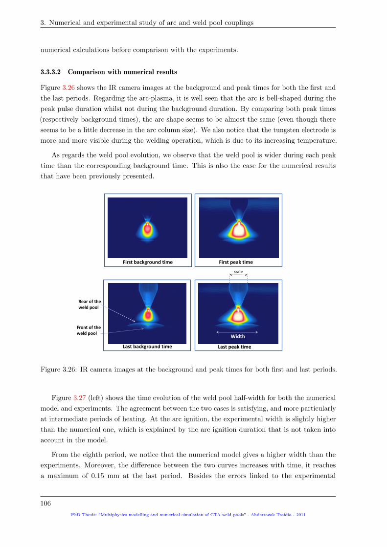
3. Numerical and experimental study of arc and weld pool couplings
numerical calculations before comparison with the experiments.
3.3.3.2 Comparison with numerical results
Figure 3.26 shows the IR camera images at the background and peak times for both the first and
the last periods. Regarding the arc-plasma, it is well seen that the arc is bell-shaped during the
peak pulse duration whilst not during the background duration. By comparing both peak times
(respectively background times), the arc shape seems to be almost the same (even though there
seems to be a little decrease in the arc column size). We also notice that the tungsten electrode is
more and more visible during the welding operation, which is due to its increasing temperature.
As regards the weld pool evolution, we observe that the weld pool is wider during each peak
time than the corresponding background time. This is also the case for the numerical results
that have been previously presented.
First background time First peak time
width
Rear of the weld pool
Front of the weld pool
Last background time Last peak time
width
scale
Width
Figure 3.26: IR camera images at the background and peak times for both first and last periods.
Figure 3.27 (left) shows the time evolution of the weld pool half-width for both the numerical
model and experiments. The agreement between the two cases is satisfying, and more particularly
at intermediate periods of heating. At the arc ignition, the experimental width is slightly higher
than the numerical one, which is explained by the arc ignition duration that is not taken into
account in the model.
From the eighth period, we notice that the numerical model gives a higher width than the
experiments. Moreover, the difference between the two curves increases with time, it reaches
a maximum of 0.15 mm at the last period. Besides the errors linked to the experimental
106
PhD Thesis: ”Multiphysics modelling and numerical simulation of GTA weld pools” - Abderrazak Traidia - 2011

3.4. Application II: influence of the shielding gas composition
measurements, we have explained this difference in the width by the accumulation of metal
vapours in the arc column. Indeed, the presence of metal vapours such as iron and chromium
(coming from the vaporization at the anode) modifies the transport properties of the plasma, in
particular it has been reported that the vapours increase the radiation emission coefficient and
the electric conductivity of the plasma [17], especially for helium arcs. This could greatly affect
the efficiency of the process which has been numerically reported to decrease from 80% to 35%
for pure helium arcs [17]. This important decrease in the efficiency of the process leads to reduce
the energy transferred to the anode, and induces a decrease in the weld pool width.
Figure 3.27 (right) shows the comparison between the macrograph of the final molten zone
and the corresponding predicted weld shape after solidification. It shows a good agreement in
terms of shape and dimensions.
Figure 3.27: Comparison between experiments and numerical predictions: time evolution of the
weld pool half width (left), and final weld shape (right).
3.4 Application II: influence of the shielding gas composition
As the electrodes rapidly oxidise in the presence of oxygen at high temperatures, they are
protected by a shielding gas that is passed through a nozzle surrounding the cathode. The
most common shielding gas is argon, which is inert and relatively inexpensive. However its
main disadvantage is that the heat source provided is diffuse and relatively low, which restricts
considerably the weld penetration. The extensive use of Gas Tungsten Arc Welding in the
manufacturing industry has lead engineers toward optimizing welding parameters to increase
productivity and improve welding quality.
3.4.1 Different methods of gas supplying
The supply of gas mixtures
An important trend introduced in the early 1970s, is the use of gas mixtures as a shielding
gas (hereafter called conventional method); argon is replaced by mixtures of argon and helium,
PhD Thesis: ”Multiphysics modelling and numerical simulation of GTA weld pools” - Abderrazak Traidia - 2011
107

3. Numerical and experimental study of arc and weld pool couplings
argon and hydrogen, or other mixtures. Each mixture has its own thermophysical properties and
produces unique arc characteristics.
The ratio of each gas in the mixture has a significant importance, it is always determined
by experimental tests and is dependent on the welding conditions, and the welded materials
(austenitic stainless steel, nonferrous materials, etc.). For this reason, over the past few years,
there has been a substantial experimental works in this direction. For example Marya et al. [72]
and Onsoien et al. [73] measured weld profiles for GTA welding of magnesium alloys (Marya et al.
[72]) and stainless steels (Onsoien et al. [73]), using argon, and mixtures of argon, helium, and
nitrogen with hydrogen. Figure 3.28 presents their experimental results showing the dependence
of the weld depth on hydrogen concentration. It is seen that the weld depth is increased by the
addition of hydrogen (H2), in particular, only a small percentage of hydrogen (as low as 1%) is
needed to increase the weld depth.
Figure 3.28: Dependence on hydrogen content of the weld depth for GTA welding using mixtures
of argon and hydrogen. Results are given for different arc currents, arc lengths and anode metals.
Taken from [17].
Tusek et al. [74] investigated experimentally the influence on the melting rate of the workpiece,
of adding hydrogen to argon in GTA welding of stainless steel, low alloy steels and aluminium
alloy. Their results are presented in figure 3.29. Again, it is found that the melting rate is
increased by the addition of any fraction of hydrogen, and the addition of only 10% of hydrogen
results in doubling the weld penetration.
Although the addition of hydrogen increases the weld penetration, it introduces serious defects
after welding (such as porosity, Hydrogen Induced Cracking (HIC), and Cold Cracking), and is
therefore used only in special cases such as welding of light-gauge stainless steel and nickel-based
alloys. In the nuclear industry, where high safety of assemblies must be ensured, one prefers
108
PhD Thesis: ”Multiphysics modelling and numerical simulation of GTA weld pools” - Abderrazak Traidia - 2011

3.4. Application II: influence of the shielding gas composition
the use of helium (He) mixed with argon (despite the high cost of helium gas). This permits to
significantly increase both the weld penetration and the welding speed.
The effects of helium addition on the heat transfer and current density at the anode have
been recently studied by Murphy et al. [17]. As shown in figure 3.30, Murphy et al. [17] showed
that the heat flux at the anode is considerably increased, and becomes more constricted by
the addition of any amount of helium to argon. Then, the weld penetration is expected to be
significantly increased. Although, Murphy et al. [17] proposed an analysis of helium addition on
the transfer phenomena between the arc and the anode, calculations were mainly done on water
cooled anode without weld pool formation.
Tanaka and Lowke [6] performed some calculations on a molten stainless steel anode, but to
reduce computing time, an arbitrary constant surface tension gradient for the Marangoni effect
was assumed. However, as previously shown in the first chapter, the Marangoni effect is the
most important driving force inside the weld pool, then, Tanaka and Lowke [6] calculations lead
to limited conclusions on the molten metal flow directions and thus on the final molten zone
dimensions. Moreover, Tanaka and Lowke [6] proposed an analysis with pure argon and pure
helium shielding gases. The effects of different argon-helium mixtures on the fluid flow directions
and the resulting weld shape remains misunderstood.
Figure 3.29: Dependence on hydrogen content of the melting rate of the workpiece for GTA
welding. Results are given for different arc currents, arc lengths and anode metals. Taken from
[17].
PhD Thesis: ”Multiphysics modelling and numerical simulation of GTA weld pools” - Abderrazak Traidia - 2011
109

3. Numerical and experimental study of arc and weld pool couplings
Figure 3.30: Radial dependence of (a) heat flux, (b) current density, (c) shear stress and (d)
arc pressure at the anode for arcs in mixtures of argon and helium. The results are for an arc
current of 150 A and an arc length of 5 mm. Taken from [17].
The alternate supply of shielding gases
Recently, Russian engineers proposed for the first time a new method of delivering shielding
gas for arc welding (originally proposed by O.M. Novikov [75] for spacecraft applications). This
method uses an equipment known as the Gas PulserTM(manufactured by the South Korean
company KR Precision Co. Ltd, and shown in figure 3.31) to deliver alternatively two pure
shielding gases (hereafter called alternate method): instead of supplying a mixed argon-helium
gas, pure argon and pure helium are alternatively supplied in the weld zone.
Two experimental studies were carried out by KR Precision Co. Ltd [76]. The effects of
alternate supply of shielding gases were studied for GMAW of aluminium and GTAW of austenitic
stainless steel. In both cases, the alternate supply of pure argon and pure helium was compared
to the use of conventional (33% argon + 67% helium). In the GMAW study, the alternate method
was found to produce a lower degree of weld porosity and deeper and broader weld shape. In the
GTAW study, the alternate method permitted an increase in the welding speed without loss of
weld penetration, and less weld distortion was found.
More recently, Kang et al. [77] investigated this new supplying method on austenitic stainless
steels, using an electromagnetic valve, as shown in figure 3.32. As seen, when the valve is located
on the left side Ar or He is supplied, while the valve is located on the center, mixture of Ar
and He is simultaneously supplied, and finally, pure Ar or pure He is supplied when the valve is
located on the right side. Kang et al. [77] found that this new technique permits to increase
the welding speed and reduces the distortions after cooling. Moreover, for a given set of welding
parameters (current, arc voltage, gas supplying frequency, etc.), the weld dimensions obtained
110
PhD Thesis: ”Multiphysics modelling and numerical simulation of GTA weld pools” - Abderrazak Traidia - 2011

3.4. Application II: influence of the shielding gas composition
when using this new technique are found to be nearly the same than those obtained by a mixture
of (33% argon + 67% helium). Consequently, Kang et al. [77] concluded that the alternate
method is cost saving compared to the conventional method of supplying gas mixtures.
Concerning the numerical simulation of alternate supply of shielding gases, the only available
numerical study was recently proposed by Kim et al. [78]. They analysed the transition of the
arc from argon to helium, but no conclusions were given on the resulting weld shapes. The
impact of alternate supply of shielding gases on the weld pool dynamics is still unknown.
Figure 3.31: Rear view of the Gas PulserTM showing the inputs and the output of the shielding
gases (left), and schematic representation of the gas pulsing switching system. Taken from [76].
Figure 3.32: Schematic diagram showing sequence alternate supply of shielding gases by electro-
magnetic valve. Taken from [77].
3.4.1.1 Objectives
Using the time-dependent unified model developed in this chapter, we intend in this section to
report on a numerical study of both the conventional method and the alternate method, in the
case where argon and helium shielding gases are used. This would permit not only investigation
of the effects of various argon-helium mixtures on the heat transfer and fluid flow in both the
arc plasma and the weld pool, but also, to analyse the arc and weld pool dynamics when the
alternate method is used.
The results of the present study are divided into two parts:
PhD Thesis: ”Multiphysics modelling and numerical simulation of GTA weld pools” - Abderrazak Traidia - 2011
111

3. Numerical and experimental study of arc and weld pool couplings
The first part analyses the conventional method: different helium-argon shielding gas mixtures
are considered, so as to study the impact of helium addition on both the transfer phenomena
between the arc plasma and the weld pool, and on the main forces that govern the weld pool
dynamics. In order to get more predictive results, the surface tension gradient is taken dependent
on both temperature and sulfur activity of the stainless steel anode. An experimental validation
on the final weld dimensions is also proposed for pure helium and pure argon arcs.
In the second part, a numerical study of the alternate method is conducted to quantify the
impact of pulsed supply of argon and helium on the weld pool time evolution, and then on the
weld shape. We also propose a comparison of the alternate method with the conventional method,
in terms of energy transferred to the workpiece and weld shape.
3.4.2 Analysis of the conventional method
In this section, an analysis of the conventional method is presented, where various mixtures of
argon and helium are used as a shielding gas. Calculations are done for an arc current of 180 A,
an arc length of 3 mm and a total heating time of 8 s. The cases of pure argon, pure helium,
and three different argon-helium mixtures are simulated to study the influence of helium mole
fraction in the mixture on the computed results. The gas inflow rate is fixed to 30 L min−1 for
all cases.
3.4.2.1 Computational domain and material properties
The computational domain is shown in figure 3.33. The geometry includes a tungsten cathode
with 60 tip-angle 20 mm length and 0.3 mm truncation. The arc plasma is either pure argon
or pure helium for the alternate method, or a mixture of argon an helium for the conventional
method. The anode is an AISI 304 stainless steel disk with 20 mm radius and 10 mm thickness,
and containing 40 ppm of sulfur. The inter-electrodes distance is fixed to 3 mm.
The material properties of the tungsten cathode and the AISI 304 stainless steel anode are
dependent on temperature, and were given previously in figures 3.6, 3.4 and table 3.1 (here
we use the value φa = 4.65 V for the anode work function). In this study, we changed the
dynamic viscosity of the molten pool to 3×10⁻² kg.m−1.s−1 (which is the value used recently
by Brochard [1]), since this value is found to give a better agreement of the computed weld
shape with the experimental results. Also, instead of considering a constant value for the anode
convection coefficient ha, we make use of the Vinokurov’s combined heat transfer coefficient
ha = 24.1× 10−4 × 0.9× T 1.61, as proposed by Goldak et al. [79] and most recently used by Bag
et al. [80]. The anode anode emissivity was set to 0.9 [81]. The standard heat of adsorption ∆H0
of the stainless steel disks, is fixed to the the value of -1.88×10⁸ J kmol−1 given by Zacharia et
al. [10].
The boundary conditions used in this chapter are the same as the studied case of pulsed
current GTAW, and were given previously in Table 3.3.
112
PhD Thesis: ”Multiphysics modelling and numerical simulation of GTA weld pools” - Abderrazak Traidia - 2011

3.4. Application II: influence of the shielding gas composition
Figure 3.33: Computational domain used for calculations. Dimensions are in mm.
The thermodynamic and transport properties of helium-argon plasmas are taken from the
recent works of Murphy et al. [17], and are shown in figure 3.34.
The net radiative emission coefficient and the density of each argon-helium mixture are
determined using a mole-fraction-weighted sum of the coefficients and densities of the component
gases as follows:
εNmixture = xArεAr + xHeεHe
ρmixture = xArρAr + xHeρHe(3.37)
where xAr and xHe are respectively the mole fractions of argon and helium in the mixed gas.
Due to the lack of experimental values, the ionization potentials of the different gases mixtures
are assumed to be that of pure argon gas (previously given).
The computational domain shown in figure 3.33 is meshed using standard Lagrangian quadratic
triangular elements. The mesh densities are as follows: he mesh size densities are as follows;
2.5×10⁻⁴ m in the plasma and weld pool domains, 1×10⁻⁴ m in the cathode domain, and 8×10⁻⁵
m at the top surface of the weld pool, where high thermal gradients occur. The time step is 0.01
s and computations are performed within 1 hour on a 6 processors computer.
PhD Thesis: ”Multiphysics modelling and numerical simulation of GTA weld pools” - Abderrazak Traidia - 2011
113

3. Numerical and experimental study of arc and weld pool couplings
Figure 3.34: Thermophysical properties of argon-helium mixtures, taken from [17]. Percentages
are mole percentages.
Concerning the finite element mesh we used the same discretization and mesh sizes as in the
previous section with pulsed current welding.
3.4.2.2 Effects on the anodic heat flux and current density
The radial evolutions of the normal heat flux and current density at the anode for each gas
mixture are shown in figure 3.35. Compared to pure argon arc, it is seen that the addition of
any fraction of helium increases the heat flux and current density at the top surface. The heat
flux density for a pure helium arc is larger on axis by a factor of 6.5. In addition, not only
the maximum values on the arc axis are increased, but also the area below the curve, which
is representative of the total energy transferred to the workpiece. This is the consequence of
two effects; the increase of thermal conductivity, and the arc constriction. Indeed, the thermal
conductivity of argon-helium mixtures increases with helium mole fraction (see figure 3.34), which
leads to an enhancement in the conductive heat flux from the plasma to the anode. Moreover, as
seen in figure 3.34, the electrical conductivity of helium arc is lower than that of argon arc, which
114
PhD Thesis: ”Multiphysics modelling and numerical simulation of GTA weld pools” - Abderrazak Traidia - 2011

3.4. Application II: influence of the shielding gas composition
leads to a reduction in the diameter of the current channel and causes the constriction of the
zone through which heat and current flow to the anode. As the arc becomes more constricted,
the maximum values of both current density and heat flux on axis increase.
Figure 3.35: Radial evolution of the anodic heat flux (left), and current density (right) for
different argon-helium mixtures. The welding current is 180 A, and the arc length is 3 mm.
It is remarkable to see that the presence of a small amount of argon (as low as 10%) in the
gas mixture reduces the heat flux on axis nearly by a factor of 2.5. This finding is also explained
by the electrical conductivity of argon-helium mixtures that is much closer to that of pure argon
than to the pure helium one (see figure 3.34). This induces the concentration of the heat flux at
higher radii for all the argon-helium mixtures, and then the heat flux on axis is reduced.
The addition of helium necessarily has an impact on the weld pool temperature field. Figure
3.36 presents the evolution of the maximum temperature in the weld pool as a function of helium
mole fraction. It is seen that the maximum temperature of the weld pool increases with helium
content in the shielding gas. This is a direct consequence of the anodic heat flux being increased
by the addition of helium (previously discussed in figure 3.35). It is also remarkable to notice,
that the slope of the temperature curve is almost constant until a helium content of 90%, then, it
suddenly increases for helium contents above 90%. This observation is due to the sudden increase
in the anodic heat flux for helium contents above 90% (discussed in figure 3.35), which is itself
due to the transport properties of the shielding gas being highly modified by the presence in the
mixtures of 10% of argon and above.
PhD Thesis: ”Multiphysics modelling and numerical simulation of GTA weld pools” - Abderrazak Traidia - 2011
115

3. Numerical and experimental study of arc and weld pool couplings
Figure 3.36: Maximum temperature in the weld pool as function of helium mole fraction.
3.4.2.3 Effects on the weld pool dynamics
Figure 3.37: Temperature field, normalized weld pool velocity and streamlines at the last time of
heating, for different argon-helium mixtures.
116
PhD Thesis: ”Multiphysics modelling and numerical simulation of GTA weld pools” - Abderrazak Traidia - 2011

3.4. Application II: influence of the shielding gas composition
For each shielding gas composition, figure 3.37 shows at the final time (t=8 s) the temperature
field in the arc plasma and the cathode domains, the temperature contours from 10 000 K (the
gap between two contours is 1000 K), the normalized velocity field in the weld pool, and the
streamlines to identify flow vortices. The case of pure argon is always presented on the left side
for comparison.
As far as the arc plasma is concerned, it is seen in figure 3.37 that the arc characteristics are
highly dependent on the shielding gas composition. The pure argon arc temperature field has the
typical bell-shape commonly observed experimentally. As helium is added in the shielding gas,
the arc plasma becomes more constricted. The addition of helium to argon increases the thermal
conductivity of the mixture (see figure 3.34) and leads to increase the maximum temperature
in the arc plasma. It is also seen that the maximum velocity jet in the plasma increases with
helium mole fraction. It is increased by a factor of 4 from pure argon arc to pure helium arc.
The literature review shows that this phenomenon is mainly due the magnetic pinch effect that
becomes more important when helium is added [17].
Concerning the molten metal flow, it is seen in figure 3.37 that for each gas composition,
there are two vortices near the top free surface; an inward flow near the edges of the weld pool,
and an outward flow near the center of the weld pool. As discussed in the previous chapter, the
sign of the surface tension gradient ∂γ/∂T explains the formation of these vortices.
Figure 3.38: (Left): variation of the radial component of electromagnetic forces with r at 0.1 mm
from the top surface (along the blue dashed line). (Right): variation of the axial component of
electromagnetic forces with z at 0.5 mm from the weld axis (along the blue dashed line).
Figure 3.37 shows the main interesting finding of this study; the addition of helium leads
to creation of a new vortex near the weld axis, which increases with helium mole fraction,
and contributes to the increase of the weld penetration. The appearance of this new vortex is
explained by the increasing level of electromagnetic forces due to helium addition. To illustrate
this argument, figure 3.38 presents the evolution of the radial and axial components of the
electromagnetic forces in the weld pool at the final time (t=8 s). First, one notices that both,
axial and radial components of the electromagnetic forces are negative, which confirms that the
PhD Thesis: ”Multiphysics modelling and numerical simulation of GTA weld pools” - Abderrazak Traidia - 2011
117

3. Numerical and experimental study of arc and weld pool couplings
electromagnetic forces are in favour of inward flows. Also, it is seen that the addition of helium
increases and constricts the distributions of both the radial and axial electromagnetic forces. The
maximum value of the radial electromagnetic component is 14 times more important for a pure
helium arc than for a pure argon arc, while for the axial component is much more important (54
times). This difference is mainly due to the increase and constriction of the helium arcs, which
was previously discussed in figure 3.35.
Concerning the evolution of the weld pool dimensions for the different shielding gas mixtures,
figure 3.39 shows the time evolution of the weld pool half-width and depth for the different
studied cases. It is seen that the weld dimensions increase in the presence of helium in the
shielding gas. However, only the cases of (90% He+10% Ar) and 100% He induce significant
increase in the weld shape. This numerical result is quite known in the industrial world; in He-Ar
mixtures welding, a high amount of helium is needed to increase the weld dimensions, otherwise
it is not necessary to use any mixture below 70% of helium content.
Comparing the pure helium arc with the pure argon arc shows that the weld depth is increased
by a factor of up to 3. This is mainly the consequence of both the increasing heat flux at the
anode, and the appearing of the new electromagnetically-induced vortex, due to helium addition.
It is also interesting to see that for the pure helium arc the slope of the curve increases when
the weld pool depth is above 1 mm. This is related to the increase of the axial component of
electromagnetic forces observed in figure 3.38. In fact, until approximately 1 mm depth, the
electromagnetic force seems not to be high enough to overcome the effect of the Marangoni shear
stress that occurs at the top surface. However, above approximately 1 mm depth, the flow seems
to be less influenced by the Marangoni stress and the electromagnetic force becomes predominant
thus convecting hot particles toward the bottom side of the disk. This leads to a sudden increase
in the weld pool depth, as observed in figure 3.38.
Figure 3.39: Time evolution of the weld pool dimensions for the different studied cases.
3.4.2.4 Effects on the main governing forces
Figure 3.38 shown previously, presents locally the effect of helium addition on the level of
electromagnetic forces near the top and the axis of the weld pool. To have a global view on the
118
PhD Thesis: ”Multiphysics modelling and numerical simulation of GTA weld pools” - Abderrazak Traidia - 2011

3.4. Application II: influence of the shielding gas composition
impact of argon-helium mixtures, Table 3.7 presents the power of each governing force in the
weld pool, obtained by integrating the quantity force times velocity at the final time of heating.
The results are presented by order of magnitude and as seen the Marangoni shear stress on the
top surface is the main governing force for all shielding gases. For a pure argon arc and a pure
helium arc, the powers of the Marangoni stress are respectively 3.5 times and 20 times larger
than the power of the gas shear stress, while they are much larger than both the electromagnetic
and buoyancy effects.
To have a more explicit view, the results of Table 3.7 are presented in figure 3.40 where the
power of each force is divided by the corresponding power for pure argon arc. By considering the
surface forces, it is seen in figure 3.40 (left) that the addition of helium increases the Marangoni
effect (by a factor of up to 6) and slightly decreases the gas shear stress power. The increase in
the Marangoni contribution with helium addition is due to both the rise in the surface tension
gradient, and to the increase in the temperature gradients at the top free surface. These two last
effects are caused by the heat flux that is concentrated at smaller radii because of the progressive
arc constriction.
0% He 30% He 50% He 90% He 100% He∫top surface
∂γ
∂T
∂T
∂rvrds 7.41×10⁻⁴ 1.03×10⁻³ 9.78×10⁻⁴ 1.60×10⁻³ 4.46×10⁻³∫
top surfaceτavr ds 2.10×10⁻⁴ 2.51×10⁻⁴ 2.13×10⁻⁴ 2.30×10⁻⁴ 2.23×10⁻⁴∫
weld pool
(~j × ~B
)· ~v dV -1.72×10⁻⁵ -3.65×10⁻⁵ -3.46×10⁻⁵ -6.65×10⁻⁵ -1.36×10⁻⁴∫
weld poolρβ (T − TL)~g · ~v dV -1.28×10⁻⁶ -1.57×10⁻⁶ -1.58×10⁻⁶ -2.36×10⁻⁶ -6.67×10⁻⁶
Table 3.7: Powers of the governing forces in the weld pool at the final time as function of helium
mole fraction. Values are expressed in W.
Figure 3.40: Relative importance to the pure argon arc of the surface effects (left) and volumetric
effects (right) acting in the weld pool.
PhD Thesis: ”Multiphysics modelling and numerical simulation of GTA weld pools” - Abderrazak Traidia - 2011
119

3. Numerical and experimental study of arc and weld pool couplings
Concerning the volumetric forces, figure 3.40 (right) shows that both the electromagnetic
power and buoyancy power increase with helium mole fraction (by a factor of up to 8 for the
electromagnetic effect, and up to 5 for the buoyancy effect). The rise in the electromagnetic
power is caused by the arc constriction and the increasing level of current density discussed in
figure 3.35, and figure 3.37. However, the increase in the buoyancy effect is the result of the
rise in the temperature of the weld pool when helium is added. It is remarkable to notice in
figure 3.40, that there is always an important gap between the case of (90% He, 10% Ar) and
the pure helium case. In other words, adding only 10% of argon to helium has significant effects
on the Marangoni, electromagnetic, and buoyancy effects. This is related to the thermophysical
properties of argon-helium mixtures that are strongly affected by the presence of any fraction of
argon in the gas mixtures.
3.4.2.5 Comparison with experiments
Figure 3.41: Comparison between the numerical predictions and the experimental macrographs
for a pure argon arc (top), and a pure helium arc (bottom) for a 180 A arc current. (dimensions
in mm).
In figure 3.41, the numerical predictions of our model are compared to the experimental macro-
graphs of the molten zones, for pure argon and pure helium arc. As seen, the agreement is
satisfying, as well as dimensions as shapes of the welds. It is interesting to see that for pure
helium arc, the effect of the electromagnetically induced vortex on the weld depth predicted by
our model, is clearly identified on the macrograph. However, a discrepancy is observed between
our predictions and the experimental macrographs. This discrepancy is much more visible in
the case of pure helium arc, where our numerical prediction overestimates the volume of the
molten zone. This result can be mainly explained by the influence of the metal vapours on the
arc plasma properties, which affects the process efficiency. Recently, Tashiro et al. [82] conducted
a virtual experiment by numerical simulating a pure helium arc and an arc in helium uniformly
mixed with 30 mol% iron, and reported that the arc efficiency greatly decreased from about 80%
120
PhD Thesis: ”Multiphysics modelling and numerical simulation of GTA weld pools” - Abderrazak Traidia - 2011

3.4. Application II: influence of the shielding gas composition
to about 35%. These results suggest saying that for helium arcs, metal vapours could change
significantly the heat source properties, and consequently change the size and the shape of the
molten pool.
3.4.3 Analysis of the alternate method
Figure 3.42: Schematic representation of the gas inflow rate used for the alternate method.
In this section, an analysis of the alternate method is presented, where pure argon and pure
helium gases are alternately supplied in the welding zone. In order to make a comparison with
the conventional method studied previously, the welding current, arc length and the total heating
time remain the same as the previous section. The frequency of gases supply is fixed to 1 Hz.
The inflow rates of gases are respectively 20 L.min−1 during argon supply and 10 L.min−1 during
helium supply. Figure 3.42 shows a schematic representation of the inflow gas rates, varying with
time.
3.4.3.1 Effects on the weld pool dynamics
The time evolution of the computed solution at the second, fifth, and last periods, is exposed
in figure 3.43. At each time, the temperature field in the arc plasma, and the fluid flow and
streamlines in the molten pool are shown. The inward and outward vortices created by the
Marangoni shear stress are respectively named A and B, whereas the electromagnetically induced
vortex in named C. It is clearly visible that the temperature field is bell-shaped during argon
supply, but increases and becomes constricted during helium supply. One also notices that the
temperature field in the arc plasma domain is periodic in time.
Concerning the weld pool dynamic, one can observe that vortices A and B are present at all
time, their sizes increase with time due to the increase in the weld pool volume. As the surface
tension gradient is mainly negative at the top free surface, vortex B is always dominating vortex
A.
PhD Thesis: ”Multiphysics modelling and numerical simulation of GTA weld pools” - Abderrazak Traidia - 2011
121

3. Numerical and experimental study of arc and weld pool couplings
Figure 3.43: Time evolution of the computed solution during alternate supply of argon and
helium. The chosen times correspond to periods 2, 5 and 8.
After the second period, one notices the appearing of vortex C during helium supply, and its
disappearing during argon supply. This periodic phenomenon is the consequence of the periodic
change in the magnetic pinch effect inside the weld pool. Indeed, due to the arc constriction
during helium supply, the electromagnetic forces in the weld pool are high enough to balance the
influence of the negative Marangoni effect, which results in the appearing of vortex C. However,
during argon supply the magnitude of the electromagnetic forces drops due to the diffuse argon
arc, and leads to the disappearing of vortex C. It is interesting to observe that the size of vortex
C progressively increases at each helium supply, and leads to an enhancement in the weld pool
depth.
3.4.3.2 Comparison with the conventional method
Comparing figure 3.43 with the studied cases presented in figure 3.37, shows that the alternate
method produces the same effect in the weld pool as the pure helium arc. Even the case of
(90% He, 10% Ar) for the conventional method seems to be less advantageous than the alternate
method.
The time evolution of the weld pool dimensions for the alternate method is presented in figure
3.44. As seen, the weld pool penetration increases and decreases periodically with time, which is
the consequence of the periodic appearing and disappearing of the electromagnetically-induced
122
PhD Thesis: ”Multiphysics modelling and numerical simulation of GTA weld pools” - Abderrazak Traidia - 2011

3.4. Application II: influence of the shielding gas composition
vortex C. A comparison between the alternate method and the conventional method for pure
argon and pure helium arcs is also presented in figure 3.44. The alternate method nearly produces
the same weld dimensions as the conventional method with pure helium. The resulted depth
when using the alternate method is more than twice larger than that using pure argon, and only
25% below that using pure helium. This result is very interesting, since the helium inflow rate
for the alternate method is 3 times below that of the conventional method with pure helium.
The alternate method produces nearly the same weld, but with less helium, which would reduce
considerably manufacturing costs.
Moreover, the alternate method is not only cost saving; figure 3.45 shows the time evolution
of the total energy transferred to the workpiece, and as shown, the alternate method transfers
less energy. The slope of the energy curve represents the power of each process, and it is found
to be 2562 W for the conventional method with pure helium, and only 1932 W for the alternate
method, which represents a decrease in the welding energy of up to 25%. As this quantity is
directly linked to the residual stresses and strains after cooling, one may expect less distortions
and defects when using the alternate supply of shielding gases. This result is in good agreement
with the recent experimental study conducted by Kang et al. [77]; they showed that the alternate
method produced the same weld dimensions as the conventional method (33% argon + 67%
helium), but with a higher welding speed. Consequently, the energy transferred to the workpiece
is reduced.
Figure 3.44: Comparison of the alternate method with the conventional method (using pure
argon and pure helium), concerning the time evolution of weld pool dimensions.
PhD Thesis: ”Multiphysics modelling and numerical simulation of GTA weld pools” - Abderrazak Traidia - 2011
123

3. Numerical and experimental study of arc and weld pool couplings
Figure 3.45: Evolution of the energy transferred to the workpiece for the alternate method
compared with that of the conventional method.
3.5 Conclusion of the chapter and limits
In this chapter we have presented a coupled arc/weld-pool model for GTA welding. It deals with
the cathode, arc-plasma and melting anode together, in a unified formalism. Heat transfer, fluid
flow and electromagnetic fields are solved in a time-dependent formalism, taking into account
the discontinuities at the arc-electrodes interfaces. The electrode shape, arc-length and chemical
composition of the shielding gas can be adjusted. The possible full penetration of the weld pool
is also handled.
We have conducted numerical simulations on AISI 304 stainless steel disks using a pulsed
current welding, and the computed results show the following findings:
• At each pulse transition, the heat flux and current density at the anode stabilise very
quickly (in approximately 15 ms), and the maximum temperature and gas velocity in the
arc plasma vary slightly between the different periods. This suggests saying that, the energy
transferred to the anode during pulsed current mode can be reasonably approximated by a
cyclic variation between the two constant stationary solutions corresponding respectively
to the peak and background currents. In other words, the study of the weld pool behaviour
during pulsed current welding, requires a time-dependent model for the weld pool zone,
and at least a steady-state model for the arc-plasma zone.
• The numerical results confirms again that the Marangoni effect plays an important role
on the weld pool dynamics. By considering a surface tension gradient variable with both
temperature and sulfur activity, we can explain the formation of different vortices which
have a great impact on the time-evolution of the weld pool dimensions. In this chapter,
we also found that as we leave the top free surface, the influence of the surface tension
decreases in favour of the electromagnetic forces.
124
PhD Thesis: ”Multiphysics modelling and numerical simulation of GTA weld pools” - Abderrazak Traidia - 2011

3.5. Conclusion of the chapter and limits
• A comparison between pulsed current welding and the corresponding mean current shows
that they are energetically equivalent but produce different weld pool volumes. The
developed model confirmed again that for a given level of energy, it is more interesting to
use a pulsed current welding to get a larger and deeper weld.
• A computational investigation shows that the anodic heat flux and current density are
not sensitive to the thickness of the welded disk (anode). However, they are much more
sensitive to the anode materials.
• An experimental test using an IR camera shows that the time evolution of the weld pool is
in good agreement with the predicted results. A small discrepancy between the experiments
and the numerical results appears at the last periods of heating. This could be explained
by the accumulation of metal vapours in the arc column, which induces a decreasing in the
process efficiency, and thus in the width of the weld pool.
A numerical investigation of the effect of helium addition on the heat transfer and fluid
flow during GTA welding is conducted in this chapter. The conventional method of supplying
argon-helium mixtures, and the alternate method of supplying periodically pure argon and pure
helium were both studied.
For the conventional method, the addition of helium to argon is found to have significant
impacts:
• It increases considerably the plasma temperature and gas velocity on the axis, the heat flux
and current density at the anode, as well as the total energy transferred to the workpiece.
This leads necessarily to an increase in the maximum temperature of the weld pool.
• It highly increases all the governing forces in the weld pool, except the gas shear stress
power which slightly decreases.
• The arc is more constricted due to the lower electrical conductivity of helium.
• An electromagnetically-induced vortex is identified for high helium mole fractions, which
contributes to the increase of the weld pool penetration by a factor of up to 3.
• A small amount of argon (as low as 10 %) in the gas mixture, decreases considerably the
heat flux and then the weld penetration. This is due to the thermophysical properties of
argon-helium mixtures, that are highly modified by the presence of any amount of argon.
The numerical analysis of the alternate supply of shielding gases method shows that the
electromagnetically-induced vortex appears during helium supply and disappears during argon
supply. This gas supplying technique produces the same effects as a pure helium arc, with less
helium use, and with less energy transferred to the workpiece. The alternate method should be
cost saving, and should reduce residual distortions after cooling.
In the near future, it would be very interesting to study the alternate method with various
supplying frequencies, and inflow rate ratios, so as to optimize the choice of these parameters to
get the best weld quality and to reduce manufacturing costs.
PhD Thesis: ”Multiphysics modelling and numerical simulation of GTA weld pools” - Abderrazak Traidia - 2011
125

3. Numerical and experimental study of arc and weld pool couplings
As a limit, we should mention the absence of the influence of metal vapours in our model.
This weakness can be quite important, especially for high welding currents. To account for
this effect, we have to include the dependence of the shielding gas properties on the fraction of
metal vapours (which are governed by classical Fickian diffusion equations). This has been done
recently by Murphy et al. [17] for different shielding gases (at constant welding current and with
a constant surface tension gradient) and the computed results showed very interesting effects.
126
PhD Thesis: ”Multiphysics modelling and numerical simulation of GTA weld pools” - Abderrazak Traidia - 2011

Part II
Study of moving Gas Tungsten Arc
Welding: A 3D modelling
PhD Thesis: ”Multiphysics modelling and numerical simulation of GTA weld pools” - Abderrazak Traidia - 2011
127


Chapter 4
Heat transfer and fluid flow in moving
GTA welding: a hybrid 2D-3D model
This chapter presents the results of an experimental and numerical
investigation on the effects of filler metal addition in moving GTA
weld pools. A hybrid 2D-3D model is used for the prediction of
thermal cycles and weld shapes. The influence of the filler metal
addition on both, the energy and mass conservations is taken into
account. Also, a two-ways coupling is considered between the free
surface deformation and the thermohydraulic computations using
the ALE method .
Contents
4.1 Experimental study . . . . . . . . . . . . . . . . . . . . . . . . . . . . . . . . . . . 132
4.1.1 Experimental set-up . . . . . . . . . . . . . . . . . . . . . . . . . . . . . . . 132
4.1.2 Results and discussion . . . . . . . . . . . . . . . . . . . . . . . . . . . . . . 134
4.2 A hybrid 2D-3D modelling . . . . . . . . . . . . . . . . . . . . . . . . . . . . . . . 138
4.2.1 The arc-plasma modelling . . . . . . . . . . . . . . . . . . . . . . . . . . . . 138
4.2.2 The weld pool modelling . . . . . . . . . . . . . . . . . . . . . . . . . . . . . 140
4.2.3 Calculations steps . . . . . . . . . . . . . . . . . . . . . . . . . . . . . . . . 147
4.2.4 Materials properties of AISI 316L . . . . . . . . . . . . . . . . . . . . . . . . 148
4.3 Numerical Results and discussion . . . . . . . . . . . . . . . . . . . . . . . . . . . . 150
PhD Thesis: ”Multiphysics modelling and numerical simulation of GTA weld pools” - Abderrazak Traidia - 2011
129

4.3.1 2D-computed boundary conditions . . . . . . . . . . . . . . . . . . . . . . . 150
4.3.2 Welding without filler metal . . . . . . . . . . . . . . . . . . . . . . . . . . . 150
4.3.3 Welding with filler metal . . . . . . . . . . . . . . . . . . . . . . . . . . . . 157
4.4 Conclusion of chapter and limits . . . . . . . . . . . . . . . . . . . . . . . . . . . . 163
130
PhD Thesis: ”Multiphysics modelling and numerical simulation of GTA weld pools” - Abderrazak Traidia - 2011

Purpose of the chapter
Currently the numerical models of GTA welding can be classified into two categories; the two-
dimensional axisymmetric models (for spot arc welding) and the three-dimensional models (for
moving arc welding). Because of reasonable computing times, the two-dimensional axisymmetric
models are relatively well advanced. However, these models cannot be used to predict the
weld shape and thermal cycles during real welding operations. Indeed, the moving welding
electrode introduces non-axisymmetric effects on both thermohydraulic and electromagnetic
fields. Moreover, accounting for extra phenomena, such as the filler metal or non-flat welding
positions, requires necessarily a three-dimensional model to be studied.
The development of such a comprehensive three-dimensional model, including the cathode,
arc-plasma and anode is quite complicated and cannot be used for industrial applications, mainly
because of the excessive computing times. For this reason, there is still a split between the 3D
arc plasma models and the 3D weld pool models.
Regarding the three-dimensional models of the arc plasma for welding applications, there has
been recently some efforts in this direction. Gonzalez et al. [56] proposed a three-dimensional
model of the arc plasma zone accounting for the metal vapours, and coupled with a water cooled
anode. More recently, Xu et al. [57] published a three-dimensional model of the plasma arc to
be used in arc welding; after validating his model on an axisymmetric configuration (stationary
electrode), he studied the deflection of the arc plasma in the presence of an external magnetic field.
However, in both cases the deflection of the arc plasma to an nonaxisymmetric configuration has
been shown only in the presence of external effects (a Blasius convective force for Gonzalez et al.
[56], and an external magnetic field for Xu et al. [57]). No conclusions were given on the deflection
of the arc plasma (and thus on the heat flux, current density and arc pressure at the anode) due
only to the moving welding electrode. Newly, Xu et al. [58] unified his arc model with a 3D
weld pool model for GMAW. Although Xu et al. [58] described the global model as prohibitively
time-consuming, their calculations showed that the time-invariant Gaussian assumption for the
distributions of the arc pressure, heat flux and current density on the workpiece surface did not
represent real welding situations. Indeed, the calculated distributions for the moving arc were
non-axisymmetric and shifted toward the arc moving direction gradually as the droplet falls. Xu
et al. [58] found that this effect is mainly due to the interaction between the moving arc plasma
and the droplet detachment.
Contrary to GMA welding, few three-dimensional GTA weld pool models are available in the
literature. Debroy et al. [40, 8, 41], as well as Wu et al. [83, 43, 9] proposed several 3D GTA
weld pool models with moving electrode (accounting even for the full penetration of the weld
pool). However, in all their studies they assume the heat flux, current density and arc pressure
at the top surface to be in arbitrary Gaussian distributions, and the surface tension gradient is
often fixed to an arbitrary constant value (usually negative, because of the low sulfur content of
the workpieces). Moreover, to our knowledge, except for the model proposed by Fan et al. [84],
all the available GTA weld pool models do not account for the filler metal effects. Most of the
PhD Thesis: ”Multiphysics modelling and numerical simulation of GTA weld pools” - Abderrazak Traidia - 2011
131

4. Heat transfer and fluid flow in moving GTA welding: a hybrid 2D-3D model
models focus on the study of the weld pool behaviour, as well as its coupling with the free surface
deformation in a flat welding position, and considering fusion lines without any interaction with
filler metal (feeding wire).
In this chapter, first using an Infra-red camera and a set of thermocouples, we study
experimentally the influence of the filler metal addition on both the weld shape and the thermal
field at the reverse side of the welded plates. Then we propose a hybrid 2D-3D model to simulate
the heat transfer, fluid flow and the formation of the weld joint during moving GTA welding
with filler metal. Using the ALE method, a two-ways coupling is considered between the free
surface deformation and the thermohydraulic calculations. The influence of the metal addition
on the energy and momentum balances is also considered.
4.1 Experimental study
In this section, we present the results of an experimental investigation conducted during GTA
welding of AISI 316L stainless steel plates. Two main objectives are targeted by this study:
• Analysing the effects of the filler metal on both the thermal field distribution and the
resulting weld shape.
• Developing a numerical weld pool model accounting for the experimentally observed
effects of the filler metal. The numerical predictions will be compared with the
experimental results for validation.
4.1.1 Experimental set-up
The experimental set-up is presented in figure 4.1. We used a 2.4 mm diameter thoriated-tungsten
electrode, with 30 tip-angle. Pure argon was used as a shielding gas, at a flow rate of 20 L
min−1, and the welded plates are made of low sulfur (20 ppm) 316L stainless steel, which is
widely used in the nuclear manufacturing. The filler metal is of 1 mm in diameter and is made of
the same material as the welded plates (AISI 316L). The welding speed is fixed to 15 cm min−1
and the feeding wire speed is set to 100 cm min−1. The arc voltage is 10 V for all the studied
cases.
As regards the welding configuration, different bead-on-plate were realised with a flat welding
position (so, the effects of gravity are symmetrical). We considered two levels of welding currents
(150 A and 200 A), which are representative of real welding operations, and for each welding
current we conducted two tests: a fusion line (no filler metal), and a bead-on-plate weld (filler
metal).
Concerning the experimental instrumentation, we used a series of K-type thermocouples
(0.3 mm in diameter) located on the reverse side of the welded plate, together with an Infrared
camera (FLIR c© S60) that directly measured the thermal field around the thermocouple area.
For the IR measurements, a graphite paint was used on the reverse side of the workpiece and the
132
PhD Thesis: ”Multiphysics modelling and numerical simulation of GTA weld pools” - Abderrazak Traidia - 2011

4.1. Experimental study
emissivity was set to at 0.9 to fit the thermocouple measurements. A preliminary test showed
that the maximum temperature on the reverse side was around 1000o C. The IR camera was
therefore set to the measurement temperature range of 350o C - 2000o C. It should be mentioned
that both the thermocouples and the IR camera were located at the end of the welded plate to
measure the steady-state temperature field. Figure 4.2 shows the dimensions of the workpiece
and the location of the different thermocouples, as well as their designations.
Figure 4.1: Experimental set-up used for the study of moving GTAW with filler metal.
Figure 4.2: Dimensions (in mm) of the workpiece and locations of the different thermocouples.
PhD Thesis: ”Multiphysics modelling and numerical simulation of GTA weld pools” - Abderrazak Traidia - 2011
133

4. Heat transfer and fluid flow in moving GTA welding: a hybrid 2D-3D model
The welding parameters and tests numbering are summarized in table 4.1.
Test number Welding current (A) Welding speed (cm/mn) Wire speed (cm/mn)
Test 1 150 15 0
Test 2 150 15 100
Test 3 200 15 0
Test 4 200 15 100
Table 4.1: Tests numbering and experimental welding parameters.
4.1.2 Results and discussion
4.1.2.1 Analysis of the welds macrographs
Figure 4.3: Cross-sections macrographs of the different welded joints.
Figure 4.3 shows the cross-section macrographs of the different welds. First of all , we notice
that the weld shapes are symmetrical about the vertical centreline (except for test 3), this is
in good agreement with the experimental configuration; the heating is symmetrical, and flat
welding positions are considered for all cases, which means that the gravity effects are also
symmetrical about the vertical centreline. This symmetry in the boundary conditions explains
the observed symmetry in the shape of the welded joints. Secondly, due to the low sulfur content
of the workpiece, we observe that the different welds are large and relatively shallow, with an
average depth-to-width ratio around 30%. This latest value is even quite high for such a low
sulfur content alloy, and can be explained by the low value of the arc voltage. Indeed, as the
134
PhD Thesis: ”Multiphysics modelling and numerical simulation of GTA weld pools” - Abderrazak Traidia - 2011

4.1. Experimental study
welding voltage is set to 10 V, the arc-length is relatively low (around 2 mm) which contributes
to increase the weld penetration, compared to higher arc-length welds.
Additionally, by comparing the different cases, it clearly appears that the presence of filler
metal increases the weld bead height h and decreases the weld penetration d. Indeed, comparing
test 1 with test 2 (respectively test 3 with test 4) shows that the weld penetration decreases from
2 mm to 0.7 mm (respectively from 3.1 mm to 2 mm). As the decrease in the weld penetration
is located along the vertical center line of the weld (where the feeding wire is immersed), we
explained this decrease in the weld depth by the absorption of energy by the filler metal. In
fact, as the cold feeding wire is immersed in the hot molten pool, it takes a certain amount of
energy from the hot molten pool to melt, which decreases the heating energy of the weld pool
and reduces the weld penetration. There are probably other complex phenomena (formation of
lateral vortices, mixing of cold metal with hot metal, ...etc.) that occur during the immersion
and mixing of the cold feeding wire with the weld pool, which contribute to the explanation of
the decrease in the weld depth, however for the time being, due to the complexity of the study
we will consider only the energy absorption effect.
As far as concerns the impact of the feeding wire on the weld width, no conclusion can be
given. Actually, for the 150 A welding current cases (test 1 and test 2), the filler metal addition
seems to slightly increase the weld width by approximately 1 mm. However for the 200 A welding
current cases (test 3 and test 4), the weld width is decreased by approximately 0.7 mm.
4.1.2.2 Thermal measurements
In this section we briefly present some results of thermal measurements. The thermal cycles
measured by the thermocouples on test 2 and test 4 are presented in figure 4.4. First, we note
that as expected for both tests, the temperature is highest on TC2, since this thermocouple is
located along the fusion line. The maximum reached temperature on the bottom side is about
820C for the 150 A arc and 1000C for the 200 A arc. We also notice that TC1 and TC3
(respectively TC4 and TC5) give very close results, since these thermocouples are symmetrical
about the fusion line. The gap observed between TC1 and TC3 measurements (respectively TC4
and TC5) is around 50C, and is linked to uncertainties in their locations. Actually, as thermal
gradients are quite high during arc welding, a small shift in the thermocouples positions can
result in a quite high difference in the measured temperature values.
In addition, as the thermocouples TC4 and TC5 are located at mid-height of the workpiece
(z=3 mm), they give higher temperature values than TC2 and TC3 which are located at the
reverse surface (z=0). This difference is less visible on the 150 A arc, which can be explained by
the difficulties we encountered in placing the thermocouples TC4 and TC5.
The thermal field obtained from the IR measurements and the corresponding temperature
contours for test 2 are shown in figure 4.5. First, we observe that the thermal field is symmetrical
about the fusion line, which is in good agreement with the symmetrical heating conditions.
However, contrary to spot TIG welding, the thermal field is here asymmetric toward the center
PhD Thesis: ”Multiphysics modelling and numerical simulation of GTA weld pools” - Abderrazak Traidia - 2011
135

4. Heat transfer and fluid flow in moving GTA welding: a hybrid 2D-3D model
vertical line; i.e. two consecutive temperature contours are very close at the front of the welding
electrode, and becomes much more separated at the rear. This is simply the consequence of the
moving welding electrode. In addition, it is found that the maximum temperature is around
820C which is consistent with the thermocouples measurements.
Figure 4.4: Thermocouples measurements for test 2 (left) and test 4 (right).
Figure 4.5: Comparison of IR-measured temperature contours with experimental predictions for
test 2. (The temperature values are given in C.
4.1.2.3 Validation of Infra-red measurements
We have previously shown that the maximum temperatures obtained from the IR measurements
are in a good agreement with the thermocouples results. Here, we are interested in comparing
the whole thermal cycles along the fusion line.
Figure 4.6 compares the IR-measured thermal cycle with the thermocouple-measured one for
test 2 (150 A) and test 4 (200 A). The comparison is presented for the temperature range 350C -
2000C, since it corresponds to the measurements range of the IR camera. It clearly appears that
the agreement between the two measurements techniques is satisfying. The maximum reached
136
PhD Thesis: ”Multiphysics modelling and numerical simulation of GTA weld pools” - Abderrazak Traidia - 2011

4.1. Experimental study
values are nearly the same, and the two techniques match quite well, especially at the heating
and the beginning of the cooling phases.
Figure 4.6: Comparison of measured thermal cycles along the fusion line for test 2 (left) and test
4 (right).
4.1.2.4 Thermal effects of filler metal
Figure 4.7 compares the thermal cycles measured along the fusion line for test 1 and test 2.
The only difference between these two tests is the addition of filler metal in test 2. A seen, the
difference between the two cases is relatively small, test 1 seems to give a slightly higher maximum
temperature than test 2. This observation is consistent with what has been previously commented
on the welds macrographs, and is explained by the pumping of energy due to the addition of
cold feeding wire in the molten pool. However, one may expect a higher difference between the
maximum reached temperatures, since as suggested by the cross-sections macrographs, the weld
penetration on test 2 is significantly smaller than that on test 1.
Figure 4.7: Effect of filler metal on the thermal cycle measured along the fusion line.
PhD Thesis: ”Multiphysics modelling and numerical simulation of GTA weld pools” - Abderrazak Traidia - 2011
137

4. Heat transfer and fluid flow in moving GTA welding: a hybrid 2D-3D model
The main conclusions that can be deduced from these experiments are as follows:
• The temperature field is perfectly symmetrical about the fusion line for all cases, which is
in agreement with the symmetrical heating conditions.
• the maximum measured temperatures at the reverse side are about 820 C for the 150 A
arc and 1000 C for the 200 A arc.
• The addition of filler metal in the weld pool is found to have little influence on the measured
thermal cycles, however it considerably modifies the weld shapes. The weld penetration
decreases significantly due to the immersion of the cold feeding wire in the molten pool,
and this phenomenon can be explained in part by the absorption of energy needed to melt
the feeding wire.
4.2 A hybrid 2D-3D modelling
The aim of this section is to propose a three-dimensional weld pool model for moving GTA
welding with filler metal, so as to reproduce the effects observed experimentally. As we focus on
the study of the weld pool behaviour, we could use the classical Gaussian distributions for the
boundary conditions at the top surface of the workpiece, however, this would considerably affect
the predictivity of the model, as the computed results are highly dependent on the boundary
conditions (Gaussian distributions). To avoid a three-dimensional representation of the arc plasma
zone (which is quite time-consuming), we use a hybrid 2D-3D approach; first, our previously
developed axisymmetric arc plasma model is used to get the distributions for the heat flux, current
density and arc pressure at the workpiece surface, then, based on these boundary conditions, the
magnetohydrodynamic calculations within the weld pool are conducted in a 3D framework to
account for the asymmetry induced by the moving electrode.
The mathematical formulation of the model is split into two parts: the arc plasma modelling
and the weld pool modelling.
4.2.1 The arc-plasma modelling
As previously mentioned, the arc plasma zone is modelled using the 2D axisymmetric model
presented in the previous chapter. This makes it possible to obtain the boundary conditions
necessary for the 3D modelling of the weld pool formation.
The mathematical formulation of the arc modelling has already been presented in chapter 3.
Figure 4.8 shows the 2D computational domain used for calculations. To be coherent with the
experimental tests, we use a 6 mm thick anode, a 2.4 mm diameter and 30 tip-angle electrode,
pure argon as shielding gas, and the arc-length is set to 2 mm. It should be noted that this low
value of the arc length should be representative of the low arc voltage (10 V) set experimentally.
Indeed, the difficulty here is that the 2D model takes the inter-electrodes distance as input
138
PhD Thesis: ”Multiphysics modelling and numerical simulation of GTA weld pools” - Abderrazak Traidia - 2011

4.2. A hybrid 2D-3D modelling
parameter, however, the TIG installation used for our experiments considers the arc voltage as
operating parameter. Thus the value of 2 mm was advised to us by a professional welder.
The boundary conditions used for the 2D model are presented in table 4.2, and are the same
as those used in the previous chapter for the study of gas mixtures.
Figure 4.8: Two-dimensional computational domain used for the calculation of the boundary
conditions at the top surface of the workpiece. Dimensions are given in mm.
AB BB0 B0C CD DE
T2D T = 300 K T = 300 K T = 300 K T = 300 K ~q · ~n = ha(T − T0)
(u, v, p)2D - Eq. 3.28 p = p0 p = p0 ~v = ~0
~n · τ · ~n = 0 ~n · τ · ~n = 0
(V, ~A)2D~j · ~n = I
πR2c
~j · ~n = 0 ~j · ~n = 0 ~j · ~n = 0 ~j · ~n = 0
~A× ~n = ~0 ~A× ~n = ~0 ~A× ~n = ~0 ~A× ~n = ~0
EF FH HA HB GD
T2D ~q · ~n = ha(T − T0) ~q · ~n = 0 ~q · ~n = 0 Eq. 3.24 Eq. 3.21
(u, v, p)2D ~v = ~0 ~v · ~n = 0 - ~v = ~0 ~v · ~n = 0
Eq. 3.22
(V, ~A)2D V = 0 ~j · ~n = 0 ~j · ~n = 0 [[(~j · ~n)]] = 0 [[(~j · ~n)]] = 0~B = ~0 ~B = ~0
Table 4.2: Boundary conditions used for the 2D model.
PhD Thesis: ”Multiphysics modelling and numerical simulation of GTA weld pools” - Abderrazak Traidia - 2011
139

4. Heat transfer and fluid flow in moving GTA welding: a hybrid 2D-3D model
4.2.2 The weld pool modelling
For the 3D modelling of the weld pool behaviour, we consider the classical assumption that
supports the existence of a steady-state solution (temperature and velocity fields) for a given
constant welding current and welding speed. This assumption, which is used in most of the
3D models of GTA and GMA weld pools is very useful, since it makes it possible to solve all
the governing equations in a framework attached to the moving welding electrode. In other
words, instead of considering the electrode moving with respect to the workpiece, we consider the
workpiece moving (in the opposite welding direction) with respect to the ’fixed’ electrode. This
considerably reduces the computing times, since only a small area of the workpiece is meshed
with small-size elements. However, we note that this stationary formulation does not permit
access to the transient regime; i.e. the starting and stopping of the welding operation.
Figure 4.9 gives a schematic representation of the situation. We define a framework (x,y,z)
attached to the workpiece, and a new framework (x’,y’,z’=z) that moves with the welding
electrode at a given welding speed ~Us.
Computational domain
Us
x y z
x’ y’
z’
Figure 4.9: Schematic representation of the steady-state configuration.
4.2.2.1 The electromagnetic forces
During moving arc welding, the electromagnetic problem can no longer be solved by the same
methods used for stationary arcs. Indeed, these methods which involve computing the electric
potential V and then deriving the magnetic flux density ~B using the simplified Ampere’s law,
assume that only the azimuthal component of ~B is non zero, and do not account for non-azimuthal
components.
Accounting for the three components of the current density and magnetic field requires
formulating the whole electromagnetic problem as function of the electric potential V and the
magnetic potential vector ~A. This has already been done in the previous chapter for the coupled
140
PhD Thesis: ”Multiphysics modelling and numerical simulation of GTA weld pools” - Abderrazak Traidia - 2011

4.2. A hybrid 2D-3D modelling
arc/weld-pool model, and led to the resolution of the following coupled equations:∇ · (σ∇V ) = 0
∇×(∇×
−→A)
+ µ0σ∇V = ~0(4.1)
The magnetic flux and current densities are then derived from V and ~A as follows:~B = ∇× ~A
~j = −σ∇V(4.2)
4.2.2.2 The heat transfer and fluid flow
To simplify the problem, the following assumptions are considered:
• The molten metal flow is incompressible and laminar.
• For the time being, only constant current welding is considered
• Due to the complex phenomena that occur during the immersion of feeding wire, the
fluid-structure interaction between the weld pool and the wire is not considered, i.e, the
feeding wire is not included in the computational domain. However, the thermal effects of
filler metal are taken into account in the energy and momentum balances.
Computing the steady-state temperature field T and weld pool velocity ~v requires the
resolution of the Navier-Stokes equations written in the framework (x’,y’,z’) that moves with the
welding electrode as follows [42]:
(1) Conservation of mass
∇ · ~v = 0 (4.3)
(2) Conservation of linear momentum
ρ(~v − ~Us
)· ∇~v = −∇p+∇ ·
[µ(∇~v +t ∇~v)
]+ ~Fv
⇐⇒ ρ~v · ∇~v = −∇p+∇ ·[µ(∇~v +t ∇~v)
]+ ~F eqv
(4.4)
where ~Us = Us~x′ is the welding speed (positive x′ direction), ~Fv = ~j × ~B + ρ0 (1− β(T − Tref ))~g
is the body force in the weld pool (sum of the electromagnetic forces, inertia force and buoyancy
force), and ~Fveq
= ~j × ~B + ρ0 (1− β(T − Tref ))~g + ρUs~x′ · ∇~v is an equivalent body force
introduced to account for the convective term(Us~x′ · ∇~v
).
(3) Conservation of Energy
ρCeqp
(~v − ~Us
)· ∇T = ∇ · (k∇T ) + Sv (4.5)
where Ceqp is the equivalent specific heat introduced in the previous chapters to account for the
latent heat of fusion Lf , and Sv represents the volumetric heat sources in the weld pool. As the
joule effect is negligible, Sv is negative and made only of the energy losses due to the absorption
of energy from the feeding wire. This will be discussed in the next section.
PhD Thesis: ”Multiphysics modelling and numerical simulation of GTA weld pools” - Abderrazak Traidia - 2011
141

4. Heat transfer and fluid flow in moving GTA welding: a hybrid 2D-3D model
The equivalent specific heat is classically formulated as Ceqp = Cp+DLf , where D is a function
of temperature and must respect
∫ +∞
−∞D(T ) dT = 1. Here, the normal Gaussian impulsion
proposed in [85] (given below) is used:
D(T ) =
exp
(−(T − Tl)2
∆T 2
)∆T√π
with ∆T = Tl − Ts (4.6)
4.2.2.3 Accounting for the filler metal
In this work, the feeding wire is not included in the computational domain. However, we take
into account some of its effects on both the energy and momentum balance.
Energy balance
Concerning the energy balance, the cold feeding wire necessarily takes a certain amount of energy
from the hot molten pool to melt. The rate of this energy can be quantified and is expressed as:
Ewire =
[∫ TLw
Ti
ρw(T )Cw(T )dT + ρLwLfw
]SwUw (4.7)
where ρw, Cw, TLw, ρLw and Lfw are respectively the density, specific heat, melting temperature,
density at melting temperature and latent heat of fusion of the feeding wire. Ti is the initial
temperature of the feeding wire just before immersion in the molten pool, and is assumed to be
equal to the ambient temperature T0. Sw is the wire section and Uw is the feeding wire speed.
The above energy losses are not uniform in the whole weld pool. Indeed, the conducted
experimental investigation has shown that they are localised at the center of the weld where
the feeding wire is immersed. Consequently, this localisation effect can be considered either by
introducing a negative heat flux at the top surface of the workpiece, or by adding a negative
volumetric source Sv in the energy conservation equation. We realised a preliminary numerical
investigation, and the results show that the energy losses due to the filler metal cannot occur
only on the surface of the weld pool, since this constraint is numerically found to be too severe.
Actually, a thin layer beneath the top surface of the pool should be thermally affected by these
energy losses, and thus a volumetric term Sv should be used.
As presented in figure 4.10, we assume that the volume thermally affected by the energy
absorption is contained in a cylinder ΩQ inclined at an angle θ representative of the physical
angle between the feeding wire and the top surface of the workpiece. The volumetric energy
losses Sv are considered uniform inside ΩQ. As a first approximation, we will consider that the
dimensions of the cylinder ΩQ (i.e. the length and the diameter) are in the order of the feeding
wire dimension and are equal to the wire diameter. In addition, the distance between the top
surface center of ΩQ and the location of the welding electrode is parametrized by dQ.
Once ΩQ is completely defined, the volumetric energy losses term Sv appearing in the energy
142
PhD Thesis: ”Multiphysics modelling and numerical simulation of GTA weld pools” - Abderrazak Traidia - 2011

4.2. A hybrid 2D-3D modelling
conservation equation can be given as:
Sv = −EwireVΩQ
= −
[∫ TLw
Ti
ρw(T )Cw(T )dT + ρLwLfw
]SwUw
VΩQ
(4.8)
Where VΩQdenotes the volume of the cylinder ΩQ.
Figure 4.10: Definition and location of the volume ΩQ thermally affected by the energy absorption
from the feeding wire.
Momentum balance
The feeding wire necessarily has huge effects on the velocity field at the top surface of the weld
pool. Certainly, some complex phenomena should occur such as; wetting between the wire and
the molten pool, wire-induced turbulence and mixing of cold wire particles with the molten pool;
however, up to the present these phenomena are still misunderstood and even not studied at all.
This comes from the lack in the experimental observations of the weld pool behaviour in the
presence of filler metal, and great efforts should be done in this direction.
In the present work, the feeding wire is not accounted for (physically) in the computational
domain. However, we account for one of its effects on the velocity field at the interface between
the molten pool and the feeding wire. Indeed, as shown in figure 4.11, at the interface ∂tΩQ
(which is the top surface of the cylinder ΩQ), the molten pool particles are pushed toward the
interior of the weld pool at a velocity that equals the feeding wire speed. In the framework
(x’,y’,z’), this is equivalent to the following boundary condition that must be verified by the
stationary velocity field ~v:
~v = ~vwire/electrode + ~Us ∀ M ⊂ ∂tΩQ (4.9)
PhD Thesis: ”Multiphysics modelling and numerical simulation of GTA weld pools” - Abderrazak Traidia - 2011
143
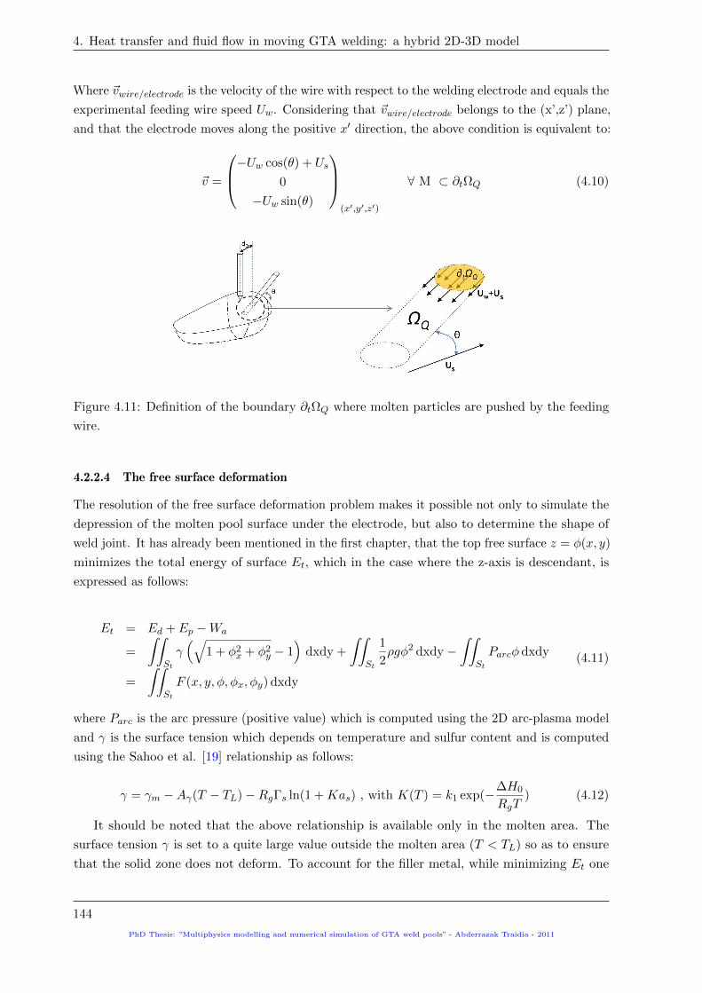
4. Heat transfer and fluid flow in moving GTA welding: a hybrid 2D-3D model
Where ~vwire/electrode is the velocity of the wire with respect to the welding electrode and equals the
experimental feeding wire speed Uw. Considering that ~vwire/electrode belongs to the (x’,z’) plane,
and that the electrode moves along the positive x′ direction, the above condition is equivalent to:
~v =
−Uw cos(θ) + Us
0
−Uw sin(θ)
(x′,y′,z′)
∀ M ⊂ ∂tΩQ (4.10)
Figure 4.11: Definition of the boundary ∂tΩQ where molten particles are pushed by the feeding
wire.
4.2.2.4 The free surface deformation
The resolution of the free surface deformation problem makes it possible not only to simulate the
depression of the molten pool surface under the electrode, but also to determine the shape of
weld joint. It has already been mentioned in the first chapter, that the top free surface z = φ(x, y)
minimizes the total energy of surface Et, which in the case where the z-axis is descendant, is
expressed as follows:
Et = Ed + Ep −Wa
=
∫∫St
γ(√
1 + φ2x + φ2
y − 1)
dxdy +
∫∫St
1
2ρgφ2 dxdy −
∫∫St
Parcφ dxdy
=
∫∫St
F (x, y, φ, φx, φy) dxdy
(4.11)
where Parc is the arc pressure (positive value) which is computed using the 2D arc-plasma model
and γ is the surface tension which depends on temperature and sulfur content and is computed
using the Sahoo et al. [19] relationship as follows:
γ = γm −Aγ(T − TL)−RgΓs ln(1 +Kas) , with K(T ) = k1 exp(−∆H0
RgT) (4.12)
It should be noted that the above relationship is available only in the molten area. The
surface tension γ is set to a quite large value outside the molten area (T < TL) so as to ensure
that the solid zone does not deform. To account for the filler metal, while minimizing Et one
144
PhD Thesis: ”Multiphysics modelling and numerical simulation of GTA weld pools” - Abderrazak Traidia - 2011

4.2. A hybrid 2D-3D modelling
must ensure that the change in the surface shape is linked to the deposited volume ∆Vd using
the following constraint (the first minus sign is due to the orientation of the z-axis):
−∫∫
St
(φ− z0) dxdy =
∫∫St
Gdxdy = ∆Vd (4.13)
where z0 is the z location of the workpiece top surface. Equation 4.13 is equivalent to the
relationship given below which means that the deposited area at the rear of the weld pool is
linked to the rate of metal addition as follows (where rw is the feeding wire radius):
−∫
cross-section(φ− z0) dy =
SwUwUs
=πr2
wUwUs
(4.14)
Finding the solution φ(x, y) that minimizes the total energy Et (equation 4.11) and respects
the constraint expressed in equation 4.13 requires the use of variational calculus. By applying
the Euler-Lagrange criterion, we get:
∂
∂φ(F + λG)− ∂
∂x
[∂
∂φx(F + λG)
]− ∂
∂y
[∂
∂φy(F + λG)
]= 0 (4.15)
After manipulation, we obtain the following partial differential equation1:
− ∂
∂x
γ φx√1 + φ2
x + φ2y
− ∂
∂y
γ φy√1 + φ2
x + φ2y
+ ρgφ = Parc + λ (4.16)
where λ is a Lagrangian multiplier used to satisfy the conservation constraint 4.13.
The resolution of equation 4.16 requires a set of boundary conditions which are given below:
• At the front pool boundary, the surface is undeformed: φ = z0
• At the rear pool boundary, the weld joint is regular:∂φ
∂x= 0
4.2.2.5 Computational domain and boundary conditions
The computational domain used for the 3D weld pool calculations is shown in figure 4.12. It
includes 3 different subdomains; the cylinder ΩQ and two parallelepipeds ΩL and ΩS . The
dimensions of subdomain ΩL are chosen so that it delimits the stationary weld pool. Concerning
the subdomain ΩS , the y′ and z′ dimensions must be respectively the width and height of the
original welded workpiece. However, the x′ dimension can be set to a different value than the
length of the workpiece, since it has been shown in [85] that this dimension does not affect the
computed steady-state solution, but the more the length of ΩS is, the more we get information
about the cooling phase.
1The plus sign in front of λ comes from G = −(φ− z0).
PhD Thesis: ”Multiphysics modelling and numerical simulation of GTA weld pools” - Abderrazak Traidia - 2011
145
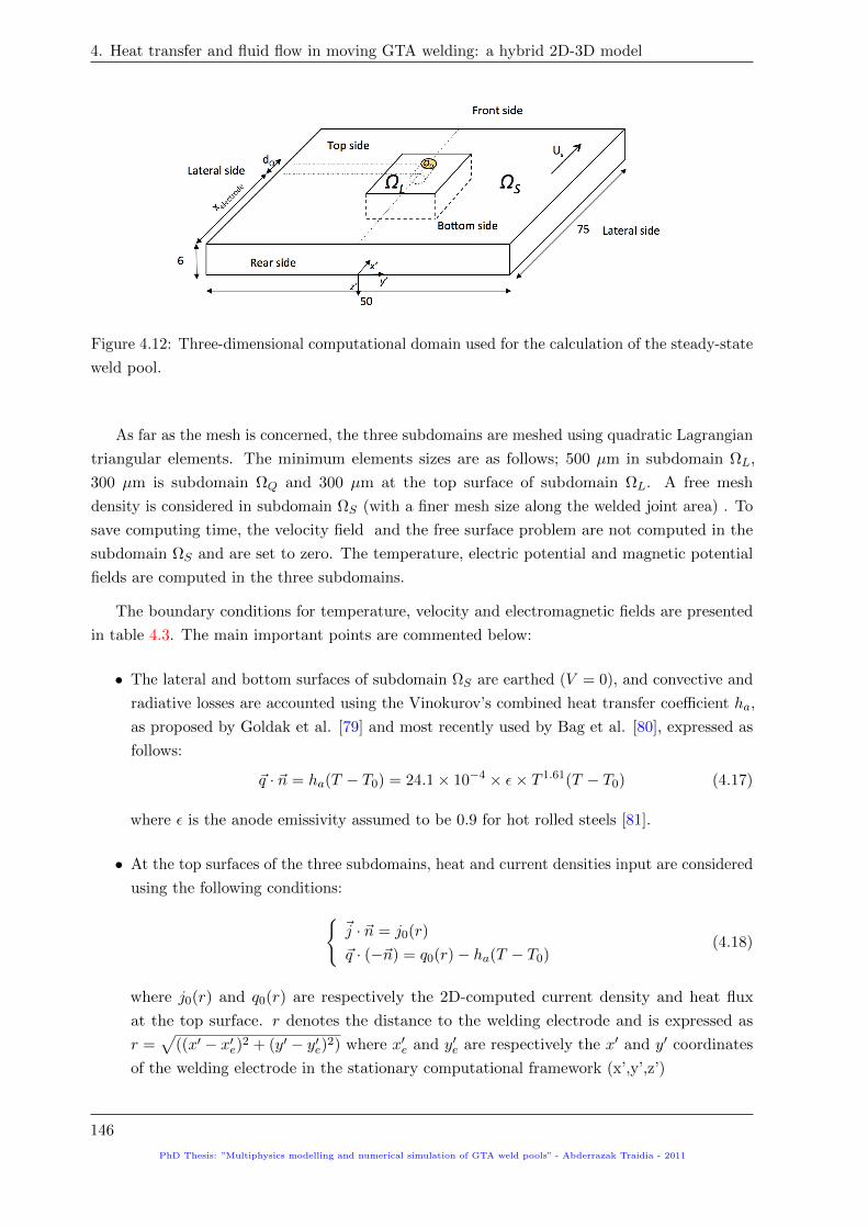
4. Heat transfer and fluid flow in moving GTA welding: a hybrid 2D-3D model
Figure 4.12: Three-dimensional computational domain used for the calculation of the steady-state
weld pool.
As far as the mesh is concerned, the three subdomains are meshed using quadratic Lagrangian
triangular elements. The minimum elements sizes are as follows; 500 µm in subdomain ΩL,
300 µm is subdomain ΩQ and 300 µm at the top surface of subdomain ΩL. A free mesh
density is considered in subdomain ΩS (with a finer mesh size along the welded joint area) . To
save computing time, the velocity field and the free surface problem are not computed in the
subdomain ΩS and are set to zero. The temperature, electric potential and magnetic potential
fields are computed in the three subdomains.
The boundary conditions for temperature, velocity and electromagnetic fields are presented
in table 4.3. The main important points are commented below:
• The lateral and bottom surfaces of subdomain ΩS are earthed (V = 0), and convective and
radiative losses are accounted using the Vinokurov’s combined heat transfer coefficient ha,
as proposed by Goldak et al. [79] and most recently used by Bag et al. [80], expressed as
follows:
~q · ~n = ha(T − T0) = 24.1× 10⁻⁴ × ε× T 1.61(T − T0) (4.17)
where ε is the anode emissivity assumed to be 0.9 for hot rolled steels [81].
• At the top surfaces of the three subdomains, heat and current densities input are considered
using the following conditions:~j · ~n = j0(r)
~q · (−~n) = q0(r)− ha(T − T0)(4.18)
where j0(r) and q0(r) are respectively the 2D-computed current density and heat flux
at the top surface. r denotes the distance to the welding electrode and is expressed as
r =√
((x′ − x′e)2 + (y′ − y′e)2) where x′e and y′e are respectively the x′ and y′ coordinates
of the welding electrode in the stationary computational framework (x’,y’,z’)
146
PhD Thesis: ”Multiphysics modelling and numerical simulation of GTA weld pools” - Abderrazak Traidia - 2011

4.2. A hybrid 2D-3D modelling
• At the top surface of subdomain ΩL (except the top interface ∂tΩQ), the normal velocity
component is set to zero and the Marangoni shear stress is considered as follows: ~v · ~n = 0
µ∇nvs =∂γ
∂T∇sT
(4.19)
• The boundary condition at the top surface of subdomain ΩQ depends on welding conditions;
in the presence of feeding wire (Uw 6= 0) the velocity field is imposed using equation 4.10,
otherwise the Marangoni condition is considered using equation 4.19
• At the front side of ΩS the temperature is set to the ambient temperature T0, and at the
rear side a convective flux boundary condition is considered as follows:
(−k∇T + ρCeqp (T − T0)~Us
)· ~n = 0 (4.20)
T ~v (V, ~A)
Top side of ΩS Eq. 4.18 - Eq. 4.18
Lateral and bottom sides of ΩS Eq. 4.17 - V = 0, ~A× ~n = ~0
Front side of ΩS T = T0 - ~j · ~n = 0, ~A× ~n = ~0
Rear side of ΩS Eq. 4.20 - ~j · ~n = 0, ~A× ~n = ~0
Top side of ΩL Eq. 4.18 Eq. 4.19 Eq. 4.18
Lateral and bottom sides of ΩL - ~v = ~0 -
Front side of ΩL - ~v = ~0 -
Rear side of ΩL - ~v = ~0 -
Top side of ΩQ Eq. 4.18 Eq. 4.10, or Eq. 4.19 Eq. 4.18
Table 4.3: Boundary conditions used for 3D weld pool modelling.
4.2.3 Calculations steps
The flowchart of calculations steps is shown in figure 4.13. The boundary conditions at the top
surface are first computed using the two-dimensional coupled arc/weld-pool model. Then a 3D
calculation of the current density and magnetic field is conducted so as to derive the distribution
of the electromagnetic forces in the 3D domain. Using the previously computed Lorentz forces and
the 2D-computed anodic heat flux, an iterative approach is used to determine the steady-state
temperature and velocity fields, as well as the shape of the weld pool surface. A static ALE
approach is used to ensure a two-way coupling between the thermohydraulic calculations and
the free surface deformation, i.e, the ALE framework is updated at each iteration using the
transformation z′ = φ(x′, y′) at the top surface of the workpiece.
PhD Thesis: ”Multiphysics modelling and numerical simulation of GTA weld pools” - Abderrazak Traidia - 2011
147

4. Heat transfer and fluid flow in moving GTA welding: a hybrid 2D-3D model
Figure 4.13: Flowchart showing the calculations steps.
4.2.4 Materials properties of AISI 316L
The materials properties used for AISI 316L are presented in table 4.4. The evolution with
temperature of density and specific heat of this alloy are shown in figure 4.14. For the thermal
conductivity, we use the same as that used for AISI 304 in the previous chapter shown in figure
3.7.
148
PhD Thesis: ”Multiphysics modelling and numerical simulation of GTA weld pools” - Abderrazak Traidia - 2011

4.2. A hybrid 2D-3D modelling
Symbol Nomenclature Value
Tl Liquidus temperature 1730 K [1]
Ts Solidus temperature 1670 K [1]
Tref Reference temperature 1730 K
ρ0 Reference density 6958 kg m−3
ρLw Wire density at melting temperature 6958 kg m−3
β Thermal expansion coefficient 10−4 K−1 [20]
µ Dynamic viscosity of liquid phase 0.03 kg m−1 s−1 [1]
Lf Latent heat of fusion 2.47 ×10⁵ J Kg−1 [21]
φa Anode work function (without fall voltage) 4.7 V [1]
ε Anode emissivity 0.9 [20]
σ Electrical conductivity 7.7×10⁵ Ω−1 m−1 [1]
as Activity of sulfur 0.003 wt%
∆H0 Standard heat of adsorption -1.88×10⁸ J kmol−1 [12]
Aγ Constant in surface tension gradient 4.3×10⁻⁴ N m−1 K.1 [19]
Rg Gas constant 8314.3 J kmol−1 K−1 [19]
Γs Surface excess at saturation 1.3×10⁻⁸ kmol m−2 [19]
γm Surface tension at pure metal 1.943 N m−1 [19]
k1 Entropy factor 3.18×10⁻³ ([19])
Table 4.4: Material properties used for AISI 316L
Figure 4.14: Evolution with temperature of density (left) and specific heat (right) for AISI 316L
stainless steel.
PhD Thesis: ”Multiphysics modelling and numerical simulation of GTA weld pools” - Abderrazak Traidia - 2011
149

4. Heat transfer and fluid flow in moving GTA welding: a hybrid 2D-3D model
4.3 Numerical Results and discussion
4.3.1 2D-computed boundary conditions
The 2D-computed heat fluxes and current densities at the workpiece surface are shown in figure
4.15. Calculations were done for two levels of welding current (150 A and 200 A) at 2 mm
arc-length. First, we note that the computed solutions have the typical Gaussian distributions
usually used for the approximation of the boundary conditions in GTA and GMA weld pool
models. The heat flux and current densities are higher for the 200 A arc than for the 150 A
arc, due to the higher value of the welding current. Additionally, the area under the heat fluxes
curves, which is representative of the energy transferred to the workpiece, is larger for the higher
arc current. It is about 1070 W for the 150 A arc and 1440 W for the 200 A arc. Considering
that the arc voltage is 10 V, the total energy of the process is 1500 W for the 150 A current and
2000 W for the 200 A current. This means that the process efficiency (defined as the ratio of the
energy transferred to the workpiece to the total process energy) is around 72%, which is in good
agreement with typical values of GTA arcs efficiencies [1].
Figure 4.15: Radial evolution of the computed heat flux and current density at the top surface of
the workpiece for I=150 A and I=200 A, with 2 mm arc-length.
4.3.2 Welding without filler metal
In this section, we simulate numerically the experimentally studied tests 1 and 3. These two
studies were conducted without filler metal (Uw = 0) and respectively with welding currents of
150 A and 200 A. The input operating parameters used in our calculations were previously given
in table 4.1. For the comparison with the experimental results we used a constant value for the
surface tension gradient ∂γ/∂T , since some numerical difficulties were encountered when using a
non-constant value varying with temperature. Indeed, in the case of 200 A welding current with
such a low arc length (2 mm), the mesh size must be refined enough to ensure the convergence of
the fluid flow calculations, which makes the problem beyond the capability of our computers.
However, we will compare the computed steady-state weld pools for the 150 A welding current
(test 1) when using a constant and a temperature-dependent surface tension gradients.
150
PhD Thesis: ”Multiphysics modelling and numerical simulation of GTA weld pools” - Abderrazak Traidia - 2011

4.3. Numerical Results and discussion
4.3.2.1 Steady-state weld pools
Constant surface tension gradient
As the stainless steel workpiece is of low sulfur content (30 ppm), the surface tension gradient is
fixed to the usually used negative value ∂γ/∂T = −1× 10⁻⁴ N m−1 K−1.
Figures 4.16 and 4.17 show the computed steady-state weld pools respectively for test 1 and
test 3. In each figure the top view of temperature and normalized velocity field in the weld pool,
as well as a longitudinal section (1-1) and two cross-sections (2-1) and (2-2) of the weld pool
are shown. The cross-section (2-1) is located at the electrode position, whereas the cross-section
(2-2) is located at the maximum weld pool width.
In both figures, we observe that the fluid flow in the weld pool is outward inducing two loops
that depart from the electrode position where the maximum temperature is located. This is a
direct consequence of the negative value of the surface tension gradient; indeed, the maximum
surface tension occurs at the edges of the weld pool, which forces hot particle to be swept from
the electrode location to the weld pool boundaries, inducing two outward loops. As a consequence
of the molten fluid motion, the temperature field is quite ’spread’ at the top surface (compared
to positive surface tensions flows), with a maximum temperature around 2700 K located under
the welding electrode.
In addition, the front pool boundary is closer to the electrode location than the rear one,
inducing higher thermal gradients at the front of the weld pool (region where (−dT/dx′) > 0).
This is simply the consequence of the welding speed; two consecutive temperature contours
are closer in the region where (−dT/dx′) > 0 (front of the pool) than in the region where
(−dT/dx′) < 0 (rear of the weld pool). Consequently, as seen in the cross-sections (1-1), the rear
outward loop is approximately 3 times larger in size than the front loop.
Concerning the weld pool dimensions, one clearly observes that the molten pool is wider,
longer and deeper for test 3 than for test 1, which is due to the higher value of the welding
current. The maximum weld depth is located near the electrode position, and is about 1.5 mm
for test 1 and 2 mm for test 3. As observed in the cross-sections (2-1), the weld penetration is
relatively increased by the free surface deformation, in particular for test 3 where the high arc
pressure (due to the higher value of the arc current) considerably deforms the top free surface.
The latter observation is in agreement with the conclusions given in the first chapter; i.e., a
two-ways coupling between the free surface deformation and the hydrodynamic calculations is
required when high values of welding currents are considered.
The computed weld shapes for both tests are given in the bottom of figures 4.16 and 4.17.
As observed, due to the low sulfur content of the workpiece ((∂γ/∂T ) < 0), the weld shapes are
wide and shallow, with an average depth-to-width ratio around 22%.
PhD Thesis: ”Multiphysics modelling and numerical simulation of GTA weld pools” - Abderrazak Traidia - 2011
151

4. Heat transfer and fluid flow in moving GTA welding: a hybrid 2D-3D model
z=0 z=0
1 mm
(1-1)
(2-1)
Us
(top view)
z=0
(1-1)
(2-1)(2-2)
z=0
z=0z=0
(2-2)
(weld shape)
w = 6.98 mmL = 7.9 mm
(1-1)
(2-1)(2-2)w
L
Figure 4.16: Steady-state weld pool for test 1 (I=150 A, ∂γ/∂T = −1 × 10⁻⁴ N m−1 K−1).
Temperatures are given in K.
152
PhD Thesis: ”Multiphysics modelling and numerical simulation of GTA weld pools” - Abderrazak Traidia - 2011

4.3. Numerical Results and discussion
z=0 z=0
2 mm
(1-1)
(2-1)
Us
z=0
(1-1)
(2-1)(2-2)
z=0
z=0z=0
(2-2)
(weld shape)
(1-1)
(2-1)(2-2)w
L
(top view)
w = 8.9 mmL = 10.8 mm
Figure 4.17: Steady-state weld pool for test 3 (I=200 A, ∂γ/∂T = −1 × 10⁻⁴ N m−1 K−1).
Temperatures are given in K.
PhD Thesis: ”Multiphysics modelling and numerical simulation of GTA weld pools” - Abderrazak Traidia - 2011
153

4. Heat transfer and fluid flow in moving GTA welding: a hybrid 2D-3D model
Non-constant surface tension gradient
Figure 4.18 shows the computed steady-state weld pool of test 1 (I=150 A) in the case where the
surface tension gradient ∂γ/∂T varies with temperature and sulfur content using the Sahoo et
al. [19] relationship (the values used for this relationship are shown is table 4.4), as well as a
comparison of the longitudinal velocity field at the surface.
First, as concerns the flow directions in the weld pool, a clear difference is observed here
compared to figure 4.16 where a constant surface tension gradient was assumed. Due to the
variation of the surface tension gradient with temperature, and more precisely due to the change
in its sign, four loops coexist simultaneously in the weld pool; two inward loops in the cold region
near the edges of the pool (where ∂γ/∂T > 0) and two outward loops in the hot region near the
electrode (where ∂γ/∂T < 0). Moreover, contrary to stationary GTA weld pools (studied in the
previous chapters), here the inward loops (respectively the outward loops) are not of the same
size. Indeed, as the cooling area of the weld pool (region where (−dT/dx′) < 0) represents the
major part of the molten pool, the two loops occurring in this region are of larger size than the
two loops occurring at the front of the pool.
Analysing the top views of the weld pools shows that the temperature and velocity fields
at the top surface are clearly affected by the varying surface tension gradient. In fact, when
using the Sahoo et al. relationship (with the parameters given in table 4.4) the absolute value
of the surface tension gradient is in the range of 2×10⁻⁴ to 3×10⁻⁴ N m−1 K−1, which means
that the Marangoni shear stress is almost 3 times larger than when using the constant value
∂γ/∂T = −1× 10⁻⁴ N m−1 K−1. This leads to increase the particles velocity at the top surface.
In particular one observes that the maximum velocity for the varying surface tension gradient
pool occurs behind the electrode at the interface where the inward and outward loops join each
other. This is related to the high thermal gradients that occur along this interface inducing
higher level of Marangoni stress. As a consequence, a significant increase in the weld depth
is observed behind the welding electrode, at the interface where the two loops meet. Finally,
another consequence of the varying ∂γ/∂T coefficient is observed on the top view at the rear of
the weld pool, which is closer to a circular shape than to an elliptical one. This modification in
the shape of the molten pool surface is the result of the inward loop occurring at the rear of the
weld pool which tends to move the rear edges toward the welding direction, and then to reduce
the longitudinal length of the molten pool surface.
Comparing the weld shapes given in the bottom of figures 4.16 and 4.18 shows that the
varying ∂γ/∂T coefficient has nearly no effect on the weld width, but slightly increases the weld
pool depth from 1.5 mm to 1.68 mm, which should give a better agreement with the experimental
macrographs.
154
PhD Thesis: ”Multiphysics modelling and numerical simulation of GTA weld pools” - Abderrazak Traidia - 2011

4.3. Numerical Results and discussion
z=0 z=0
1 mm
(1-1)
(2-1)
Us
(top view)
z=0
(1-1)
(2-1)(2-2)
z=0
z=0z=0
(2-2)
(weld shape)
w = 6.93 mmL = 7.4 mm
(1-1)
(2-1)(2-2)w
L
x-component velocity field x-component velocity field4 1 11 10 N.m .K
T
( , )sf T a
T
Figure 4.18: Steady-state weld pool for test 1 with ∂γ/∂T = f(T, as) (top), and comparison of
the computed velocity fields (bottom). Temperatures are given in K and velocities in mm/s.
PhD Thesis: ”Multiphysics modelling and numerical simulation of GTA weld pools” - Abderrazak Traidia - 2011
155

4. Heat transfer and fluid flow in moving GTA welding: a hybrid 2D-3D model
4.3.2.2 Comparison with thermal measurements
Figure 4.19 compares the experimentally measured thermal cycles at the bottom side of the plate
along the fusion line with the numerical predictions for tests 1 and 3. Although we used a 2D
model to get the boundary conditions for the 3D weld pool calculation, the agreement between
the thermal measurements and the computations is satisfying. In particular, one notes that the
maximum temperatures reached are well predicted (about 850 C for test 1 and 1050 C for
test 3). Additionally, the heating rates (slopes of the curves during the heating phase) and the
beginning of the cooling rates (slopes of the curves during the beginning of the cooling phase)
are in good agreement with the experimental measurements.
However, one notes that as far as we leave the welding electrode toward the cooling region of
the weld, a growing discrepancy is observed between the measured temperatures and the numerical
predictions. This means that the numerical model overestimates the cooling rate of the weld.
Besides the errors linked to the numerical side (mesh densities), and to the materials properties
of the stainless steel plates (in particular some different values for the thermal conductivity
are available in the literature), the main sources of explanation could be: the assumption of
axisymmetrical distribution for the heat flux at the workpiece top surface, and the overestimation
of the energy losses at the reverse side of the workpiece. However, a deep analysis of figure 4.19
shows that the discrepancy on the cooling rates appears at least 15 mm behind the welding
electrode, which is approximately 3 times larger than the weld dimensions. This leads to conclude
that the first factor (axisymmetrical heat flux assumption) has certainly no effect on the cooling
rates, since it influences the temperature field just in the region directly close to the weld pool.
The second factor (energy losses) has certainly much more importance on the overestimation of
the cooling rates, it will be discussed later in this chapter.
0
100
200
300
400
500
600
700
800
900
1000
0 20 40 60 80 100
Tem
per
atu
re (
°C)
Axial distance x (mm)
Comparison of thermal cycles on test 1
Temperature distribution at y=0: experiments (TC2)
Temperature distribution at y=0: numerical result
0
200
400
600
800
1000
1200
0 20 40 60 80 100
Tem
per
atu
re (
°C)
Axial distance x (mm)
Comparison of thermal cycles on test 3
Temperature distribution at y=0: experiments (IR)
Temperature distribution at y=0: numerical result
Figure 4.19: Comparison of the measured thermal cycles along the fusion line with the computed
results for test 1 (left) and test 3 (right).
156
PhD Thesis: ”Multiphysics modelling and numerical simulation of GTA weld pools” - Abderrazak Traidia - 2011
4.3. Numerical Results and discussion
4.3.3 Welding with filler metal
In this section, we simulate numerically the experimentally studied test 2 and test 4. These two
studies were conducted in the presence of feeding wire (Uw 6= 0) and respectively with welding
currents of 150 A and 200 A. The input operating parameters used in our calculations were
previously given in table 4.1, and the feeding wire characteristics are the same as those used for
the experimental study (rw = 1 mm, θ = 30 and dQ = 0.5 mm). For the comparison with the
experimental results we set the surface tension gradient to the constant value ∂γ/∂T = −1×10⁻⁴
N m−1 K−1.
4.3.3.1 Steady-state weld pools
Figures 4.20 and 4.21 show the computed steady-state weld pools respectively for test 2 and test
4. First, we note that the fluid flow is still outward, convecting hot particles toward the edges of
the weld pool, which is the result of the negative surface tension gradient. Analysing the top
views of the the weld pool, as well as the sections (1-1) and (2-1) clearly shows that the outward
fluid flow is ’disrupted’ by the presence of the filler metal in the weld pool. Actually, contrary to
tests 1 and 3, where no filler metal was considered, here the outward loops do not join at the
electrode position but are diverted near the region thermally affected by the cold feeding wire.
This is in part the result of the boundary condition imposed at the top surface of the thermally
affected cylinder, and that represents the pushing of the molten pool particles by the feeding
wire during its immersion.
Analysing the different sections of the weld pools and comparing with the results of test 1
and test 3 (welding without filler metal) shows that the introduction of the thermally affected
volume ΩQ produces the expected result. Indeed, the weld pool shape near the region of the
feeding wire immersion is considerably affected by the energy absorption from the filler metal,
and consequently the weld pool depth is significantly decreased in this region. In particular the
decrease in the weld pool depth seems to be less important for the high current case (test 4) than
for the low current one (test 2). To understand this observation, one should compare the rate of
energy losses due to the filler metal Ewire to the total energy transferred to the workpiece. For
the set of operating parameters chosen for the feeding wire, Ewire is found to be around 106 W,
which represents almost 10% of the net welding energy for the 150 A arc current (test 2). As
these 10% losses are located in a quite small area of the weld pool, it locally decreases the weld
pool depth, as observed in figure 4.20.
The decrease in the weld depth seems to be not only the consequence of the energy pumping
from the feeding wire, but is also due to the raise of the top surface at the rear of the weld pool,
which is caused by the metal addition. Actually, as the feeding wire is immersed in the weld pool,
the volume of metal to be heated by the arc plasma becomes more important, and more precisely,
the heat input in the pool region behind the welding electrode occurs at a higher altitude (due
to the formation of the weld joint). This leads to produce less penetrated welds at the rear of
the pool, compared to welds without filler metal.
PhD Thesis: ”Multiphysics modelling and numerical simulation of GTA weld pools” - Abderrazak Traidia - 2011
157

4. Heat transfer and fluid flow in moving GTA welding: a hybrid 2D-3D model
z=0 z=0
1 mm
(1-1)
(2-1)
Us
z=0
(1-1)
z=0
z=0z=0
(2-2)
(weld shape)
z=0
(2-1)(2-2)
(top view)
w = 7.1 mmL = 8.2 mm
(1-1)
(2-1)(2-2)w
L
Figure 4.20: Steady-state weld pool for test 2 (I=150 A, ∂γ/∂T = −1 × 10⁻⁴ N m−1 K−1).
Temperatures are given in K.
158
PhD Thesis: ”Multiphysics modelling and numerical simulation of GTA weld pools” - Abderrazak Traidia - 2011

4.3. Numerical Results and discussion
z=0 z=0
2 mm
(1-1)
(2-1)
Us
z=0
(1-1)
(2-1)(2-2)
z=0
z=0z=0
(2-2)
(weld shape)
z=0
(top view)
w = 9.13 mmL = 10.9 mm
(1-1)
(2-1)(2-2)w
L
Figure 4.21: Steady-state weld pool for test 4 (I=200 A, ∂γ/∂T = −1 × 10⁻⁴ N m−1 K−1).
Temperatures are given in K.
PhD Thesis: ”Multiphysics modelling and numerical simulation of GTA weld pools” - Abderrazak Traidia - 2011
159

4. Heat transfer and fluid flow in moving GTA welding: a hybrid 2D-3D model
Besides the weld depth, the computed results show that the filler metal addition does not really
affect the weld pool width and length. The comparison between test 1 and test 2 (respectively
test 3 and test 4) shows that the molten pool width and length are slightly increased by a
maximum of 0.3 mm. In addition, it should be noted that the weld joint is ’spread’ for test 4,
whilst not for test 3. This is simply because of the weld is wider for the 200 A arc, while the
feeding wire speed is the same than the 150 A arc, which results in a spread weld joint.
4.3.3.2 Comparison with thermal measurements
Figure 4.22 compares the experimentally measured thermal cycles at the bottom side of the plate
along the fusion line with the numerical predictions for tests 2 and 4. Also here, the maximum
reached temperatures, as well as the heating rates are well predicted, however, a discrepancy
on the cooling rates is still observed between the computed results and the experiments; the
numerical model still overestimates the cooling rates at the rear of the weld pool, which is
certainly due to an overestimation of the energy losses at the reverse side of the workpiece.
0
100
200
300
400
500
600
700
800
900
1000
0 20 40 60 80 100
Tem
per
atu
re (
°C)
Axial distance x (mm)
Comparison of thermal cycles on test 2
Temperature distribution at y=0: experiments (TC2)
Temperature distribution at y=0: numerical result
0
200
400
600
800
1000
1200
0 20 40 60 80 100
Tem
per
atu
re (
°C)
Axial distance x (mm)
Comparison of thermal cycles on test 4
Temperature distribution at y=0: experiments (TC2)
Temperature distribution at y=0: numerical result
Figure 4.22: Comparison of the measured thermal cycles along the fusion line with the computed
results for test 2 (left) and test 4 (right).
Figure 4.23 compares the thermal cycles measured at 10 mm from the fusion line (thermocou-
ples TC1 and TC3) with our predicted results. Because of uncertainties related to the locations
of the thermocouples, we also present in figure 4.23 the predicted temperature distributions
along the longitudinal line located at 9 mm from the fusion line. This comparison shows that the
maximum reached values are relatively well predicted, and more particularly when considering
the curves accounting for the uncertainties in the thermocouples locations (y=9 mm). However,
also here the cooling rates are less well predicted than the heating rates. This discrepancy in
the cooling rates which was observed in all the comparisons presented in this chapter has been
attributed to an overestimation of the energy losses at the reverse side of the workpiece. It is
dicussed in the next paragraph.
160
PhD Thesis: ”Multiphysics modelling and numerical simulation of GTA weld pools” - Abderrazak Traidia - 2011

4.3. Numerical Results and discussion
0
100
200
300
400
500
600
0 20 40 60 80 100
Tem
per
atu
re (
°C)
Axial distance x (mm)
Comparison of thermal cycles on test 2
Temperature distribution at y=10 mm: experiments (TC1)
Temperature distribution at y=10 mm: numerical result
Temperature distribution at y=9 mm: numerical result
0
100
200
300
400
500
600
700
800
0 20 40 60 80 100
Tem
per
atu
re (
°C)
Axial distance x (mm)
Comparison of thermal cycles on test 4
Temperature distribution at y=10 mm: experiments (TC1)
Temperature distribution at y=10 mm: numerical result
Temperature distribution at y=9 mm: numerical result
Figure 4.23: Comparison of the measured thermal cycles at 10 mm from the fusion line with the
computed results for test 2 (left) and test 4 (right).
Workpiece emissivity and cooling rate
Heat losses at the reverse side of the workpiece have a direct influence on the temperature field
distribution, and thus on the predicted thermal cycles. In the present work, the heat output at
the reverse side are the sum of the convective and radiative losses and are quantified using the
following relationship:
~q · ~n = ha(T − T0) (4.21)
where ha is called the Vinokurov’s combined heat transfer coefficient, which accounts for both
radiative and convective losses. This combined coefficient depends necessarily on both temperature
and the anode emissivity ε, and is expressed in the literature as follows [79, 80]:
ha = 24.1× 10⁻⁴ × ε× T 1.61 (4.22)
In the above expression, the energy losses are linearly dependent on the value chosen for
the anode emissivity ε. All the results presented before were obtained using ε = 0.9 which is
the value recommended by Touloukian [81] for hot rolled steels. However, the literature review
reveals that this coefficient is not yet fixed, and generally the values used for steels emissivities
vary from 0.4 to 0.9 [85].
Figure 4.24 compares the experimentally measured thermal cycles on test 2 with the numerical
prediction for two values of the workpiece emissivity: ε = 0.4 and ε = 0.9. As expected, it is
found that when using the lower value for the anode emissivity both the maximum reached
temperatures and the cooling rates are better predicted. Indeed, the use of a low value for the
anode emissivity decreases the energy losses, which results in increasing the temperature field at
the reverse side of the workpice and thus the cooling rates. Additionally, as shown in figure 4.25,
where a comparison between the predicted temperature contours for test 2 and the IR measured
PhD Thesis: ”Multiphysics modelling and numerical simulation of GTA weld pools” - Abderrazak Traidia - 2011
161

4. Heat transfer and fluid flow in moving GTA welding: a hybrid 2D-3D model
contours is presented, the agreement is very satisfying, especially when considering the lower
value for the anode emissivity (ε = 0.4).
0
100
200
300
400
500
600
700
800
900
1000
0 20 40 60 80 100
Tem
per
atu
re (
°C)
Axial distance x (mm)
Influence of the workpiece emissivity on the computed results
Temperature distribution at y=0: experiments (TC2)
Numerical prediction: ε=0.9
Numerical prediction: ε=0.4
0
100
200
300
400
500
600
0 20 40 60 80 100
Tem
per
atu
re (
°C)
Axial distance x (mm)
Influence of the workpiece emissivity on the computed results
Temperature distribution at y=10 mm: experiments (TC1)
Numerical prediction: ε=0.9
Numerical prediction: ε=0.4
Figure 4.24: Comparison of the measured thermal with the computed results for test 2, along
the fusion line (left) and 10 mm from the fusion line (right). Influence of the anode emissivity.
550 600 650 700 750 800
10 mmIR measurements
550 600 650 700 750
10 mm Numerical results
550 600 650 700 750 800
10 mmIR measurements
10 mm Numerical results
550 600 650 700 750 800
ε=0.9
ε=0.4
Figure 4.25: Comparison of IR measured temperature contours with the numerical predictions
for the 150 A arc with filler metal (test 2). Influence of the anode emissivity. Temperatures are
given in C.
162
PhD Thesis: ”Multiphysics modelling and numerical simulation of GTA weld pools” - Abderrazak Traidia - 2011

4.4. Conclusion of chapter and limits
4.3.3.3 Comparison with welds macrographs
Figure 4.26 shows a comparison between the numerically predicted weld shapes and the cross-
sections macrographs for the different experimental tests. Globally, the agreement is satisfying,
and more particularly for the 150 A arc current (test 1 and test 2). The welds widths and heights
(w and h) are relatively well predicted, however, some discrepancies are observed on the weld
depths, especially for tests 1 and 3 (welding without filler metal). It should be noted that these
discrepancies can be reduced either by using a surface tension gradient varying with temperature,
or by adjusting another constant value of this coefficient rather than using the classical value
∂γ/∂T = −1× 10⁻⁴ N m−1 K−1.
Figure 4.26: Comparison of the experimental welds macrographs with the numerical predictions
for all the studied tests.
4.4 Conclusion of chapter and limits
In this chapter we have presented an experimental study conducted to investigate the effects
of filler metal addition in a moving GTA weld pool. The experimental results showed that the
feeding wire has nearly no influence on the measured thermal cycles at the reverse side of the
workpiece, whereas it significantly affects the weld shape by decreasing the weld penetration.
This last finding has been attributed to the absorption of energy by the feeding wire from the
hot molten pool.
Using a hybrid 2D-3D approach, a 3D weld pool model was proposed to predict the weld
shape and thermal cycles during moving GTA welding with filler metal. It includes a two-ways
coupling with the free surface deformation and accounts for the filler metal effects on the energy
and momentum balances. The experimental tests have been numerically simulated, and the
computed results show the following findings:
PhD Thesis: ”Multiphysics modelling and numerical simulation of GTA weld pools” - Abderrazak Traidia - 2011
163

4. Heat transfer and fluid flow in moving GTA welding: a hybrid 2D-3D model
• The use of a negative constant surface tension gradient results in two outward loops in
the weld pool convecting hot particles toward the edges of the weld. The loop occurring
behind the weld electrode is nearly 3 times larger in-size than that occurring at the front
pool region, which is the direct consequence of the temperature contours that become more
spaced at the rear of the weld pool due to the moving electrode.
• The use of a temperature-dependent surface tension gradient induces four loops in the weld
pool corresponding to the regions where this coefficient is either positive or negative. The
two loops occurring behind the welding electrode are of larger size, and join each other
near the rear edge of the pool which leads to increase the weld depth in this region.
• In the presence of filler metal, the numerical results show that the weld depth is locally
decreased in the region thermally affected by the feeding wire, especially for the low current
weld (I=150 A) where the energy absorbed by the wire is almost 10% of the total energy
transferred to the workpiece.
• Despite the use of a two-dimensional model for the determination of the boundary conditions
at the workpiece surface, the weld shapes, maximum reached temperatures and thermal
cycles are relatively well predicted. However, the numerical results overestimate the cooling
rates at the rear of the welding electrode, which has been numerically found to be linked to
the value chosen for the anode emissivity.
Besides the 2D computation of the boundary conditions at the workpiece surface, the main
improvement that should be considered in the near future is to include the feeding wire in the
computational domain and to deal with the whole problem in a unified formalism. This would
overcome the assumption of an arbitrary volume ΩQ thermally affected by the feeding wire in
the weld pool.
164
PhD Thesis: ”Multiphysics modelling and numerical simulation of GTA weld pools” - Abderrazak Traidia - 2011

Chapter 5
Application to horizontal GTA welding
This chapter gives an experimental and numerical analysis of the
weld pool behaviour and the resulted weld shape during
horizontal-position GTAW. After validating the numerical results
for bead-on-plate cases, the numerical model is used to simulate
Narrow-Gap Horizontal-position GTAW. The asymmetries in the
lateral penetrations are identified both, experimentally and
numerically. An extension to dissimilar sulfur content welds is
presented.
Contents
5.1 Experimental study . . . . . . . . . . . . . . . . . . . . . . . . . . . . . . . . . . . 167
5.1.1 Experimental set-up . . . . . . . . . . . . . . . . . . . . . . . . . . . . . . . 167
5.1.2 Results and discussion . . . . . . . . . . . . . . . . . . . . . . . . . . . . . . 168
5.2 Numerical simulation . . . . . . . . . . . . . . . . . . . . . . . . . . . . . . . . . . . 170
5.2.1 Accounting for the gravity effects . . . . . . . . . . . . . . . . . . . . . . . . 170
5.2.2 Geometry and boundary conditions . . . . . . . . . . . . . . . . . . . . . . . 172
5.2.3 Numerical results . . . . . . . . . . . . . . . . . . . . . . . . . . . . . . . . . 173
5.2.4 Comparison with experiments . . . . . . . . . . . . . . . . . . . . . . . . . . 177
5.3 Application to NGH-GTAW . . . . . . . . . . . . . . . . . . . . . . . . . . . . . . . 179
5.3.1 Computational domain and boundary conditions . . . . . . . . . . . . . . . 179
5.3.2 Numerical results . . . . . . . . . . . . . . . . . . . . . . . . . . . . . . . . . 181
PhD Thesis: ”Multiphysics modelling and numerical simulation of GTA weld pools” - Abderrazak Traidia - 2011
165

5.3.3 Extension to dissimilar sulfur contents welds . . . . . . . . . . . . . . . . . 183
5.4 Conclusion . . . . . . . . . . . . . . . . . . . . . . . . . . . . . . . . . . . . . . . . 187
166
PhD Thesis: ”Multiphysics modelling and numerical simulation of GTA weld pools” - Abderrazak Traidia - 2011

5.1. Experimental study
5.1 Experimental study
In this section, we present the results of an experimental investigation conducted during horizontal-
position GTA welding (hereafter called horizontal welding) of stainless steel plates. Three main
objectives are targeted by this study:
• Analysing the effects of the welding position on the thermal field distribution at the reverse
side of the workpiece.
• Identifying a possible asymmetry in the weld shapes, as well as the direction in which it
occurs.
• Improving the previously developed hybrid 2D-3D model to account for the asymmetric
effects of gravity during horizontal welding . The numerical predictions will be compared
with the experimental results for validation.
5.1.1 Experimental set-up
As shown in figure 5.1, we used the same experimental set-up as the previous chapter, except for
the welding position that was changed to a horizontal one.
Weld joint
IR camera
Computer
Weldingtorch g
Figure 5.1: Experimental set-up used for the study of horizontal GTAW with filler metal.
As concerns the welding parameters, we realised two bead-on-plate welds with two different
welding currents. For each weld we considered the welding parameters used in the previous
chapter for tests 2 and 4. Table 5.1 summarizes these parameters, as well as the designation of
each test. The feeding wire and workpiece characteristics (material and dimensions) are the same
as the previous chapter.
PhD Thesis: ”Multiphysics modelling and numerical simulation of GTA weld pools” - Abderrazak Traidia - 2011
167
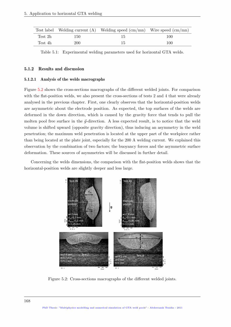
5. Application to horizontal GTA welding
Test label Welding current (A) Welding speed (cm/mn) Wire speed (cm/mn)
Test 2h 150 15 100
Test 4h 200 15 100
Table 5.1: Experimental welding parameters used for horizontal GTA welds.
5.1.2 Results and discussion
5.1.2.1 Analysis of the welds macrographs
Figure 5.2 shows the cross-sections macrographs of the different welded joints. For comparison
with the flat-position welds, we also present the cross-sections of tests 2 and 4 that were already
analysed in the previous chapter. First, one clearly observes that the horizontal-position welds
are asymmetric about the electrode position. As expected, the top surfaces of the welds are
deformed in the down direction, which is caused by the gravity force that tends to pull the
molten pool free surface in the ~g-direction. A less expected result, is to notice that the weld
volume is shifted upward (opposite gravity direction), thus inducing an asymmetry in the weld
penetration; the maximum weld penetration is located at the upper part of the workpiece rather
than being located at the plate joint, especially for the 200 A welding current. We explained this
observation by the combination of two factors; the buoyancy forces and the asymmetric surface
deformation. These sources of asymmetries will be discussed in further detail.
Concerning the welds dimensions, the comparison with the flat-position welds shows that the
horizontal-position welds are slightly deeper and less large.
2mm
2
m
m
10 : 1
w=7.4 mmd=0.7 mmh=1.1 mm
Test 2
2mm
2
m
m
10 : 1
h
d
w
w=9.1 mmd=2 mmh=1 mm
Test 4
2m
m
2mm
10
: 1
2m
m
2mm
10
: 1 Test 4hTest 2h
g
Electrode position
Electrode position
dup
ddown
w=7 mmdup=1.7 mmddown=1.5 mmh=1.25 mm
w=7.9 mmdup=2.1 mmddown=1.45 mmh=1.1 mm
Figure 5.2: Cross-sections macrographs of the different welded joints.
168
PhD Thesis: ”Multiphysics modelling and numerical simulation of GTA weld pools” - Abderrazak Traidia - 2011

5.1. Experimental study
5.1.2.2 Thermal effects of gravity
The influence of horizontal welding position on the temperature measurements at the reverse
side of the workpiece are presented in figure 5.3, in which we compare the temperature contours
for tests 2 and 2h (I=150 A). First, one notes that although the weld shape was found to be
asymmetric for test 2h, the temperature field at the reverse side remains symmetrical about
the fusion line. This means that the different factors that cause the weld asymmetry have an
influence on the temperature field just in a small area around the weld pool, as far as we leave
this region, the temperature field becomes symmetrical.
Comparing the two cases shows that the maximum temperatures reached are nearly the
same, and are around 800C for both cases. However, one notices that the temperature contours
are more spaced in the longitudinal direction for the flat-position weld than for the horizontal-
position one, which suggests saying that less energy is transferred towards the bottom side during
horizontal GTAW. This has also been observed for the 200 A arc when comparing test 4 with
test 4h. However, it should be noted that the latter result is to be considered with cautiousness,
since to avoid the dispersions linked to the experimental side, the tests should have been done
several times to validate this observation.
550 °C
650 °C
750 °C
800 °C
10 mm Position of the welding electrode
Test 2 (flat GTAW)
Test 2h (horizontal GTAW)
Figure 5.3: Influence of welding position on the temperature field at the reverse side of the
workpice.
PhD Thesis: ”Multiphysics modelling and numerical simulation of GTA weld pools” - Abderrazak Traidia - 2011
169

5. Application to horizontal GTA welding
5.2 Numerical simulation
In this section we intend to use the hybrid 2D-3D model presented in the previous chapter, to
simulate numerically the experimental tests 2h and 4h. We aim to identify the asymmetries
observed in the cross-sections of the welds, and to emphasize the role of buoyancy forces and the
free surface deformation on the resulting weld shapes.
5.2.1 Accounting for the gravity effects
The mathematical model to be used in this study has already been presented in the previous
chapter, here, we only have to modify the equations affected by the asymmetric effects of the
gravity force, i.e, the conservation of momentum and the free surface deformation.
5.2.1.1 Influence of welding position on the momentum balance
The equation of momentum conservation given in the previous chapter is reminded below:
ρ(~v − ~Us
)· ∇~v = −∇p+∇ ·
[µ(∇~v +t ∇~v)
]+~j × ~B + ρ0 (1− β(T − Tref ))~g (5.1)
As the above equation is given in its vectorial formalism, the influence of changing the welding
position is automatically included in the definition of vector ~g. Indeed, as shown in figure 5.4, to
simulate horizontal-position welding one only needs to change the direction of ~g from ~z′ to ~y′.
This is very simple since the computational domain and the boundary conditions remain the
same as for flat-position simulations.
In this study we only focus on the simulation of horizontal GTAW, however, it should be
mentioned that the above approach can be applied to any other welding position by parametrizing
the gravity vector ~g with two independent angles α1 and α2.
Figure 5.4: Three-dimensional computational domain used for the study of horizontal GTAW.
5.2.1.2 Influence of welding position on the free surface shape
As concerns the free surface shape, the model proposed in the previous chapter can no longer be
used, since the gravitational potential energy Ep should be expressed differently when changing
170
PhD Thesis: ”Multiphysics modelling and numerical simulation of GTA weld pools” - Abderrazak Traidia - 2011

5.2. Numerical simulation
the welding position. Figure 5.5 shows the studied configuration in the case of horizontal-position
welding. To be coherent with the studies available in the literature, it is worth noting that the
free surface model is here given for a z-axis directed downward (toward the reverse side of the
workpiece).
z
y
gravity
z=φ(x,y)
OSL
Figure 5.5: Schematic representation of the free surface shape in horizontal GTAW.
At the equilibrium, the free surface shape z = φ(x, y) minimizes the total potential energy
of free surface Et (which is the sum of the surface deformation energy Ed, the gravitational
potential energy Ep and the arc pressure energy Ea). The expressions of the surface deformation
and arc pressure energies are not dependent on the welding position and are still given as follows:
Ed + Ea = Ed −Wa =
∫∫St
γ(√
1 + φ2x + φ2
y − 1)
dxdy −∫∫
St
Parcφ dxdy (5.2)
where Parc is the arc pressure (positive value) computed using the two-dimensional arc plasma
model.
As concerns the gravitational potential energy Ep of the volume V located under the free
surface, it is computed as follows:
Ep = −∫∫∫
Vρ~g · ~OM dV
= −∫∫∫
Vρ(g~y) · (x~x+ y~y + z~z) dV
= −∫∫∫
Vρgy dV
= −∫∫
St
[∫ 0
φ(x,y)ρgy dz
]dxdy
=
∫∫St
ρgyφdxdy
(5.3)
PhD Thesis: ”Multiphysics modelling and numerical simulation of GTA weld pools” - Abderrazak Traidia - 2011
171

5. Application to horizontal GTA welding
Then, the total energy of surface Et is expressed as following:
Et = Ed + Ep −Wa
=
∫∫St
γ(√
1 + φ2x + φ2
y − 1)
dxdy +
∫∫St
ρgyφdxdy −∫∫
St
Parcφ dxdy
=
∫∫St
F (x, y, φ, φx, φy) dxdy
(5.4)
As discussed in the previous chapter, accounting for the filler metal leads to verify the
following additional constraint (the first minus sign is due to the orientation of the z-axis):
−∫∫
St
(φ− z0) dxdy =
∫∫St
Gdxdy = ∆Vd (5.5)
By applying the Euler-Lagrange criterion, we get:
∂
∂φ(F + λG)− ∂
∂x
[∂
∂φx(F + λG)
]− ∂
∂y
[∂
∂φy(F + λG)
]= 0 (5.6)
After manipulation, we obtain the following partial differential equation that governs the free
surface shape in horizontal-position welding:
− ∂
∂x
γ φx√1 + φ2
x + φ2y
− ∂
∂y
γ φy√1 + φ2
x + φ2y
+ ρgy = Parc + λ (5.7)
The above equation can be written in the following classical form:
−∇ · (c∇u) + au = f (5.8)
where u is the unknown variable (here, u = φ), c, a and f are identified from equation 5.7:
c =γ√
1 + φ2x + φ2
y
a = 0
f = Parc − ρgy + λ
(5.9)
It is worth mentioning that the previous described calculations can be done for any other
welding position; one only needs to parametrise the position of ~g by two angles α1 and α2 in
equation 5.3, and then to derive the corresponding PDE using the Euler-Lagrangian criterion.
More details about this generalisation of the model can be found in the appendix C.
5.2.2 Geometry and boundary conditions
The computational domain and boundary conditions used in this study are the same as the
previous chapter. The anode emissivity is set to ε = 0.4, since it has been shown in the previous
chapter that this value gives a good agreement when comparing the numerical predictions with
the measured thermal cycles at the reverse side of the workpiece.
172
PhD Thesis: ”Multiphysics modelling and numerical simulation of GTA weld pools” - Abderrazak Traidia - 2011

5.2. Numerical simulation
5.2.3 Numerical results
5.2.3.1 Analysis of the steady-state weld pools
Figures 5.6 and 5.7 show the computed steady-state weld pools respectively for test 2h and test
4h. In each figure it is represented the top view of the temperature and normalized velocity
fields in the weld pool, as well as a longitudinal section (1-1) and two cross-sections (2-1) and
(2-2) located respectively at the electrode position and at the maximum weld pool width. The
direction of gravity in each figure is represented by ~g.
First of all, it is remarkable to note that the cross-sections of the weld pool are clearly
asymmetric about the electrode position. Analysing the different cross-sections as well as the
computed weld shapes shows that the numerical results give the same conclusions as shown
experimentally concerning the weld macrographs; i.e., the weld surface is deformed towards the
gravity direction, while the weld pool is more penetrated in the upper part of the weld. Indeed,
these two phenomena are closely linked; as the gravity force pulls the free surface downward,
more liquid metal is shifted towards the gravity direction, which causes the swelling of the weld
in this region. As a consequence, the heat input in the upper part of the weld pool occurs at
lower altitude than in the bottom part, which increases the weld penetration in the upper part
and induces the observed asymmetry in the weld shape.
Additionally, the asymmetry of the weld shape seems to be much more pronounced for test 4h
than for test 2h. To understand this fact, one should remember that the arc pressure is greater
for the 200 A arc, which means that the upper part of the weld pool is much more deformed
than for the 150 A arc (as observed in the cross-sections 2-2). This leads to a significant increase
in the weld depth on the upper part, which enhances the asymmetry of the weld.
However, the asymmetry in the weld depth is not only the consequence of the free surface
being deformed downward, but is also due to the fluid flow directions. Indeed, an in-depth analysis
of the fluid flow in the cross-sections (2-2) shows that molten metal is more directed towards
the opposite gravity direction, especially near the top free surface. This is the consequence of
the buoyancy force that tends to convect hot fluid towards the opposite gravity direction. As
the magnitude of the buoyancy force is proportional to the temperature difference (T − Tref ), it
is more important near the top surface, which explains the observed results. This argument is
confirmed in figure 5.8, where the maximum values of the different components of the velocity
field are shifted upward. A more detailed analysis of the buoyancy-induced flow is presented in
the next section.
Concerning the weld pool dimensions, the comparison with the flat-position simulations shows
a slight increase by a maximum of 0.3 mm for horizontal welds.
PhD Thesis: ”Multiphysics modelling and numerical simulation of GTA weld pools” - Abderrazak Traidia - 2011
173

5. Application to horizontal GTA welding
1 mm
(1-1)
(2-1)
Us
z=0
(1-1)
(2-1)(2-2)
z=0
z=0
(weld shape)
w = 7.08 mmL = 8.2 mm
(1-1)
(2-1)(2-2)w
L
g
(2-2)
g
(Top view)
Figure 5.6: Steady-state weld pool for test 2h (I=150 A, ∂γ/∂T = −1 × 10⁻⁴ N m−1 K−1).
Temperatures are given in K.
174
PhD Thesis: ”Multiphysics modelling and numerical simulation of GTA weld pools” - Abderrazak Traidia - 2011

5.2. Numerical simulation
(1-1) Us
(top view)
z=0
(1-1)
(2-1)(2-2)
z=0
(2-2) (weld shape)
w = 9.04 mmL = 11.2 mm
(1-1)
(2-1)(2-2)w
L
g
z=0 z=02 mm
(2-1)
g
Figure 5.7: Steady-state weld pool for test 4h (I=200 A, ∂γ/∂T = −1 × 10⁻⁴ N m−1 K−1).
Temperatures are given in K.
PhD Thesis: ”Multiphysics modelling and numerical simulation of GTA weld pools” - Abderrazak Traidia - 2011
175

5. Application to horizontal GTA welding
x-component velocity field y-component velocity field Norm velocity field
g g g
Figure 5.8: Computed velocity field at the top surface of the weld pool for test 2h (velocity values
are given in mm/s).
5.2.3.2 The buoyancy-induced flows
Previously, we suspected the buoyancy effect to be in part responsible for the asymmetries
observed in horizontal GTA welds, with the argument that it creates upward flows. To emphasize
this fact, this section is devoted to the analysis of the fluid flow directions and the resultant weld
shapes induced by only the buoyancy force in the weld pool.
Figure 5.9 shows the computed steady-state weld pools in the virtual case where only
the buoyancy force is governing the fluid flow in the weld pool (no Marangoni stress and no
electromagnetic forces). For comparison, we did two numerical simulations with flat and horizontal
welding positions. The welding current is fixed at 150 A for both studies.
As expected for the flat-position weld pool, the liquid metal is pushed upward along the weld
pool axis then hot fluid is convected outward to the pool boundary. This is the consequence
of the metal density that decreases with increasing temperature, which causes warmer metal
located at the weld pool center to rise and cooler fluid located at the pool boundary to sink.
This creates two outward loops that join each other along the gravity direction (which is in
this case the weld pool axis). Due to this symmetrical fluid flow, the surface temperature, as
well as the final weld shape are perfectly symmetrical about the fusion line. In this regard, it
should be mentioned that the maximum reached temperature is around 3300 K for both studies
and then is approximately 700 K higher than for the complete simulations (accounting for the
Marangoni and electromagnetic effects), which is due to the low values of velocity field induced
when accounting only for the buoyancy force.
As concerns the horizontal GTA weld pool, the fluid flow is completely different from the
previously described flow. The physical phenomenon behind is still the same; i.e., the warm liquid
at the weld pool center is lighter and then rises along the gravity axis, whereas the cool liquid
at the pool boundary is heavier and sinks. However, as the gravity axis is here different from
the electrode axis, the two induced loops join each other, thus creating a single upward loop at
the middle cross-section. As a consequence, the temperature field in the weld pool is completely
176
PhD Thesis: ”Multiphysics modelling and numerical simulation of GTA weld pools” - Abderrazak Traidia - 2011

5.2. Numerical simulation
asymmetric about the fusion line, in particular one notices that the maximum pool temperature
location shifts towards the opposite gravity direction. The main impact of the buoyancy-induced
flow in horizontal GTAW is observed on the resultant weld shape; the maximum weld penetration,
as well as about two-thirds of the molten zone are located in the upper part of the workpiece.
This results confirms the conclusion given in the first chapter about the role of buoyancy force in
the weld asymmetries in Narrow-Gap Horizontal-position GTAW (NGH-GTAW).
g
Electrode position
Horizontal position
1 mm
Flat position
(Top view)
(cross-section at maximum weld depth)
(weld shape)
Electrode position
g
g
g
gg
Figure 5.9: Influence of the welding position on the buoyancy-induced flow for I=150 A. Temper-
atures are given in K.
5.2.4 Comparison with experiments
5.2.4.1 Thermal measurements
The computed temperature contours at the bottom workpiece surface for test 2h are compared
with the IR measurements in figure 5.10. The maximum reached values as well as the widths of
the temperature contours are relatively well predicted. Here, it is also found that the lengths
of the temperature contours are consistent with the experimental measurements, which means
that the cooling rates are well predicted. This is the consequence of the low value used for the
workpiece emissivity ε = 0.4.
PhD Thesis: ”Multiphysics modelling and numerical simulation of GTA weld pools” - Abderrazak Traidia - 2011
177

5. Application to horizontal GTA welding
550 600 650 700 750 800
10 mm 10 mm Numerical resultsIR measurements
550 600 650 700 750 800
ε=0.4
Figure 5.10: Comparison of IR-measured temperature contours with experimental predictions for
test 2h. Temperatures are given in C.
5.2.4.2 Welds macrographs
Figure 5.11: Comparison of the experimental welds macrographs with the numerical predictions
for tests 2h and 4h.
Figure 5.11 compares the numerically predicted weld shapes with the cross-sections macrographs
for tests 2h and 4h. Globally, the agreement is satisfying, and more particularly for the welds
widths and heights (w and h). However, some discrepancies are observed on the weld depths,
especially for the 150 A arc. This can be attributed to different factors; first, as the top free surface
178
PhD Thesis: ”Multiphysics modelling and numerical simulation of GTA weld pools” - Abderrazak Traidia - 2011

5.3. Application to NGH-GTAW
is deformed downward, the heat flux at the workpiece surface can differ from that computed by
the two-dimensional model, since the latter does not account for the free surface deformation. In
addition, the complex phenomena that occur during the immersion of the feeding wire in the
weld pool, such as the appearing of new vortices and the mixing of cold feeding wire with hot
molten pool are not modelled, which could certainly have major influence on the resultant weld
shape.
5.3 Application to NGH-GTAW
In the first chapter, we used a two-dimensional weld pool model to analyse a virtual welding
operation ’representative’ of NGH-GTAW, and found that the buoyancy force is in part responsible
for the weld defects observed experimentally. However, as real NGH-GTAW situations need
a three-dimensional weld pool model to be studied, the 2D-computed results needed further
confirmation.
In the previous sections we showed that the combination of buoyancy forces and asymmetric
surface deformation are responsible of the weld asymmetries for bead-on-plate welds. This
suggests saying that the same phenomena should occur when the workpiece geometry is different.
To confirm the results of the first chapter, we intend here to use the three-dimensional model
developed in this chapter to compute the weld shape in NGH-GTAW.
5.3.1 Computational domain and boundary conditions
To simplify the problem and to easy the convergence, we do not account in this study for the
energy losses due to the filler metal addition, since the main goal here is to investigate a possible
weld asymmetry due to the horizontal welding position. As a consequence, the computational
domain used in this study, shown in figure 5.12, does not include the thermally-affected volume
ΩQ. Additionally, one notes that we used an angled-chamfer (which differs slightly from a
real narrow gap), since to compute the free surface deformation using the energy minimization
approach, one needs to get a bijection between the chamfer surface ∂cΩS and the x-y plane.
The boundary conditions imposed at the front, rear, lateral and bottom sides are the same as
the previous chapter and were given in table 4.3. As concerns the top surface, convection and
radiation losses are taken into account using the Vinokurov’s combined heat transfer coefficient.
Heat and current inputs are considered at the chamfer boundary.
On the groove boundary ∂gΩ, the normal velocity is zero and the Marangoni shear stress
is taken into account. Contrary to bead-on-plate welds, here the two-dimensional arc plasma
model can no longer be used to compute the boundary conditions j0(x, y, z) and q0(x, y, z) on
the groove boundary. Indeed, as the curvature of this surface is important, one needs a true
three-dimensional arc plasma model to determine with accuracy the arc attachment as well as the
energy transferred to the workpiece. In this study we propose the following analytical expressions
PhD Thesis: ”Multiphysics modelling and numerical simulation of GTA weld pools” - Abderrazak Traidia - 2011
179

5. Application to horizontal GTA welding
for the heat flux and current density:
~q · (−~n) =dUIη
πa20
exp
(−dr
2
a20
)exp
(−d(z − ze)2
2b20
)− ha(T − T0)
~j · ~n =dI
πa20
exp
(−dr
2
a20
)exp
(−d(z − ze)2
2b20
) (5.10)
where d is the distribution factor, U is the welding voltage, I is the welding current, η is the process
efficiency, r =√
[(x− xe)2 + (y − ye)2] is the radial distance from an arbitrary point M(x, y, z)
to the electrode location E(xe, ye, ze) and a0, b0, xe, ye and ze are geometrical parameters as
specified in figure 5.12.
The analytical expressions proposed in Eq. 5.10 are quite similar to the analytical Gaussian
distributions usually used in the literature for welding on plates, except that we added a new
term that decreases exponentially with z, and represents the heating of the lateral sides of the
chamfer. Additionally, the analytical expressions proposed here are conservative, i.e;∫∂cΩS
[~q · (−~n) + ha(T − T0)] dS ' UIη∫∂cΩS
~j · ~ndS ' I(5.11)
Concerning the free surface deformation, the model previously proposed for bead-on-plate
welds is still valid and can be used for any workpiece geometry (plates, narrow-gap, fillet, etc.).
Also the associated boundary conditions remain the same as for plates, with a particular attention
that for complex geometries, the top surface location z0 (parameter appearing in the expression
of the volume-conservation boundary conditions) is not constant but depends on coordinates
(x,y), as shown in figure 5.13.
!g"
50
35
12
E(xe , ye , ze )
zo(x, y)
xy
z Gravity 2a0
2b0 Us
Figure 5.12: Three-dimensional computational domain used to calculate the steady state weld
pool. Dimensions are in (mm).
180
PhD Thesis: ”Multiphysics modelling and numerical simulation of GTA weld pools” - Abderrazak Traidia - 2011

5.3. Application to NGH-GTAW
!g" zo(x, y)
Gravity
A B
C D
y
x
Figure 5.13: Two dimensional computational domain (yellow) used to compute the free surface
shape. Dimensions are in (mm).
5.3.2 Numerical results
The operating parameters used for the simulations are given in table 5.2 below:
Symbol Nomenclature Value
I welding current 200 A - 250 A
U welding voltage 10 V
η process efficiency 0.72
d distribution parameter 3
a0 half-opening of the chamfer 5 mm
b0 half-height of the chamfer 3 mm
xe x-coordinate of the welding electrode 17.5 mm
ye y-coordinate of the welding electrode 25 mm
ze z-coordinate of the welding electrode 6 mm
Us welding speed 10 cm/min
Uw feeding wire speed 70 cm/min - 100 cm/min
rw Wire radius 0.5 mm
∂γ/∂T surface tension gradient -1×10⁻⁴ N m−1 K−1
Table 5.2: Operating parameters used for the simulation of NGH-GTAW.
Figure 5.14 shows the weld shapes computed for three sets of operating parameters, as well
as an experimental weld macrograph 1 for a qualitative comparison. As expected, the different
1This weld macrograph corresponds to pulsed current NGH-GTAW, and was kindly provided by the technical
center AREVA NP.
PhD Thesis: ”Multiphysics modelling and numerical simulation of GTA weld pools” - Abderrazak Traidia - 2011
181

5. Application to horizontal GTA welding
bead shapes are asymmetric about the groove centreline, with larger penetration in the upper
sidewall. Indeed, due to the action of gravity on the pool free surface, the solidified weld surface
is sagged towards the bottom pipe, which leads to more metal in this region of the weld. As a
consequence, the heat input in the upper part of the weld pool occurs close to the initial chamfer
(black dashed line). This factor combined to the upward buoyancy-induced flows (discussed in
the previous section) tend to increase the upper sidewall penetration.
Comparing the two first simulations shows that the increase in the feeding wire speed increases
the weld volume and slightly decreases the lateral penetrations on both parts of the chamfer.
Additionally, the comparison of the two last simulations shows that an increase in the welding
current by 25% increases considerably both the weld volume and the lateral penetrations. Indeed,
for the 200 A welding current, the ratio of the maximum upper penetration to the bottom one
is around 1.5 while it increases to 2 for the 250 A arc. This result is induced by two factors;
first, enhancing the welding current leads to melt more metal especially on the lateral sides of
the chamfer, and therefore more metal is sagged towards the bottom part of the weld, thereby
facilitating the melting in the upper part. Furthermore, as the buoyancy force is proportional to
the temperature difference (T −Tref ), the increase in the welding current amplifies the magnitude
of the upward buoyancy-induced flow which increases the weld penetration in the upper part.
This result is quite important, since it suggests that during NGH-GTAW with pulsed current
mode (which is the case in industrial applications), the weld asymmetry occurs mainly during
the peak pulse duration, since the welding current is increased.
The comparison between the 250 A welding current simulation and the experimental macro-
graph shows qualitatively a good agreement; the lateral penetration is larger in the upper sidewall
and the weld surface is sagged downward. In addition, one notes that the wetting angle in the
upper part is larger than that in the bottom one (both experimentally and numerically), which
is the consequence of the free surface being sagged downward. Also, it is worth mentioning that
our numerical simulation corresponds to the first pass of welding, which means that the initial
chamfer geometry is considred to be perfectly symmetrical about the centreline (contrary to the
following passes). Consequently, the weld shapes calculated for the following passes would be
much more asymmetric than that computed for the first pass, since the initial geometry of the
chamfer would be asymmetric and more metal has to be melted in the bottom part of chamfer.
182
PhD Thesis: ”Multiphysics modelling and numerical simulation of GTA weld pools” - Abderrazak Traidia - 2011

5.3. Application to NGH-GTAW
I=200 A Uw=70 cm/mn I=200 A Uw=100 cm/mn I=250 A Uw=100 cm/mn
0.9
0.63
0.82
0.56
1.4
0.76
2 mmg
Chamfer
Figure 5.14: Computed weld shapes for the different studied cases of NGH-GTAW (top), and
qualitative comparison with a narrow-gap weld macrograph (bottom).
5.3.3 Extension to dissimilar sulfur contents welds
We previously showed that the issue of asymmetric welds in NGH-GTAW is due to the combination
of the upward buoyancy-induced flow, and the sagging of the weld top surface. To deal with this
issue, it is easier to act on the fluid flow directions than on the free surface deformation, since the
latter is mainly governed by the gravity force that pulls the surface towards the gravity direction.
Actually, one can imagine to balance the upward buoyancy flow, either by modifying the
heating conditions (for example by inclining the welding electrode towards the bottom pipe, or
by using new techniques such as rotating/swing arc systems [86, 87]), or by creating an external
PhD Thesis: ”Multiphysics modelling and numerical simulation of GTA weld pools” - Abderrazak Traidia - 2011
183

5. Application to horizontal GTA welding
effect (for example using an electromagnetic force) that tends to shift the weld pool downward.
To achieve this, we were inspired by the recent work of Mishra et al. [8] in which they studied
GTAW of stainless steel plates with dissimilar sulfur concentrations and flat welding position.
Their investigation mainly showed the following conclusions:
• The weld bead is shifted towards the lower sulfur content plate with less melting on the
high sulfur side, often resulting in a weld with a missed joint (see figure 5.15 left).
• The point of maximum penetration is also shifted towards the plate containing lower sulfur.
• Videos taken during the experiments showed an asymmetry of the arc for dissimilar sulfur
welds, with flaring out of the arc towards the low sulfur plate just above the workpiece
surface (see figure 5.15). Similar observations had been reported by other authors; using
photographs of the arc and spectroscopy, Bennett et al. [88] showed that the arcs for low
depth-to-width ratios D/W (presumably with low surface active elements content) flared
out near the workpiece surface relative to high D/W welds, and that the flared region
corresponds to manganese vapour emission.
Mishra et al. [8] investigated two contributing factors that can possibly explain the experi-
mental observations; the flaring out of the arc towards the low sulfur side and the role of sulfur
gradients in shaping the weld pool. Their results showed that sulfur from both the plates mixed
rapidly and there was no important sulfur concentration gradients in the weld pool except very
close to the fusion boundary. However, they found the flaring of the arc towards the low sulfur
side to be an important factor governing the shifting of the weld pool and the missed weld joint.
Indeed, in the high sulfur steel, manganese is present mainly as MnS precipitates and, as a
result, less manganese is present in solution in the alloy compared to the low sulfur steel where
practically all the manganese is present as an alloying element. As a result, at the initiation of
melting, the higher rates of evaporation of manganese over the low sulfur steel leads to higher
concentration of manganese metal vapors, which increases significantly the electrical conductivity
of the arc over this region. This provides a preferential high conducting path for electrons, and
therefore the arc flares out toward the lower sulfur containing plate. The combination of this
phenomenon to the effect of sulfur concentration affecting the weld geometry, explains the shift of
the weld and the maximum weld penetration towards the plate with lower sulfur concentration.
184
PhD Thesis: ”Multiphysics modelling and numerical simulation of GTA weld pools” - Abderrazak Traidia - 2011

5.3. Application to NGH-GTAW
Figure 5.15: (Left): Weld pool geometry when welding a stainless steel plate having low sulfur
content (0.003 wt%) with a plate having very high sulfur content (0.293 wt%). Line AB denotes
the shift of the point of maximum penetration from the joint of the two plates.
(Right): Asymmetry of the arc during welding of a low sulfur 304L (right) and a high sulfur
303 (left). Note the flaring out of the arc towards the low sulfur plate just above the workpiece
surface, as indicated by the arrow. Results taken from Mishra et al. [8].
5.3.3.1 Experimental results and discussion
Far from being a comprehensive study of dissimilar welds, this last section is devoted to a brief
presentation of the experimental results, conducted to analyse the effect of dissimilar sulfur
contents on the weld shape during NGH-GTAW. In this last section, the idea is to investigate
experimentally whether it is possible to use the phenomenon described by Mishra et al. [8], to
correct the weld asymmetry induced by the gravity forces during NGH-GTAW.
The geometry of the workpieces used in these experiments is shown in figure 5.16. The
material used is an AISI 316L stainless steel with two different sulfur contents; a high sulfur
steel with 290 ppm concentration (hereafter noted HS) and a low sulfur steel with 20 ppm
concentration (hereafter noted LS). As presented in table 5.3, we realised four different welds; in
each weld the top and bottom workpieces are either similar or dissimilar (with different locations
for the LS workpiece). Except for the first test, the welding position is horizontal for the other
tests. The operating parameters are the same for all cases and shown in table 5.4.
Test number Welding position Top workpiece Bottom workpiece
test I flat LS LS
test II horizontal LS LS
test III horizontal LS HS
test IV horizontal HS LS
Table 5.3: Different studied configurations and tests labels.
PhD Thesis: ”Multiphysics modelling and numerical simulation of GTA weld pools” - Abderrazak Traidia - 2011
185
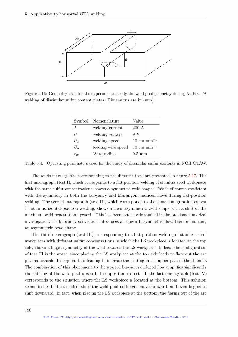
5. Application to horizontal GTA welding
8
6
50
200
124
Figure 5.16: Geometry used for the experimental study the weld pool geometry during NGH-GTA
welding of dissimilar sulfur content plates. Dimensions are in (mm).
Symbol Nomenclature Value
I welding current 200 A
U welding voltage 9 V
Us welding speed 10 cm min−1
Uw feeding wire speed 70 cm min−1
rw Wire radius 0.5 mm
Table 5.4: Operating parameters used for the study of dissimilar sulfur contents in NGH-GTAW.
The welds macrographs corresponding to the different tests are presented in figure 5.17. The
first macrograph (test I), which corresponds to a flat-position welding of stainless steel workpieces
with the same sulfur concentrations, shows a symmetric weld shape. This is of course consistent
with the symmetry in both the buoyancy and Marangoni induced flows during flat-position
welding. The second macrograph (test II), which corresponds to the same configuration as test
I but in horizontal-position welding, shows a clear asymmetric weld shape with a shift of the
maximum weld penetration upward . This has been extensively studied in the previous numerical
investigation; the buoyancy convection introduces an upward asymmetric flow, thereby inducing
an asymmetric bead shape.
The third macrograph (test III), corresponding to a flat-position welding of stainless steel
workpieces with different sulfur concentrations in which the LS workpiece is located at the top
side, shows a huge asymmetry of the weld towards the LS workpiece. Indeed, the configuration
of test III is the worst, since placing the LS workpiece at the top side leads to flare out the arc
plasma towards this region, thus leading to increase the heating in the upper part of the chamfer.
The combination of this phenomena to the upward buoyancy-induced flow amplifies significantly
the shifting of the weld pool upward. In opposition to test III, the last macrograph (test IV)
corresponds to the situation where the LS workpiece is located at the bottom. This solution
seems to be the best choice, since the weld pool no longer moves upward, and even begins to
shift downward. In fact, when placing the LS workpiece at the bottom, the flaring out of the arc
186
PhD Thesis: ”Multiphysics modelling and numerical simulation of GTA weld pools” - Abderrazak Traidia - 2011

5.4. Conclusion
towards the bottom part of the chamfer leads to increase the heat input in this region. As a
consequence, this counterbalances the effect of upward buoyancy-induced flow and leads to limit
the asymmetry observed on test II.
It should be noted that the latter result is to be considered with cautiousness, since the
results of this investigation are conducted only for the first pass. Indeed, one needs to conduct a
multi-pass welding investigation, in order to average out the experimental results before final
conclusion.
2mm5 : 1
2m
m5
: 1
2m
m5
: 1
2m
m5 : 1
LS LS
LS
LS
LS
LSHS
HS
g
g
gg
I
II
IIIIV
2m
m
Figure 5.17: Welds macrographs for the different studied tests.
5.4 Conclusion
An experimental and numerical analysis of horizontal-position welding of stainless steel plates
has been presented in this chapter.
Experimentally, the cross-sections macrographs show a huge asymmetry of the weld about
the plate joint, and a shifting of the maximum weld penetration towards the opposite gravity
PhD Thesis: ”Multiphysics modelling and numerical simulation of GTA weld pools” - Abderrazak Traidia - 2011
187

5. Application to horizontal GTA welding
direction. Additionally, the temperature field distribution at the reverse side of the plate is found
to be slightly affected by the change in the welding position.
Concerning the numerical side, the hybrid 2D-3D model developed in the previous chapter
has been improved to include the effects of gravity on the free surface deformation in horizontal
welding. The computed results confirm the experimental observations, i.e, a huge asymmetry
in the weld shape is observed, especially for high values of welding currents, which induces a
shifting in the location of the maximum weld penetrations towards the opposite gravity direction.
The analysis of the fluid flow directions and the free surface shape shows that the asymmetry of
the weld is attributed to both the upward buoyancy-induced flows and the asymmetry in the
deformation of the weld pool free surface.
Some numerical simulations performed on chamfered geometries confirms the results obtained
for plates simulations and are consistent with the experimental observations identified in the
nuclear industry for NGH-GTAW; i.e., the lateral penetration of the weld is larger in the upper
chamfer than in the bottom one. This makes it possible to reach our final objective, since the
factors (or at least some of them) that are responsible for the asymmetry in the weld shape have
been numerically identified.
Also, a brief experimental study has been conducted to investigate horizontal GTA welding
of stainless steel plates with different concentrations of sulfur. The results show that the weld
asymmetry is considerably reduced when the lowest sulfur content plate is located at the bottom
side. The literature review provides an understanding of this experimental finding; during GTA
welding of stainless steel plates with dissimilar sulfur concentrations, the arc flares out of towards
the low sulfur plate, involving a movement of the cathode spot on the surface of the low sulfur
side away from the high sulfur side. As a consequence the weld is considerably shifted towards
the low sulfur plate.
188
PhD Thesis: ”Multiphysics modelling and numerical simulation of GTA weld pools” - Abderrazak Traidia - 2011

Conclusions and future work
Conclusions
During the assembly of nuclear power plants components using Narrow-Gap Welding technique
with horizontal welding position, an asymmetry in the weld shape has been identified. Indeed,
the lateral penetration of the weld in the upper component was larger than that in the bottom
one. Although many experimental tests, conducted by welding engineers, permitted to reduce
this defect by adjusting the welding parameters, up to the present no answers were given about
the origins of this defect. Then the numerical simulation has become the main alternative.
The purpose of the present work was on the mathematical modelling and numerical simulation
of the weld pool development for both stationary and moving torch GTAW. The main objective
is to build a predictive three-dimensional weld pool model accounting for the filler metal and
welding position. The final aim is to simulate the Narrow-Gap Horizontal-position GTAW process
in order to identify the sources of asymmetries observed experimentally in the nuclear industry.
As welding operations are generally conducted in pulsed current mode and using gas mixtures,
we also aim to quantify the impact of welding parameters on the resulting weld shapes.
The first part of this work focused on the field of modelling and numerical simulation of spot
GTA welding. First, using a transient 2D weld pool model, presented in the second chapter,
we numerically studied GTA weld pools developments for pulsed current welding. The results
revealed the appearing of two vortices in the weld pool: a counter-clockwise vortex near the weld
axis and a clockwise vortex near the edges of the pool boundary. These two vortices which are
closely linked to the change in the sign of the surface tension gradient, evolved with time and
dominated cyclically each other during the whole welding process. This phenomenon that we
called ’alternate domination of vortices’ explained an interesting finding: the weld pool width and
depth evolved in the opposite directions; i.e., the weld width increased during peak time while
the depth decreased, however during the background time, the width decreased while the depth
increased. The results emphasized the importance of considering a surface tension coefficient
variable with both temperature and sulfur activity, rather than assuming an arbitrary constant
value.
The model was also used to investigate the choice of welding parameters in pulsed current
welding. The weld pool dimensions were found to be larger when the gap between the peak and
background current is important, and for the lowest welding frequency. At constant welding
PhD Thesis: ”Multiphysics modelling and numerical simulation of GTA weld pools” - Abderrazak Traidia - 2011
189

Conclusions and future work
energy, the peak pulse duration was found to have much less influence on the weld pool dimensions
than the current ratio and pulse frequency. Additionally, we found that pulsed current welding
produced a larger and deeper weld than the corresponding mean current, which underlined the
benefits of pulsed current mode, and suggested that pulsed current welds cannot be approximated
by the corresponding mean current welds. The model was also applied to study a virtual
axisymmetric heating of a thick pipe with a narrow groove, and the computed results showed a
huge asymmetry of the weld about the center line. This was numerically found to be caused by
the upward buoyancy-induced flow, convecting hot fluid toward the opposite gravity direction,
and represented an important step toward explaining the asymmetry of lateral penetrations in
NGH-GTAW.
The comparison between different models showed that for welding currents below 200 A,
a weld pool model assuming a ’flat’ free surface is highly recommended, as the free surface
depression is negligible compared to the weld dimensions. For higher values of welding currents, a
self-consistent calculation of the free surface deformation is needed to get more predictive results.
To improve the model predictivity, we introduced in the third chapter a coupled arc/weld-pool
model, in which the heat transfer, fluid flow and electromagnetic fields were solved in the three
regions of the process, accounting for the discontinuities at the arc-electrodes interfaces. After
validating the model results on some studies available in the literature, we showed that the
heat flux and current density at the anode stabilised very quickly after the arc ignition (in
approximately 15 ms) which means that the energy transferred to the anode during pulsed
current mode can be reasonably approximated by a cyclic variation between the two constant
steady-state solutions corresponding respectively to the peak and background currents. Real-time
observation of the weld pool was realised using an Infrared camera, which made it possible to
validate the model results and pointed out the main limit of our model which is the absence of
metal vapours.
The model also permitted a numerical investigation of the effect of helium addition on the
heat transfer and fluid flow during GTA welding. The computed results showed that the plasma
temperature, gas velocity, anodic heat flux and current densities, as well as the total energy
transferred to the workpiece increased considerably with helium mole fraction in the mixture.
This necessarily increased the governing forces in the weld pool leading to increase the weld
pool dimensions. In addition, an electromagnetically-induced vortex was identified for high
helium mole fractions, leading to amplify the weld pool penetration by a factor of up to 3.
Unexpectedly, we found that the presence of a small amount of argon (as low as 10 %) in the gas
mixture, decreased considerably the heat flux and then the weld penetration, which is due to the
thermophysical properties of argon-helium mixtures that are highly modified by the presence of
any amount of argon. The comparison with the welds macrographs showed a good agreement,
but also highlighted the importance of accounting for the metal vapours, especially for pure
helium arcs where the process efficiency would be considerably decreased.
As the developed coupled arc/weld-pool model is time-dependent, it also permitted the study
190
PhD Thesis: ”Multiphysics modelling and numerical simulation of GTA weld pools” - Abderrazak Traidia - 2011

Conclusions and future work
of a new GTA welding technique called ’the alternate supply of shielding gases’. The computed
results showed that the electromagnetically induced vortex appears during helium supply and
disappears during argon supply. This gas supplying technique produced the same effects as a
pure helium arc, with less helium use, and with less energy transferred to the workpiece. This
new technique is not used in industrial applications yet, but would be cost saving, and would
limit considerably residual distortions after cooling.
The second part of this work was devoted to study moving GTAW with filler metal. A
preliminary experimental analysis showed that the feeding wire had nearly no influence on the
measured thermal cycles at the reverse side of the workpiece, whereas it significantly affected
the weld shape by decreasing the weld penetration. This finding has been attributed to the
absorption of energy by the feeding wire from the hot molten pool.
A hybrid 2D-3D approach has been introduced in the fourth chapter to numerically simulate
moving GTA weld pools. The boundary conditions at the workpiece surface were 2D-computed
using the arc plasma model developed in the third chapter, whereas the steady-state weld shape
was computed using a 3D weld pool model. The latter included a two-ways coupling with the
free surface deformation and accounted for the filler metal effects on the energy and momentum
balances. In the presence of filler metal, the numerical results showed that the weld depth was
locally decreased in the region thermally affected by the feeding wire, especially for low current
welds. The comparison with the experimental measurements showed that, despite the use of a 2D
model for the determination of the boundary conditions at the workpiece surface, the weld shapes,
maximum temperatures reached and thermal cycles were relatively well predicted. However, the
numerical results overestimated the cooling rates at the rear of the welding electrode, which has
been numerically found to be linked to the value chosen for the anode emissivity.
Horizontal-position welding has been investigated in the last chapter both experimentally
and numerically. The cross-section macrographs showed a huge asymmetry of the weld about
the plate joint, and a shifting of the maximum weld penetration towards the opposite gravity
direction. The hybrid 2D-3D model developed in the fourth chapter has been improved to
include the effects of gravity on the free surface deformation in horizontal welding. The computed
results confirmed the experimental observations. The analysis of the fluid flow directions and the
free surface shape revealed that the asymmetry of the weld was the result of both the upward
buoyancy-induced flows and the asymmetry in the deformation of the weld pool free surface.
Some numerical simulations performed on chamfered geometries showed a good agreement
with the experimental observations identified in the nuclear industry for NGH-GTAW; i.e., the
lateral penetration of the weld is larger in the upper chamfer than in the bottom one. Additionally,
the weld asymmetry was found to be more important for high values of welding current. These
numerical results allowed us to reach our final objective, since the factors (or at least some of
them) that are responsible for the asymmetry in the weld shape have been numerically identified
in the fourth chapter.
As an extension, a brief experimental study has been conducted to investigate horizontal
PhD Thesis: ”Multiphysics modelling and numerical simulation of GTA weld pools” - Abderrazak Traidia - 2011
191

Conclusions and future work
GTA welding of stainless steel plates with different concentrations of sulfur. The results showed
that the weld asymmetry could be considerably reduced when the lowest sulfur content plate was
located at the bottom side. The literature review provided an explanation to this experimental
finding; the arc flared out towards the low sulfur plate because of manganese metal vapours
present in this region. This involved a movement of the cathode spot on the surface of the low
sulfur side away from the high sulfur side and consequently the weld was considerably shifted
towards the low sulfur chamfer.
Future work
The results of the present work motivated us to raise new challenges. The experimental and
numerical prospectives recommended for the future are as follows:
• A rigorous experimental study should be conducted for a better estimation of the surface
tension coefficient for stainless steel materials. This also includes the determination of
the standard heat of adsorption ∆H0 for AISI 304 accounting for all the surface active
elements present in this alloy.
• Great efforts should be made on the imaging aspect. In particular, real-time observations
of the weld pool behaviour during the immersion, melting and wetting of the feeding wire
would not only lead to a better understanding of the physical phenomena behind the
resultant weld defects, but also to an improvement of the current numerical weld pool
models.
• The alternate supply of shielding gases introduced in the third chapter should be experimen-
tally analysed with different operating parameters. It would be very interesting to study
this new welding technique with various supplying frequencies, and inflow rate ratios, so as
to optimize the choice of these parameters to get the best weld quality. Additionally, it
should be mentioned that this method is currently being investigated by Korean researchers
on Narrow-Gap welding applications for the nuclear industry.
• As concerns the two-dimensional models developed in this study, we should mention the
absence of the influence of metal vapours in our models. This weakness can be quite
important, especially for high welding currents or when using pure helium as a shielding
gas. The future developments should account for this effect, which requires including the
dependence of the shielding gas properties on the fraction of metal vapours (obtained by
solving additional diffusion equations).
• Concerning moving GTA weld pools with filler metal, besides the 2D computation of
the boundary conditions at the workpiece surface that should be reviewed, the main
improvement planed for the near future is to include the feeding wire in the computational
domain and to deal with the whole problem in a unified formalism.
192
PhD Thesis: ”Multiphysics modelling and numerical simulation of GTA weld pools” - Abderrazak Traidia - 2011

Conclusions and future work
• A multiphysics-based approach for the determination of residual stresses and distortions
after cooling can be conceivable (at least for stationary GTAW). This can be done by
coupling the HFF and TMM approaches. It would make possible understanding the impact
of the fluid flow in the weld pool on the residual state of the welded joint, but would also
improve the predictions since the gas composition, the electrode shape and the arc-length
are directly included in the computational domain.
PhD Thesis: ”Multiphysics modelling and numerical simulation of GTA weld pools” - Abderrazak Traidia - 2011
193

Conclusions and future work
194
PhD Thesis: ”Multiphysics modelling and numerical simulation of GTA weld pools” - Abderrazak Traidia - 2011

Bibliography
[1] M. Brochard. Modele couple cathode-plasma-piece en vue de la simulation du procede de
soudage a l’arc TIG. PhD thesis, Ecole Polytechnique Universitaire de Marseille (France),
2009.
[2] J. Scemeliovas. Determination of pulse current optimal parameters for manualarc welding.
Mechanika, 51:66–69, 2005.
[3] T. Mohandas and GM. Reddy. A comparison of continuous and pulse current gas tungsten
are welds of an ultra high strength steel. Journal of Materials Processing Technology, 69:
222–226, 1997.
[4] E. Pfender. Electric arcs and arc gas heaters. Gaseous Electronics, 1:291–398, 1978.
[5] I.M. Richardson. Arc Welding and Hybrid Laser-Arc Welding, volume 10, chapter 6 of The
Theory of Laser Materials Processing. Springer edition, 2009.
[6] M. Tanaka and JJ. Lowke. Predictions of weld pool profiles using plasma physics. Journal
of Physics D-Applied Physics, 40:R1–R23, 2007.
[7] JF. Lancaster. The Physics of Welding. Pergamon Press, 1986.
[8] S. Mishra, TJ. Lienert, MQ. Johnson, and T. DebRoy. An experimental and theoretical
study of gas tungsten arc welding of stainless steel plates with different sulfur concentrations.
Acta Materialia, 56:2133–2146, 2008.
[9] PC. Zhao, CS. Wu1, and ZM. Zhang. Modelling the transient behaviours of a fully penetrated
gas–tungsten arc. Proc. IMechE Vol. 219 Part B: J. Engineering Manufacture, 2005.
[10] T. Zacharia, SA. David, JM. Vitek, and T. DebRoy. Weld pool development during GTA
and laser-beam welding of type-304 stainless steel .1. theoretical-analysis. Welding Journal,
68(12):–499, DEC 1989.
[11] DK. Aidun and SA. Martin. Effect of sulfur and oxygen on weld penetration of high-purity
austenitic stainless steels. Journal of Materials Engineering and Performance, 6:496–502,
1997.
[12] WH. Kim and SJ. Na. Heat and fluid flow in pulsed current GTA weld pool. International
Journal of Heat and Mass Transfer, 41:3213–3227, 1998.
PhD Thesis: ”Multiphysics modelling and numerical simulation of GTA weld pools” - Abderrazak Traidia - 2011
195

Bibliography
[13] Z. Yang and T. DebRoy. Modeling macro-and microstructures of gas-metal-arc welded
hsla-100 steel. Metallurgical and Materials Transactions B-Process Metallurgy and Materials
Processing Science, 30:483–493, 1999.
[14] N. Chakraborty and S. Chakraborty. Influences of sign of surface tension coefficient on
turbulent weld pool convection in a gas tungsten arc welding (GTAW) process: A comparative
study. Journal of Heat Transfer-Transactions of the ASME, 127:848–862, 2005.
[15] M. Tanaka and JJ. Lowke. An introduction to physical phenomena in arc welding processes.
Welding International, 18:11, 2004.
[16] M. Tanaka, H. Terasaki, and M. Ushio. Numerical study of weld formation for stationary
TIG arc in different gaseous atmosphere. Annual Assembly of the IIW, Doc. 212-1040-03,
2003.
[17] AB. Murphy, M. Tanaka, S. Tashiro, T. Sato, and JJ. Lowke. A computational investigation
of the effectiveness of different shielding gas mixtures for arc welding. Journal of Physics
D-Applied Physics, 42:115205, 2009.
[18] RTC. Choo and J. Szekely. Vaporization kinetics and surface-temperature in a mutually
coupled spot gas tungsten arc weld and weld pool - thermocapillary flow proves to be an
important factor in governing free-surface temperature distribution. Welding Journal, 71(3):
77, 1992.
[19] P. Sahoo, T. DebRoy, and MJ. McNallan. Surface-tension of binary metal - surface-active
solute systems under conditions relevant to welding metallurgy. Metallurgical Transactions
B-Process Metallurgy, 19:483–491, 1988.
[20] HG. Fan, HL. Tsai, and SJ. Na. Heat transfer and fluid flow in a partially or fully penetrated
weld pool in gas tungsten arc welding. International Journal of Heat and Mass Transfer, 44:
417–428, 2001.
[21] J. Hu, H. Guo, and HL. Tsai. Weld pool dynamics and the formation of ripples in 3D gas
metal arc welding. International Journal of Heat and Mass Transfer, 51:2537–2552, 2008.
[22] W. Zhang. Fluid flow and microstructure evolution during fusion welding of alloys. PhD
thesis, The Pennsylvania State University, USA, 2005.
[23] CX. Zhao. Measurements of fluid flow in weld pools. PhD thesis, Delft University of
Technology, Delft, Netherlands, 2011.
[24] M. Hamide. Modelisation numerique du soudage a l’arc des aciers. PhD thesis, Mines-
ParisTech, France, 2008.
[25] SP. Lu, WC. Dong, DZ. Li, and YY. Li. Numerical study and comparisons of gas tungsten
arc properties between argon and nitrogen. Computational Materials Science, 45:327–335,
2009. doi: 10.1016/j.commatsci.2008.10.010.
196
PhD Thesis: ”Multiphysics modelling and numerical simulation of GTA weld pools” - Abderrazak Traidia - 2011

Bibliography
[26] KC. Hsu, K. Etemadi, and E. Pfender. Study of the free burning high intensity argon arc.
Journal of Applied Physics, 54(3):1293–1301, 1983.
[27] J. Mckelliget and J. Szekely. Heat-transfer and fluid-flow in the welding arc. Metallurgical
Transactions A-Physical Metallurgy and Materials Science, 17:1139–1148, 1986.
[28] HG. Fan and YW. Shi. Numerical simulation of the arc pressure in gas tungsten arc welding.
Journal of Materials Processing Technology, 61:302–308, 1996.
[29] HG. Fan, YW. Shi, and SJ. Na. Numerical analysis of the arc in pulsed current gas tungsten
arc welding using a boundary-fitted coordinate. Journal Of Materials Processing Technology,
72:437–445, 1997.
[30] M. Goodarzi, R. Choo, and JM. Toguri. The effect of the cathode tip angle on the GTAW
arc and weld pool .1. mathematical model of the arc. Journal of Physics D: Applied Physics,
30(19):2744–2756, 1997.
[31] M. Goodarzi, R. Choo, T. Takasu, and JM. Toguri. The effect of the cathode tip angle on
the gas tungsten arc welding arc and weld pool: Ii. the mathematical model for the weld
pool. Journal of Physics D: Applied Physics, 31(5):569–583, 1998.
[32] L. Sansonnens, J. Haidar, and JJ. Lowke. Prediction of properties of free burning arcs
including effects of ambipolar diffusion. Journal of Physics D-Applied Physics, 33:148–157,
2000.
[33] CS. Wu and JQ. Gao. Analysis of the heat flux distribution at the anode of a TIG welding
arc. Computational Materials Science, 24:323–327, 2002.
[34] HY. Du, YH. Wei, WX. Wang, WM. Lin, and D. Fan. Numerical simulation of temperature
and fluid in GTAW-arc under changing process conditions. Journal of Materials Processing
Technology, 209:3752–3765, 2009.
[35] HR. Saedi and Unkel W. . Arc weld pool behavior for pulsed current GTAW. Weld. J, Res.
Suppl., pages 247–255, 1988.
[36] M. Kanouff and R. Greif. The unsteady development of a GTA weld pool. International
Journal of Heat and Mass Transfer, 35(4):967–979, 1992.
[37] CS. Wu and L. Dorn. Computer simulation of fluid dynamics and heat transfer in full-
penetrated TIG weld pools with surface depression. Computational Materials Science, 2(2):
341–349, 1994.
[38] CS. Wu, W. Zheng, and L. Wu. Modelling the transient behaviour of pulsed current tungsten-
inert-gas weldpools. Modelling and Simulation in Materials Science and Engineering, 7(1):
15, 1999.
PhD Thesis: ”Multiphysics modelling and numerical simulation of GTA weld pools” - Abderrazak Traidia - 2011
197

Bibliography
[39] SH. Ko, DF. Farson, SK. Choi, and CD. Yoo. Mathematical modeling of the dynamic
behavior of gas tungsten arc weld pools. Metallurgical and Materials Transactions B-Process
Metallurgy and Materials Processing Science, 31:1465–1473, 2000.
[40] T. DebRoy and DeHerrera. Computer calculations of fusion zone geometry considering fuid
fow and heat transfer during fusion welding. Technical report, The University of Texas at
El Paso, 2002.
[41] W. Zhang, GG. Roy, JW. Elmer, and T. DebRoy. Modeling of heat transfer and fluid flow
during gas tungsten arc spot welding of low carbon steel. Journal of Applied Physics, 93:
3022–3033, 2003. doi: 10.1063/1.1540744.
[42] F. Roger and K. Dang Van. Prediction of the weld shape in arc welding, a numerical
modeling example in multiphysics coupling. Revue Europeenne des elements finis, 13:5–7,
2004.
[43] CS. Wu, PC. Zhao, and YM. Zhang. Numerical simulation of transient 3-D surface deforma-
tion of a completely penetrated GTA weld - an analytical model that explores the dynamic
behavior of a weld pool will help in the development of a sensor that detects complete joint
penetration in gas tungsten arc welding. Welding Journal, 83:330S–335S, 2004.
[44] CS. Wu, J. Chen, and YM. Zhang. Numerical analysis of both front- and back-side
deformation of fully-penetrated GTAW weld pool surfaces. Computational Materials Science,
39:635–642, 2007.
[45] A. Kumar and T. DebRoy. Calculation of three-dimensional electromagnetic force field
during arc welding. Journal of Applied Physics, 94:1267–1277, 2003. doi: 10.1063/1.1587006.
[46] M. Tanaka, H. Terasaki, M. Ushio, and JJ. Lowke. A unified numerical modeling of stationary
tungsten-inert-gas welding process. Metallurgical and Materials Transactions A-Physical
Metallurgy and Materials Science, 33:2043–2052, 2002.
[47] M. Tanaka, H. Terasaki, M. Ushio, and JJ. Lowke. Numerical study of a free-burning argon
arc with anode melting. Plasma Chemistry and Plasma Processing, 23:585–606, 2003.
[48] FG. Lu, S. Yao, SN. Lou, and YB. Li. Modeling and finite element analysis on GTAW arc
and weld pool. Computational Materials Science, 29:371–378, 2004.
[49] FG. Lu, XH. Tang, HL. Yu, and S. Yao. Numerical simulation on interaction between TIG
welding arc and weld pool. Computational Materials Science, 35:458–465, 2006.
[50] JJ. Lowke and M. Tanaka. ’lte-diffusion approximation’ for arc calculations. Journal of
Physics D-Applied Physics, 39:3634–3643, 2006.
[51] S. Tashiro and M. Tanaka. Numerical study of tube cathode arc with anode melting. Robotic
Welding, Intelligence and Automation, 362:127–134, 2007.
198
PhD Thesis: ”Multiphysics modelling and numerical simulation of GTA weld pools” - Abderrazak Traidia - 2011

Bibliography
[52] AB. Murphy, M. Tanaka, K. Yamamoto, S. Tashiro, JJ. Lowke, and Ostrikov K. Modelling
of arc welding: The importance of including the arc plasma in the computational domain.
Vacuum, 85:579–584, 2010.
[53] AB. Murphy, M. Tanaka, K. Yamamoto, S. Tashiro, T. Sato, and JJ. Lowke. Modelling
of thermal plasmas for arc welding: the role of the shielding gas properties and of metal
vapour. Journal of Physics D-Applied Physics, 42:194006, 2009.
[54] F. Lago, JJ. Gonzalez, P. Freton, and A. Gleizes. A numerical modelling of an electric arc
and its interaction with the anode: Part 1. the two-dimensional model. Journal of Physics
D-Applied Physics, 37:883–897, 2004.
[55] F. Lago, JJ. Gonzalez, P. Freton, F. Uhlig, N. Lucius, and GP. Piau. A numerical modelling
of an electric arc and its interaction with the anode: part iii. application to the interaction
of a lightning strike and an aircraft in flight. Journal of Physics D-Applied Physics, 39:
2294–2310, 2006.
[56] JJ. Gonzalez, F. Lago, P. Freton, M. Masquere, and X. Franceries. Numerical modelling
of an electric arc and its interaction with the anode: part ii. the three-dimensional model -
influence of external forces on the arc column. Journal of Physics D-Applied Physics, 38(2):
306–318, 2005.
[57] G. Xu, J. Hu, and HL. Tsai. Three-dimensional modeling of the plasma arc in arc welding.
Journal Of Applied Physics, 104:103301, 2008.
[58] G. Xu, J. Hu, and HL. Tsai. Three-dimensional modeling of arc plasma and metal transfer
in gas metal arc welding. International Journal of Heat and Mass Transfer, 52:1709–1724,
2009.
[59] E. Friedman. Thermomechanical analysis of the welding process using the finite element
method. Journal of Pressure Vessel Technology, 97:206–213, 1975.
[60] JM. Bergheau. Modelisation numerique des procedes de soudage. Technical report, Tech-
niques de l’Ingenieur, BM7758, 2004.
[61] K. Runesson, A. Skyttebol, and LE. Lindgren. Nonlinear finite element analysis and
application to welded structures. Numerical and Computational Methods, B. Karihaloo,
Elsevier, 3:255–320, 2003.
[62] PR. Vishnu, WB. Li, and KE. Easterling. Heat fluid model for pulsed welding. Materials
Science and Technology, 7:649–659, 1991.
[63] M. Ushio and CS. Wu. Mathematical modeling of three-dimensional heat and fluid flow
in a moving gas metal arc weld pool. Metallurgical and Materials Transactions B-Process
Metallurgy and Materials Processing Science, 28:509–516, 1997.
PhD Thesis: ”Multiphysics modelling and numerical simulation of GTA weld pools” - Abderrazak Traidia - 2011
199

Bibliography
[64] A. D. Brent, V. R. Voller, and Reid KJ. Enthalpy-porosity technique for modeling convection-
diffusion phase change: application to the melting of a pure metal. Numerical Heat Transfer,
13:297–318, 1988.
[65] M. Carin and E. Favre. Numerical simulation of fluid flow during arc welding. In COMSOL
Multiphysics User’s Conference. Paris 2005, 2005.
[66] C. Delalondre. Modelisation aerodynamique d’arcs electriques a fortes intensite avec prise
en compte du desequilibre thermodynamique local et du transfert thermique a la cathode.
PhD thesis, Universite de Rouen, France, 1990.
[67] J. J. Lowke. Simple theory of free-burning arcs. Journal of Physics D: Applied Physics, 12:
1873–1886, 1979.
[68] M. Ushio, D. Fan, and M. Tanaka. Trans. JWRI 22, pages 201–207, 1993.
[69] JJ. Lowke, R. Morrow, and J. Haidar. A simplified unified theory of arcs and their electrodes.
Journal of Physics D: Applied Physics, 30(14):2033, 1997.
[70] M. Boulos, P. Fauchais, and E. Pfender. Thermal plasma, fundamentals and applications.
Plenum Press, 1994.
[71] X. Zhou and J. Heberlein. An experimental investigation of factors affecting arc-cathode
erosion. Journal of Physics D: Applied Physics, 31(19):2577, 1998.
[72] M. Marya, G.R. Edwards, and S. Liu. An investigation on the effects of gases in GTA
welding of a wrought az80 magnesium alloy. Welding Journal, 83:203s–212s, 2004.
[73] M. Onsoien, R. Peters, D.L. Olson, and S. Liu. Effect of hydrogen in an argon GTAW
shielding gas: arc characteristics and bead morphology. Welding Journal, 74:10s–15s, 1995.
[74] J. Tusek. Experimental investigation of gas tungsten arc welding and comparison with
theoretical predictions. Plasma Science, IEEE Transactions on, 2000.
[75] OM. Novikov. Russian Patent N. 2008153, 1992.
[76] S.C. Woods. Investigation of the effect of pulsing shielding gas in arc welding. Master’s
thesis, College of Engineering. The Ohio State University, 2006.
[77] BY. Kang, YKDV. Prasad, MJ. Kang, HJ. Kim, and IS. Kim. The effect of alternate supply
of shielding gases in austenite stainless steel GTA welding. Journal of Materials Processing
Technology, 209:4722–4727, 2009.
[78] Kim IS., JS. Son, HG. Kim, and BA. Chin. Development of a mathematical model to study
on variation of shielding gas in GTA welding. Journal of Achievements in Materials and
Manufacturing Engineering, 19(2):73–80, 2006.
200
PhD Thesis: ”Multiphysics modelling and numerical simulation of GTA weld pools” - Abderrazak Traidia - 2011

Bibliography
[79] J. Goldak, M. Bibby, J. Moore, R. House, and B. Patel. Computer modeling of heat-flow in
welds. Metallurgical Transactions B-Process Metallurgy, 17(3):587–600, 1986.
[80] S. Bag, A. Trivedi, and A. De. Development of a finite element based heat transfer model
for conduction mode laser spot welding process using an adaptive volumetric heat source.
International Journal of Thermal Sciences, 48(10):1923 – 1931, 2009.
[81] YS. Touloukian. Thermophysical properties of high temperature solid materials, volume 3.
The macmillan co. edition, 1967.
[82] S. Tashiro. Plasma properties for helium gas tungsten arc with metal vapor. J. JapanWelding
Soc., 24-2:143–148, 2006.
[83] CS. Wu and KC. Tsao. Modelling the three-dimensional fluid flow and heat transfer in a
moving weld pool. Engineering Computational, 7:241–248, 1990.
[84] H. G. Fan and R. Kovacevic. Three-dimensional model for gas tungsten arc welding with
filler metal. Proceedings of the Institution of Mechanical Engineers Part B, 220(7):1107–1115,
2006.
[85] E. Le Guen. Etude du procede de soudage hybride laser/MAG: Caracterisation de la geometrie
et de l’hydrodynamique du bain de fusion et developpement d’un modele 3D thermique. PhD
thesis, Universite de Bretagne Sud, France, 2010.
[86] C. L. Yang, N. Guo, S. B. Lin, C. L. Fan, and Y. Q. Zhang. Application of rotating arc
system to horizontal narrow gap welding. Science and Technology of Welding and Joining,
14(2):172–177, 2009.
[87] Jiayou Wang, Jie Zhu, Ping Fu, Rongjin Su, Wei Han, and Feng Yang. A swing arc system
for narrow gap GMA welding. ISIJ International, 52(1):110–114, 2012.
[88] WC. Bennett and GS. Mills. Welding Journal, 53:548s, 1974.
[89] RTC. Choo and J. Szekely. Possible role of turbulence in GTA weld pool behaviour. Welding
Journal, 73(2):25s–31s, 1994.
[90] CW. Hirt and BD. Nichols. Volume of fluid (vof) method for the dynamics of free boundaries.
Journal of Computational Physics, 39:210, 1981.
[91] D. Delapp, G. Cook, A. Strauss, and W. Hofmeister. Quantitative observations of surface
flow and solidification on autogeneous GTA weld pools. In ASM Proceedings of international
conference, Trends in Welding Research, 2005.
[92] D. Delapp. Observations of solidification and surface flow on autogeneous tungsten arc weld
pools. PhD thesis, Vanderbilt University, Nashville, Tennessee, USA.
[93] DR. Atthey. A mathematical model for fluid flow in a weld pool at high currents. Journal
of Fluid Mechanics, 98(4):787–801, 1980.
PhD Thesis: ”Multiphysics modelling and numerical simulation of GTA weld pools” - Abderrazak Traidia - 2011
201

Bibliography
[94] GM. Oreper, TW. Eagar, and J. Szekely. Convection in arc weld pools. Welding Journal,
62:307s–312s, 1983.
[95] S. Kou and YH. Wang. Three-dimensional convection in laser melted pools. Materials
Transactions A, 17A:2265–2270, 1985.
[96] S. Kou and YH. Wang. Fluid-flow and weld penetration in stationary arc welds. Materials
Transactions A, 16A(2):203–213, 1985.
[97] J. Jaidi and P. Dutta. Three-dimensional turbulent weld pool convection in gas metal arc
welding process. Science and Technology of Welding and Joining, 9(5):407–414, 2004.
[98] C. Winkler, H. Amberg, H. Inoue, and T. Koseki. A numerical and experimental investigation
of qualitatively different weld pool shapes. Mathematical modelling of weld phenomena, 4:
37–69, 1984.
[99] J. Donea, A. Huerta, J.Ph. Ponthot, and A. Rodriguez-Ferran. Arbitrary Lagrangian-Eulerian
Methods, Chapter 14, volume I. Encyclopedia of computational mechanics edition, 2004.
202
PhD Thesis: ”Multiphysics modelling and numerical simulation of GTA weld pools” - Abderrazak Traidia - 2011

Appendix A:
Reynolds number during welding
Up to the present, it is still unclear whether the molten metal flow during welding is laminar
or turbulent. Recently, Zhao [23] proposed a summary of reported Reynolds numbers during
welding, as presented in Table 5.5. Most of the numerical models assume laminar flow, since
this assumption permit to get quite good results with reduced computing times. However, visual
observations of the weld pool indicate unsteady chaotic behaviour, traducing a certain transition
from laminar to turbulent flows [89]. To be more rigorous, depending on welding conditions, the
molten metal flow may not be fully laminar.
Method Year Re Vmax (m s−1) Material Result
Exp [90] 1990 3000 0.5 AISI310 Turbulent
Exp [91, 92] 2005 107 0.0346 Carbon steel
Num [93] 1980 200-600 0.105 Laminar
Num [94] 1983 2000-3000 1.259 Carbon steel Laminar
Num [95] 1985 1300 3 AA6061 Laminar
Num [96] 1985 1400 0.25 AISI304 Laminar
Num [89] 1994 4700 0.7 AISI304 Turbulent
Num [97] 2004 3000 0.08 Steel Turbulent
Num [98] 1998 11000 1.22 Type304 Turbulent
Table 5.5: A summary of reported Reynolds numbers during welding [23].
PhD Thesis: ”Multiphysics modelling and numerical simulation of GTA weld pools” - Abderrazak Traidia - 2011
203

Appendix A:Reynolds number during welding
204
PhD Thesis: ”Multiphysics modelling and numerical simulation of GTA weld pools” - Abderrazak Traidia - 2011

Appendix B:
A brief review of the ALE method
The principle
In continuum mechanics, we usually make use of two classical descriptions of motion: the
Lagrangian description and the Eulerian description. Because of the drawbacks of purely
Lagrangian and purely Eulerian descriptions, a technique has been developed that succeeds
in combining the best features of both the Lagrangian and the Eulerian approaches. Such a
technique is known as the Arbitrary Lagrangian Eulerian (ALE) description.
Figure 5.18: Particles and meshes motion during Lagrangian, Eulerian, and ALE motion
descriptions [99].
In the ALE description, the nodes of the computational mesh may be moved with the
continuum in normal Lagrangian fashion, or be held fixed in Eulerian manner, or, as shown in
Figure 5.18, be moved in some arbitrarily specified way (for example to capture the location of
PhD Thesis: ”Multiphysics modelling and numerical simulation of GTA weld pools” - Abderrazak Traidia - 2011
205

Appendix B:A brief review of the ALE method
the a free surface). Because of this freedom in moving the computational mesh offered by the
ALE description, the mesh distortions encountered when using a purely Lagrangian method are
handled, with more flexibility than that offered by a purely Eulerian description.
ALE form of the classical conservation equations
In the ALE description of motion, neither the material framework, nor the spatial framework is
taken as the reference. Thus, a third framework is needed for the description of motion, which
is the ALE framework where new ALE coordinates χ are introduced to identify the mesh grid
points.
All one has to do to obtain the ALE form of the classical conservation equations, is to take
the equations written in pure Eulerian description, and to replace in the various convective terms,
the material velocity ~v with the new ALE convective velocity ~c = ~v − ~v, as follows [99]:
∂ρ
∂t|χ +∇ · (ρ~c) = 0
ρ
(∂~v
∂t|χ + ~c · ∇~v
)= ∇ · σ + ~Fv
∂(ρh)
∂t|χ +∇ · (ρh~c) = −∇ · ~q +Qv
(5.12)
Where ~v is material velocity , ~v is mesh velocity, ρ is density, σ is the Cauchy stress tensor, ~Fv is
body forces and h is enthalpy. Note that the classical Lagrangian and Eulerian mesh descriptions
are contained in the above ALE forms. The Lagrangian description corresponds to selecting~v = ~v (~c = ~0), while the Eulerian description corresponds to selecting ~v = ~0 (~c = ~v).
206
PhD Thesis: ”Multiphysics modelling and numerical simulation of GTA weld pools” - Abderrazak Traidia - 2011

Appendix C:
General form of the free surface
deformation model
zy
z=φ(x,y)
O
SL
gz
xO
α1 gx
yO
α2x
Figure 5.19: Schematic representation of the free surface shape and gravity orientation in GTAW.
Initially we assume the gravity vector ~g to be on the z-axis, a first y-axis rotation is denoted α1,
followed by a z-axis rotation denoted α2 . As a result the gravity vector ~g coordinates are given
as follows:
~g =
g cos(α2) sin(α1)
g sin(α2) sin(α1)
g cos(α1)
(x,y,z)
(5.13)
To avoid cumbersome expressions, the cos operator is denoted as c and the sin operator is
denoted as s.
At the equilibrium, the free surface shape z = φ(x, y) minimizes the total energy of surface
Et (which is the sum of the surface deformation energy Ed, the gravitational potential energy Ep
and the arc pressure energy Ea). The expressions of the surface deformation and arc pressure
PhD Thesis: ”Multiphysics modelling and numerical simulation of GTA weld pools” - Abderrazak Traidia - 2011
207

Appendix C:General form of the free surface deformation model
energies are not dependent on the welding position and are still given as follows:
Ed + Ea = Ed −Wa =
∫∫St
γ(√
1 + φ2x + φ2
y − 1)
dxdy −∫∫
St
Parcφ dxdy (5.14)
Where Parc is the arc pressure (positive value) computed using the two-dimensional arc plasma
model.
As concerns the gravitational potential energy Ep of the volume V located under the free
surface, it is computed as follows:
Ep = −∫∫∫
Vρ~g · ~OM dV
= −∫∫∫
Vρ(gcα2sα1~x+ gsα2sα1~y + gcα1~z) · (x~x+ y~y + z~z) dV
= −∫∫∫
Vρg(cα2sα1x+ sα2sα1y + cα1z) dV
= −∫∫
St
[∫ 0
φ(x,y)ρg(cα2sα1x+ sα2sα1y + cα1z) dz
]dxdy
=
∫∫St
ρg(cα2sα1xφ+ sα2sα1yφ+1
2cα1φ
2) dxdy
(5.15)
Then, the total energy of surface Et is expressed as following:
Et = Ed + Ep −Wa
=
∫∫St
γ(√
1 + φ2x + φ2
y − 1)
dxdy +
∫∫St
ρg(cα2sα1xφ+ sα2sα1yφ+1
2cα1φ
2) dxdy
−∫∫
St
Parcφ dxdy
=
∫∫St
F (x, y, φ, φx, φy) dxdy
(5.16)
Accounting for the filler metal leads to verify the following additional constraint (the first
minus sign is due to the descendant orientation of the z-axis):
−∫∫
St
(φ− z0) dxdy =
∫∫St
Gdxdy = ∆Vd (5.17)
Where z0 is the z-location of the initial undeformed free surface.
By applying the Euler-Lagrange criterion, we get:
∂
∂φ(F + λG)− ∂
∂x
[∂
∂φx(F + λG)
]− ∂
∂y
[∂
∂φy(F + λG)
]= 0 (5.18)
Where λ is a Lagrange multiplier introduced to satisfy the conservation equation 5.17.
After manipulation, we obtain the following partial differential equation that governs the free
208
PhD Thesis: ”Multiphysics modelling and numerical simulation of GTA weld pools” - Abderrazak Traidia - 2011

Appendix C:General form of the free surface deformation model
surface shape in horizontal-position welding:
− ∂
∂x
γ φx√1 + φ2
x + φ2y
− ∂
∂y
γ φy√1 + φ2
x + φ2y
+ ρg(cα2sα1x+ sα2sα1y+ cα1φ) = Parc + λ
(5.19)
The above equation can be written in the following usual form:
−γφxx(1 + φ2
x)− 2φxφy + φyy(1 + φ2y)
(1 + φ2x + φ2
y)32
= Parc + λ− ρg(cα2sα1x+ sα2sα1y + cα1φ) (5.20)
The above Partial Differential Equation can be used to compute the free surface shape for
any welding position just by adjusting the values of α1 and α2. In the case of some usual welding
positions, the corresponding PDE’s are as follows:
• Flat-position welding (1g): α1 = 0, α2 = 0
−γφxx(1 + φ2
x)− 2φxφy + φyy(1 + φ2y)
(1 + φ2x + φ2
y)32
= Parc + λ− ρgφ (5.21)
• Horizontal-position welding (2g): α1 = 90, α2 = 90
−γφxx(1 + φ2
x)− 2φxφy + φyy(1 + φ2y)
(1 + φ2x + φ2
y)32
= Parc + λ− ρgy (5.22)
• Descendant vertical-position welding (3g descendant): α1 = 90, α2 = 0
−γφxx(1 + φ2
x)− 2φxφy + φyy(1 + φ2y)
(1 + φ2x + φ2
y)32
= Parc + λ− ρgx (5.23)
• Ascendant vertical-position welding (3g ascendant): α1 = −90, α2 = 0
−γφxx(1 + φ2
x)− 2φxφy + φyy(1 + φ2y)
(1 + φ2x + φ2
y)32
= Parc + λ+ ρgx (5.24)
• Overhead-position welding (4g): α1 = 180, α2 = 0
−γφxx(1 + φ2
x)− 2φxφy + φyy(1 + φ2y)
(1 + φ2x + φ2
y)32
= Parc + λ+ ρgφ (5.25)
PhD Thesis: ”Multiphysics modelling and numerical simulation of GTA weld pools” - Abderrazak Traidia - 2011
209

Appendix C:General form of the free surface deformation model
210
PhD Thesis: ”Multiphysics modelling and numerical simulation of GTA weld pools” - Abderrazak Traidia - 2011

Nomenclature
Symbol Description Dimension
as Sulfur content wt%
Ar Richardson constant A m−2 K−2
~A Magnetic vector potential V s m−1
~B Magnetic flux density V s m−2
Cp Specific heat of the considered domain J kg−1 K−1
Ceqp Equivalent specific heat of the weld pool J kg−1 K−1
Cw Specific heat of the feeding wire J kg−1 K−1
dQ Distance of the feeding wire to the welding electrode m
D(T ) Normal Gaussian impulsion function K−1
e Elementary charge A s
Ea Arc pressure energy J
Ed Surface deformation energy J
Ep Gravitational potential energy J
Ewire Thermal power absorbed by the wire W~E Electric field V m−1
fL Liquid fraction -~Fv Volumetric forces in the considered domain N m−3
~F eqv Equivalent volumetric forces in the moving weld pool N m−3
~g Gravity field m s−2
ha Combined heat transfer coefficient W m−2 K−1
I Welding current A~j Current density in the considered domain A m−2
je Electron current density A m−2
ji Ion current density A m−2
jr Richardson current density A m−2
k Thermal conductivity of the considered domain W m−1 K−1
kB Boltzmann constant J K−1
Lf Latent heat of fusion of the workpiece J kg−1
Lfw Latent heat of fusion of the feeding wire J kg−1
~n Normal vector (directed towards the plasma domain) -
p Pressure field N m−2
p0 Atmospheric pressure N m−2
Parc Arc pressure N m−2
~q Heat flux density in the considered domain W m−2
Qv Volume flow rate of gas m3 s−1
PhD Thesis: ”Multiphysics modelling and numerical simulation of GTA weld pools” - Abderrazak Traidia - 2011
211

Nomenclature
Symbol Description Dimension
rw Feeding wire radius m
Rc Cathode radius m
St Top surface area of the workpiece m2
Sv Volumetric heat sources W m−3
Sw Area of the feeding wire cross-section m2
t Time s
T Temperature field K
T0 Ambient temperature K
Tl Liquidus temperature of the workpiece material K
TLw Melting temperature of the wire material K
Ts Solidus temperature of the workpiece material K
Us Welding speed m s−1
Uw Feeding wire speed m s−1
~v Velocity field m s−1
vs Tangential component of velocity at the pool surface m s−1
V Electric potential V
Vi Ionization potential V
VΩQ Volume of the thermally affected cylinder m3
z0 z-location of the flat top workpiece surface m
µ Dynamic viscosity of the considered domain kg m−1 s−1
µ0 Magnetic permeability N A−2
β Thermal expansion coefficient of liquid metal K−1
ρ Density of the considered domain kg m−3
ρref Reference density in the weld pool kg m−3
ρw Density of the wire material kg m−3
ρLw Density of the wire material at melting temperature kg m−3
σ Electrical conductivity of the considered domain S m−1
σB Stefan-Boltzmann constant W m−2 K−4
ε Anode emissivity -
εN Net emission coefficient of the ionized gas W m−3 sr−1
γ Surface tension N m−1
φ z-location of the deformed top workpiece surface m
φx First partial derivative of φ in the x-direction -
φxx Second partial derivative of φ in the x-direction -
φa Anode work function V
φc Cathode work function V
φe Effective work function V
θ Angle between the wire and the top workpiece surface rad
λ Lagrange multiplier
∇ Gradient operator
∇n Normal gradient operator
∇s Tangential gradient operator
∇· Divergence operator
212
PhD Thesis: ”Multiphysics modelling and numerical simulation of GTA weld pools” - Abderrazak Traidia - 2011

List of publications
Peer-reviewed-journals
A. Traidia, F. Roger, E. Guyot and J. Schroeder. Hybrid 2D-3D modelling of GTA welding with
filler wire addition. International Journal of Heat and Mass Transfer. 55:3946-3963, 2012.
A. Traidia, and F. Roger. A computational investigation of different helium supplying methods
for the improvement of GTA welding. Journal of Materials Processing Technology. 211:1563-1552,
2011.
A. Traidia, F. Roger, A. Chidley, J. Schroeder, and T. Marlaud . Effect of helium addition on the
heat transfer and fluid flow in GTA welding. Journal of Chemistry and Chemical Engineering.
5:N9, 2011.
A. Traidia, and F. Roger. Numerical and experimental study of arc and weld pool behaviour for
pulsed GTA welding. International Journal of Heat and Mass Transfer. 54:2163-2179, 2010.
A. Traidia, F. Roger, and E. Guyot. Optimal parameters for pulsed gas tungsten arc weld-
ing in partially and fully penetrated weld pools. International Journal of Thermal Sciences.
49:1197-1208, 2010.
Conferences
A.Traidia, F.Roger. Effect of helium-argon mixtures on the heat transfer and fluid flow in
Gas Tungsten Arc Welding. International Conference on Fluid Mechanics, Heat Transfer and
Thermodynamics, 2011. Dubai (UAE).
F.Roger, A.Traidia, B.Reynier. Heat transfer, fluid flow, and metallurgical transformations
in arc welding: Application to 16MND5 steel. International Conference on Fluid Mechanics,
Heat Transfer and Thermodynamics, 2011. Dubai (UAE).
A.Traidia, F.Roger, J. Schroeder. Three-dimensional modelling of the weld pool behaviour
during GTA welding with filler metal . Europen Conference Comsol Multiphysics, 2010. Paris
(France).
A.Traidia, F.Roger. A transient unified model of arc-weld pool couplings during pulsed spot
GTA welding. American Conference Comsol Multiphysics, 2010. Boston (USA).
F. Roger, A. Traidia. Modeling residual stresses in arc welding. American Conference Comsol
Multiphysics, 2010. Boston (USA).

Nomenclature
214
PhD Thesis: ”Multiphysics modelling and numerical simulation of GTA weld pools” - Abderrazak Traidia - 2011


Multiphysics modelling and numerical simulation of GTA weld pools
It is well reported in the literature that the characteristics of the weld joint and the heat transfer
at the solid/liquid interface are highly dependent on the fluid flow in the weld pool. In the
present work, we numerically investigate the effects of welding parameters on GTA weld pools
developments. A 2D model including the cathode, arc plasma and anode domains is developed
to study in-depth stationary GTAW. This also permits to quantify the effects of the chemical
composition of the shielding gas, and to study new welding techniques such as GTAW with
alternate supply of shielding gases. The study of moving GTAW with filler metal is performed
using a hybrid 2D-3D approach. The numerical simulations conducted for horizontal-position
welding reveal a huge asymmetry of the weld towards the opposite gravity direction, which is
numerically found to be the effect of buoyancy-induced flows and asymmetrical free surface
deformation. This defect can be significantly reduced in dissimilar sulfur content welds by placing
the low sulfur plate at the bottom.
Keywords : Welding, Heat transfer, Fluid flow, Weld pool, GTAW, TIG, Marangoni effect,
Multiphysics modelling, Numerical simulation, Arc plasma, Narrow-Gap.
————————–
Modelisation multiphysique et simulation numerique des bains de soudage TIG
Il est bien rapporte dans la litterature que les caracteristiques du joint soude ainsi que le transfert
de chaleur a l’interface liquide/solide sont fortement dependants de l’ecoulement du metal liquide.
Ce travail porte sur l’etude numerique de l’influence des parametres operatoires de soudage
sur les bains de fusion TIG. Un modele 2D incluant la cathode, le plasma d’arc et l’anode est
developpe pour l’etude du soudage TIG spot. Il permet egalement de quantifier les effets de la
composition chimique du gaz, et de simuler des techniques innovantes tel que le soudage avec
gaz pulse. Le soudage TIG avec torche mobile et apport de matiere est modelise a l’aide d’une
approche hybride 2D-3D. Les simulations numeriques pour des positions de soudages horizontales
revelent une dissymetrie de la soudure dans la direction opposee a la gravite, ce qui est du a
l’action de la flottabilite et a la deformation assymetrique de la surface libre. Ce defaut peut etre
considerablement reduit lors du soudage de materiaux a taux de soufre differents, en placant la
piece bas soufre en bas.
Mots-cles : Soudage, Transfert de chaleur, Ecoulements, Bain de soudage, GTAW, TIG, Effet
Marangoni, Modelisation multiphysique, Simulation numerique, Plasma d’arc, Chanfrein etroit


![Mod©lisation statique et dynamique des poutres en [ ] - Code_Aster](https://img.pdfslide.net/doc/110x75/620631908c2f7b1730054b88/modlisation-statique-et-dynamique-des-poutres-en-codeaster.jpg)