École Doctorale des Sciences de l'Environnement d’Île-de-France���

Année Universitaire 2019-2020 ���

Modélisation Numérique ���de l’Écoulement Atmosphérique ���

et Assimilation de Données ���

Olivier Talagrand���Cours 8���

26 Mai 2020

-  Particle filters. Principle. Variants (Proposal

Densities). A few results.

-  Validation of assimilation algorithms

- Conclusions

2

Exact bayesian estimation ?

Particle filters

Predicted ensemble at time t : {xbl, l = 1, …, L}, each element with its own

weight (probability) P(xbl)

Observation vector at same time : y = H(x) + ε

Bayes’ formula P(xb

l|y) ∼ P(y|xbl) P(xb

l)

Defines updating of weights

3

Bayes’ formula P(xb

l|y) ∼ P(y|xbl) P(xb

l)

Defines updating of weights; particles are not modified. Asymptotically converges to bayesian pdf. Very easy to implement.

Observed fact. For large state dimension, ensemble tends to collapse.

4

C. Snyder, http://www.cawcr.gov.au/staff/pxs/wmoda5/Oral/Snyder.pdf 5

Problem originates in the ‘curse of dimensionality’. Large dimension pdf’s are very diffuse, so that very few particles (if any) are present in areas where conditional probability (‘likelihood’) P(y|x) is large.

6

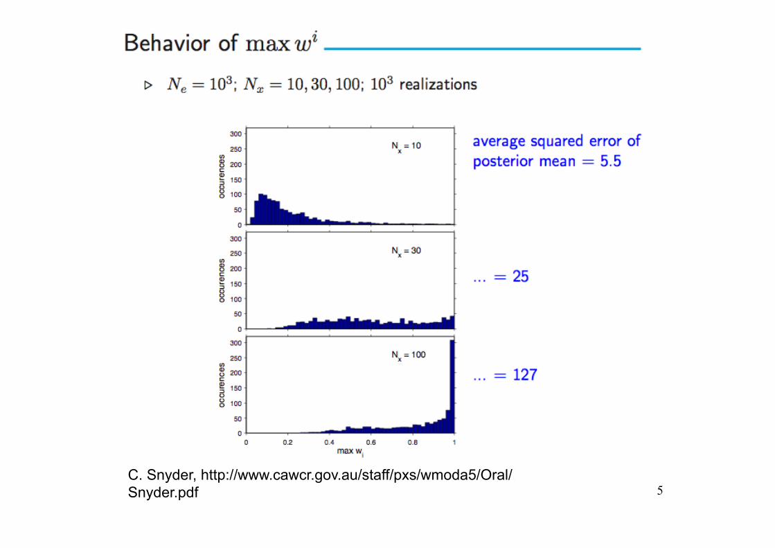
Curse of dimensionality

Standard one-dimensional gaussian random variable X

P[ ⎜X ⎜ < σ ] ≈ 0.84

In dimension n = 100, 0.84100 = 3.10-8

. 7

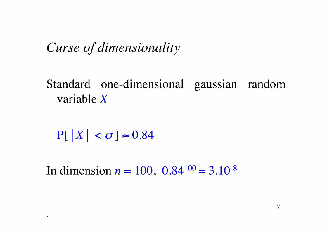
Bengtsson et al. (2008) and Snyder et al. (2008) evaluate that stability of filter requires the size of ensembles to increase exponentially with space dimension.

8

Alternative possibilities (review in van Leeuwen, 2017, Annales de la faculté des sciences de Toulouse Mathématiques, 26 (4), 1051-1085)

Resampling. Define new ensemble.

Simplest way. Draw new ensemble according to probability distribution defined by the updated weights. Give same weight to all particles. Particles are not modified, but particles with low weights are likely to be eliminated, while particles with large weights are likely to be drawn repeatedly. For multiple particles, add noise, either from the start, or in the form of ‘model noise’ in ensuing temporal integration.

Random character of the sampling introduces noise. Alternatives exist, such as residual sampling (Lui and Chen, 1998, van Leeuwen, 2003). Updated weights wl are multiplied by ensemble dimension L. Then p copies of each particle l are taken, where p is the integer part of Lwl. Remaining particles, if needed, are taken randomly from the resulting distribution.

However, resampling is not sufficient to avoid degeneracy of filters.

9

Idea :

Use a proposal density that is closer to the new observations than the density defined by the predicted particles (for instance the density defined by EnKF, after the latter has used the new observations).

10

van Leeuwen, 2017, Annales de la faculté des sciences de Toulouse Mathématiques, 26 (4), 1051-1085 11

van Leeuwen, 2017, ibid. 12

13

Several variants of proposal densities have been defined and studied : perform an EnKF up to observation time, and then use the obtained ensemble as proposal density, nudge the model integration between times n-1 and n towards the observations at time n, perform a 4D-Var on each particle, optimal proposal density, …

14

van Leeuwen, 2003, Mon. Wea. Rev., 131, 2071-2084

15

The Equivalent-Weights Particle Filter (Ades and van Leeuwen, QJRMS, 2013).

Make the proposal density depend on the whole ensemble at time n-1, and not only on xi

n-1, use density of the form q(xn | xn-1

1,L, yn), where 1,L denotes all ensemble indices, rather than of the more restrictive form q(xn | xi

n-1, yn). This gives many degrees of freedom which can be exploited for obtaining at time n an ensemble with almost equal weights.

16

Example Vorticity equation model with random error.

State-vector dimension ≈ 65,000 Decorrelation time: 25 timesteps One complete noisy model field

observed every 50 timesteps 24 particles

17

18

19

Bayesianity : experts say all these filters are bayesian (in the limit of infinite ensemble size)

Possible difficulties : numerical implementation, numerical cost

Particle filters are actively studied (van Leeuwen, Morzfeld, …)

20

-  Validation of assimilation algorithms

21

Unknown x to be determined. Belongs to state space S, with dimension n Data, belonging to data space D, with dimension m, available in the form

z = Γx + ζ

where Γ is a known (mxn)-matrix, rankΓ = n and ζ is ‘error’

Best Linear Unbiased Estimate (BLUE)

xa ≡ (Γ T S-1Γ)-1 Γ T S-1 [z - µ]

with µ = E(ζ) and S = E[(ζ- E(ζ) (ζ- E(ζ)T].

E(xa-x) = 0 E[(xa-x) (xa-x)T] ≡ Pa = (Γ T S-1Γ)-1

Determinacy condition : rankΓ = n. Data contain information, directly or indirectly, on every component of state vector x. Requires m ≥ n.

BLUE is invariant in any change of origin, or in any invertible linear transformation, in either data or state space. In particular, it is independent of the choice of a scalar product or norm in either of those spaces. BLUE minimizes the quadratic estimation error on any component of x. 22

If error ζ is gaussian, ζ ∼ N [µ, S], BLUE achieves bayesian estimation in the sense that

P(x | z) = N [xa, Pa]

Signification of xa and Pa is however different. In particular, in the gaussian gase, Pa is covariance matrix of conditional probability distribution of x for any data set z, while it is only, in the general BLUE case, the covariance of the estimation error xa-x, taken over all realizations of the error ζ.

The BLUE can be obtianed by minimization of the following scalar objective function, defined on state space X

ξ ∈ X → J(ξ) ≡ (1/2) [Γξ - (z-µ)]T S-1 [Γξ - (z-µ)]

Pa = [∂2J /∂ξ2]-1

J(ξ) is squared Mahalanobis norm of difference Γξ - (z-µ). That norm, which is associated with covariance matrix S. is defined on data space D.

23

Prasanta Chandra Mahalanobis (1893 -1972)"24

xa ≡ (Γ T S-1Γ)-1 Γ T S-1 [z - µ]

Determination of the BLUE requires (at least apparently) the a priori specification of the expectation and covariance matrix, i. e. the statistical moments of orders 1 and 2, of the error. The expectation is required for debiasing the data in the first place.

25

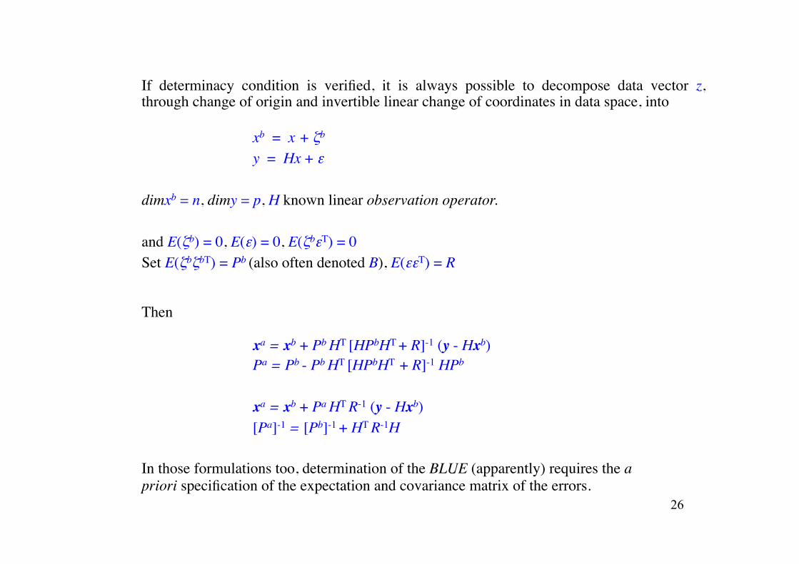
If determinacy condition is verified, it is always possible to decompose data vector z, through change of origin and invertible linear change of coordinates in data space, into

xb = x + ζb y = Hx + ε

dimxb = n, dimy = p, H known linear observation operator.

and E(ζb) = 0, E(ε) = 0, E(ζbεT) = 0 Set E(ζbζbT) = Pb (also often denoted B), E(εεT) = R

Then xa = xb + Pb

HT [HPbHT + R]-1 (y - Hxb)

Pa = Pb - Pb

HT [HPbHT

+ R]-1 HPb xa = xb + Pa

HT R-1 (y - Hxb)

[Pa]-1 = [Pb]-1 + HT

R-1H

In those formulations too, determination of the BLUE (apparently) requires the a priori specification of the expectation and covariance matrix of the errors.

26

Questions ���

  Is it possible to objectively evaluate the quality of an assimilation system ?

  Is it possible to objectively evaluate the first- and second-order statistical moments of the data errors, whose specification is required for determining the BLUE ?

  Is it possible to objectively determine whether an assimilation system is optimal ?

  More generally, how to make the best of an assimilation system ?

27

Objective validation

Objective validation is possible only by comparison with unbiased independent observations, i. e. observations that have not been used in the asssimilation, and that are affected with errors that are statistically independent of the errors affecting the data used in the assimilation.

Amplitude of forecast error, if estimated against observations that are really independent of observations used in assimilation, and everything else being the same, is an objective measure of quality of assimilation.

28

J(ξ) ≡ (1/2) [Γξ - (z-µ)]T S-1 [Γξ - (z-µ)]

z-µ

Γxa

Γ(S)

29

Minimizing J(ξ) amounts to

  debias z

  project orthogonally onto space Γ(S) according to Mahalanobis S-metric

  take inverse through Γ (inverse unambiguously defined through determinacy condition)

Computation of the BLUE is a generalized (Moore-Penrose) inverse. (Γ T S-1Γ)-1 Γ T S-1 is a left-inverse of Γ. Conversely, any left-inverse of Γ is of the form (Γ T Σ-1Γ)-1 Γ T Σ-1, with Σ a (non-uniquely defined) symmetric positive definite mxm matrix.

30

Decompose data space D into image space Γ(S) (index 1) and its S-orthogonal space ⊥Γ(S) (index 2)

Γ1 invertible

Set

Then xa = Γ1

-1 [z1 - µ1]

Pa = (Γ1 T S1

-1Γ1)-1

€

€

Γ =Γ10⎛

⎝ ⎜

⎞

⎠ ⎟

€

µ =µ1µ2

⎛

⎝ ⎜

⎞

⎠ ⎟

€

z =z1 = Γ1x + ζ1z2 = ζ 2

⎛

⎝ ⎜

⎞

⎠ ⎟

€

S =S1 00 S2

⎛

⎝ ⎜

⎞

⎠ ⎟

31

xa = Γ1 -1

[z1 - µ1]

The probability distribution of the error xa - x = Γ1

-1 [ζ1 - µ1]

depends on the probability distribution of ζ1.

On the other hand, the probability distribution of

δ = (z-µ) - Γxa =

depends only on the probability distribution of ζ2.

€

€

0ζ 2 −µ2

⎛

⎝ ⎜

⎞

⎠ ⎟

32

Contrary to what equations suggest, complete specification of expectation µ and covariance matrix S is not necessary for determining xa and Pa. It suffices to specify the subspace ⊥Γ(S) which is S-orthogonal to the image subspace Γ(S) in data space, and the respective components µ1 and S1 of µ and S along Γ(S) .

Practical implications ? Actually, not many. Data space D varies every day with observing system, and the above decomposition varies accordingly. It is only in the case of a stationary observing system (i.e., a system in which D, Γ, µ and S did not vary) that the above decomposition would be practically useful. Even if some components of the observing system are permanent (e.g., observation operators and/or variances of associated errors), one can think it will in general be preferable to introduce those permanent components as such in a general estimation algorithm, rather than modifying the algorithm as such.

33

Evaluation of first- and second-order moments of error statistics ?

Systematic search among all possible µ and S, i. e. performing assimilations for each possible couple (µ, S), and then evaluating results against independent observations ? Forget it.

Cross-validation (Wahba and others). For given instrument, search among possible values for error variance through validation against independent observations. Possible, may not have been sufficiently considered.

34

(Γ T S-1Γ)-1 Γ T S-1 is left-inverse of Γ for any S ⇒ Estimation schemes of the form

xa = (Γ T S-1Γ)-1 Γ T S-1 z (1)

will not spoil exact data.

In background-observation (xb, y) format, same property holds for schemes of the form

xa = xb + K (y - Hxb) (2)

where ‘gain matrix’ K is any nxp matrix (and holds only for those schemes). We will consider a scheme of form (1-2), built on a priori assumed (but not

necessarily correct) error statistics, and try and determine whether a possible misspecification of those statistics can be detected, and then corrected.

35

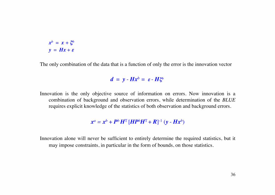
xb = x + ζb y = Hx + ε

The only combination of the data that is a function of only the error is the innovation vector

d = y - Hxb = ε - Hζb

Innovation is the only objective source of information on errors. Now innovation is a combination of background and observation errors, while determination of the BLUE requires explicit knowledge of the statistics of both observation and background errors.

xa = xb + Pb HT

[HPbHT + R]-1 (y - Hxb)

Innovation alone will never be sufficient to entirely determine the required statistics, but it may impose constraints, in particular in the form of bounds, on those statistics.

36

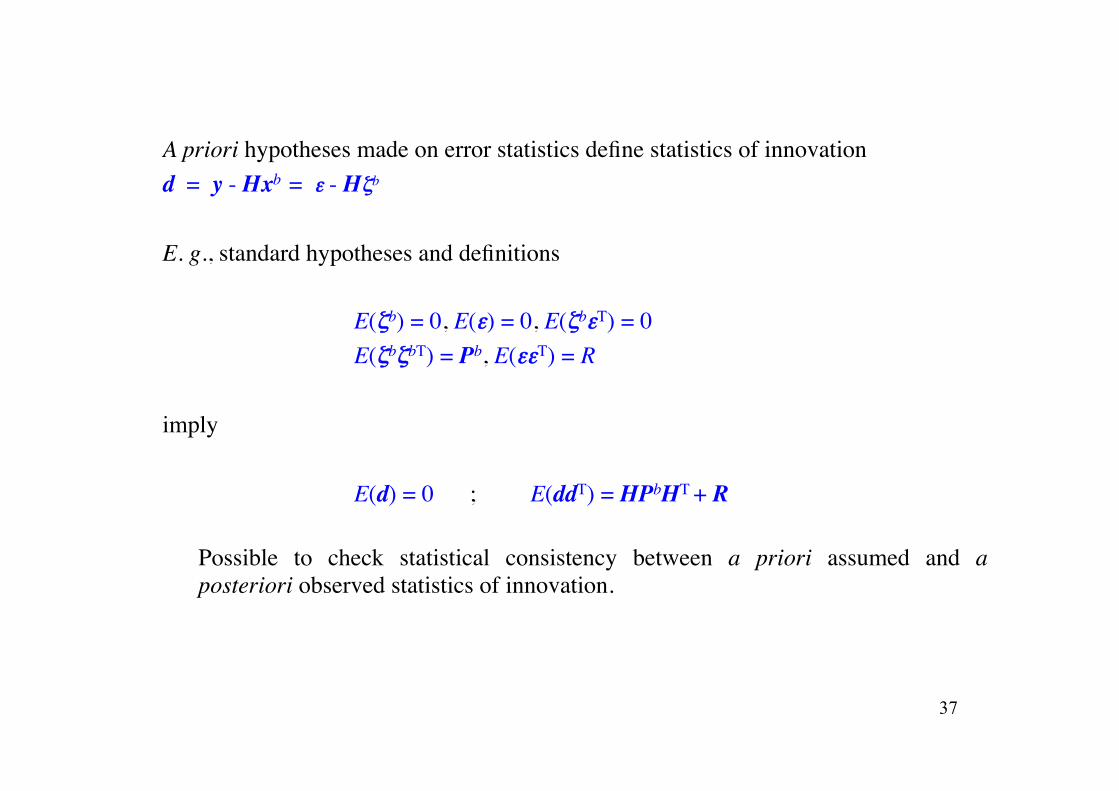
A priori hypotheses made on error statistics define statistics of innovation d = y - Hxb = ε - Hζb

E. g., standard hypotheses and definitions

E(ζb) = 0, E(ε) = 0, E(ζbεT) = 0 E(ζbζbT) = Pb, E(εεT) = R

imply

E(d) = 0 ; E(ddT) = HPbHT + R

Possible to check statistical consistency between a priori assumed and a posteriori observed statistics of innovation.

37

Data-minus-Analysis (DmA) difference δ = z - Γxa

For given gain matrix K, one-to-one correspondance d ⇔ δ It is exactly equivalent to compute statistics on either the innovation d or

on the DmA difference δ.

δ ≡x b − xa

y −Hxa⎛

⎝ ⎜ ⎜

⎞

⎠ ⎟ ⎟ =

−Kd(Ip − HK)d⎛

⎝ ⎜ ⎜

⎞

⎠ ⎟ ⎟

38

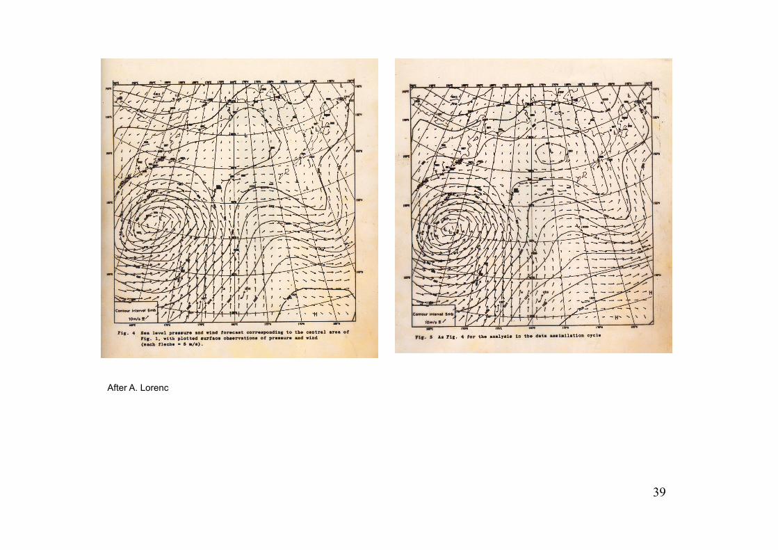
After A. Lorenc

39

For perfectly consistent system (i. e., system that uses the exact error statistics):

E(d) = 0 ( ⇔ E(δ) = 0)

Any systematic bias in either the innovation vector or the DmA difference is the signature of an inappropriately-taken-into-account bias in either the background or the observation (or both).

Primary diagnostic to perform on analysis system

40

In z-form, DmA difference reads

δ = (S - Γ PaΓT) S-1 z

= (S - Γ PaΓT) S-1 ζ

And, for a perfectly consistent system

E(δδT) = S - Γ PaΓT A perfectly consistent analysis statistically fits the data to within their own

accuracy.

If new data are added to (removed from) an optimal analysis system, DmA difference must increase (decrease).

41

Assume inconsistency has been found between a priori assumed and a posteriori observed statistics of innovation or DmA difference.

- What can be done ?

or, equivalently

- Which bounds does the knowledge of the statistics of innovation put on the error statistics whose knowledge is required by the BLUE ?

42

J(ξ) ≡ (1/2) [Γξ - (z-µ)]T S-1 [Γξ - (z-µ)]

z-µ

Γxa

Γ(S)

43

DmA difference, i. e. (z-µ) - Γxa, is in effect ‘rejected’ by the assimilation. Its expectation and covariance are irrelevant for the assimilation.

Consequence. Any assimilation scheme (i. e., a priori subtracted bias and gain matrix K) is compatible with any observed statistics of either DmA or innovation. Not only is not consistency between a priori assumed and a posteriori observed statistics of innovation (or DmA) sufficient for optimality of an assimilation scheme, it is not even necessary.

44

Example z1 = x + ζ1 z2 = x + ζ2

Errors ζ1 and ζ2 assumed to be centred (E(ζ1) = E(ζ2) = 0), to have same variance s and to be mutually uncorrelated.

Then

xa = (1/2) (z1 + z2) with expected quadratic estimation error

E[(xa-x)2] = s/2

Innovation is difference z1 - z2. With above hypotheses, one expects to observe

E(z1 - z2) = 0 ; E[(z1 - z2)2] = 2s

Assume one observes

E(z1 - z2) = b ; E[(z1 - z2)2] = b2 + 2γ

Inconsistency if b≠0 and/or γ≠s

45

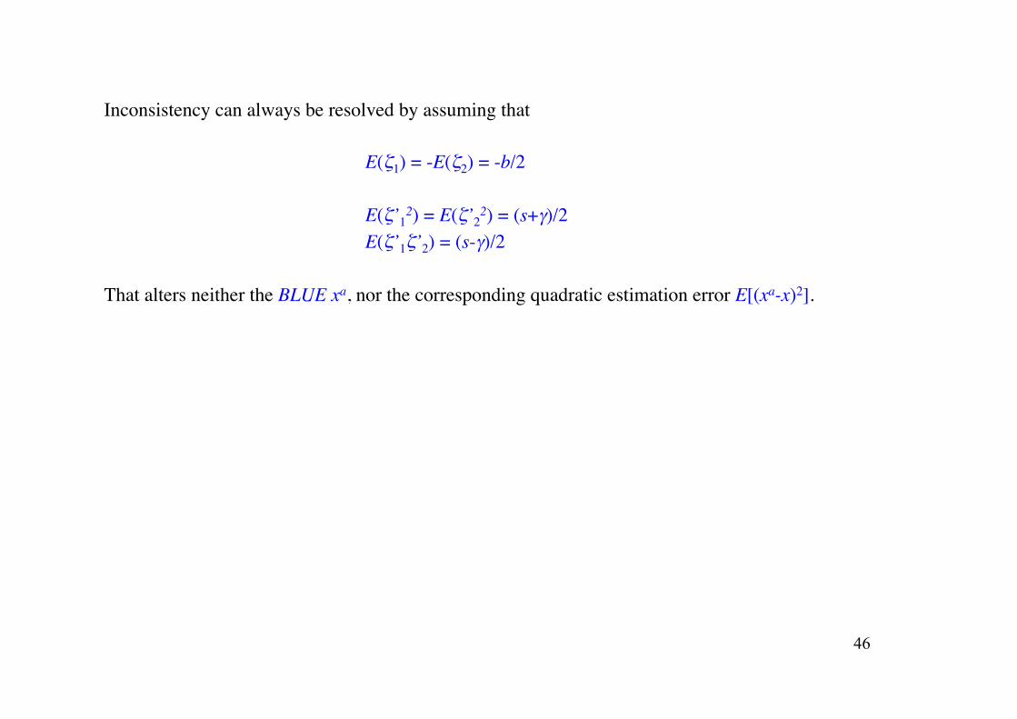
Inconsistency can always be resolved by assuming that

E(ζ1) = -E(ζ2) = -b/2

E(ζ’12) = E(ζ’2

2) = (s+γ)/2 E(ζ’1ζ’2) = (s-γ)/2

That alters neither the BLUE xa, nor the corresponding quadratic estimation error E[(xa-x)2].

46

Explanation. It is not necessary to know explicitly the complete expectation µ and covariance matrix S in order to perform the assimilation, and to determine the associated estimation error covariance matrix. A number of degrees of freedom are therefore useless for the assimilation, and can therefore be used, in infinitely many ways, to resolve any observed inconsistency between a priori and a posteriori observed statistics of the innovation d. The parameters determined by the statistics of d are equal in number, for both expectation and covariance, to those useless degrees of freedom. As a consequence, among the infinitely many possibilities for resolving the inconsistency, there is one in which neither the analysis nor its associated error covariance matrix is modified.

However, it may be that resolving the inconsistency in that way requires

conditions that are (independently) known to be very unlikely, if not simply impossible. For instance, in the above example, consistency when γ≠s requires the errors ζ1 and ζ2 to be mutually correlated, which may be known to be very unlikely.

47

Now, a resolution of the inconsistency that would change the orthogonal subspace ⊥Γ(S) would modify the analysis.

48

That result, which is purely mathematical, means that the specification of the error statistics required by the assimilation must always be entirely based, in the last resort, on external hypotheses, i. e. on hypotheses that cannot be objectively validated on the basis of the innovation alone. Given an inconsistency between a priori assumed and a posteriori observed innovation statistics, there is no mathematically fool-proof method for identifying the origin of the inconsistency.

Question. Does this result hold true in a general nonlinear case ? I don’t know. If anyone knows, tell me …

49

Problem. Identify hypotheses

  That will not be questioned (errors on observation performed a long distance apart by radiosondes made by different manufacturers are uncorrelated)

  That sound reasonable, but may be questioned (background errors are uncorrelated at scales of, say, 5000 km)

  That certainly look questionable (background and observation errors are mutually uncorrelated)

  That are undoubtedly questionable (model errors are negligible, or are uncorrelated in time)

Ideally, define a minimum set of hypotheses such that all remaining undetermined error

statistics can be objectively determined from observed statistics of innovation.

50

Hollingsworth and Lönnberg method

(From Bouttier and Courtier, ECMWF) 51

Use of innovations to estimate model errors (Q)

52

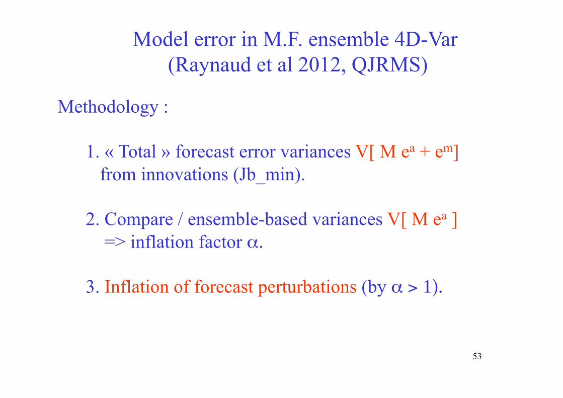
Model error in M.F. ensemble 4D-Var (Raynaud et al 2012, QJRMS)

Methodology :

1. « Total » forecast error variances V[ M ea + em] from innovations (Jb_min).

2. Compare / ensemble-based variances V[ M ea ] => inflation factor α.

3. Inflation of forecast perturbations (by α > 1).

53

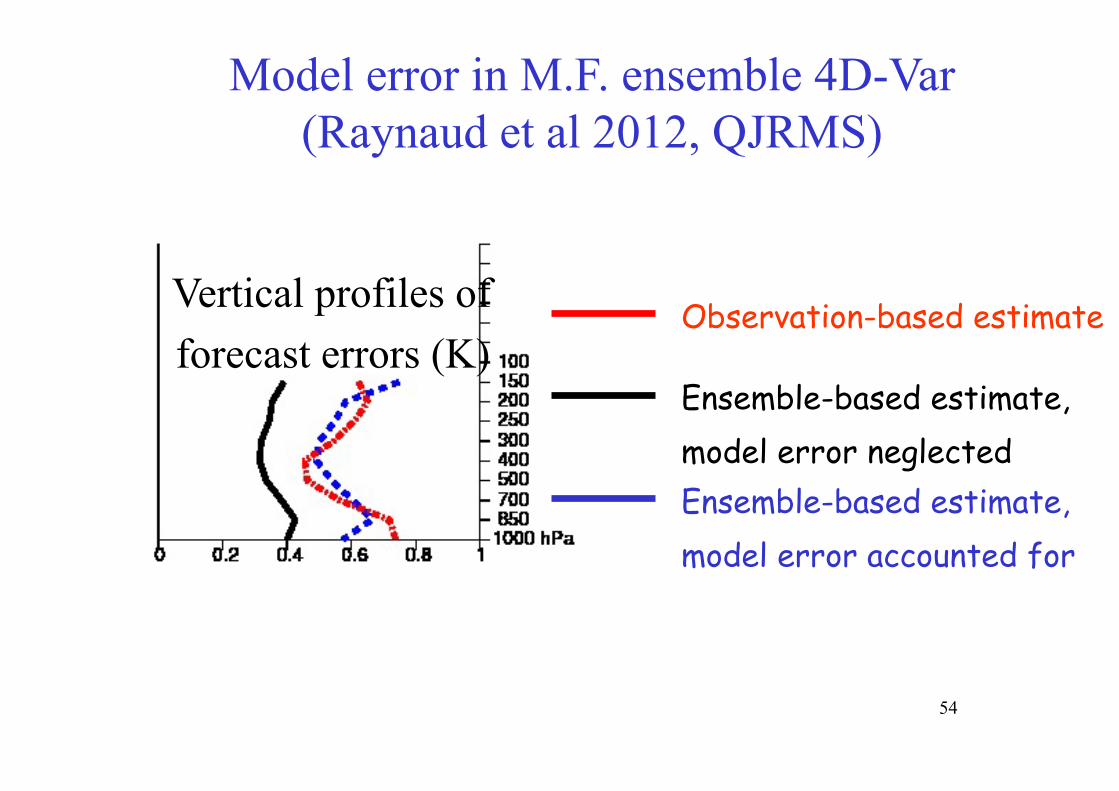
Model error in M.F. ensemble 4D-Var (Raynaud et al 2012, QJRMS)

Ensemble-based estimate, model error neglected Ensemble-based estimate, model error accounted for

Observation-based estimate Vertical profiles of forecast errors (K)

54

Model error in M.F. ensemble 4D-Var

  Inflation of forecast perturbations by 15% every 6h.

  Much more realistic initial spread (by a factor 2-3)

for ensemble prediction.

  A vertical and latitudinal dependence is needed

w.r.t. high level tropical winds.

  Neutral impact of new variances on the forecast quality.

L. Berre 55

Objective function

J(ξ) ≡ (1/2) [Γξ - z]T S-1 [Γξ - z]

Jmin ≡ J(xa) = (1/2) [Γxa - z]T S-1 [Γxa - z]

= (1/2) dT [E(ddT)]-1 d

⇒ E(Jmin) = p/2 (p = dimy = dimd)

If p is large, a few realizations are sufficient for determining E(Jmin) If observed E(Jmin) > p/2, amplitude of innovation is a priori underestimated, and overestimated if

E(Jmin) < p/2

Often called χ2 criterion.

Remark. If in addition errors are gaussian Var(Jmin) = p/2

56

57

Linearized Lorenz’96. 5 days. Histogram of Jmin E(Jmin) = p/2 (=200) ; σ(Jmin) = √(p/2) (≈14.14)

From course 7

Results for ECMWF (January 2003, n = 8.106)

- Operations (p = 1.4 106, has almost doubled since then)

2Jmin /p = 0.40 - 0.45

Innovation is significantly smaller than implied by Pb and R (a residual bias in d would make Jmin too large).

- Assimilation without satellite observations (p = 2 - 3 105)

2Jmin /p = 1. - 1.05

Similar results obtained at other NWP centres (C. Fischer, W. Sadiki with Aladin model, T. Payne at Meteorological Office, UK).

Probable explanation: error variance of satellite observations overestimated in order to compensate for ignored spatial correlation.

58

Informative content

Objective function J(ξ) = Σk Jk(ξ)

where Jk(ξ) ≡ (1/2) (Hkξ - yk)T Sk

-1 (Hkξ - yk)

with dimyk = mk

Accuracy of analysis Pa = (Γ T S-1Γ)-1

[Pa]-1 = Σk HkT Sk

-1 Hk

1 = (1/n) Σk tr(Pa HkT Sk

-1 Hk) = (1/n) Σk tr(Sk

–1/2 Hk Pa HkT Sk

–1/2)

59

Informative content (continuation 1)

(1/n) Σk tr(Sk–1/2 Hk Pa Hk

T Sk–1/2 ) = 1

I(yk) ≡ (1/n) tr(Sk–1/2 Hk Pa Hk

T Sk–1/2) is a measure of the relative contribution of subset of

data yk to overall accuracy of assimilation. Invariant in linear change of coordinates in data space ⇒ valid for any subset of data.

In particular

I(xb) = (1/n) tr[Pa (Pb)-1] = 1 - (1/n) tr(KH) I(y) = (1/n) tr(KH)

Rodgers, 2000, calls those quantities Degrees of Freedom for Signal, or for Noise, depending on whether considered subset belongs to ‘observations’ or ‘background’.

60

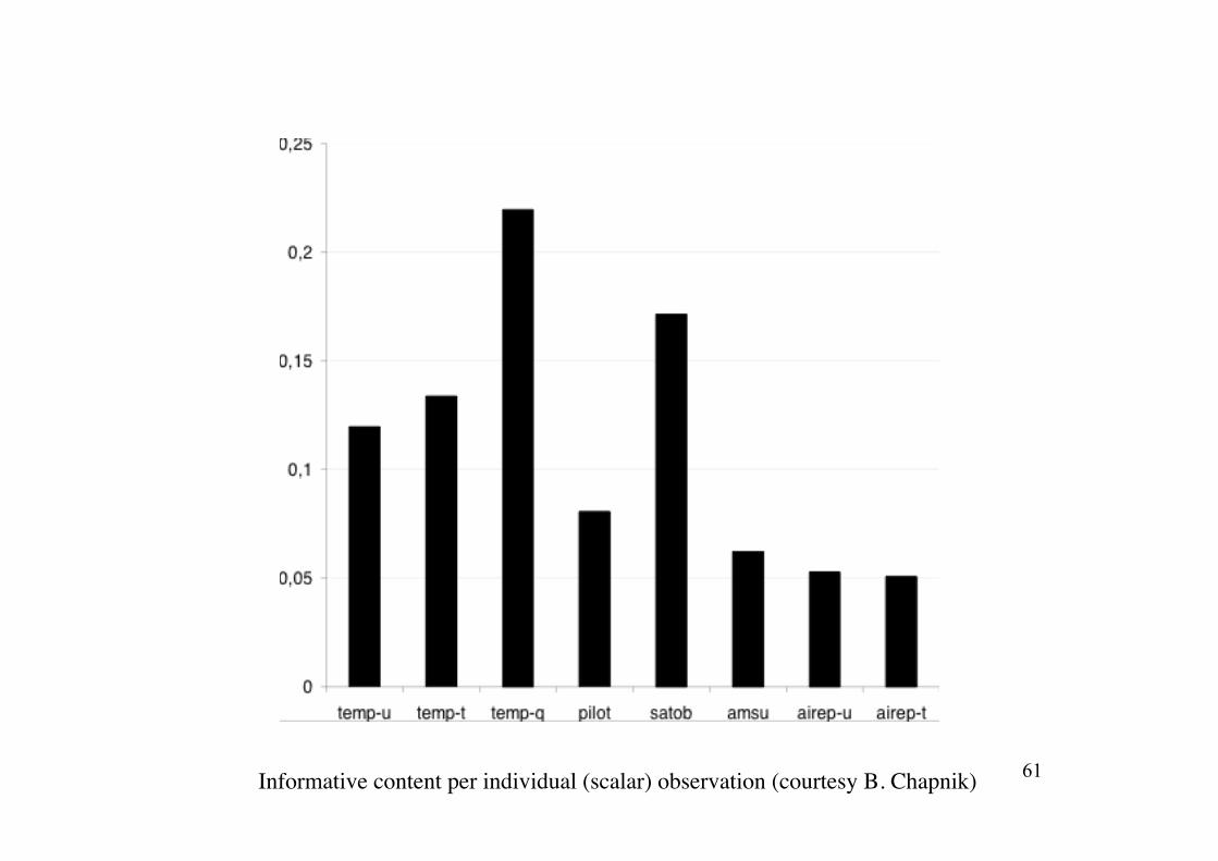
Informative content per individual (scalar) observation (courtesy B. Chapnik) 61

Objective function J(ξ) = Σk Jk(ξ)

where Jk(ξ) ≡ (1/2) (Hkξ - yk)T Sk

-1 (Hkξ - yk) with dimyk = mk

For a perfectly consistent system

E[Jk(xa)] = (1/2) [mk - tr(Sk–1/2 Hk Pa Hk

T Sk–1/2)]

(in particular, E(Jmin) = p/2)

For same vector dimension mk, more informative data subsets lead at the minimum to smaller terms in the objective function.

62

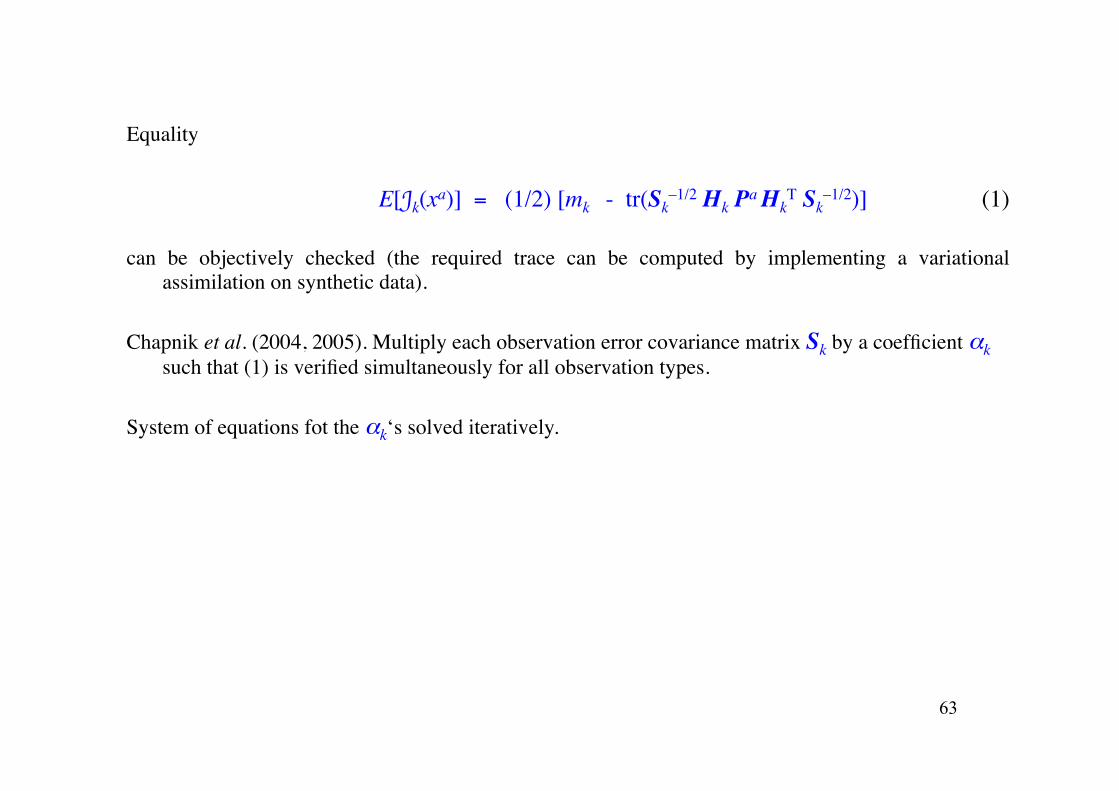
Equality

E[Jk(xa)] = (1/2) [mk - tr(Sk–1/2 Hk Pa Hk

T Sk–1/2)] (1)

can be objectively checked (the required trace can be computed by implementing a variational assimilation on synthetic data).

Chapnik et al. (2004, 2005). Multiply each observation error covariance matrix Sk by a coefficient αk such that (1) is verified simultaneously for all observation types.

System of equations fot the αk‘s solved iteratively.

63

Chapnik et al., 2006, QJRMS, 132, 543-565 64

Informative content (continuation 2)

I(yk) ≡ (1/n) tr(Sk–1/2 Hk Pa Hk

T Sk–1/2)

Two subsets of data z1 and z2

If errors affecting z1 and z2 are uncorrelated, then I(z1 ∪ z2) = I(z1) + I(z2)

If errors are correlated I(z1 ∪ z2) ≠ I(z1) + I(z2)

If I(z1 ∪ z2) < I(z1) + I(z2), subsets z1 and z2 can be said to be positively correlated, and negatively correlated if I(z1 ∪ z2) > I(z1) + I(z2)

65

Informative content (continuation 3)

Example 1 z1 = x + ζ1

z2 = x + ζ2

Errors ζ1 and ζ2 assumed to be centred, to have same variance and correlation coefficient c.

I(z1) = I(z2) = (1/2) (1 + c)

Example 2

State vector x evolving in time according to

x2 = α x1 Observations are performed at times 1 and 2. Observation errors are assumed centred, uncorrelated and with same

variance. Information contents are then in ratio (1/α , α). For an unstable system (α >1), later observation contains more information (and the opposite for a stable system).

66

Informative content (continuation 4)

Subset u1 of analyzed fields, dimu1 = n1. Define relative contribution of subset yk of data to accuracy of u1?

u2 : component of x orthogonal to u1 with respect to Mahalanobis norm associated with Pa

(analysis errors on u1 and u2 are uncorrelated).

x = (u1T, u2

T)T. In basis (u1, u2)

Pa =Pa

1 00 Pa

2

⎛

⎝ ⎜ ⎜

⎞

⎠ ⎟ ⎟

67

Informative content (continuation 5)

Observation operator Hk decomposes into

Hk = (Hk1 Hk2)

and expression of estimation error covariance matrix into

[Pa1]-1 = Σk Hk1

T Sk-1 Hk1

[Pa2]-1 = Σk Hk2

T Sk-1 Hk2

Same development as before shows that the quantity

(1/n1) tr(Sk–1/2 Hk1 Pa

1 Hk1

T Sk–1/2)

is a measure of the relative contribution of subset yk of data to analysis of subset u1 of state vector.

But can it be computed in practice for large dimension systems (requires the explicit decomposition x = (u1

T, u2T)T) ?

68

Other possible diagnostics (Desroziers et al., 2006)

If background and observation errors are assumed to be unbiased and mutually uncorrelated, then

E(ddT) = HPbHT + R

If HPbHT invertible, this is equivalent to

E[H(xa-xb)(y-Hxb)T] = E[H(xa-xb)dT] = HPbHT

And, if R invertible, to

E[(y-Hxa)(y-Hxb)T] = E[(y-Hxa)dT] = R

69

Optimality

Equation

xa = xb - E(ζbdT) [E(ddT)]-1 (y - Hxb)

means that estimation error x - xa is uncorrelated with innovation y - Hxb (if it was not, it would be possible to improve on xa by statistical linear estimation).

Independent unbiased observation

v = Cx + γ

Fit to analysis v - Cxa = C(x - xa) + γ

E[(v - Cxa) dT] = CE[(x - xa) dT] + E(γ dT)

First term is 0 if analysis is optimal, second is 0 if observation v is independent from previous data.

Daley (1992)

70

Conclusions

  Absolute evaluation of analysis schemes, and comparison between different schemes

Can be evaluated only against independent unbiased data (independence and unbiasedness cannot be objectively checked). Fundamental, but not much to say.

  Determination of required statistics

Impossible to achieve in a purely objective way. Will always require physical knowledge, educated guess, interaction with instrumentalists and modelers, and the like.

Inconsistencies in specification of statistics can be objectively diagnosed, and can help in improving assimilation.

For given error statistics, possible to quantify relative contribution of each subset of data to analysis of each subset of state vector.

(and also Generalized Cross-Validation, Adaptive Filtering)

  Optimality of analysis schemes

Optimality in the sense of least error variance can be objectively checked against independent unbiased data.

71

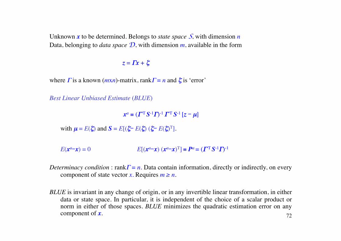
Unknown x to be determined. Belongs to state space S, with dimension n Data, belonging to data space D, with dimension m, available in the form

z = Γx + ζ

where Γ is a known (mxn)-matrix, rankΓ = n and ζ is ‘error’

Best Linear Unbiased Estimate (BLUE)

xa ≡ (Γ T S-1Γ)-1 Γ T S-1 [z - µ]

with µ = E(ζ) and S = E[(ζ- E(ζ) (ζ- E(ζ)T].

E(xa-x) = 0 E[(xa-x) (xa-x)T] ≡ Pa = (Γ T S-1Γ)-1

Determinacy condition : rankΓ = n. Data contain information, directly or indirectly, on every component of state vector x. Requires m ≥ n.

BLUE is invariant in any change of origin, or in any invertible linear transformation, in either data or state space. In particular, it is independent of the choice of a scalar product or norm in either of those spaces. BLUE minimizes the quadratic estimation error on any component of x. 72

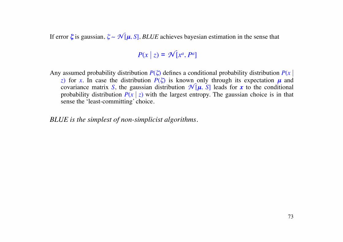
If error ζ is gaussian, ζ ∼ N [µ, S], BLUE achieves bayesian estimation in the sense that

P(x | z) = N [xa, Pa]

Any assumed probability distribution P(ζ) defines a conditional probability distribution P(x | z) for x. In case the distribution P(ζ) is known only through its expectation µ and covariance matrix S, the gaussian distribution N [µ, S] leads for x to the conditional probability distribution P(x | z) with the largest entropy. The gaussian choice is in that sense the ‘least-committing’ choice.

BLUE is the simplest of non-simplicist algorithms.

73

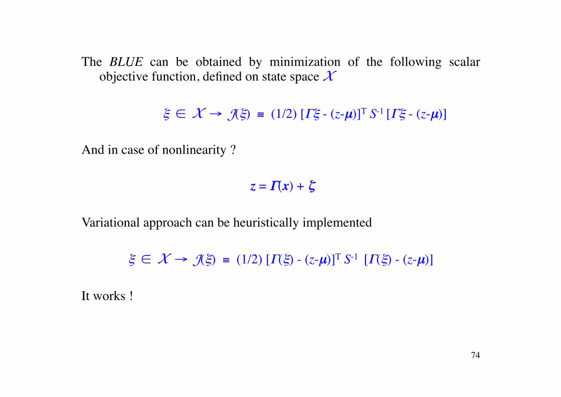
The BLUE can be obtained by minimization of the following scalar objective function, defined on state space X

ξ ∈ X → J(ξ) ≡ (1/2) [Γξ - (z-µ)]T S-1 [Γξ - (z-µ)]

And in case of nonlinearity ?

z = Γ(x) + ζ

Variational approach can be heuristically implemented

ξ ∈ X → J(ξ) ≡ (1/2) [Γ(ξ) - (z-µ)]T S-1 [Γ(ξ) - (z-µ)]

It works !

74

If data are of the form (after possibly an appropriate transformation) xb = x + ζb y = H(x) + ε

Transformation

xb = x + ζb y - H(xb) = H(x) - H(xb) + ε ≈ H’(x - xb) + ε

where H’ is jacobian of H, makes the estimation problem linear in the deviation x – xb (tangent linear approximation)

All algorithms that have been presented in the course, with the exception of particle filters, are empirical heuristic extensions of the BLUE approach to approximate nonlinear and non-gaussian situations.

75

76

Assimilation, which originated from the need of defining initial conditions for numerical weather forecasts, has gradually extended to many diverse applications

•  Oceanography •  Palaoclimatology •  Atmospheric chemistry (both troposphere and stratosphere) •  Oceanic biogeochemistry •  Ground hydrology •  Terrestrial biosphere and vegetation cover •  Glaciology •  Magnetism (both planetary and stellar) •  Plate tectonics •  Planetary atmospheres (Mars, …) •  Reassimilation of past observations (mostly for climatological purposes, ECMWF, NCEP/NCAR) •  Identification of source of tracers •  Parameter identification •  A priori evaluation of anticipated new instruments •  Definition of observing systems (Observing Systems Simulation Experiments) •  Validation of models •  Sensitivity studies (adjoints) •  Mathematical studies, independently of direct real life applications •  …

It has now become a major tool of numerical environmental science, and a subject of mathematical study in its own right.

A few of the (many) remaining problems :

  Observability (what to observe in order to know what we want to know ? Data are noisy, system is chaotic !)

  More accurate identification and quantification of errors affecting data particularly the assimilating model (will always require independent hypotheses)

  Assimilation of images

  …

77

La Fin du Cours …

79