Embed Size (px)
Citation preview
© 2010-2018 F. Dellsperger
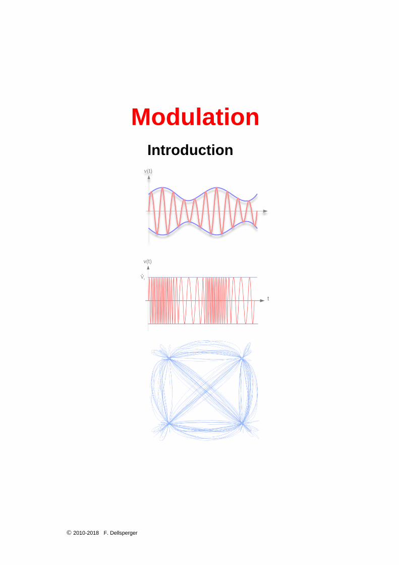
Introduction
Modulation
© 2010-2018 F. Dellsperger
Content
1. Introduction to Modulation ..................................................................................................... 1
1.1 Access methods, bundling of signals ...................................................................................... 3
1.2 Useful Signal-Theory and Mathematical Methods ................................................................... 6
1.2.1 Classification of signals ....................................................................................................... 6
1.2.1.1 Deterministic signals .................................................................................................... 6
1.2.1.2 Random signals ........................................................................................................... 6
1.2.1.3 Causal signals ............................................................................................................. 7
1.2.1.4 Energy signals ............................................................................................................. 7
1.2.1.5 Power signals .............................................................................................................. 7
1.2.1.6 Analytic signal and Hilbert transformation ................................................................... 7
1.2.1.7 Continuous signals ...................................................................................................... 9
1.2.1.8 Discrete signals and sampling ..................................................................................... 9
1.2.2 Mathematical description and graphical representation of signals .................................... 11
1.2.2.1 Sine/Cosine signal ..................................................................................................... 11
1.2.2.2 Discrete cosine signal ................................................................................................ 14
1.2.2.3 Rectangular Pulse ..................................................................................................... 14
1.2.2.4 Dirac Impulse (Unit Impulse) ..................................................................................... 14
1.2.2.5 Sinc function (cardinal sine function) ......................................................................... 15
1.2.3 Fourier Series and Fourier Transformation ....................................................................... 16
1.2.3.1 Fourier Series and Fourier Transformation of continuous signals ............................ 16
1.2.3.2 Discrete Fourier Transformation DFT ........................................................................ 19
1.2.3.3 Examples: .................................................................................................................. 20
1.2.4 Convolution ........................................................................................................................ 26
1.2.4.1 Convolution of continuous signals ............................................................................. 26
1.2.4.2 Convolution of discrete signals .................................................................................. 30
1.2.5 Correlation ......................................................................................................................... 30
1.2.6 Energy and power spectrum density ................................................................................. 32
1.3 References ............................................................................................................................ 34
© 2010-2018 F. Dellsperger
Fig. 1-1: Reasons for modulation .................................................................................................. 1 Fig. 1-2: Modulation of pulse carrier .............................................................................................. 3 Fig. 1-3: Modulation of sinusoidal carrier ...................................................................................... 3 Fig. 1-4: Frequency allocation in FDMA systems ......................................................................... 4 Fig. 1-5: Time allocation in TDMA systems ................................................................................... 4 Fig. 1-6: Code allocation in CDMA systems.................................................................................. 5 Fig. 1-7: Modulated carriers in OFDM system .............................................................................. 6 Fig. 1-8: Phase shift of a Hilbert-Transformer ............................................................................... 7 Fig. 1-9: a) Real signal, b) Analytic signal ................................................................................... 8 Fig. 1-10: Continuous or analog signal ......................................................................................... 9 Fig. 1-11: Continuous and discrete signals ................................................................................... 9 Fig. 1-12: Analog signal and sampling function .......................................................................... 10 Fig. 1-13: Sampled analog signal ................................................................................................ 10 Fig. 1-14: Sampled analog signal, convolution in frequency domain .......................................... 10 Fig. 1-15: Aliasing, spectrum overlapping ................................................................................... 11 Fig. 1-16: Cosine signal in time domain, 0 .......................................................................... 12 Fig. 1-17: Cosine signal in frequency domain, magnitude spectrum of a cosine signal ............. 13 Fig. 1-18: Complex sinusoidal signal in phase diagram, phasor of complex sinusoidal signal .. 13 Fig. 1-19: Rectangular pulse ....................................................................................................... 14 Fig. 1-20: Dirac impulse .............................................................................................................. 14 Fig. 1-21: Sample at t0 ................................................................................................................. 15 Fig. 1-22: Sampling function........................................................................................................ 15 Fig. 1-23: Sinc function ................................................................................................................ 16 Fig. 1-24: Amplitude and Phase Spectrum of a discrete signal .................................................. 19 Fig. 1-25: Unipolar square wave, time domain and spectrum..................................................... 20 Fig. 1-26: Approximation of square wave using Fourier series ................................................... 21 Fig. 1-27: Bipolar square wave, time domain and spectrum ....................................................... 21 Fig. 1-28: Pulse train, time domain and spectrum ...................................................................... 22 Fig. 1-29: Pulse train, time domain and spectrum ...................................................................... 22 Fig. 1-30: Sampling function, time domain and spectrum ........................................................... 23 Fig. 1-31: Cosine signal, time domain and spectrum .................................................................. 23 Fig. 1-32: Sine signal, time domain and spectrum ...................................................................... 24 Fig. 1-33: Rectangular pulse, time domain and spectrum .......................................................... 24 Fig. 1-34: sinc-pulse, time domain and spectrum ....................................................................... 25 Fig. 1-35: Triangle pulse, time domain and spectrum ................................................................. 26 Fig. 1-36: Convolution in time domain of an arbitrary signal with a Dirac pulse ......................... 27 Fig. 1-37: Arbitrary signal and cosine signal:
a) Multiplication in time domain, b) convolution in frequency domain ................. 28 Fig. 1-38: Sampling of an arbitrary signal:
a) Multiplication in time domain, b) convolution in frequency domain ................. 29 Fig. 1-39: Autocorrelation function of a PN-Code with length 7 .................................................. 32 Fig. 1-40: Power spectrum density of a PN-Code with length 7 ................................................. 32
© 2010-2018 F. Dellsperger 1
1. Introduction to Modulation
In modern communication systems, the signal generated by the information source can normally not be transmitted directly. In the majority of cases, an adjustment to the physical channel, i.e. a coax cable, a wireless channel or an optical fiber, is necessary. For the purpose of the economical utilization of the channel, the bundling of different signals is common. For transmission in wireless communication systems, the use of sinusoidal carriers is common, with the information influencing their amplitude, frequency, phase or combinations of these characteristics. The term modulation means the changing of one or more signal parameters (amplitude, frequency or phase) of a carrier as a function of the information. Due to this, the information is “imprinted” onto the carrier signal.
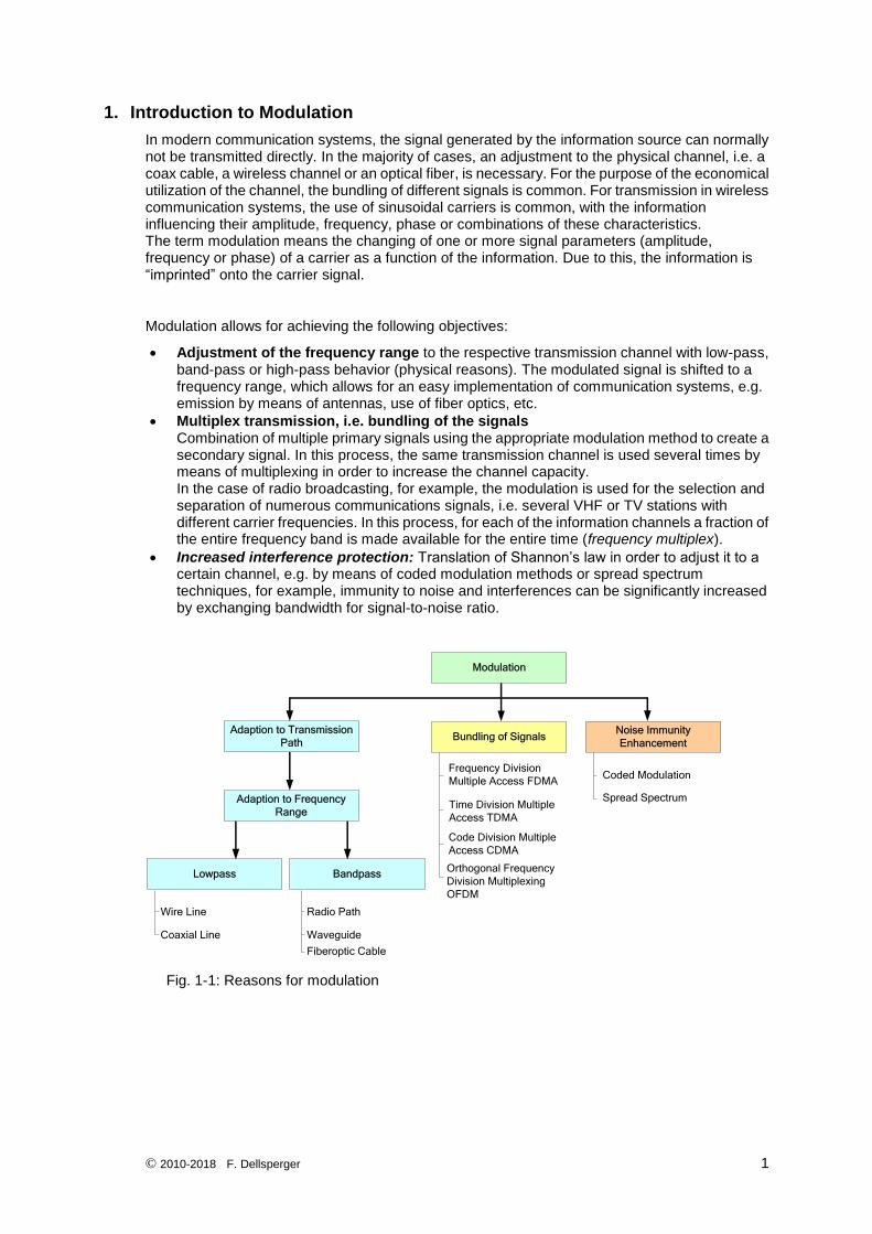
Modulation allows for achieving the following objectives:
Adjustment of the frequency range to the respective transmission channel with low-pass, band-pass or high-pass behavior (physical reasons). The modulated signal is shifted to a frequency range, which allows for an easy implementation of communication systems, e.g. emission by means of antennas, use of fiber optics, etc.
Multiplex transmission, i.e. bundling of the signals Combination of multiple primary signals using the appropriate modulation method to create a secondary signal. In this process, the same transmission channel is used several times by means of multiplexing in order to increase the channel capacity. In the case of radio broadcasting, for example, the modulation is used for the selection and separation of numerous communications signals, i.e. several VHF or TV stations with different carrier frequencies. In this process, for each of the information channels a fraction of the entire frequency band is made available for the entire time (frequency multiplex).
Increased interference protection: Translation of Shannon’s law in order to adjust it to a certain channel, e.g. by means of coded modulation methods or spread spectrum techniques, for example, immunity to noise and interferences can be significantly increased by exchanging bandwidth for signal-to-noise ratio.
Modulation
Adaption to Transmission
PathBundling of Signals
Noise Immunity
Enhancement
Adaption to Frequency
Range
Lowpass Bandpass
Wire Line
Coaxial Line
Radio Path
Waveguide
Fiberoptic Cable
Frequency Division
Multiple Access FDMA
Time Division Multiple
Access TDMA
Code Division Multiple
Access CDMA
Coded Modulation
Spread Spectrum
Orthogonal Frequency
Division Multiplexing
OFDM
Fig. 1-1: Reasons for modulation
© 2010-2018 F. Dellsperger 2
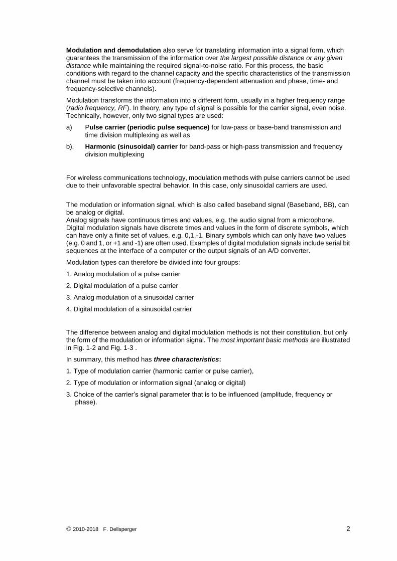
Modulation and demodulation also serve for translating information into a signal form, which guarantees the transmission of the information over the largest possible distance or any given distance while maintaining the required signal-to-noise ratio. For this process, the basic conditions with regard to the channel capacity and the specific characteristics of the transmission channel must be taken into account (frequency-dependent attenuation and phase, time- and frequency-selective channels).
Modulation transforms the information into a different form, usually in a higher frequency range (radio frequency, RF). In theory, any type of signal is possible for the carrier signal, even noise. Technically, however, only two signal types are used:
a) Pulse carrier (periodic pulse sequence) for low-pass or base-band transmission and time division multiplexing as well as
b). Harmonic (sinusoidal) carrier for band-pass or high-pass transmission and frequency division multiplexing
For wireless communications technology, modulation methods with pulse carriers cannot be used due to their unfavorable spectral behavior. In this case, only sinusoidal carriers are used.
The modulation or information signal, which is also called baseband signal (Baseband, BB), can be analog or digital. Analog signals have continuous times and values, e.g. the audio signal from a microphone. Digital modulation signals have discrete times and values in the form of discrete symbols, which can have only a finite set of values, e.g. 0,1,-1. Binary symbols which can only have two values (e.g. 0 and 1, or +1 and -1) are often used. Examples of digital modulation signals include serial bit sequences at the interface of a computer or the output signals of an A/D converter.
Modulation types can therefore be divided into four groups:
1. Analog modulation of a pulse carrier
2. Digital modulation of a pulse carrier
3. Analog modulation of a sinusoidal carrier
4. Digital modulation of a sinusoidal carrier
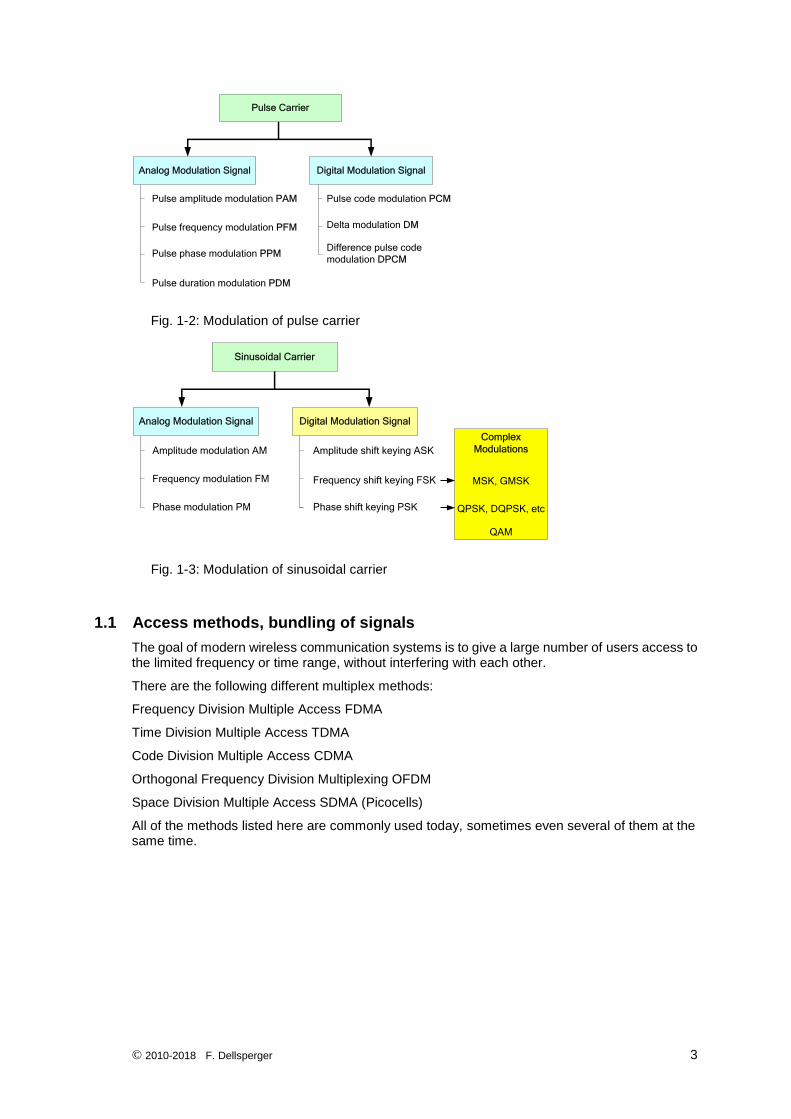
The difference between analog and digital modulation methods is not their constitution, but only the form of the modulation or information signal. The most important basic methods are illustrated in Fig. 1-2 and Fig. 1-3 .
In summary, this method has three characteristics:
1. Type of modulation carrier (harmonic carrier or pulse carrier),
2. Type of modulation or information signal (analog or digital)
3. Choice of the carrier’s signal parameter that is to be influenced (amplitude, frequency or phase).
© 2010-2018 F. Dellsperger 3
Pulse Carrier
Analog Modulation Signal Digital Modulation Signal
Pulse frequency modulation PFM
Pulse phase modulation PPM
Delta modulation DM
Pulse amplitude modulation PAM Pulse code modulation PCM
Difference pulse code
modulation DPCM
Pulse duration modulation PDM
Fig. 1-2: Modulation of pulse carrier
Sinusoidal Carrier
Analog Modulation Signal Digital Modulation Signal
Frequency modulation FM
Phase modulation PM
Frequency shift keying FSK
Phase shift keying PSK
Amplitude modulation AM Amplitude shift keying ASK
Complex
Modulations
MSK, GMSK
QPSK, DQPSK, etc
QAM
Fig. 1-3: Modulation of sinusoidal carrier
1.1 Access methods, bundling of signals
The goal of modern wireless communication systems is to give a large number of users access to the limited frequency or time range, without interfering with each other.
There are the following different multiplex methods:
Frequency Division Multiple Access FDMA
Time Division Multiple Access TDMA
Code Division Multiple Access CDMA
Orthogonal Frequency Division Multiplexing OFDM
Space Division Multiple Access SDMA (Picocells)
All of the methods listed here are commonly used today, sometimes even several of them at the same time.
© 2010-2018 F. Dellsperger 4
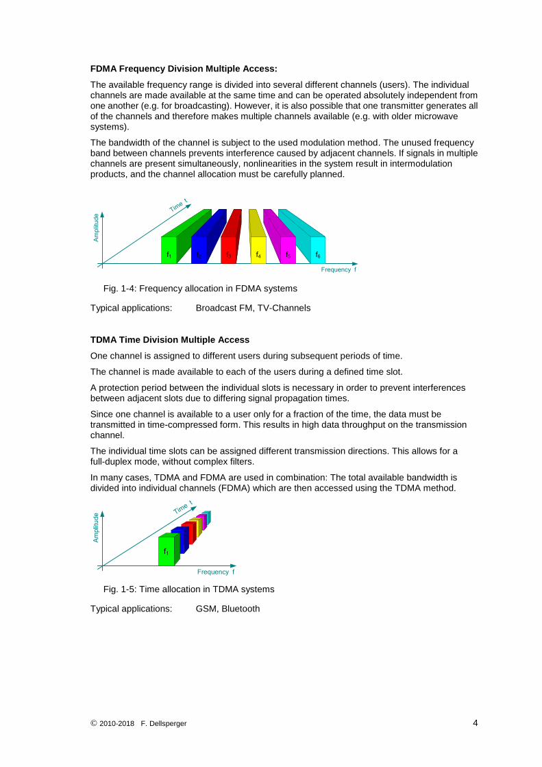
FDMA Frequency Division Multiple Access:
The available frequency range is divided into several different channels (users). The individual channels are made available at the same time and can be operated absolutely independent from one another (e.g. for broadcasting). However, it is also possible that one transmitter generates all of the channels and therefore makes multiple channels available (e.g. with older microwave systems).
The bandwidth of the channel is subject to the used modulation method. The unused frequency band between channels prevents interference caused by adjacent channels. If signals in multiple channels are present simultaneously, nonlinearities in the system result in intermodulation products, and the channel allocation must be carefully planned.
f6f1 f2 f3 f4 f5
Frequency f
Time t
Am
plit
ud
e
f6f1 f2 f3 f4 f5
Fig. 1-4: Frequency allocation in FDMA systems
Typical applications: Broadcast FM, TV-Channels
TDMA Time Division Multiple Access
One channel is assigned to different users during subsequent periods of time.
The channel is made available to each of the users during a defined time slot.
A protection period between the individual slots is necessary in order to prevent interferences between adjacent slots due to differing signal propagation times.
Since one channel is available to a user only for a fraction of the time, the data must be transmitted in time-compressed form. This results in high data throughput on the transmission channel.
The individual time slots can be assigned different transmission directions. This allows for a full-duplex mode, without complex filters.
In many cases, TDMA and FDMA are used in combination: The total available bandwidth is divided into individual channels (FDMA) which are then accessed using the TDMA method.
Frequency f
Time t
Am
plit
ud
e
f1
Fig. 1-5: Time allocation in TDMA systems
Typical applications: GSM, Bluetooth
© 2010-2018 F. Dellsperger 5
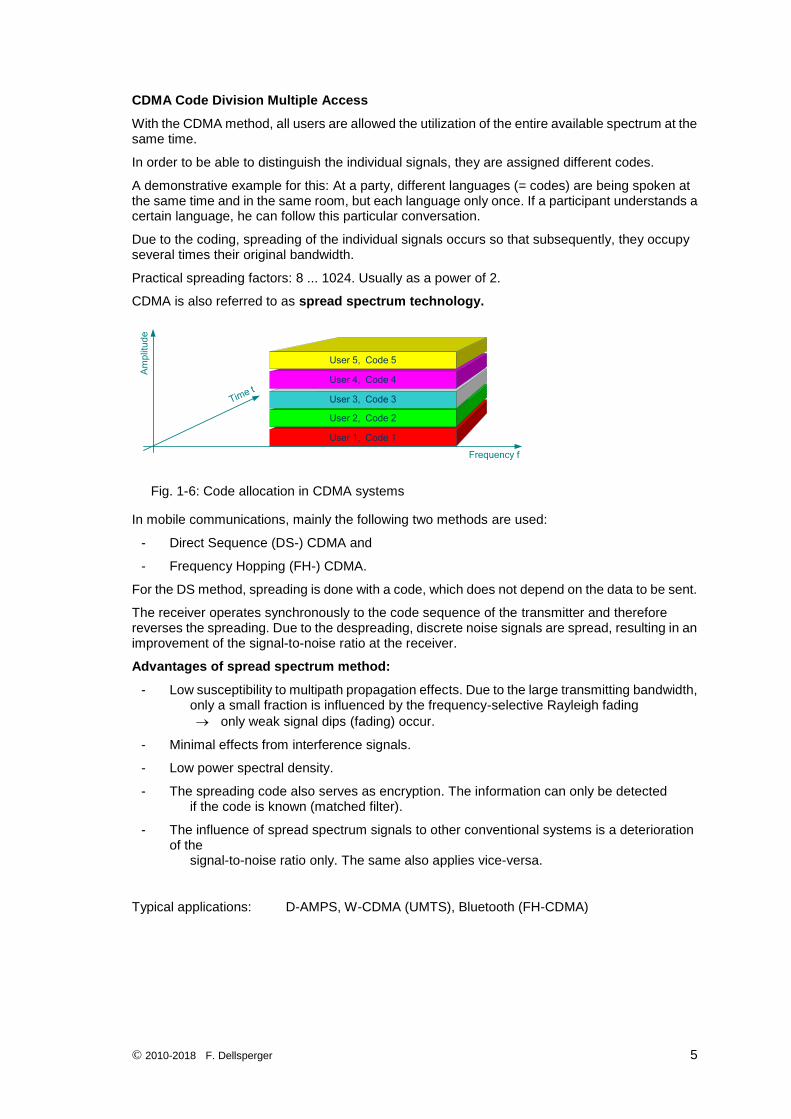
CDMA Code Division Multiple Access
With the CDMA method, all users are allowed the utilization of the entire available spectrum at the same time.
In order to be able to distinguish the individual signals, they are assigned different codes.
A demonstrative example for this: At a party, different languages (= codes) are being spoken at the same time and in the same room, but each language only once. If a participant understands a certain language, he can follow this particular conversation.
Due to the coding, spreading of the individual signals occurs so that subsequently, they occupy several times their original bandwidth.
Practical spreading factors: 8 ... 1024. Usually as a power of 2.
CDMA is also referred to as spread spectrum technology.
User 1, Code 1
User 2, Code 2
User 3, Code 3
User 4, Code 4
User 5, Code 5
Time t
Frequency f
Am
plit
ud
e
Fig. 1-6: Code allocation in CDMA systems
In mobile communications, mainly the following two methods are used:
- Direct Sequence (DS-) CDMA and
- Frequency Hopping (FH-) CDMA.
For the DS method, spreading is done with a code, which does not depend on the data to be sent.
The receiver operates synchronously to the code sequence of the transmitter and therefore reverses the spreading. Due to the despreading, discrete noise signals are spread, resulting in an improvement of the signal-to-noise ratio at the receiver.
Advantages of spread spectrum method:
- Low susceptibility to multipath propagation effects. Due to the large transmitting bandwidth, only a small fraction is influenced by the frequency-selective Rayleigh fading
only weak signal dips (fading) occur.
- Minimal effects from interference signals.
- Low power spectral density.
- The spreading code also serves as encryption. The information can only be detected if the code is known (matched filter).
- The influence of spread spectrum signals to other conventional systems is a deterioration of the signal-to-noise ratio only. The same also applies vice-versa.
Typical applications: D-AMPS, W-CDMA (UMTS), Bluetooth (FH-CDMA)
© 2010-2018 F. Dellsperger 6
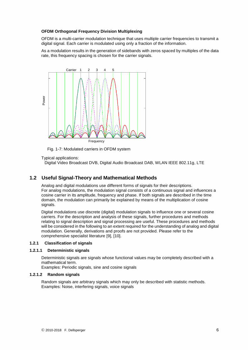
OFDM Orthogonal Frequency Division Multiplexing
OFDM is a multi-carrier modulation technique that uses multiple carrier frequencies to transmit a digital signal. Each carrier is modulated using only a fraction of the information.
As a modulation results in the generation of sidebands with zeros spaced by multiples of the data rate, this frequency spacing is chosen for the carrier signals.
Frequency
Po
we
r
Carrier 1 2 3 4 5
Fig. 1-7: Modulated carriers in OFDM system
Typical applications: Digital Video Broadcast DVB, Digital Audio Broadcast DAB, WLAN IEEE 802.11g, LTE
1.2 Useful Signal-Theory and Mathematical Methods
Analog and digital modulations use different forms of signals for their descriptions. For analog modulations, the modulation signal consists of a continuous signal and influences a cosine carrier in its amplitude, frequency and phase. If both signals are described in the time domain, the modulation can primarily be explained by means of the multiplication of cosine signals.
Digital modulations use discrete (digital) modulation signals to influence one or several cosine carriers. For the description and analysis of these signals, further procedures and methods relating to signal description and signal processing are useful. These procedures and methods will be considered in the following to an extent required for the understanding of analog and digital modulation. Generally, derivations and proofs are not provided. Please refer to the comprehensive specialist literature [9], [10].
1.2.1 Classification of signals
1.2.1.1 Deterministic signals
Deterministic signals are signals whose functional values may be completely described with a mathematical term. Examples: Periodic signals, sine and cosine signals
1.2.1.2 Random signals
Random signals are arbitrary signals which may only be described with statistic methods. Examples: Noise, interfering signals, voice signals
© 2010-2018 F. Dellsperger 7
1.2.1.3 Causal signals
Causal signals are signals whose value is zero on the negative time scale
cs
s t t 0s t
0 t 0
They include the switch-on issue. A causal signals whose values are not zero even for t<0 are mathematically easier to process than causal signals.
1.2.1.4 Energy signals
Energy signals have a finite energy:
2
E s t dt 0 E
(1.1)
E is the energy normalized to 1 with the unit Ws.
Examples: Time-limited pulses such as the rectangular pulse, triangular pulse, Gaussian pulse
1.2.1.5 Power signals
Power signals have a finite power:
T
2
TT
1P lim s t dt 0 P
2T
(1.2)
Examples: All periodic signals such as sine and cosine signals and random signals such as noise
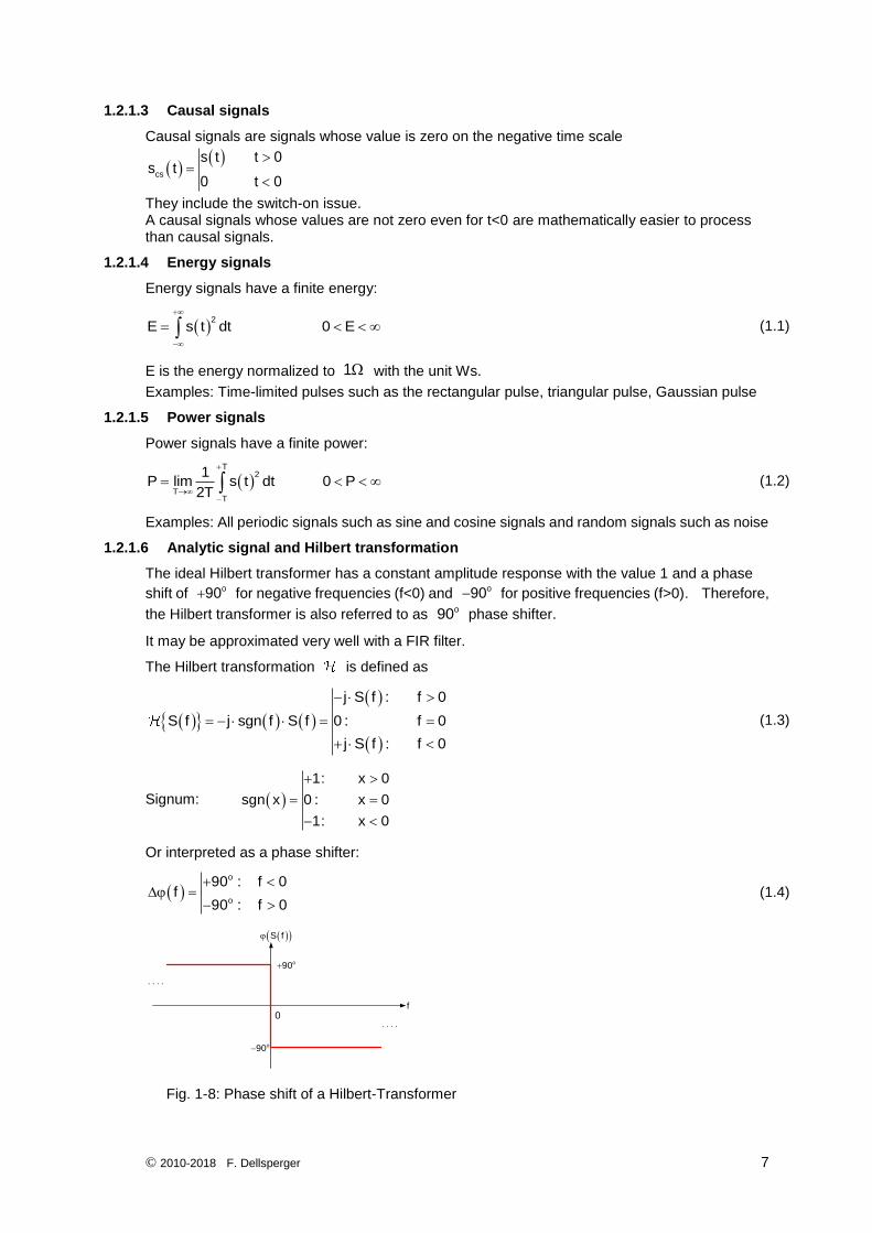
1.2.1.6 Analytic signal and Hilbert transformation
The ideal Hilbert transformer has a constant amplitude response with the value 1 and a phase
shift of o90 for negative frequencies (f<0) and o90 for positive frequencies (f>0). Therefore,
the Hilbert transformer is also referred to as o90 phase shifter.
It may be approximated very well with a FIR filter.
The Hilbert transformation is defined as
j S f : f 0
S f j sgn f S f 0 : f 0
j S f : f 0
(1.3)
Signum:
1: x 0
sgn x 0 : x 0
1: x 0
Or interpreted as a phase shifter:
o
o
90 : f 0f
90 : f 0
(1.4)
f0
S f
o90
o90
Fig. 1-8: Phase shift of a Hilbert-Transformer
© 2010-2018 F. Dellsperger 8
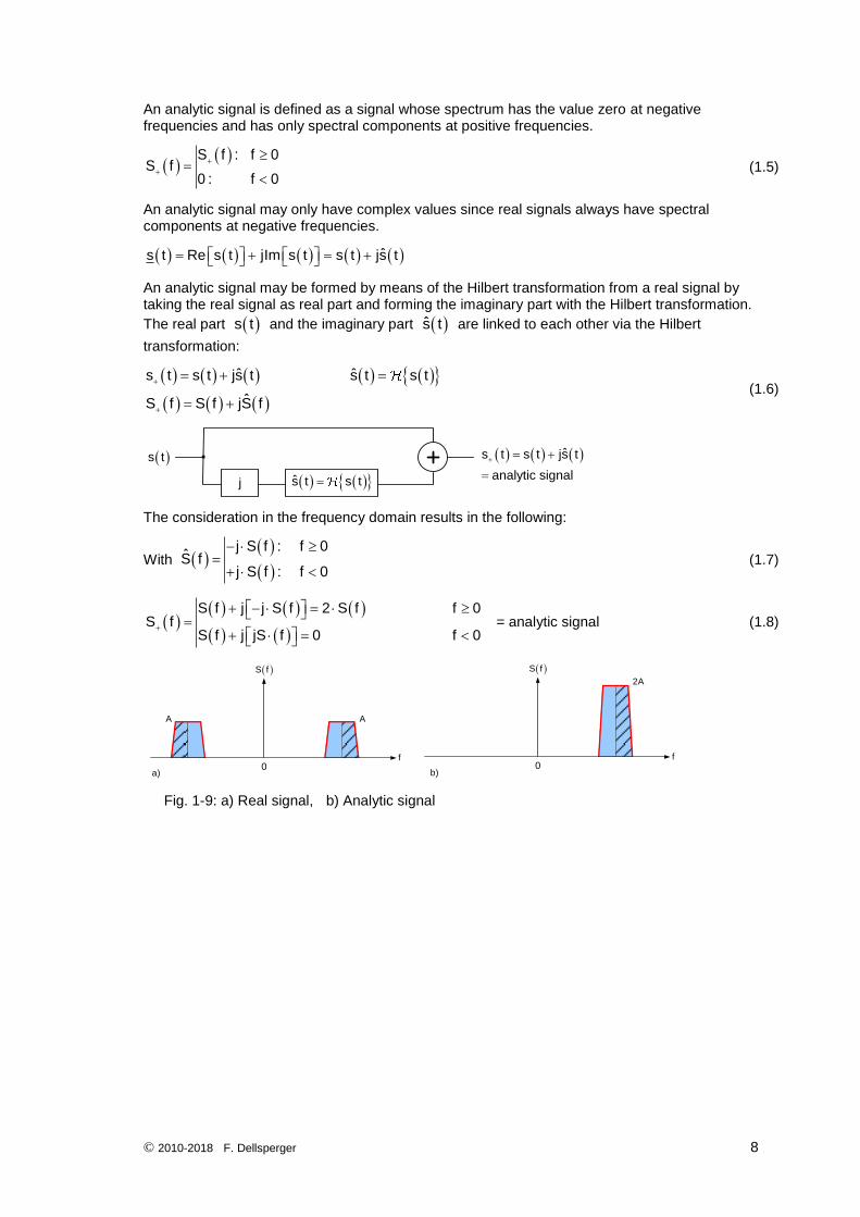
An analytic signal is defined as a signal whose spectrum has the value zero at negative frequencies and has only spectral components at positive frequencies.
S f : f 0
S f0 : f 0
(1.5)
An analytic signal may only have complex values since real signals always have spectral components at negative frequencies.
ˆs t Re s t jIm s t s t js t
An analytic signal may be formed by means of the Hilbert transformation from a real signal by taking the real signal as real part and forming the imaginary part with the Hilbert transformation.
The real part s t and the imaginary part s t are linked to each other via the Hilbert
transformation:
ˆ ˆs t s t js t s t s t
ˆS f S f jS f
(1.6)
s t s tj
ˆs t s t js t
analytic signal
s t
The consideration in the frequency domain results in the following:
With
j S f : f 0S f
j S f : f 0
(1.7)
S f j j S f 2 S f f 0S f
S f j jS f 0 f 0
= analytic signal (1.8)
f0
S f
f0
S f
AA
2A
a) b)
Fig. 1-9: a) Real signal, b) Analytic signal
© 2010-2018 F. Dellsperger 9
The following applies as well:
22
s t s t s t
= envelope (1.9)
s tt arctan
s t
= instantaneous phase (1.10)
d t1
f t2 dt
= instantaneous frequency (1.11)
1.2.1.7 Continuous signals
A continuous signal (analog signal) has continuous amplitude and a continuous time.
t
s t
0
Fig. 1-10: Continuous or analog signal
Examples: Microphone signals, sensor signals, sine and cosine signals
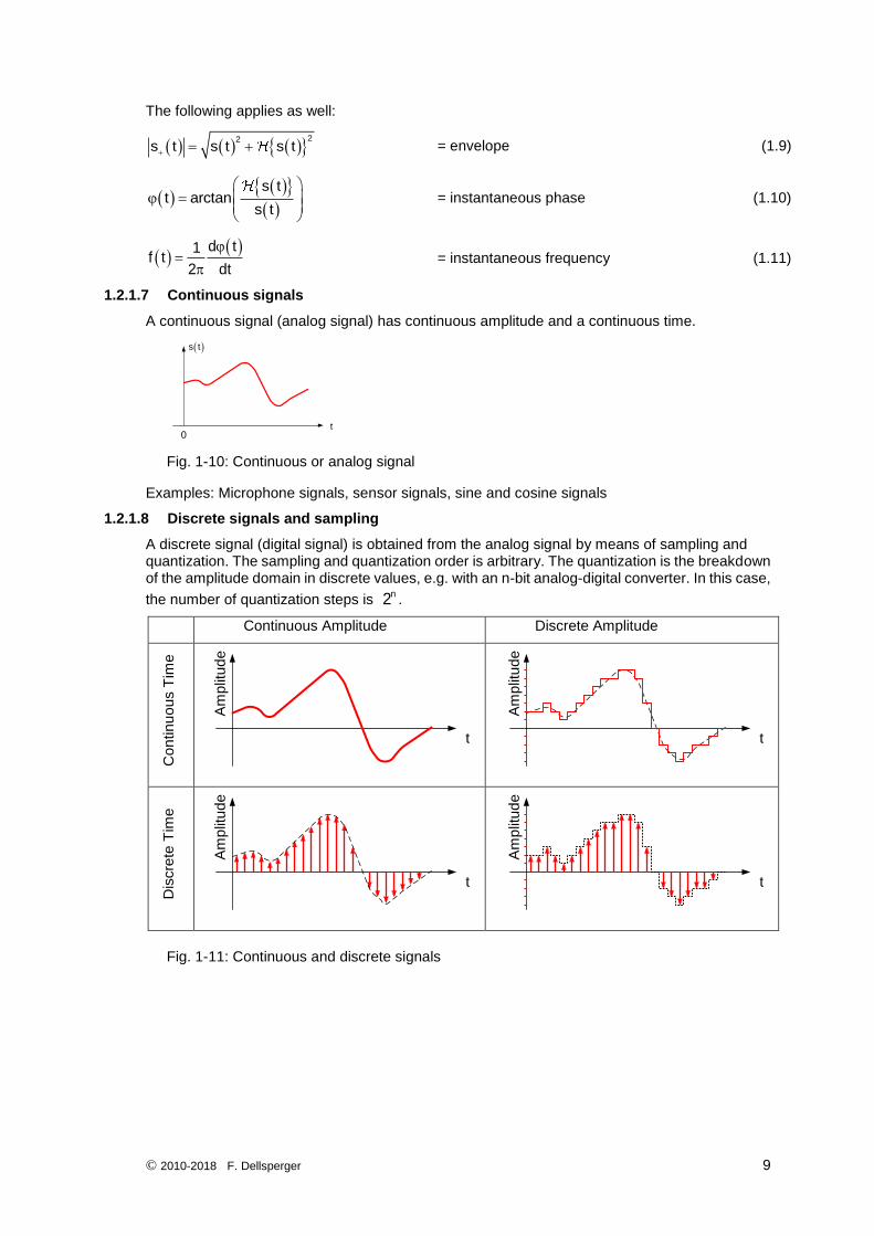
1.2.1.8 Discrete signals and sampling
A discrete signal (digital signal) is obtained from the analog signal by means of sampling and quantization. The sampling and quantization order is arbitrary. The quantization is the breakdown of the amplitude domain in discrete values, e.g. with an n-bit analog-digital converter. In this case,
the number of quantization steps is n2 .
Continuous Amplitude Discrete Amplitude
Co
ntin
uo
us T
ime
t
Am
plit
ud
e
t
Am
plit
ud
e
Dis
cre
te T
ime
t
Am
plit
ud
e
t
Am
plit
ud
e
Fig. 1-11: Continuous and discrete signals
© 2010-2018 F. Dellsperger 10
The ideal sampler multiplies the analog signal s(t) with the sampling function s t .
s s s s s
n n
s t s t t s t t nT s nT t nT
(1.12)
t
s t
t
s t
sT
Fig. 1-12: Analog signal and sampling function
sT is the sampling period and s sf 1/ T the sampling frequency or sampling rate.
The result is a value-continuous, time-discrete signal consisting of a Dirac pulse sequence whose
weights correspond to the sampling values s ss nT .
t
ss t
s ss nT
s t
Fig. 1-13: Sampled analog signal
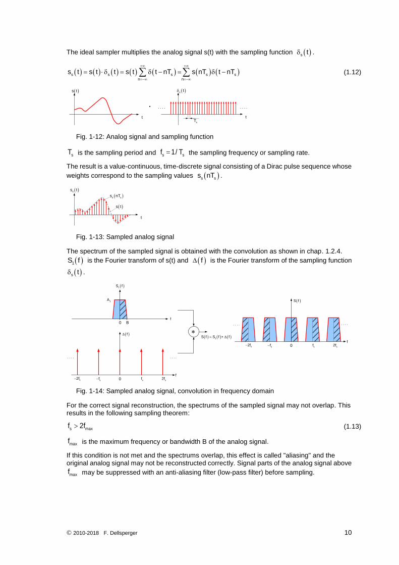
The spectrum of the sampled signal is obtained with the convolution as shown in chap. 1.2.4.
1S f is the Fourier transform of s(t) and f is the Fourier transform of the sampling function
s t .
f0 s2fsfs2f
sf
f
f0
1S f
1A
1S f S f f
f0 s2fsfs2f
sf
S f
B
Fig. 1-14: Sampled analog signal, convolution in frequency domain
For the correct signal reconstruction, the spectrums of the sampled signal may not overlap. This results in the following sampling theorem:
s maxf 2f (1.13)
maxf is the maximum frequency or bandwidth B of the analog signal.
If this condition is not met and the spectrums overlap, this effect is called "aliasing" and the original analog signal may not be reconstructed correctly. Signal parts of the analog signal above
maxf may be suppressed with an anti-aliasing filter (low-pass filter) before sampling.
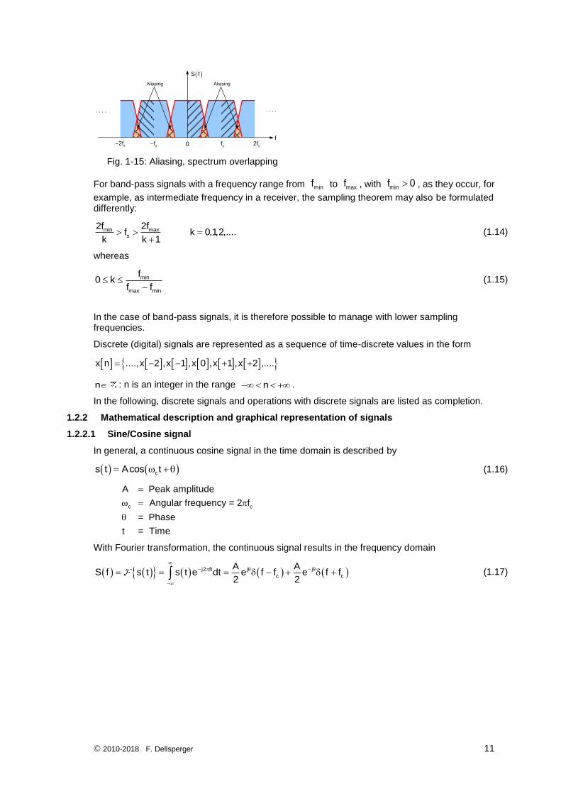
© 2010-2018 F. Dellsperger 11
f0 s2fsfs2f
sf
S f
AliasingAliasing
Fig. 1-15: Aliasing, spectrum overlapping
For band-pass signals with a frequency range from minf to maxf , with minf 0 , as they occur, for
example, as intermediate frequency in a receiver, the sampling theorem may also be formulated differently:
maxmins
2f2ff k 0,1,2,....
k k 1
(1.14)
whereas
min
max min
f0 k
f f
(1.15)
In the case of band-pass signals, it is therefore possible to manage with lower sampling frequencies.
Discrete (digital) signals are represented as a sequence of time-discrete values in the form
x n ....,x 2 ,x 1 ,x 0 ,x 1 ,x 2 ,....
n : n is an integer in the range n .
In the following, discrete signals and operations with discrete signals are listed as completion.
1.2.2 Mathematical description and graphical representation of signals
1.2.2.1 Sine/Cosine signal
In general, a continuous cosine signal in the time domain is described by
cs t Acos t (1.16)
c c
A Peak amplitude
Angular frequency = 2 f
= Phase
t = Time
With Fourier transformation, the continuous signal results in the frequency domain
j2 ft j j
c c
A AS f s t s t e dt e f f e f f
2 2
(1.17)
© 2010-2018 F. Dellsperger 12
A cosine carrier influenced by the modulation signal is described by
c c cˆs t V cos t
AM FM PMc
c c
V Carrier peak voltage
Carrier angular frequency = 2 f
= Carrier phase at t 0
t = Time
(1.18)
There are three options for influencing the carrier by means of the modulation signal:
c cV , ,
Amplitude modulation:
Amplitude modulation is modifying the carrier amplitude cV with the modulation content.
c and remain constant. is assumed to be 0 in most cases.
Frequency modulation:
Frequency modulation is modifying the carrier frequency c with the modulation content.
The carrier amplitude remains constant. Due to the relation t t dt , a frequency change
also results in a phase change.
Phase modulation:
Phase modulation is modifying the carrier phase with the modulation content.
The carrier amplitude remains constant. Due to the relation d t
tdt
, a phase change also
results in a frequency change.
Frequency and phase modulation are both covered by the term angle modulation. Both influence the argument (angle) of the cosine.
Representation options of the sine signal
For describing the signals, different representations may be used. The representations are explained with the cosine signal.
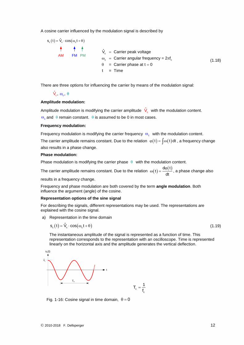
a) Representation in the time domain
c c cˆs t V cos t (1.19)
The instantaneous amplitude of the signal is represented as a function of time. This representation corresponds to the representation with an oscilloscope. Time is represented linearly on the horizontal axis and the amplitude generates the vertical deflection.
t
Tc
sc(t)
cV
c
c
1T
f
Fig. 1-16: Cosine signal in time domain, 0
© 2010-2018 F. Dellsperger 13
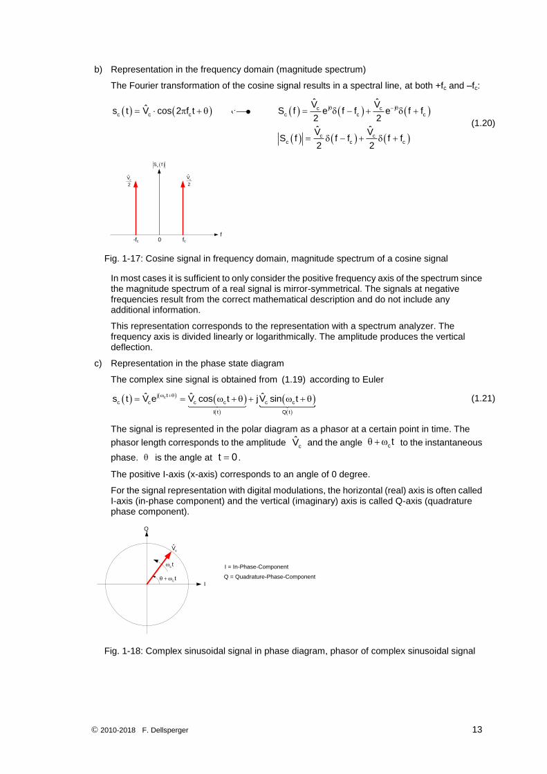
b) Representation in the frequency domain (magnitude spectrum)
The Fourier transformation of the cosine signal results in a spectral line, at both +fc and –fc:
j jc cc c c c c c
c cc c c
ˆ ˆV Vˆs t V cos 2 f t S f e f f e f f2 2
ˆ ˆV VS f f f f f
2 2
(1.20)
ffc0-fc
cS f
cV
2
cV
2
Fig. 1-17: Cosine signal in frequency domain, magnitude spectrum of a cosine signal
In most cases it is sufficient to only consider the positive frequency axis of the spectrum since the magnitude spectrum of a real signal is mirror-symmetrical. The signals at negative frequencies result from the correct mathematical description and do not include any additional information.
This representation corresponds to the representation with a spectrum analyzer. The frequency axis is divided linearly or logarithmically. The amplitude produces the vertical deflection.
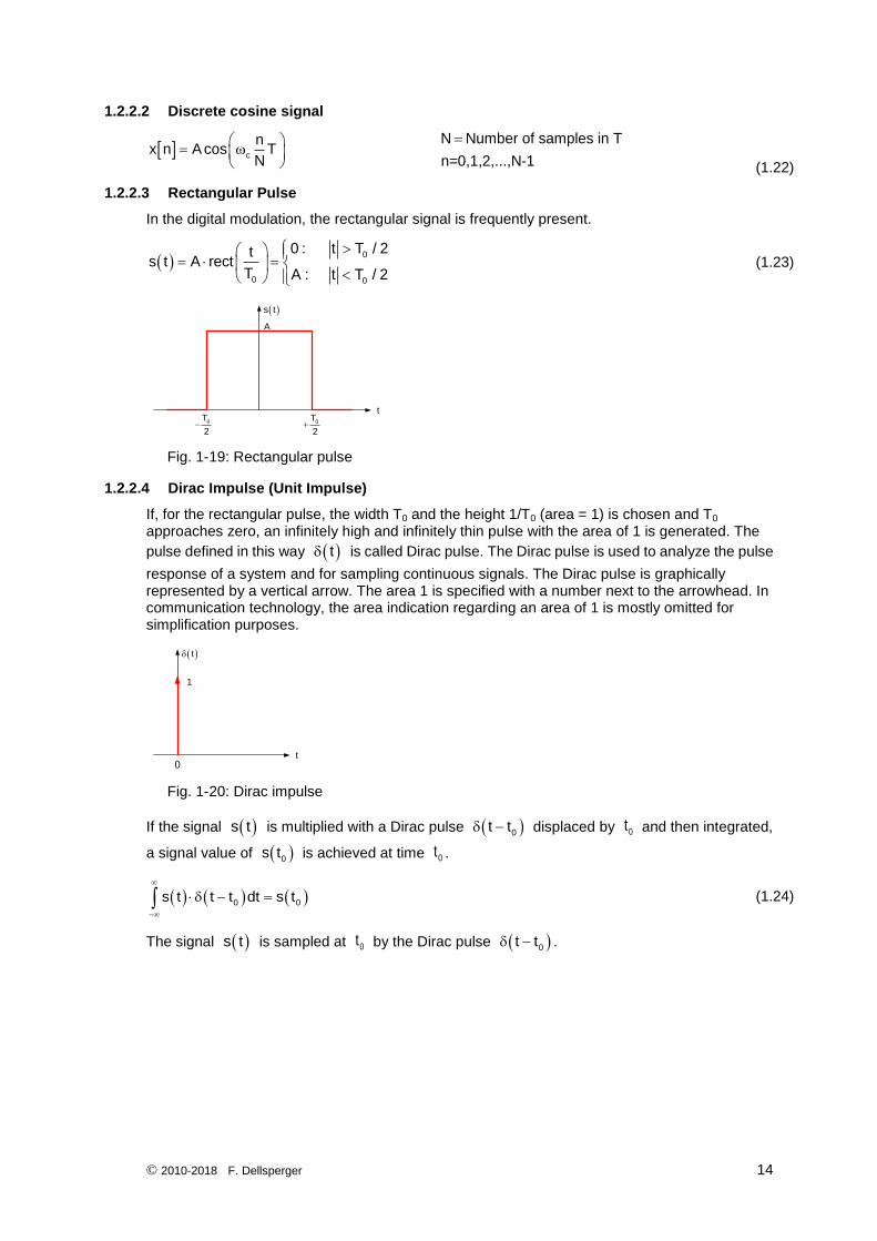
c) Representation in the phase state diagram
The complex sine signal is obtained from (1.19) according to Euler
cj t
c c c c c c
I t Q t
ˆ ˆ ˆs t V e V cos t jV sin t
(1.21)
The signal is represented in the polar diagram as a phasor at a certain point in time. The
phasor length corresponds to the amplitude cV and the angle c t to the instantaneous
phase. is the angle at t 0 .
The positive I-axis (x-axis) corresponds to an angle of 0 degree.
For the signal representation with digital modulations, the horizontal (real) axis is often called I-axis (in-phase component) and the vertical (imaginary) axis is called Q-axis (quadrature phase component).
I
Q
I = In-Phase-Component
Q = Quadrature-Phase-Component
c t
c t
cV
Fig. 1-18: Complex sinusoidal signal in phase diagram, phasor of complex sinusoidal signal
© 2010-2018 F. Dellsperger 14
1.2.2.2 Discrete cosine signal
c
nx n A cos T
N
N Number of samples in T
n=0,1,2,...,N-1
(1.22)
1.2.2.3 Rectangular Pulse
In the digital modulation, the rectangular signal is frequently present.
0
0 0
0 : t T / 2ts t A rect
T A : t T / 2
(1.23)
t
s t
0T
20T
2
A
Fig. 1-19: Rectangular pulse
1.2.2.4 Dirac Impulse (Unit Impulse)
If, for the rectangular pulse, the width T0 and the height 1/T0 (area = 1) is chosen and T0 approaches zero, an infinitely high and infinitely thin pulse with the area of 1 is generated. The
pulse defined in this way t is called Dirac pulse. The Dirac pulse is used to analyze the pulse
response of a system and for sampling continuous signals. The Dirac pulse is graphically represented by a vertical arrow. The area 1 is specified with a number next to the arrowhead. In communication technology, the area indication regarding an area of 1 is mostly omitted for simplification purposes.
t
t
1
0
Fig. 1-20: Dirac impulse
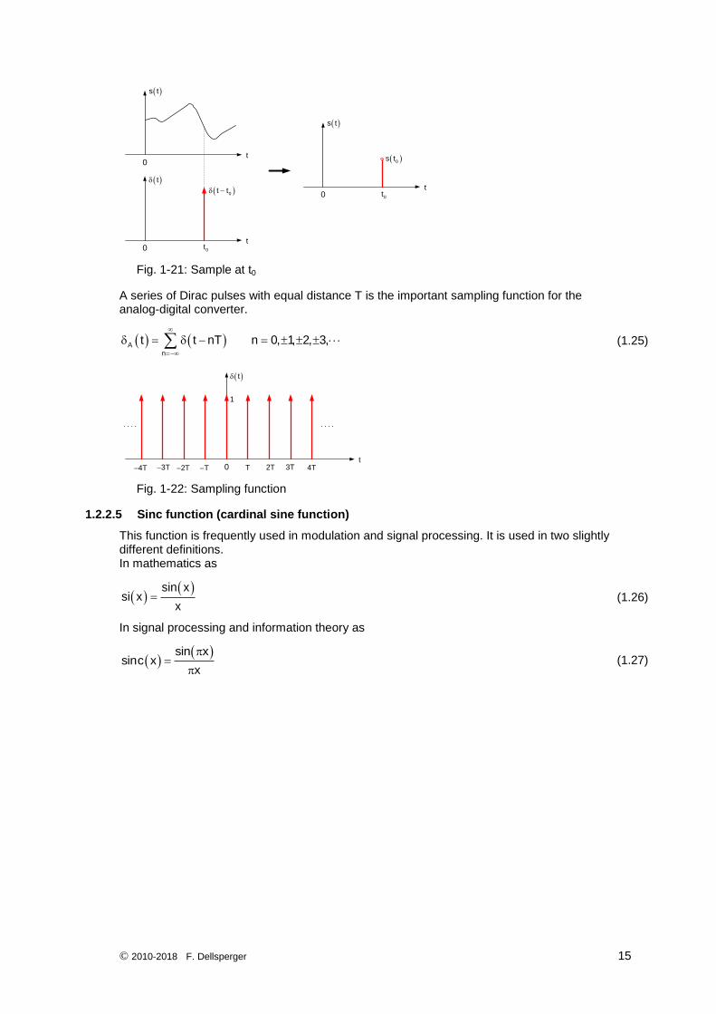
If the signal s t is multiplied with a Dirac pulse 0t t displaced by 0t and then integrated,
a signal value of 0s t is achieved at time 0t .
0 0s t t t dt s t
(1.24)
The signal s t is sampled at 0t by the Dirac pulse 0t t .
© 2010-2018 F. Dellsperger 15
t
s t
0
t
t
0
0t t
0t
t
s t
0
0s t
0t
Fig. 1-21: Sample at t0
A series of Dirac pulses with equal distance T is the important sampling function for the analog-digital converter.
A
n
t t nT n 0, 1, 2, 3,
(1.25)
t
t
1
0 2TT 3T 4T3T4T 2T T
Fig. 1-22: Sampling function
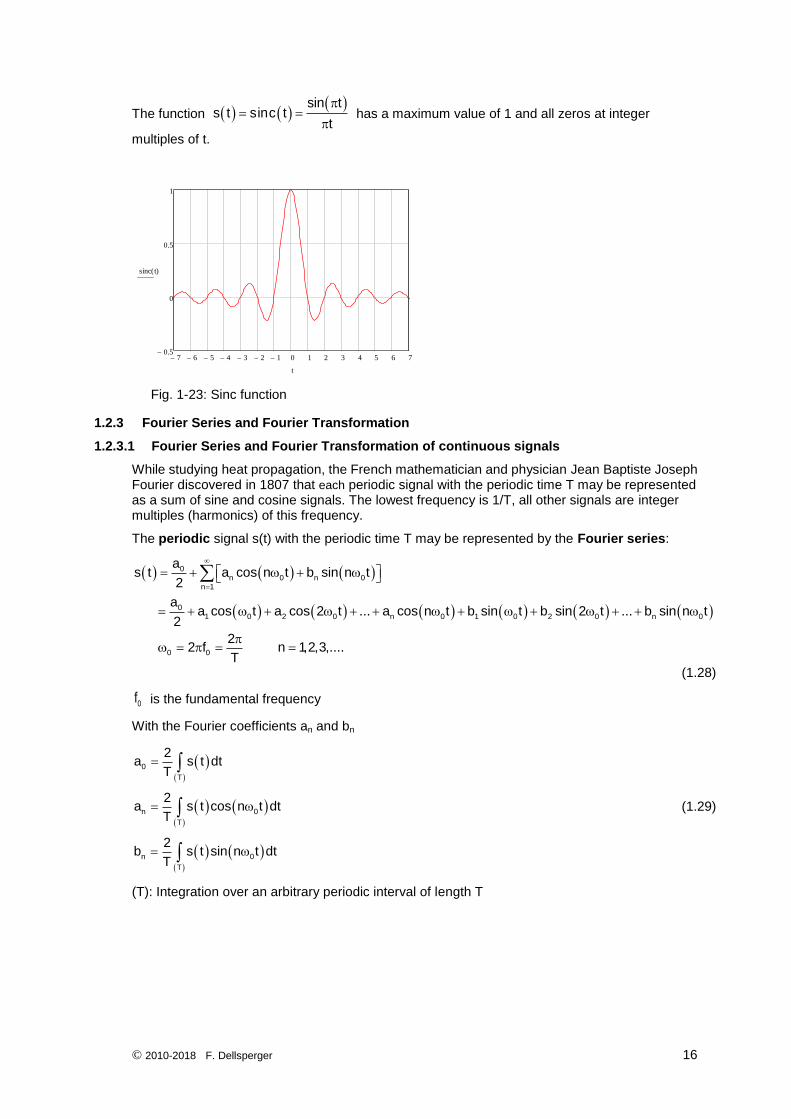
1.2.2.5 Sinc function (cardinal sine function)
This function is frequently used in modulation and signal processing. It is used in two slightly different definitions. In mathematics as
sin x
si xx
(1.26)
In signal processing and information theory as
sin x
sinc xx
(1.27)
© 2010-2018 F. Dellsperger 16
The function sin t
s t sinc tt
has a maximum value of 1 and all zeros at integer
multiples of t.
Fig. 1-23: Sinc function
1.2.3 Fourier Series and Fourier Transformation
1.2.3.1 Fourier Series and Fourier Transformation of continuous signals
While studying heat propagation, the French mathematician and physician Jean Baptiste Joseph Fourier discovered in 1807 that each periodic signal with the periodic time T may be represented as a sum of sine and cosine signals. The lowest frequency is 1/T, all other signals are integer multiples (harmonics) of this frequency.
The periodic signal s(t) with the periodic time T may be represented by the Fourier series:
0n 0 n 0
n 1
01 0 2 0 n 0 1 0 2 0 n 0
0 0
as t a cos n t b sin n t
2
aa cos t a cos 2 t ... a cos n t b sin t b sin 2 t ... b sin n t
2
22 f n 1,2,3,....
T
(1.28)
0f is the fundamental frequency
With the Fourier coefficients an and bn
0
T
n 0
T
n 0
T
2a s t dt
T
2a s t cos n t dt
T
2b s t sin n t dt
T
(1.29)
(T): Integration over an arbitrary periodic interval of length T
7 6 5 4 3 2 1 0 1 2 3 4 5 6 70.5
0
0.5
1
sinc t( )
t
© 2010-2018 F. Dellsperger 17
By combining the sine and cosine terms of the same frequency, an amplitude phase form is obtained.
n 0 n 0 n 0 na cos n t b sin n t A cos n t (1.30)
0 n 0 n 0 0 n 0 nn 1 n 1
0 1 0 1 2 0 2 n 0 n
s t A a cos n t b sin n t A A cos n t
A A cos t A cos 2 t .... A cos n t
(1.31)
With
00
2 2 th
n n n
thnn n
n
aA DC
2
A a b Amplitude of n Harmonic
barctan Phase of n Harmonic (+ if a 0)
a
(1.32)
For even functions s t s t :
0
T
n 0
T
n
2a s t dt
T
2a s t cos n t dt
T
b 0
(1.33)
For odd functions s t s t :
0
n
n 0
T
a 0
a 0
2b s t sin n t dt
T
(1.34)
With the relations
0 0 0 0jn t jn t jn t jn t
0 0
1 1cos n t e e sin n t e e
2 2j
the complex Fourier series with the complex Fourier coefficients cn is obtained:
0
0
jn t
nn
jn t *
n n n
T
0 0 n n n n
s t c e
1c s t e dt c c
T
A c A 2 c c
(1.35)

© 2010-2018 F. Dellsperger 18
For converting the coefficients, the following applies:
n n
0n
n n
1a jb : n 0
2
ac : n 0
2
1a jb : n 0
2
n n
n n
a 2Re c n 0
b 2Im c n 0
(1.36)
The periodic signal results in a line spectrum with spectral lines at 0 0 0 0f ,2f ,3f ....nf .
The power sP of a periodic signal normalized to a load resistance of 1 Ohm corresponds to the
sum of the powers of the individual harmonics (theorem of Parseval):
22 2 222 0n n n
s n 0 nN 0 n 1 n 1 n
aA a bP P A c
2 2 2
(1.37)
A non-periodic (aperiodic) signal s(t) may be described by means of the Fourier transformation in the frequency domain:
j2 ftS f s t s t e dt
(1.38)
And the inverse transformation in the time domain:
1 j2 fts t S f S f e df
(1.39)
S f and s t form a transformation pair, which is expressed with a symbol
s t S f
S f specifies the distribution of amplitude versus frequency. If s t has the unit of a voltage,
the Fourier transform S f has the unit Vs or V/Hz and represents an amplitude density.
An aperiodic signal has a continuous amplitude density spectrum.
The Fourier transform S f is a complex function and may be represented as a real and
imaginary part or magnitude and phase:
j fS f Re S f jIm S f S f e
With
2 2Im S f
S f Re S f Im S f f arctanRe S f
(1.40)
© 2010-2018 F. Dellsperger 19
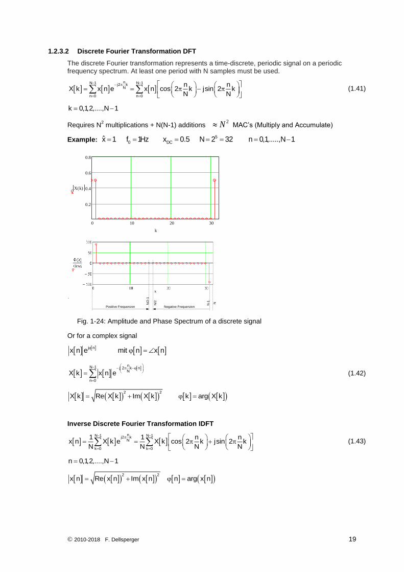
1.2.3.2 Discrete Fourier Transformation DFT
The discrete Fourier transformation represents a time-discrete, periodic signal on a periodic frequency spectrum. At least one period with N samples must be used.
nN 1 N 1j2 kN
n 0 n 0
n nX k x n e x n cos 2 k jsin 2 k
N N
(1.41)
k 0,1,2,....,N 1
Requires N2 multiplications + N(N-1) additions
2N MAC’s (Multiply and Accumulate)
Example: 5
0 DCx 1 f 1Hz x 0.5 N 2 32 n 0,1,.....,N 1
0 10 20 30
0.2
0.4
0.6
0.8
X k( )
k
N/2
-1
N/2
N-1 N
Positive Frequenzen Negative Frequenzen
k
Fig. 1-24: Amplitude and Phase Spectrum of a discrete signal
Or for a complex signal
j nx n e mit n x n
nN 1 j 2 k nN
n 0
X k x n e
(1.42)
2 2
X k Re X k Im X k k arg X k
Inverse Discrete Fourier Transformation IDFT
nN 1 N 1j2 kN
k 0 k 0
1 1 n nx n X k e X k cos 2 k jsin 2 k
N N N N
(1.43)
n 0,1,2,....,N 1
2 2
x n Re x n Im x n n arg x n
© 2010-2018 F. Dellsperger 20
Fast Fourier Transformation FFT and IFFT
FFT and IFFT are special algorithms for calculating the discrete Fourier transformation and requires significantly less computer resources than DFT and IDFT.
Condition: qN 2 q 1,2,.....
Requires 2N
N2 MAC’s (Multiply and Accumulate)
1.2.3.3 Examples:
Periodic unipolar square wave
t
s t
sT
2sT
2
A
0T 0T
sT
f
A
2
0
03f
0f 05f05f
03f
0f
S f
1 2A
2
1 2A
2 3
1 2A
2 5
f
A
2
0 03f0f 05f05f03f 0f
S f
1 2A
2
1 2A
2 3
1 2A
2 5
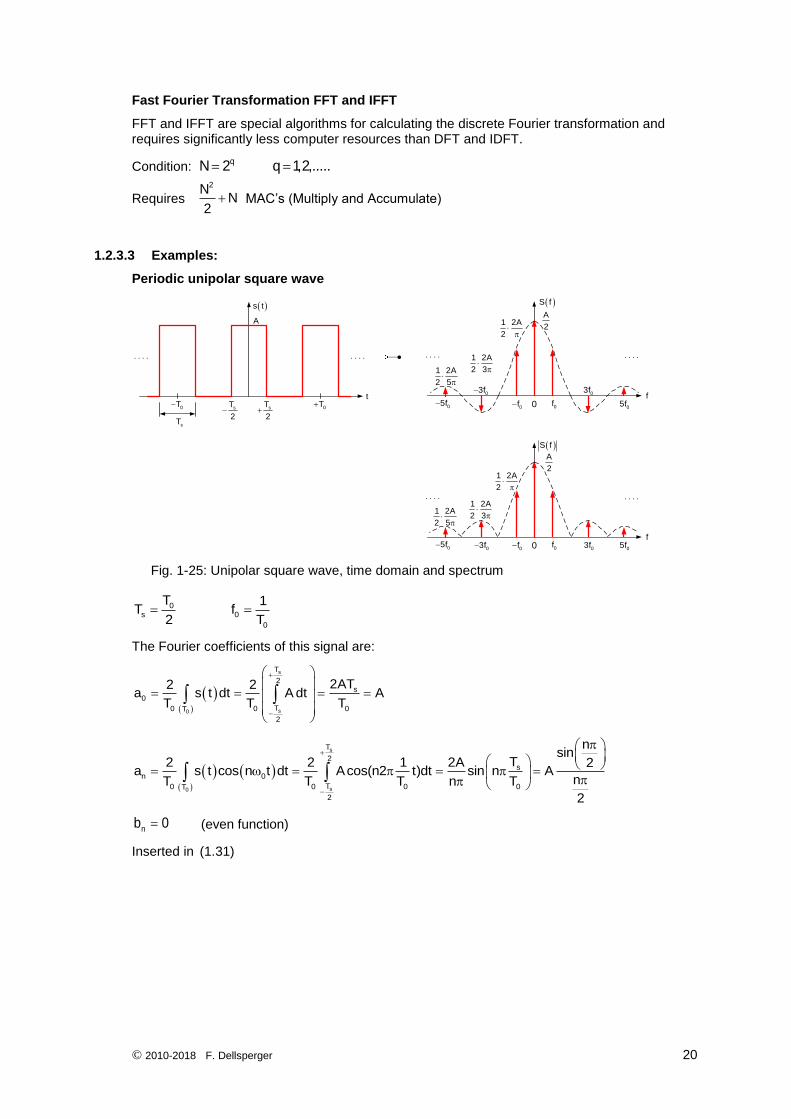
Fig. 1-25: Unipolar square wave, time domain and spectrum
0s 0
0
T 1T f
2 T
The Fourier coefficients of this signal are:
s
s0
T
2s
0
T0 0 0T
2
2AT2 2a s t dt A dt A
T T T
s
s0
T
2s
n 0
T0 0 0 0T
2
nsin
T2 2 1 2A 2a s t cos n t dt Acos(n2 t)dt sin n A
nT T T n T
2
nb 0 (even function)
Inserted in (1.31)
© 2010-2018 F. Dellsperger 21
0 n 0 n n 0 0n 1 n 1 n 1
0 0 0
nsin
A A 2s t A A cos n t a cos n2 f t A cos n2 f t
n2 2
2
A 2A 1 1cos 2 f t cos 2 3f t cos 2 5f t ....
2 3 5
The spectrum of the ideal square wave with a duty cycle of 1:1 ( s 0T T / 2 ) has only odd
harmonics. Their amplitudes have a behavior proportional to 1/ n .
The envelope of the amplitudes of the spectral lines follows the sinc function
nsin
2
n
2
.
The zeros are at even harmonics.
The fundamental frequency 0f is also called the 1st harmonic.
0.6 0.8 1 1.2 1.40.5
0
0.5
1
1.5
t
s(t)
N=5 3 11
9%
s t
t
0.6 0.8 1 1.2 1.40.5
0
0.5
1
1.5
t
s(t) s t
t
N=99
N: Number of Harmonics
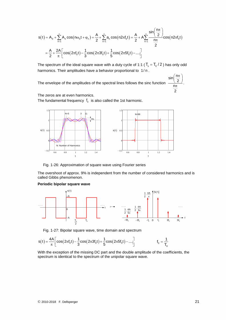
Fig. 1-26: Approximation of square wave using Fourier series
The overshoot of approx. 9% is independent from the number of considered harmonics and is called Gibbs phenomenon.
Periodic bipolar square wave
t
s t
0T
2
A
0T
f0 03f0f 05f05f
03f 0f
S f1 4A
2
1 4A
2 3
1 4A
2 5
0
A
Fig. 1-27: Bipolar square wave, time domain and spectrum
0 0 0
4A 1 1s t cos 2 f t cos 2 3f t cos 2 5f t ....
3 5
0
0
1f
T
With the exception of the missing DC part and the double amplitude of the coefficients, the spectrum is identical to the spectrum of the unipolar square wave.
© 2010-2018 F. Dellsperger 22
Periodic unipolar pulse train
t
s t
A
0T 0T
f
0
A
T
0 03f0f 04f04f03f 0f
S f
0
1 2A nsin
2 n T
02f02f
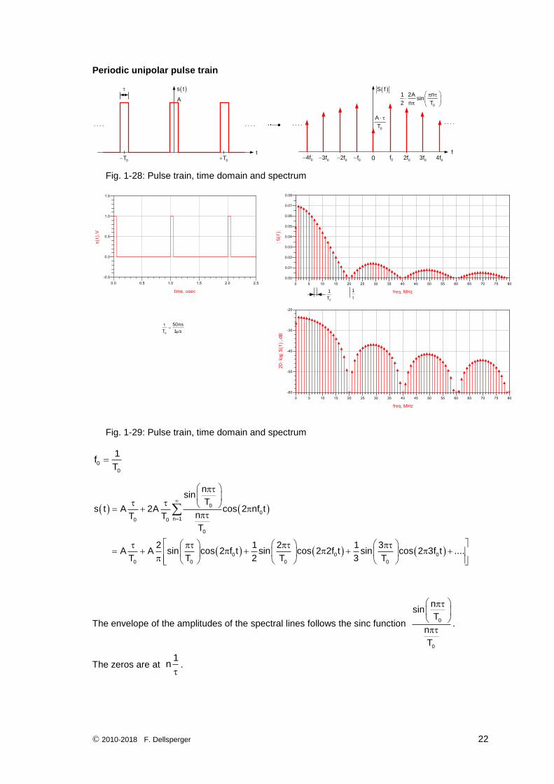
Fig. 1-28: Pulse train, time domain and spectrum
Sf
st
,V
0
1
T
1
20
log
Sf
,dB
0
50ns
T 1 s
Fig. 1-29: Pulse train, time domain and spectrum
0
0
1f
T
0
0n 10 0
0
0 0 0
0 0 0 0
nsin
Ts t A 2A cos 2 nf t
nT T
T
2 1 2 1 3A A sin cos 2 f t sin cos 2 2f t sin cos 2 3f t ....
T T 2 T 3 T
The envelope of the amplitudes of the spectral lines follows the sinc function 0
0
nsin
T
n
T
.
The zeros are at 1
n
.
© 2010-2018 F. Dellsperger 23
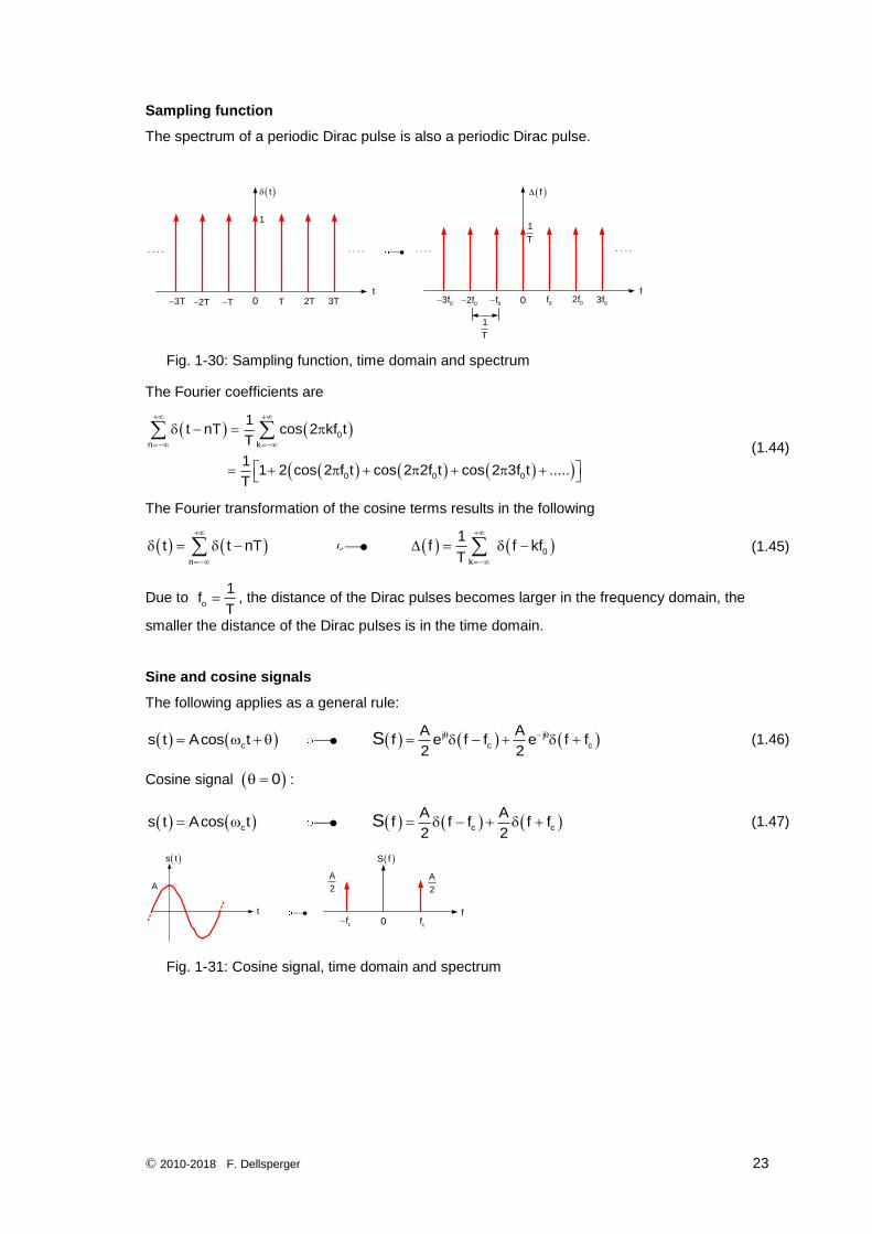
Sampling function
The spectrum of a periodic Dirac pulse is also a periodic Dirac pulse.
t
t
1
0 2TT 3T3T 2T T
f
1
T
0 02f0f 03f
03f02f 0f
f
1
T
Fig. 1-30: Sampling function, time domain and spectrum
The Fourier coefficients are
0
n k
0 0 0
1t nT cos 2 kf t
T
11 2 cos 2 f t cos 2 2f t cos 2 3f t .....
T
(1.44)
The Fourier transformation of the cosine terms results in the following
0
n k
1t t nT f f kf
T
(1.45)
Due to o
1f
T , the distance of the Dirac pulses becomes larger in the frequency domain, the
smaller the distance of the Dirac pulses is in the time domain.
Sine and cosine signals
The following applies as a general rule:
j j
c c c
A As t Acos t f e f f e f f
2 2S (1.46)
Cosine signal 0 :
c c c
A As t Acos t f f f f f
2 2S (1.47)
s t
A
t f0 cfcf
S f
A
2
A
2
Fig. 1-31: Cosine signal, time domain and spectrum
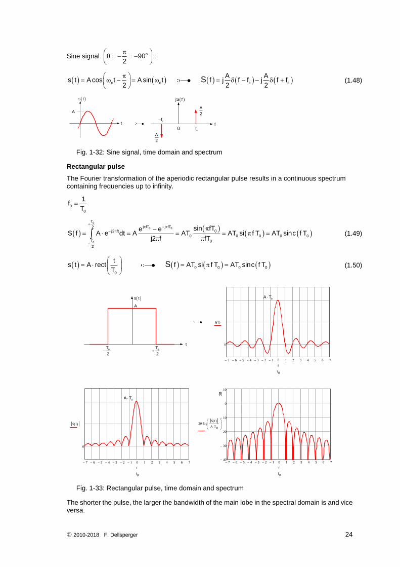
© 2010-2018 F. Dellsperger 24
Sine signal o902
:
c c c c
A As t Acos t A sin t f j f f j f f
2 2 2S
(1.48)
s t
A
t f0 cf
cf
jS f
A
2
A
2
Fig. 1-32: Sine signal, time domain and spectrum
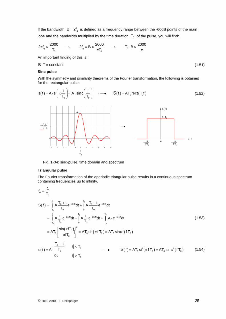
Rectangular pulse
The Fourier transformation of the aperiodic rectangular pulse results in a continuous spectrum containing frequencies up to infinity.
0
0
1f
T
0
0 0
0
T
j fT j fT20j2 ft
0 0 0 0 0
T 0
2
sin fTe eS f A e dt A AT AT si f T AT sinc f T
j2 f fT
(1.49)
0 0 0 0
0
ts t A rect f AT si f T AT sinc f T
TS
(1.50)
t
s t
0T
20T
2
A
0A T
0A T
7 6 5 4 3 2 1 0 1 2 3 4 5 6 7
0
0.5
1
S f( )
f
f0
7 6 5 4 3 2 1 0 1 2 3 4 5 6 7
0
0.5
1
S f( )
f
f0
7 6 5 4 3 2 1 0 1 2 3 4 5 6 740
30
20
10
0
10
20 logS f( )
A T0
f
f0
dB
Fig. 1-33: Rectangular pulse, time domain and spectrum
The shorter the pulse, the larger the bandwidth of the main lobe in the spectral domain is and vice versa.
© 2010-2018 F. Dellsperger 25
If the bandwidth gB 2f is defined as a frequency range between the -60dB points of the main
lobe and the bandwidth multiplied by the time duration 0T of the pulse, you will find:
g g 0
0 0
2000 2000 20002 f 2f B T B
T T
An important finding of this is:
B T constant (1.51)
Sinc pulse
With the symmetry and similarity theorems of the Fourier transformation, the following is obtained for the rectangular pulse:
0 0
0 0
t ts t A si A sinc f AT rect T f
T TS
(1.52)
5 4 3 2 1 0 1 2 3 4 5
0
0.5
1
sinct
T0
t
T0
A
f
S f
0
1
2T
0
1
2T
0A T
0
Fig. 1-34: sinc-pulse, time domain and spectrum
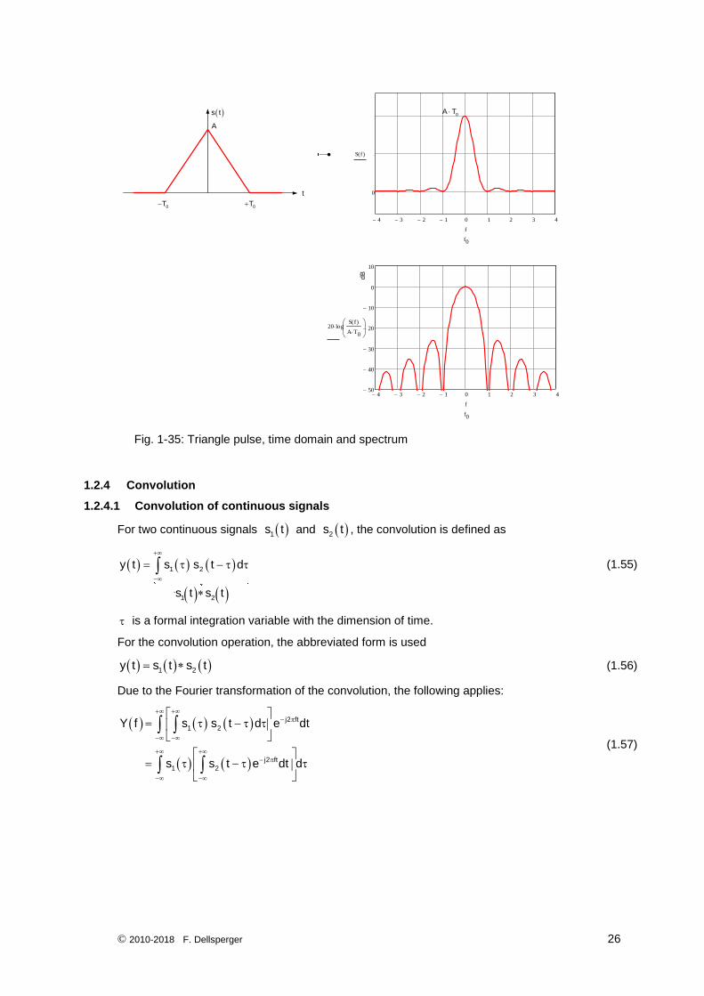
Triangular pulse
The Fourier transformation of the aperiodic triangular pulse results in a continuous spectrum containing frequencies up to infinity.
0
0
1f
T
0
0
0 0
0 0
T0
j2 ft j2 ft0 0
0 0T 0
T T0
j2 ft j2 ft j2 ft
0 0T 0 T
2
0 2 2
0 0 0 0 0
0
T t T tS f A e dt A e dt
T T
t tA e dt A e dt A e dt
T T
sin fTAT AT si f T AT sinc f T
fT
(1.53)
0
0 2 20 0 0 0 0
0
T t: t T
Ts t A f AT si f T AT sinc f T
0 : t T
S
(1.54)
© 2010-2018 F. Dellsperger 26
t
s t
0T0T
A
4 3 2 1 0 1 2 3 4
0
0.5
1
S f( )
f
f0
0A T
4 3 2 1 0 1 2 3 450
40
30
20
10
0
10
20 logS f( )
A T0
f
f0
dB
Fig. 1-35: Triangle pulse, time domain and spectrum
1.2.4 Convolution
1.2.4.1 Convolution of continuous signals
For two continuous signals 1s t and 2s t , the convolution is defined as
1 2
`1 2
y t s s t d
s t s t
(1.55)
is a formal integration variable with the dimension of time.
For the convolution operation, the abbreviated form is used
1 2y t s t s t (1.56)
Due to the Fourier transformation of the convolution, the following applies:
j2 ft
1 2
j2 ft
1 2
Y f s s t d e dt
s s t e dt d
(1.57)
© 2010-2018 F. Dellsperger 27
The term in the square brackets is the Fourier transformation of the signal 1s t delayed by
and therefore according to the time delay theorem j2 f
2S f e .
j2 f
1 2
j2 f
2 1
1
Y f s S f e d
S f s e d
S f
(1.58)
Thus,
1 2Y f S f S f
1 2 1 2s t s t f fS S (1.59)
and with the duality
1 2 1 2s t s t f fS S (1.60)
The convolution theorem specifies that the normal product and the convolution product of two functions form a Fourier transformation pair.
The product of two time functions results in the convolution of the two associated spectrums and vice versa.
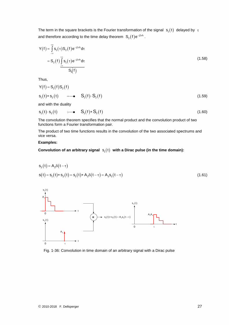
Examples:
Convolution of an arbitrary signal 1s t with a Dirac pulse (in the time domain):
2 2s t A t
1 2 1 2 2 1s t s t s t s t A t A s t (1.61)
t0
1s t
t0
2s t
2A
1A
t0
2s t
1 2A A
1 2 2 1s t s t A s t
Fig. 1-36: Convolution in time domain of an arbitrary signal with a Dirac pulse
© 2010-2018 F. Dellsperger 28
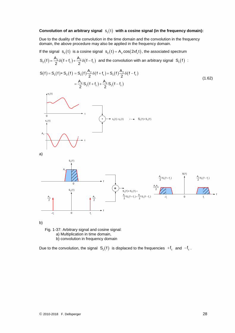
Convolution of an arbitrary signal 1s t with a cosine signal (in the frequency domain):
Due to the duality of the convolution in the time domain and the convolution in the frequency domain, the above procedure may also be applied in the frequency domain.
If the signal 2s t is a cosine signal 2 2 cs t A cos 2 f t , the associated spectrum
2 22 c c
A AS f f f f f
2 2 and the convolution with an arbitrary signal 1S f :
2 21 2 1 c 1 c
2 21 c 1 c
A AS f S f S f S f f f S f f f
2 2
A AS f f S f f
2 2
(1.62)
t
1s t
0
2s t
2A
t
1 2 1 2s t s t f S fS
a)
f0
1S f
f0
cfcf
2S f
f0
cfcf
S f
1A
2A
2
2A
2
1 2
2 21 c 1 c
S f S f
A AS f f S f f
2 2
1 2A A
2
21 c
AS f f
2 2
1 c
AS f f
2
b)
Fig. 1-37: Arbitrary signal and cosine signal: a) Multiplication in time domain, b) convolution in frequency domain
Due to the convolution, the signal 1S f is displaced to the frequencies cf and cf .
© 2010-2018 F. Dellsperger 29
Interpretation:
If an arbitrary signal 1s t is multiplied with a cosine signal 2s t in the time domain, a
convolution of the spectrums 1S f and 2S f is performed in the frequency domain. The
result is
A frequency displacement of the signal 1S f to the frequencies cf and cf
A double side band amplitude modulation with suppressed carrier
( 1s t =modulation signal, 2s t = carrier)
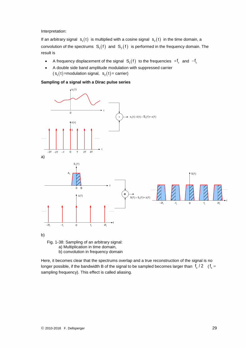
Sampling of a signal with a Dirac pulse series
t
1s t
0
t
t
1
0 2TT 3T3T 2T T
1 1s t t f fS
a)
f0 s2fsfs2f
sf
f
f0
1S f
1A
1S f S f f
f0 s2fsfs2f
sf
S f
B
b)
Fig. 1-38: Sampling of an arbitrary signal: a) Multiplication in time domain, b) convolution in frequency domain
Here, it becomes clear that the spectrums overlap and a true reconstruction of the signal is no
longer possible, if the bandwidth B of the signal to be sampled becomes larger than sf / 2 ( sf
sampling frequency). This effect is called aliasing.

© 2010-2018 F. Dellsperger 30
1.2.4.2 Convolution of discrete signals
2 discrete signals x n and h n
i
y n x i h n i x n h n
(1.63)
h n x n H k X k
h n x n H k X k
(1.64)
1.2.5 Correlation
Correlation is an operation which is used in modulation technology for the determination of the power spectral density of a signal and for the comparison of digital codes (e.g. for CDMA). It is closely related to the convolution.
For energy signals the correlation is defined as:
xy 1 2R s t s t dt
(1.65)
and for power signals
T/2
xy 1 2T
T/2
1R lim s t s t dt
T
(1.66)
The correlation function xyR represents a measure for the similarity or relation of both signals
1s t and 2s t in function of the displacement time . is the displacement time by means
of which the second signal 2s t is shifted to the left hand ( 0 ) or to the right hand side ( 0
) in respect to the first signal 1s t .
For periodic power signals with the periodic time 0T , the following applies
0T
xy 1 2
0 0
1R s t s t dt
T (1.67)
xyR is a periodic function as well provided that 0T applies to 1s t and 2s t .
If 1s t and 2s t are two different signals, a cross-correlation function (CCF) is given.
If 1 2s t s t s t a signal is correlated with itself which is called auto-correlation function
(ACF):
T/2
xxT
T/2
1R lim s t s t dt
T
(1.68)
In practice, it is necessary to set a limited time interval T with the result
T/2
xx
T/2
1R s t s t dt
T
(1.69)
© 2010-2018 F. Dellsperger 31
Or for a periodic power signal with the periodic time 0T
0T
xx
0 0
1R s t s t dt
T (1.70)
Characteristics of xxR :
xx xxmax: 0 R 0 R P
P = signal power, xxmaxR = maximum value of the ACF
xx xxR R (even function)
And for a periodic signal
xx 0 xx 0 xxR T R nT R 0 n 1,2,3,...
For discrete signals, for example, binary random bit sequences (PN codes), the correlation function may be determined with
P 1
xy k k vk 0
P 1
xx k k vk 0
1R v a b
P
1R v a a
P
(1.71)
k ka ,b = sequences of bits
k = bit number = 0,1,2,…P-1 P = number of bits of a period of the bit sequence = length of the PN code v = displacement in bits
Example of a PN code with the length 7:
k
1a
1
k 0 1 2 3 4 5 6 v P 1
k 0
xxR v
ka
+1 -1 -1 +1 -1 +1 +1
k 0a
+1 -1 -1 +1 -1 +1 +1 0 +7 +1.0
k 1a
+1 +1 -1 -1 +1 -1 +1 1 -1 -1/7
k 2a
+1 +1 +1 -1 -1 +1 -1 2 -1 -1/7
k va
… … … … … … … … … …
k 6a
-1 -1 +1 -1 +1 +1 +1 6 -1 -1/7
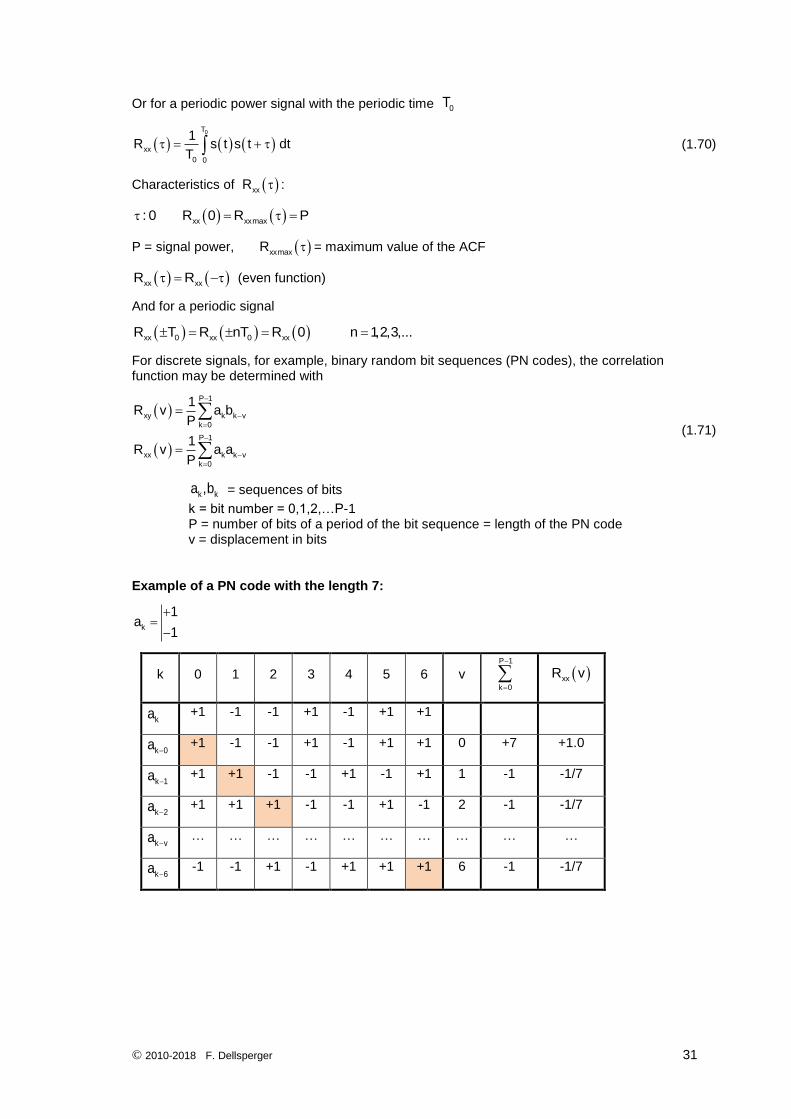
© 2010-2018 F. Dellsperger 32
v
1/ 7
xxR v
2 4 868 6 24
1
Fig. 1-39: Autocorrelation function of a PN-Code with length 7
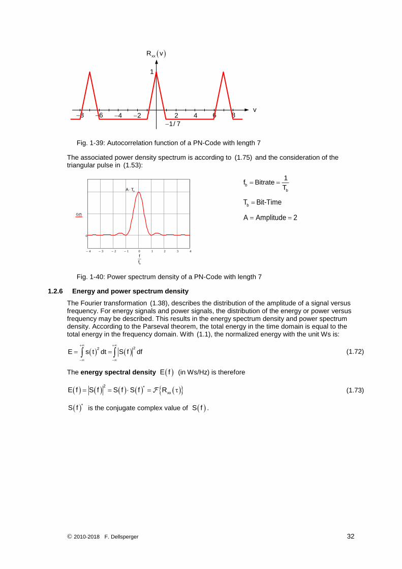
The associated power density spectrum is according to (1.75) and the consideration of the triangular pulse in (1.53):
4 3 2 1 0 1 2 3 4
0
0.5
1
S f( )
f
f0
bA T
G(f)
b
f
f
b
b
1f Bitrate
T
bT Bit-Time
A Amplitude 2
Fig. 1-40: Power spectrum density of a PN-Code with length 7
1.2.6 Energy and power spectrum density
The Fourier transformation (1.38), describes the distribution of the amplitude of a signal versus frequency. For energy signals and power signals, the distribution of the energy or power versus frequency may be described. This results in the energy spectrum density and power spectrum density. According to the Parseval theorem, the total energy in the time domain is equal to the total energy in the frequency domain. With (1.1), the normalized energy with the unit Ws is:
22
E s t dt S f df
(1.72)
The energy spectral density E f (in Ws/Hz) is therefore
2
xxE f S f S f S f R
(1.73)
S f is the conjugate complex value of S f .
© 2010-2018 F. Dellsperger 33
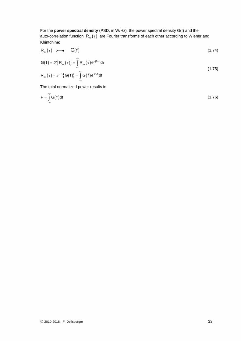
For the power spectral density (PSD, in W/Hz), the power spectral density G(f) and the
auto-correlation function xxR are Fourier transforms of each other according to Wiener and
Khintchine:
xxR fG (1.74)
j2 f
xx xx
1 j2 f
xx
G f R R e d
R G f G f e df
(1.75)
The total normalized power results in
P G f df
(1.76)
© 2010-2018 F. Dellsperger 34
1.3 References
[1] Taub, H., Schilling, D.L.: Principles of communication systems. McGraw-Hill, 2nd Edition 1986
[2] Kammeyer, K.D. : Nachrichtenübertragung. Vieweg+Teubner, 4. Auflage 2008
[3] Roppel, C.: Grundlagen der digitalen Kommunikationstechnik. Carl Hanser Verlag, 2006
[4] Ohm, J-R., Lüke, H.D.:Signalübertragung. Springer Verlag Berlin, 10. Auflage 2007
[5] Schwartz, M.: Information, Transmission, Modulation, and Noise. McGraw-Hill, 1980
[6] Zinke, O., Brunswig, H.: Hochfrequenztechnik 2, Springer Verlag Berlin, 5. Auflage 1999
[7] Stumpers, F.L.M.H.: Theory of frequency modulation noise. Proc. Inst. Radio Engrs. 36, 1948, 1081-1092
[8] Rice, S.O. : Statistical properties of a sine wave plus random noise. Bell Syst. Techn.J. 27, 1948, 109-157
[9] von Grünigen, D.Ch.: Digitale Signalerarbeitung mit einer Einführung in die kontinuierlichen Signale und Systeme. Carl Hanser Verlag, 5. Auflage 2014
[10] von Grünigen, D.Ch.: Digitale Signalerarbeitung: Bausteine, Systeme, Anwendungen. Fotorotar Print und Media, 2008
[11] Dellsperger, F.: Passive Filter der Hochfrequenz- und Nachrichtentechnik. Lecture Script, 2012