Embed Size (px)
Citation preview
Module 1: RelationsSection 1: Review of Mathematics 11
Lesson 1 Graphing Calculator Review 5
Lesson 2 Functions and Interval Notation 15
Lesson 3 Inverse Functions 24
Lesson 4 Polynomial Functions and Their Graphs 31
Review 45
Section Assignment 1.1 47
Section 2: Transformations
Lesson 1 Translations 59
Lesson 2 Reflections 69
Lesson 3 Absolute Value Functions 81
Lesson 4 Stretches and Compressions 89
Lesson 5 Reciprocal Relations 103
Lesson 6 Composition of Transformations 113
Summary 121
Review 123
Section Assignment 1.2 127
Module 1: Answer Key 137
Principles of Mathematics 12 Contents 1
Module 1

2 Contents Principles of Mathematics 12
Module 1
Module 1
Module 1, Section 1
Review of Mathematics 11
Introduction
In this section you will review a number of the concepts andprocesses encountered at the end of Principles of Math 11. Most ofthese concepts deal with functions and coordinate geometry. A solidfoundation of polynomials and rational functions is necessary tomaster transformations, which you will encounter in Sections 2 and 3 of this module and also in Modules 2 and 3.
Section 1 — Outline
Lesson 1 Graphing Calculator Review
Lesson 2 Functions and Interval Notation
Lesson 3 Inverse Functions
Lesson 4 Polynomial Functions and Their Graphs
Review
Principles of Mathematics 12 Section 1, Introduction 3

Notes
4 Section 1, Introduction Principles of Mathematics 12
Module 1
Module 1
Lesson 1
GRAPHING CALCULATOR REVIEW
Outcomes
Upon completing this lesson, you will be able to carry out theseoperations on a graphing calculator:
• Enter and edit polynomial equations
• Graph the equations and adjust the viewing window
• Solve the equations
Overview
If you used a graphing calculator for Principles of Math 11, thenconsider this lesson optional. You should do just a few of theexercises to make sure you remember how the graphing and solvingfunctions work.
The directions here are specific to the TI-83 or TI-83Plus modelsfrom Texas Instruments. You may be using a different TI model, orone made by Hewlett-Packard, Sharp, Casio, or anothermanufacturer. Any graphing calculator will get you through theprovincial exam (except the HP-48, which is not allowed). But if youuse another brand of calculator, you will need to refer to its usermanual to find out how to do what these instructions tell you.
Principles of Mathematics 12 Section 1, Lesson 1 5
Q: Can I use an ordinary scientific calculator for the exams in thiscourse and for the Provincial exam?
A: Not much. You are allowed to bring one to exams if you want to,but it’s not enough. The calculator you bring to the Provincialexam must be able to display graphs in its display window, aswell as solve (calculate and display the roots of) equations.
You can distinguish a graphing calculator by the size of itsdisplay window. All graphing calculators have a large (for acalculator) rectangular display: about 4 cm high by 6 cm wide. Ifyour calculator’s display is less than 3 cm high, it won’t work forthe provincial exam.
The graphing calculator also includes all the functions of ascientific calculator. While you may bring two calculators toexams (one scientific, one graphing), most students find that thegraphing calculator is the only one they need.
Q: Do I still need to be able to solve equations by algebra, i.e., byother methods I have been taught that do not use a calculator?
A: Yes! The Provincial Exam has three sections. The first section ismultiple choice and you are not allowed to use a calculator. Insection two, the second multiple choice section, you are free touse your graphing calculator. The third section is a long answersection and includes questions that specifically ask for analgebraic solution. This means you can use your calculator, butyou need to provide a solution without the use of the “graphing”tool on your calculator.
Solving Polynomial Equations Using the Graphing Calculator
You have developed considerable skill at finding the rational (whichincludes integral) roots of given polynomial equations. But the rootsof a polynomial equation are not necessarily rational. They mightwell be irrational numbers (non-periodic non-terminating decimals).This possibility can make the algebraic solution of the equation verytedious. The graphing calculator can simplify the process.
A word of caution as we begin: enter values and follow the stepsslowly and carefully. The calculator has no tolerance for entryerrors, no matter how small.
Also, negative numbers must be signed using the negation (-)
6 Section 1, Lesson 1 Principles of Mathematics 12
Module 1
button just to the left of the button, not the subtract
operation button; otherwise you’ll get a “syntax error” message. (On
other brands of calculators, the key may be a or key.)
In this lesson, we use two sizes of hyphens to distinguish betweenthe negation key and the subtract or minus key, just as the TIcalculators do. For negation we use a short hyphen [-] and forsubtraction we use a longer one [–]. (After this lesson, we’ll use justthe longer dash in all equations; you will know the rule by then forchoosing the correct key.)
Q: What do I do when the calculator says “Syntax error”?
A: Choose option 2 “Goto” from your screen. The blinking cursor willgo directly to the error you made so that you can fix it.
As you go through the following examples, perform the steps on yourcalculator rather than just reading the text. You might want to goover the example a number of times until you feel comfortable withthe functions. As with any skill, practice makes perfect.
If you make typing errors at any time, you can always scroll to yourerror using the four cursor (arrowhead) keys and then:
1) type over,
2) use the key to delete, or
3) use the Insert function (by pressing and then ),and then type more characters in the same space.
Note: Upon first turning on your graphing calculator, you should see ablank display—if you don’t, press CLEAR. In this mode, your graphingcalculator functions as any scientific calculator does, thus enabling you tosolve such equations as 2 + 2 or sin 25.
Example 1
Solve the equation 3x3 – 13x2 – 10x = –50
Solution
First we rearrange the equation (on paper) so that we have zero onone side of the equation:
3x3 – 13x2 – 10x + 50 = 0
DEL2nd
DEL
/± −±(-)
−ENTER
Principles of Mathematics 12 Section 1, Lesson 1 7
Module 1
Turn on your calculator and ensure that the memory is cleared by
pressing , then , then scroll down to option “3:Clear Entries”
using the down arrowhead key and select that option by pressing
. Now you will see a confirmation screen, so you press
while the cursor is next to the words Clear entries. You
will see the word Done. Press to get a blank screen.
Shortcuts
You can select the menu options simply by pressing their number, ifyou prefer not to scroll through the other options.
The key is used in the same way as it is used on a regularcalculator in that it performs the function shown above the keys.
The Key
The key is the one you use to insert a variable into the
equation you type. To type “sin θ”, you hit the key, then the
key. Then close the parenthesis. This key also inserts the “x”
into polynomial equations.
{Braces}
To type a brace, use the key and the correspondingparenthesis. Most users don’t bother with braces since “nested”parentheses work just as well. Equations 1 and 2 mean the samething on a graphing calculator:
Equation 1 is easier for humans to read, but equation 2 is easier toenter on the calculator—fewer keys to press.
Step 1: To solve for the roots of this equation, we will solve for thezeros of the corresponding polynomial function Y1 = 3x3 – 13x2 – 10x+ 50. We begin by typing in the function as follows:
2
2
1. 3 13
2. 3 13
x
x
−
−
2nd
X,T, ,nθ
sin
X,T, ,nθ
, , ,X T θ n
2nd
CLEAR
ENTER
ENTER
+2nd
8 Section 1, Lesson 1 Principles of Mathematics 12
Module 1
Press . This bring up a flashing cursor to the right of Y1= in yourdisplay window.
Step 2: At the flashing cursor we begin typing in our functioncarefully:
Although spaces have been used between the above numbers forclarity, don’t type spaces on the graphing calculator. Here’s how yourdisplay should look:
Y1 =3X^3–13X^2–10
X+50
Y2=
Y3=
Y4=
Our font is a little different from that of the graphing calculator buthopefully you get the picture. Notice the use of the key. Itindicates to the graphing calculator that the operation is apower/exponent.
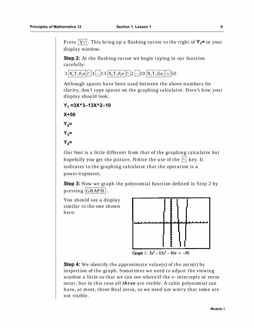
Step 3: Now we graph the polynomial function defined in Step 2 bypressing .
You should see a display similar to the one shownhere:
Step 4: We identify the approximate value(s) of the zero(s) byinspection of the graph. Sometimes we need to adjust the viewingwindow a little so that we can see where/if the x- intercepts or zerosoccur, but in this case all three are visible. A cubic polynomial canhave, at most, three Real zeros, so we need not worry that some arenot visible.
GRAPH
^
3 X,T, , ^ 3 13 X,T, , ^ 2 10 X,T, , 50n n nθ θ θ− − +
Y=
Principles of Mathematics 12 Section 1, Lesson 1 9
Module 1
a) The least zero is in the interval {−3,−1} (i.e., between −3 and −1). Aguess might be −2.0.
b) The middle zero is in the interval {2,3} (between 2 and 3). A guessmight be 2.5.
c) The greatest zero is in the interval {4,5} (between 4 and 5). Aguess might be 4.5.
Step 5: Now we will solve for the actual zeros, one by one. Thecalculator needs a few details. The TI-83 will expect to receive themin this very specific order:
Function, Variable, Guess, {Lower bound, Upper bound}
At this point, different calculators use different key sequences tosolve equations. The remaining steps 6–10 are for the TI-83. If youare using a different calculator, look in the index of its user manualunder “Solving equations”.
Be sure to:
• use the key for X.
• use the minus key within the equation itself.
• use the negation key for the guess and the bounds.
Want to know the math behind the button? Calculators and computerssolve functions with some form of Isaac Newton’s method. On a graph,Newton’s method finds solutions or zeros (x-axis crossing points) like this:using your initial “guess” and the slope of the graph at the point of yourguess, it calculates where that slope (a straight line, of course) crosses thex-axis. Then it takes the crossing point as a second guess—it goes to thegraph point directly ‘above’ or ‘below’ where the first slope crossed the x-axis. It calculates the new slope of the equation at that point, goes to wherethat new slope crosses the x-axis, and repeats the process.
If a guess is close to a zero or solution—to a point where the graph crossesthe x-axis—you can see that the graph’s slope from that point will bealmost parallel to the graph itself; the slope’s crossing point on the x-axiswill be close to the crossing point of the graph. Only a few repeats will beneeded, before it homes in on the actual crossing point. In reality, graphingcalculators perform so many repeats of Newton’s method in the time ittakes to press one button that your first guess need not be all that close to atrue solution. Just make sure that your first guess is clearly closer to onesolution (or crossing point) than it is to any other solutions. Better yet, setthe Lower and Upper Bound so that they contain only one crossing point. Ifyour guess is sort of midway between two crossing points, you can’t controlwhich one Newton’s method will find!
(-)
X,T, ,nθ
10 Section 1, Lesson 1 Principles of Mathematics 12
Module 1
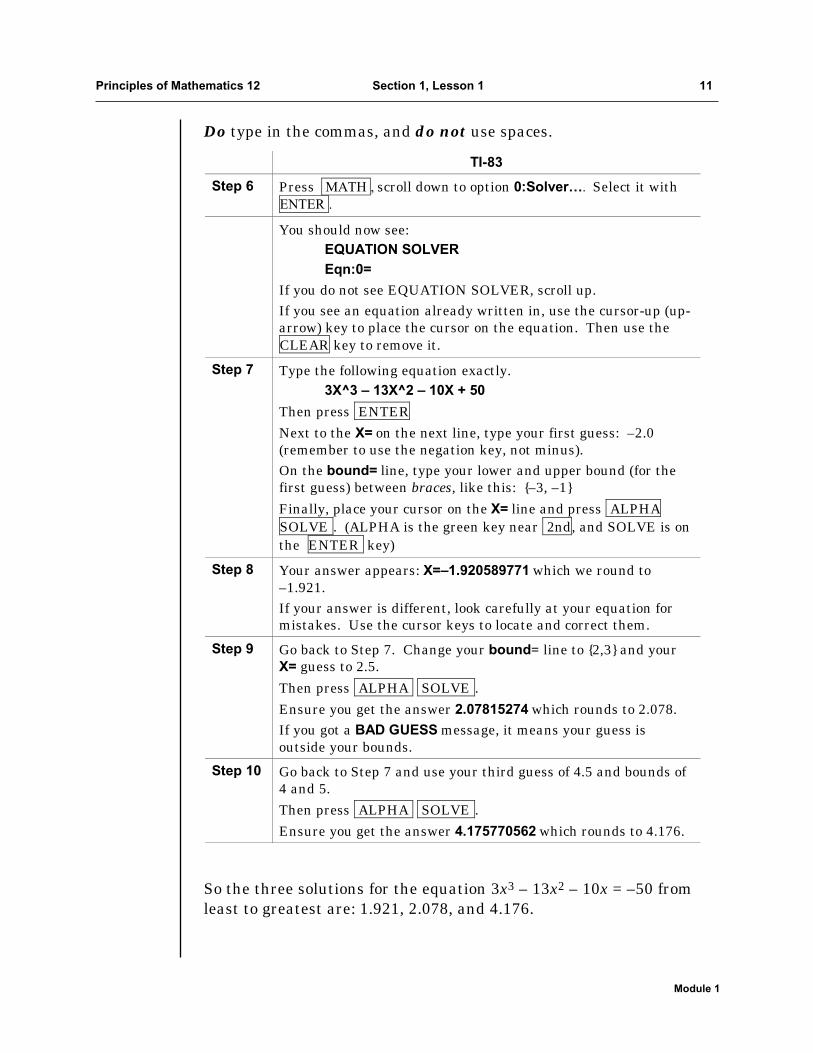
Do type in the commas, and do not use spaces.
So the three solutions for the equation 3x3 – 13x2 – 10x = –50 fromleast to greatest are: 1.921, 2.078, and 4.176.
TI-83
Step 6 Press MATH , scroll down to option 0:Solver…. Select it with ENTER .
You should now see: EQUATION SOLVER Eqn:0=
If you do not see EQUATION SOLVER, scroll up. If you see an equation already written in, use the cursor-up (up-arrow) key to place the cursor on the equation. Then use the CLEAR key to remove it.
Step 7 Type the following equation exactly. 3X^3 – 13X^2 – 10X + 50
Then press ENTER
Next to the X= on the next line, type your first guess: –2.0 (remember to use the negation key, not minus). On the bound= line, type your lower and upper bound (for the first guess) between braces, like this: {–3, –1}
Finally, place your cursor on the X= line and press ALPHA SOLVE . (ALPHA is the green key near 2nd, and SOLVE is on the ENTER key)
Step 8 Your answer appears: X=–1.920589771 which we round to –1.921. If your answer is different, look carefully at your equation for mistakes. Use the cursor keys to locate and correct them.
Step 9 Go back to Step 7. Change your bound= line to {2,3} and your X= guess to 2.5.
Then press ALPHA SOLVE .
Ensure you get the answer 2.07815274 which rounds to 2.078. If you got a BAD GUESS message, it means your guess is outside your bounds.
Step 10 Go back to Step 7 and use your third guess of 4.5 and bounds of 4 and 5. Then press ALPHA SOLVE .
Ensure you get the answer 4.175770562 which rounds to 4.176.
Principles of Mathematics 12 Section 1, Lesson 1 11
Module 1
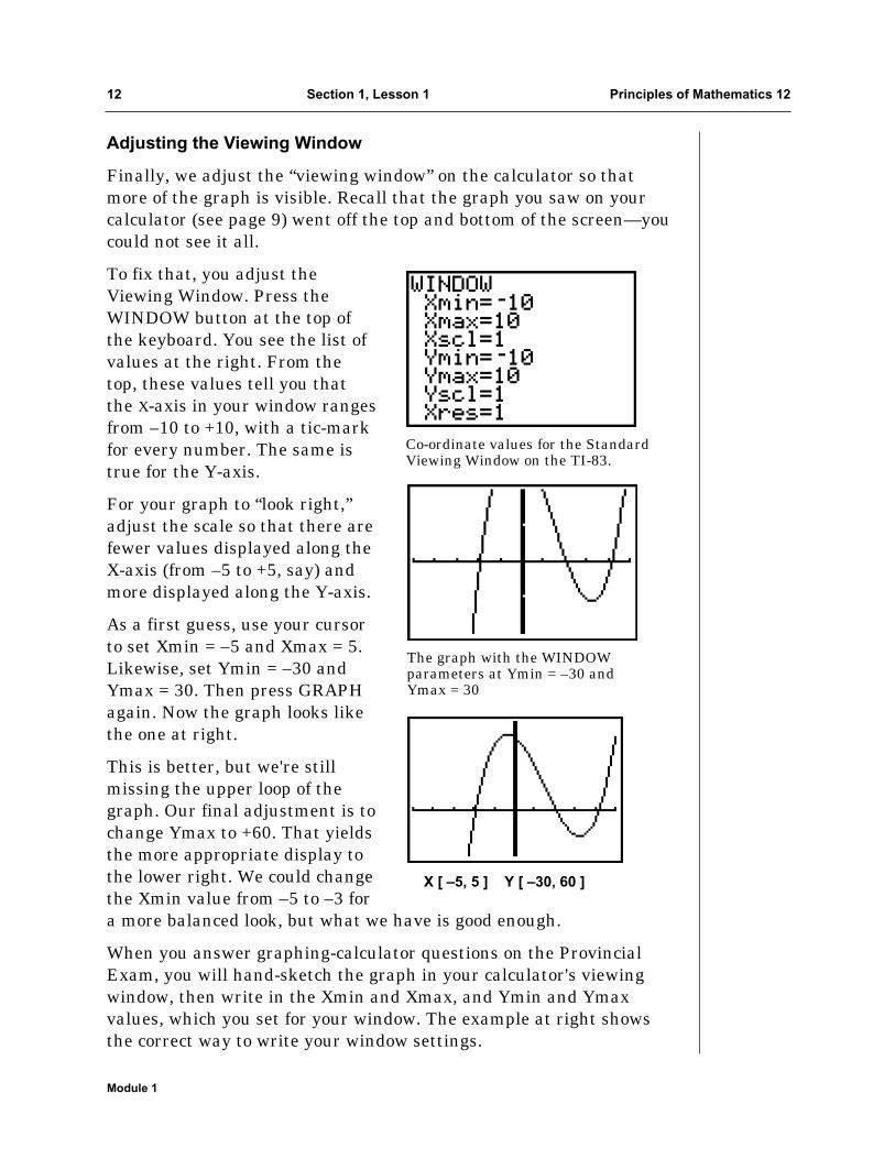
Adjusting the Viewing Window
Finally, we adjust the “viewing window” on the calculator so thatmore of the graph is visible. Recall that the graph you saw on yourcalculator (see page 9) went off the top and bottom of the screen—youcould not see it all.
To fix that, you adjust theViewing Window. Press theWINDOW button at the top ofthe keyboard. You see the list ofvalues at the right. From thetop, these values tell you thatthe X-axis in your window rangesfrom –10 to +10, with a tic-markfor every number. The same istrue for the Y-axis.
For your graph to “look right,”adjust the scale so that there arefewer values displayed along theX-axis (from –5 to +5, say) andmore displayed along the Y-axis.
As a first guess, use your cursorto set Xmin = –5 and Xmax = 5.Likewise, set Ymin = –30 andYmax = 30. Then press GRAPHagain. Now the graph looks likethe one at right.
This is better, but we're stillmissing the upper loop of thegraph. Our final adjustment is tochange Ymax to +60. That yieldsthe more appropriate display tothe lower right. We could changethe Xmin value from –5 to –3 fora more balanced look, but what we have is good enough.
When you answer graphing-calculator questions on the ProvincialExam, you will hand-sketch the graph in your calculator's viewingwindow, then write in the Xmin and Xmax, and Ymin and Ymaxvalues, which you set for your window. The example at right showsthe correct way to write your window settings.
12 Section 1, Lesson 1 Principles of Mathematics 12
Module 1
Co-ordinate values for the StandardViewing Window on the TI-83.
The graph with the WINDOWparameters at Ymin = –30 andYmax = 30
X [ –5, 5 ] Y [ –30, 60 ]
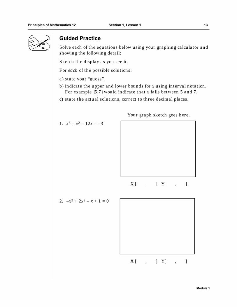
Guided Practice
Solve each of the equations below using your graphing calculator andshowing the following detail:
Sketch the display as you see it.
For each of the possible solutions:
a) state your “guess”.
b) indicate the upper and lower bounds for x using interval notation.For example {5,7} would indicate that x falls between 5 and 7.
c) state the actual solutions, correct to three decimal places.
Your graph sketch goes here.
1. x3 – x2 – 12x = –3
X [ , ] Y[ , ]
2. –x3 + 2x2 – x + 1 = 0
X [ , ] Y[ , ]
Principles of Mathematics 12 Section 1, Lesson 1 13
Module 1
3. x3 + 6x2 + 3x – 5 = 0
X [ , ] Y[ , ]
4. x3 – 3x2 = 9x – 9
X [ , ] Y[ , ]
5. 0.25x3 – 0.5x2 – 6x – 2 = 0
X [ , ] Y[ , ]
Check your answers in the Module 1 Answer Key.
14 Section 1, Lesson 1 Principles of Mathematics 12
Module 1
Lesson 2
Functions and Interval Notation
Outcomes
Upon completing this lesson, you will be able to:
• identify the domain and range of various functions using setnotation and interval notation
• find the x- and y-intercepts of any function
• perform operations on functions
Overview
The concepts of domain and range are necessary to describefunctions. Interval notation is a most convenient way to describedomain and range. We will also review combinations of functions andcomposition of functions.
Definitions
A function is a relation where each x-value has only one y-value
For any function, y = f(x), the domain is the set of possiblex-values, and the range is the set of possible y-values.
We can evaluate a function at a particular point by substitutingeither numbers or algebraic constants into the f(x) expression andsimplifying the result.
Example 1
If f(x) = x3 – 2x, find f(0), f(–2), and f(a)
f(0) = 03 – 2(0) = 0
f(–2) = (–2)3 – 2(–2) = –8 + 4 = –4
f(a) = a3 – 2a
Principles of Mathematics 12 Section 1, Lesson 2 15
Module 1
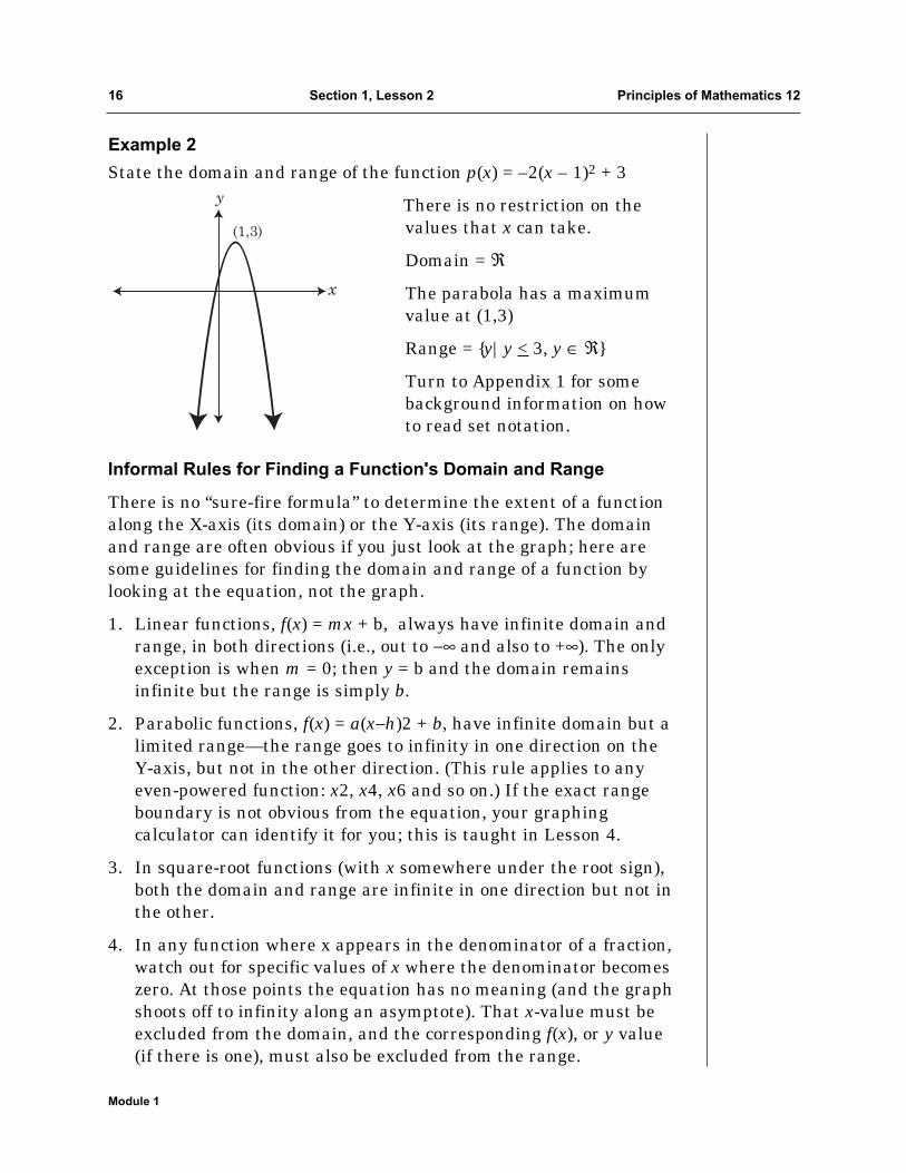
Example 2
State the domain and range of the function p(x) = –2(x – 1)2 + 3
There is no restriction on thevalues that x can take.
Domain = ℜ
The parabola has a maximumvalue at (1,3)
Range = {y|y < 3, y ∈ ℜ}
Turn to Appendix 1 for somebackground information on howto read set notation.
Informal Rules for Finding a Function's Domain and Range
There is no “sure-fire formula” to determine the extent of a functionalong the X-axis (its domain) or the Y-axis (its range). The domainand range are often obvious if you just look at the graph; here aresome guidelines for finding the domain and range of a function bylooking at the equation, not the graph.
1. Linear functions, f(x) = mx + b, always have infinite domain andrange, in both directions (i.e., out to −∞ and also to +∞). The onlyexception is when m = 0; then y = b and the domain remainsinfinite but the range is simply b.
2. Parabolic functions, f(x) = a(x−h)2 + b, have infinite domain but alimited range—the range goes to infinity in one direction on theY-axis, but not in the other direction. (This rule applies to anyeven-powered function: x2, x4, x6 and so on.) If the exact rangeboundary is not obvious from the equation, your graphingcalculator can identify it for you; this is taught in Lesson 4.
3. In square-root functions (with x somewhere under the root sign),both the domain and range are infinite in one direction but not inthe other.
4. In any function where x appears in the denominator of a fraction,watch out for specific values of x where the denominator becomeszero. At those points the equation has no meaning (and the graphshoots off to infinity along an asymptote). That x-value must beexcluded from the domain, and the corresponding f(x), or y value(if there is one), must also be excluded from the range.
(1,3)
y
x
16 Section 1, Lesson 2 Principles of Mathematics 12
Module 1
You may find these guidelines helpful as you begin Math 12 andwork through the course. Most students find that domains andranges become obvious enough that they don't need these guidelinesfor very long.
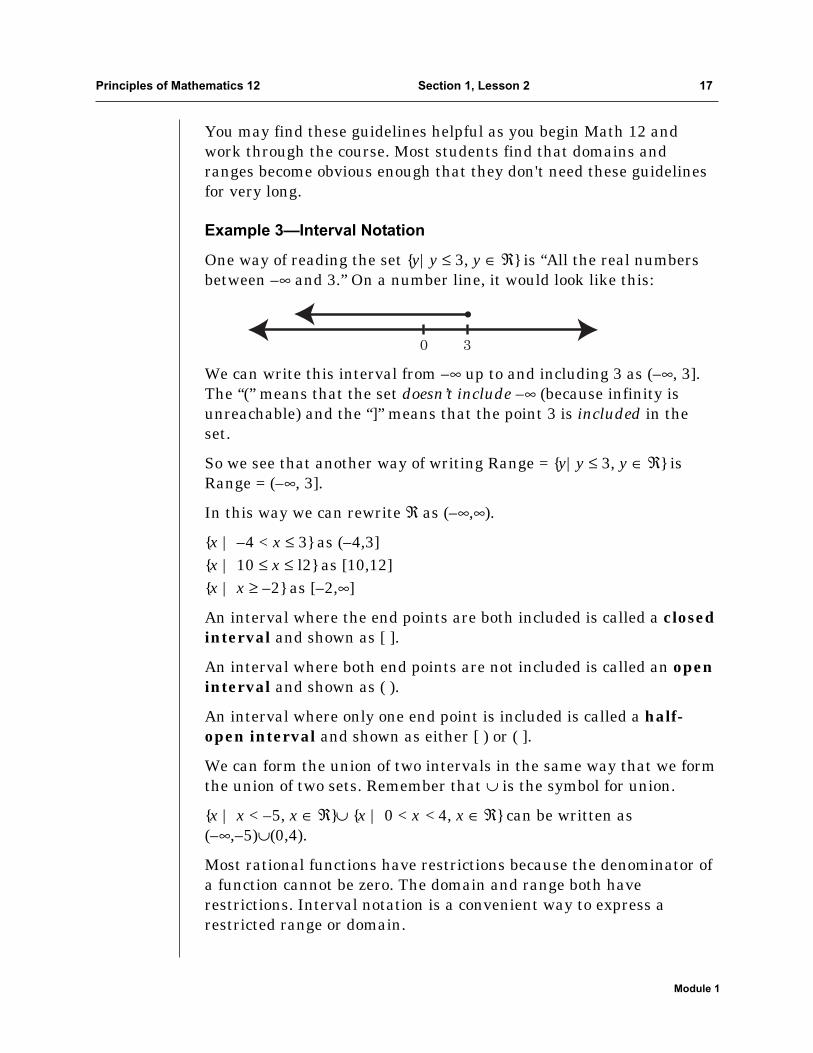
Example 3—Interval Notation
One way of reading the set {y|y ≤ 3, y ∈ ℜ} is “All the real numbersbetween –∞ and 3.” On a number line, it would look like this:
We can write this interval from –∞ up to and including 3 as (–∞, 3].The “(” means that the set doesn’t include –∞ (because infinity isunreachable) and the “]” means that the point 3 is included in theset.
So we see that another way of writing Range = {y|y ≤ 3, y ∈ ℜ} isRange = (–∞, 3].
In this way we can rewrite ℜ as (–∞,∞).
{x | –4 < x ≤ 3} as (–4,3]{x | 10 ≤ x ≤ l2} as [10,12]{x | x ≥ –2} as [–2,∞]
An interval where the end points are both included is called a closedinterval and shown as [ ].
An interval where both end points are not included is called an openinterval and shown as ( ).
An interval where only one end point is included is called a half-open interval and shown as either [ ) or ( ].
We can form the union of two intervals in the same way that we formthe union of two sets. Remember that ∪ is the symbol for union.
{x | x < –5, x ∈ ℜ}∪ {x | 0 < x < 4, x ∈ ℜ} can be written as(–∞,–5)∪(0,4).
Most rational functions have restrictions because the denominator ofa function cannot be zero. The domain and range both haverestrictions. Interval notation is a convenient way to express arestricted range or domain.
0 3
•
Principles of Mathematics 12 Section 1, Lesson 2 17
Module 1
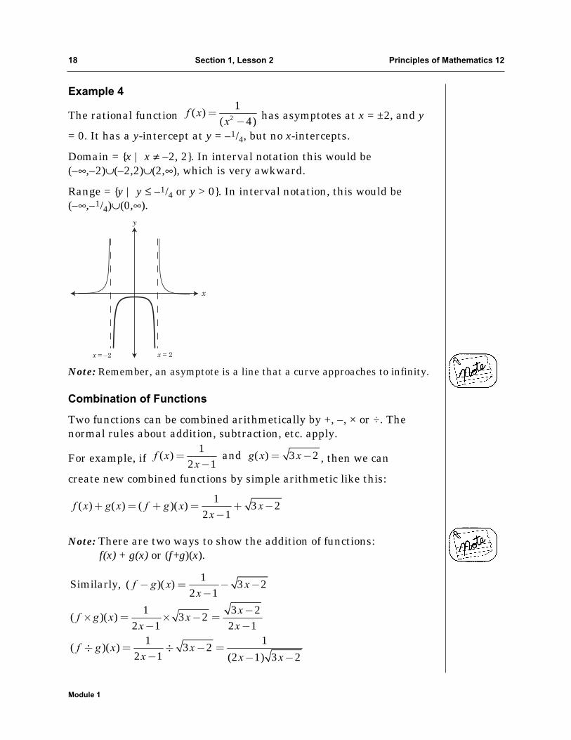
Example 4
The rational function has asymptotes at x = ±2, and y
= 0. It has a y-intercept at y = –1/4, but no x-intercepts.
Domain = {x | x ≠ –2, 2}. In interval notation this would be(–∞,–2)∪(–2,2)∪(2,∞), which is very awkward.
Range = {y | y ≤ –1/4 or y > 0}. In interval notation, this would be(–∞,–1/4)∪(0,∞).
Note: Remember, an asymptote is a line that a curve approaches to infinity.
Combination of Functions
Two functions can be combined arithmetically by +, –, × or ÷. Thenormal rules about addition, subtraction, etc. apply.
For example, if , then we can
create new combined functions by simple arithmetic like this:
Note: There are two ways to show the addition of functions: f(x) + g(x) or (f+g)(x).
1Similarly, ( )( ) 3 2
2 1
1 3 2( )( ) 3 2
2 1 2 11 1
( )( ) 3 22 1 (2 1) 3 2
f g x xx
xf g x x
x x
f g x xx x x
− = − −−
−× = × − =− −
÷ = ÷ − =− − −
1( ) ( ) ( )( ) 3 2
2 1f x g x f g x x
x+ = + = + −
−
1( ) and ( ) 3 2
2 1f x g x x
x= = −
−
x = 2x = –2
x
y
2
1( )
( 4)f x
x=
−
18 Section 1, Lesson 2 Principles of Mathematics 12
Module 1
Rule: When functions are combined arithmetically like that, thedomain of the result is the intersection of domains from the twofunctions—it’s the set of all points that belong in both the originaldomains. The same is true of the combined range—it’s theintersection of the two separate ranges.
That intersection-of-domains rule applies for all four arithmeticoperations, between any two functions. But the division operation (f÷g)has an additional rule: the combined domain and range cannot includeany value that makes the new denominator go to zero.
Note: Whenever this course uses a plain square root sign, it refers onlyto the positive square root. This definition is common in most modern mathematics.
Examples: If you solve , then the answer is x = 2 but not
x = –2. If it wants the negative root, this course will ask you to
solve . If this course asks you for both roots, it will ask you to
solve .
Example 5
Using the above two functions f and g, find the domain and range off+g, f–g, f×g, and f÷g.
Solution
By inspection, domain of f = {x|x ≠ } and the range of
f = {y | y ≠ 0}. x = and y = 0 are not allowed because f cannot
have a zero in the denominator.
Similarly, domain of g = [ ,∞)
Range of g = [0,∞)
Now for the intersections. Remember that ∩ is the symbol forintersection:
Domain of (f+g) = domain of (f–g) = domain of (f×g) = {x | x ≠ } ∩ [ ,∞) = [ ,∞).2
323
12
23
12
12
4x = ±
4x = −
4x =
Principles of Mathematics 12 Section 1, Lesson 2 19
Module 1
The square root of a negativenumber is not real so g cannot
be less than . But the value
is in the domain of g.23
23
20 Section 1, Lesson 2 Principles of Mathematics 12
Module 1
Range of (f+g) = range of (f–g) = range of (f×g) = [y | y ≠ 0} ∪ [0,∞) =[0,∞).
The domain of (f÷g) = ( ,∞) instead of [ ,∞). That’s because g(x) is inthe denominator and g( ) = 0. So must be deleted from thecombined domain.
The range of (f÷g) is (0,∞), just as it is for f+g, f–g, and (f×g). Thevalue 0 was excluded from the range of f already, so it’s not going toappear in the range of the combined function.
Sometimes, when you write the range or domain of a combinedfunction, it may be simpler to leave the intersection symbol ∩ in youranswer.
Finding Intercepts
For more complex functions, we often need to know the x- and y-intercepts in order to find the domain and range.
Rule: To find the y-intercept, set x = 0. To find the x-intercept, set y = 0.
Example 6
Find the x- and y-intercepts for the function, f(x) = x2(x + 1)(x – 2)
Solution
y-intercept: Set x = 0
f(0) = 02(0 + 1)(0 – 2) = 0
x-intercepts: Set y = 0
Solve: x2(x + 1)(x – 2) = 0
x2 = 0, or x + 1 = 0, or x – 2 = 0
∴x = 0, –1, or 2
Composition of Functions
A composition of two functions is when they are arranged so that oneis a function of the other.
Composition is not the same as “combination” using arithmeticoperations between functions!
23
23
23
23
The composition is written as (f°g)(x) = f(g(x)) or as (g°f)(x) = g(f(x)),either with a small hollow circle for the operation, or with onefunction nested inside the other. In this course, f(g(x)) is the usualnotation but we’ll start by using both forms.
Example 7
If f(x) = x – 3 and g(x) = 2x + 1, find (f°g)(x) and (g°f)(x).
(f°g)(x) = f(g(x))
= f(2x + 1) Substitute formula for g(x)
= (2x + 1) – 3 Apply formula for f(x)
= 2x – 2 Simplify
(g°f)(x) = g(f(x))= g(x – 3) Substitute formula for f(x)
= 2(x – 3) + 1 Apply formula for g(x)
= 2x – 5 Simplify
Notes to remember:
1. As Example 7 suggests, (g°f)(x) ≠ (f°g)(x) except in special cases.
2. For (f°g)(x) = f(g(x)), the range of g becomes the domain of f.
Example 8
If f(x) = and h(x) = 2(x + 1), write an equation for (f°h)(x).
Specify the domain and range.
Solution
(f°h)(x) = f(h(x))
To find the restrictions on the domain, remember that thedenominator cannot be zero.
( )2 1 0
1
x
x
+ ≠
≠ −
( )3
2 1x=
+
3x
Principles of Mathematics 12 Section 1, Lesson 2 21
Module 1
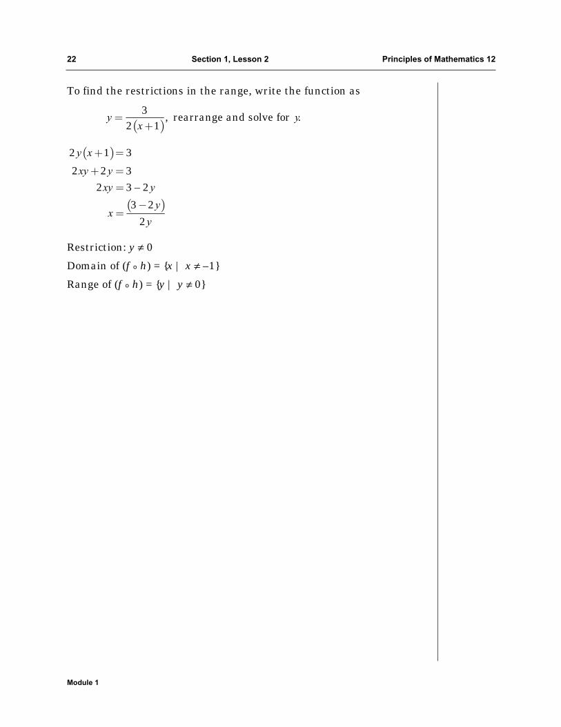
To find the restrictions in the range, write the function as
Restriction: y ≠ 0
Domain of (f ° h) = {x | x ≠ –1}
Range of (f ° h) = {y | y ≠ 0}
( )
( )
2 1 3
2 2 32 3 – 2
3 2
2
y x
xy y
xy y
yx
y
+ =
+ ==
−=
( )3
, rearrange and solve for .2 1
y yx
=+
22 Section 1, Lesson 2 Principles of Mathematics 12
Module 1
Guided Practice
1. Given that f(x) = 4x2 – x + 3 and g(x) = 1 – 2x, find:
a) f(0) g) (f+g)(x)
b) g(0) h) (g – f)(x)
c) f(–2) i) (f×g)(–2)
d) g(1/4) j) (f÷g)(0)
e) f(a) k) (g÷f)(b – 1)
f) g(b – 1)
2. Determine the x- and y-intercepts for the following functions:
a) f(x) = 2x2 – 8
b)
c) k(x) = 5 – x
3. Using the information from your answers to question 2, write thedomain and range for each function using:
i) set notation
ii) interval notation
4. Given that and q(x) = 3x + l:
a) determine each of the following:
i) p(q(x))
ii) p(q(3))
iii) q(p(a))
b) find the domain and range of:
i) p(q(x))
ii) q(p(x))
Check your answers in the Module 1 Answer Key.
( ) 4p x x= −
( ) 2 5g x x= +
Principles of Mathematics 12 Section 1, Lesson 2 23
Module 1
Lesson 3
Inverse Functions
Outcomes
Upon completing this lesson, you will be able to:
• verify that two functions are inverses of each other
• identify one-to-one functions
• find inverse functions
Overview
Many of the important new functions you will learn about inPrinciples of Mathematics 12 are the inverses of other functions.The concept of an inverse is essential to solving mathematicsproblems.
Definition
Inverse Function: Let f and g be two functions such that f(g(x)) = x for every x in the domain of g and g(f(x)) = x for every xin the domain of f.
Then the function g is the inverse of the function f, denoted by f–1.Thus f(f–1(x)) = x and f–1(f(x)) = x. The domain of f must be equalto the range of f–1 and vice versa.
The graphs of f and f–1 are related to each other in this way. Ifthe point (a, b) lies on the graph f, then the point (b, a) lieson the graph of f–1 and vice versa. This means that the graphof f is a reflection of the graph of f–1 in the line y = x.
24 Section 1, Lesson 3 Principles of Mathematics 12
Module 1
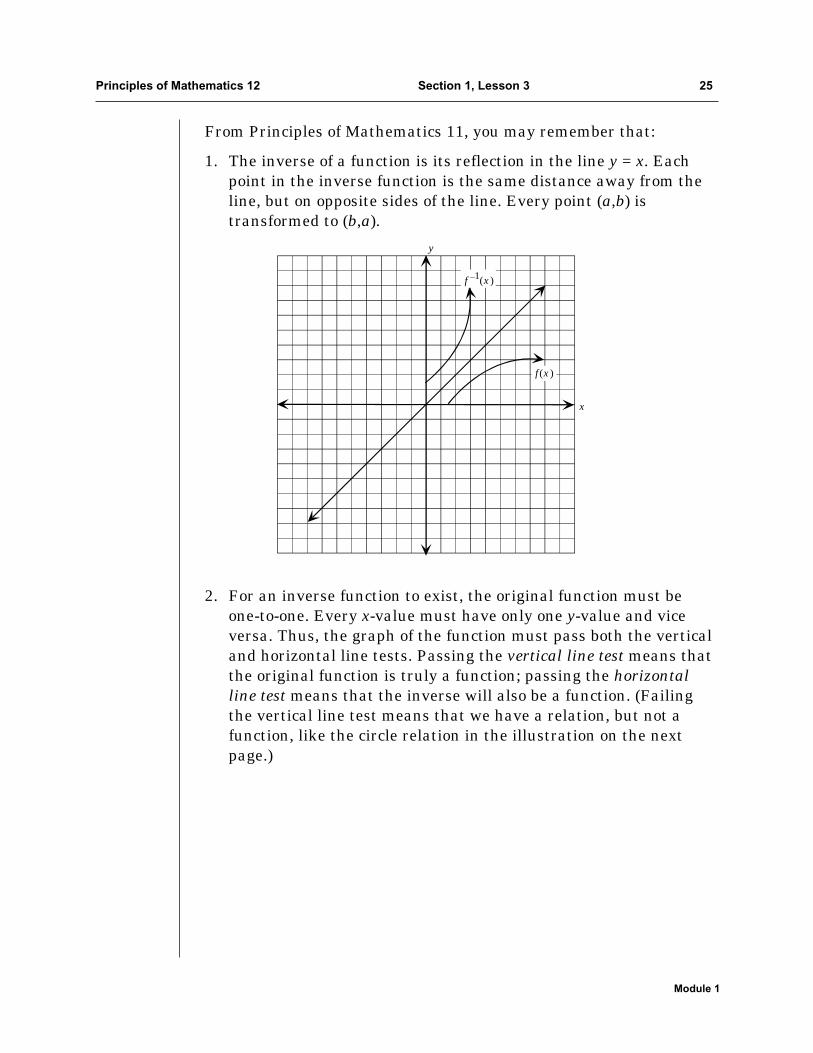
From Principles of Mathematics 11, you may remember that:
1. The inverse of a function is its reflection in the line y = x. Eachpoint in the inverse function is the same distance away from theline, but on opposite sides of the line. Every point (a,b) istransformed to (b,a).
2. For an inverse function to exist, the original function must beone-to-one. Every x-value must have only one y-value and viceversa. Thus, the graph of the function must pass both the verticaland horizontal line tests. Passing the vertical line test means thatthe original function is truly a function; passing the horizontalline test means that the inverse will also be a function. (Failingthe vertical line test means that we have a relation, but not afunction, like the circle relation in the illustration on the nextpage.)
x
y
f(x )
f (x )1
Principles of Mathematics 12 Section 1, Lesson 3 25
Module 1
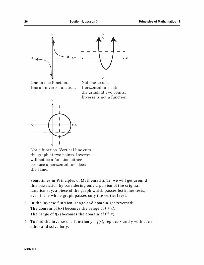
Sometimes in Principles of Mathematics 12, we will get aroundthis restriction by considering only a portion of the originalfunction say, a piece of the graph which passes both line tests,even if the whole graph passes only the vertical test.
3. In the inverse function, range and domain get reversed:The domain of f(x) becomes the range of f–1(x).The range of f(x) becomes the domain of f–1(x).
4. To find the inverse of a function y = f(x), replace x and y with eachother and solve for y.
One-to-one function.
Has an inverse function.
Not one-to-one.
Horizontal line cuts
the graph at two points.
Inverse is not a function.
Not a function. Vertical line cuts
the graph at two points. Inverse
will not be a function either
because a horizontal line does
the same.
y y
y
x
xx
26 Section 1, Lesson 3 Principles of Mathematics 12
Module 1
Principles of Mathematics 12 Section 1, Lesson 3 27
Module 1
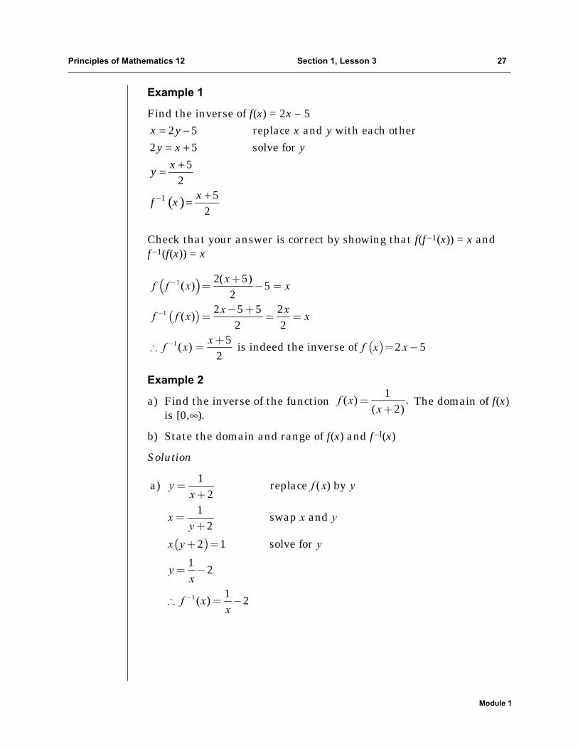
Example 1
Find the inverse of f(x) = 2x – 5
Check that your answer is correct by showing that f(f–1(x)) = x andf–1(f(x)) = x
Example 2
a) Find the inverse of the function The domain of f(x)is [0,∞).
b) State the domain and range of f(x) and f–l(x)
Solution
( )
1
1a) replace ( ) by
21
swap and 2
2 1 solve for
12
1( ) 2
y f x yx
x x yy
x y y
yx
f xx
−
=+
=+
+ =
= −
∴ = −
1( ) .
( 2)f x
x=
+
( )
( )
( )
1
1
1
2( 5)( ) 5
22 5 5 2
( )2 2
5( ) is indeed the inverse of 2 5
2
xf f x x
x xf f x x
xf x f x x
−
−
−
+= − =
− += = =
+∴ = = −
( )1
2 5 replace and with each other2 5 solve for
52
52
x y x yy x y
xy
xf x−
= −= +
+=
+=
b) domain of f = [0,∞) (given)
range of f = (0, ] (the maximum value of f is when x = 0)
domain of f–1 = range of f = (0, ]
range of f–1 = domain of f = [0,∞)
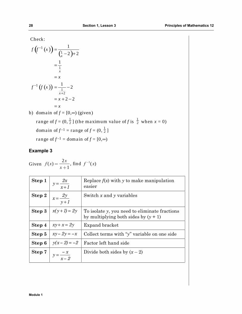
Example 3
Given
Step 11
2
+=
x
xy
Replace f(x) with y to make manipulation easier
Step 21
2
+=
y
yx
Switch x and y variables
Step 3 yyx 2)1( =+ To isolate y, you need to eliminate fractions by multiplying both sides by (y + 1)
Step 4 yxxy 2=+ Expand bracket
Step 5 xyxy =2 Collect terms with “y” variable on one side
Step 6 2)2( =xy Factor left hand side
Step 72
=x
xy
Divide both sides by (x – 2)
12( ) , find ( )
1x
f x f xx
−=+
12
12
12
( )( ) ( )
( )( )
11
1
11
2
Check:12 2
1
12
2 2
x
x
x
f f x
x
f f x
xx
−
−
+
=− +
=
=
= −
= + −=
28 Section 1, Lesson 3 Principles of Mathematics 12
Module 1
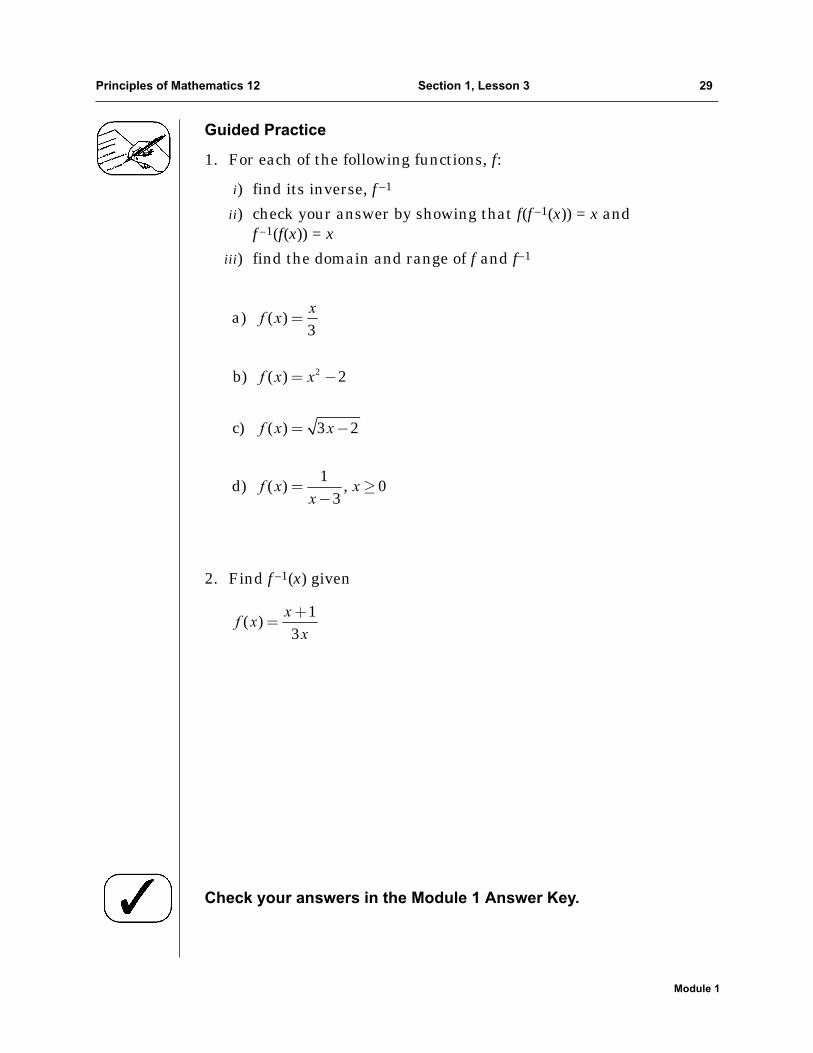
Guided Practice
1. For each of the following functions, f:
i) find its inverse, f–1
ii) check your answer by showing that f(f–1(x)) = x and f–1(f(x)) = x
iii) find the domain and range of f and f–1
2. Find f–1(x) given
Check your answers in the Module 1 Answer Key.
1( )
3x
f xx
+=
2
a) ( )3
b) ( ) 2
c) ( ) 3 2
1d) ( ) , 0
3
xf x
f x x
f x x
f x xx
=
= −
= −
= ≥−
Principles of Mathematics 12 Section 1, Lesson 3 29
Module 1

Notes
30 Section 1, Lesson 3 Principles of Mathematics 12
Module 1
Module 1
Principles of Mathematics 12 Section 1, Lesson 4 31
Lesson 4
Polynomial Functions and Their Graphs
Outcomes
Upon completing this lesson, you will be able to:
• identify a polynomial function
• relate its factors to its zeroes
• graph a polynomial function
Overview
A polynomial function is an expression that can be written in
negative integer. In the above polynomial, each of the anx parts iscalled a term. Terms are always added together (or subtracted) inpolynomials—never multiplied. The ai values are called coefficientsof the terms.
Notes
1. The graph of a polynomial function is continuous. This means thegraph has no breaks—you could sketch the graph without liftingyour pencil from the paper.
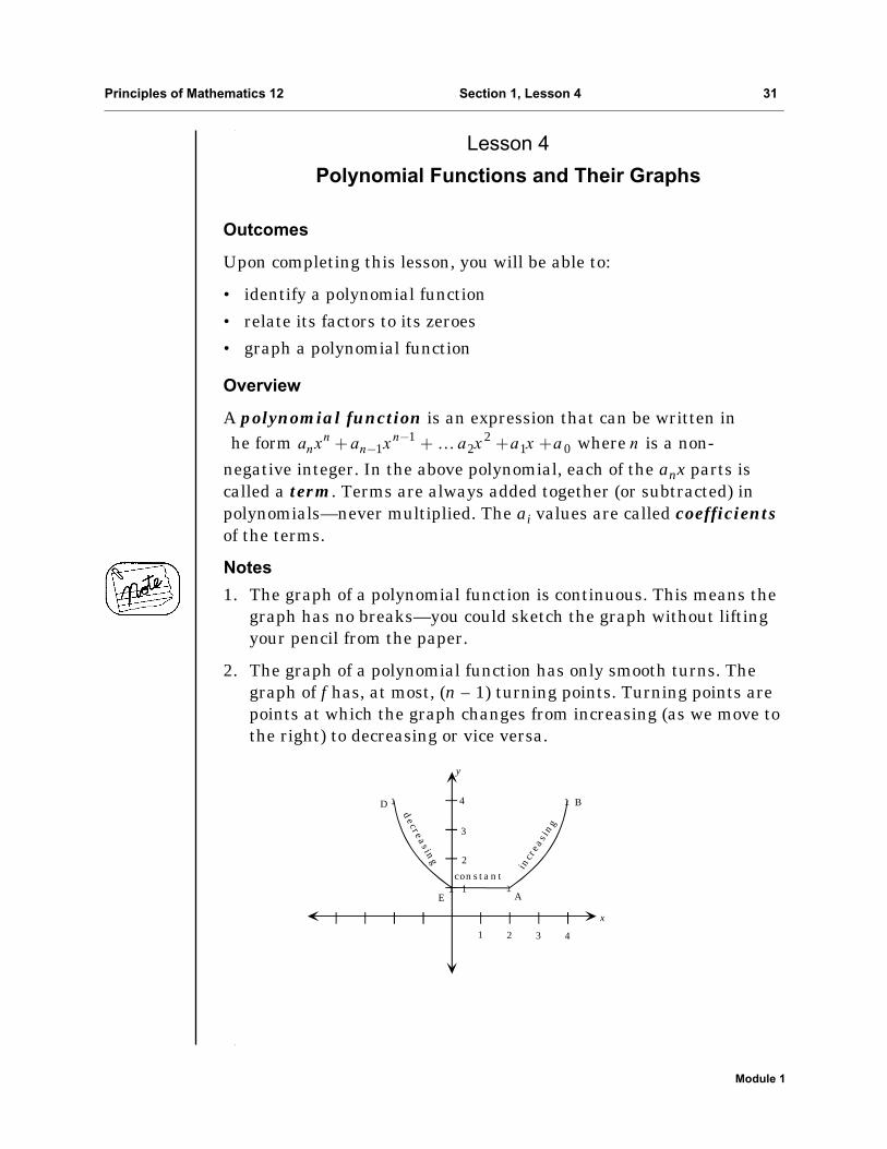
2. The graph of a polynomial function has only smooth turns. Thegraph of f has, at most, (n – 1) turning points. Turning points arepoints at which the graph changes from increasing (as we move tothe right) to decreasing or vice versa.
1 2 3 4
4
3
2
1
l
l l
l
x
y
B
AE
D
decreasing
constant
incr
easi
ng
1 21 2 1 0he form where is a non-…n n
n na x a x a x a x a n−−+ + + +
32 Section 1, Lesson 4 Principles of Mathematics 12
Module 1
The function shown above is decreasing in the interval from D toE, it remains constant from E to A, and it is increasing in theinterval from A to B. (Incidentally, because of its sharp cornersand its flat section, it cannot be the graph of a polynomialfunction.)
For the graphs that you investigated, the cubic equation will haveat most (3 – 1) turns, or two turns. For the graphs that youinvestigated, the quartic equations will have at most (4 – 1) turns, or 3 turns.
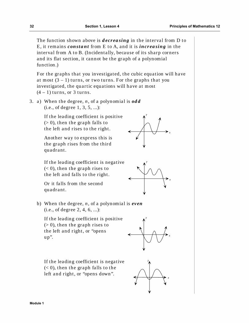
3. a) When the degree, n, of a polynomial is odd(i.e., of degree 1, 3, 5, ...):
If the leading coefficient is positive(> 0), then the graph falls tothe left and rises to the right.
Another way to express this isthe graph rises from the thirdquadrant.
If the leading coefficient is negative(< 0), then the graph rises tothe left and falls to the right.
Or it falls from the secondquadrant.
b) When the degree, n, of a polynomial is even(i.e., of degree 2, 4, 6, ...):
If the leading coefficient is positive(> 0), then the graph rises tothe left and right, or “opensup”.
If the leading coefficient is negative(< 0), then the graph falls to theleft and right, or “opens down”.
x
y
x
y
x
y
x
y
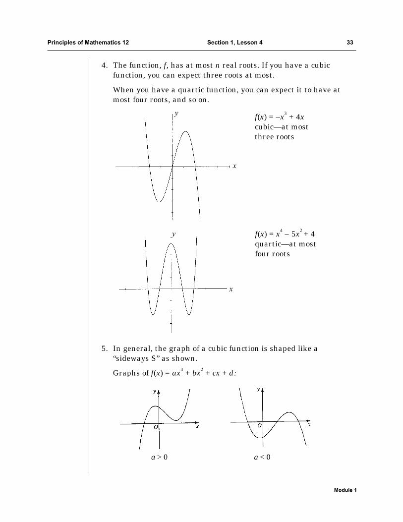
4. The function, f, has at most n real roots. If you have a cubicfunction, you can expect three roots at most.
When you have a quartic function, you can expect it to have atmost four roots, and so on.
5. In general, the graph of a cubic function is shaped like a“sideways S” as shown.
Graphs of f(x) = ax3 + bx2 + cx + d:
a > 0 a < 0
f(x) = x4 – 5x2 + 4quartic—at mostfour roots
f(x) = –x3 + 4xcubic—at mostthree roots
Principles of Mathematics 12 Section 1, Lesson 4 33
Module 1
x
y
x
y
In general, the graph of a quartic equation has a “W shape” or an“M shape.”
Graphs of f(x) = ax4 + bx3 + cx2 + dx + e:
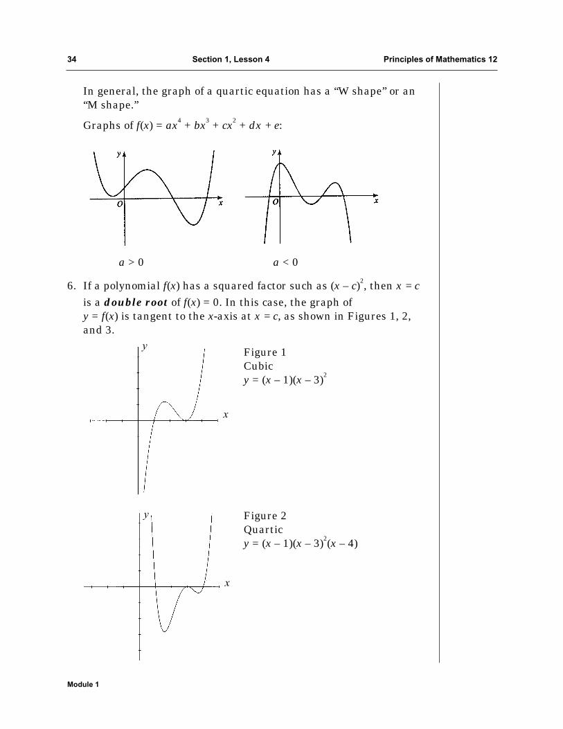
6. If a polynomial f(x) has a squared factor such as (x – c)2, then x = cis a double root of f(x) = 0. In this case, the graph of y = f(x) is tangent to the x-axis at x = c, as shown in Figures 1, 2,and 3.
Figure 2Quarticy = (x – 1)(x – 3)2(x – 4)
Figure 1Cubicy = (x – 1)(x – 3)2
a > 0 a < 0
34 Section 1, Lesson 4 Principles of Mathematics 12
Module 1
y
x
y
x
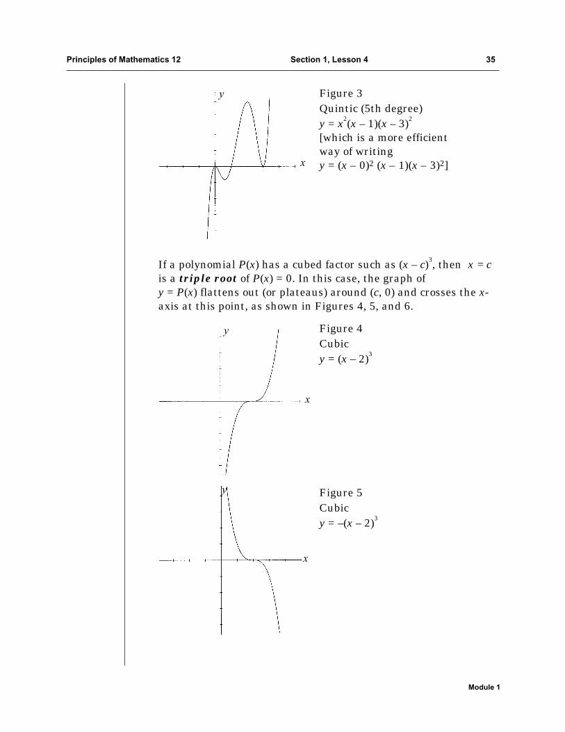
If a polynomial P(x) has a cubed factor such as (x – c)3, then x = cis a triple root of P(x) = 0. In this case, the graph of y = P(x) flattens out (or plateaus) around (c, 0) and crosses the x-axis at this point, as shown in Figures 4, 5, and 6.
Figure 5Cubicy = –(x – 2)3
Figure 4Cubicy = (x – 2)3
Figure 3Quintic (5th degree)y = x2(x – 1)(x – 3)2
[which is a more efficientway of writing y = (x – 0)2 (x – 1)(x – 3)2]
Principles of Mathematics 12 Section 1, Lesson 4 35
Module 1
y
x
y
x
y
x
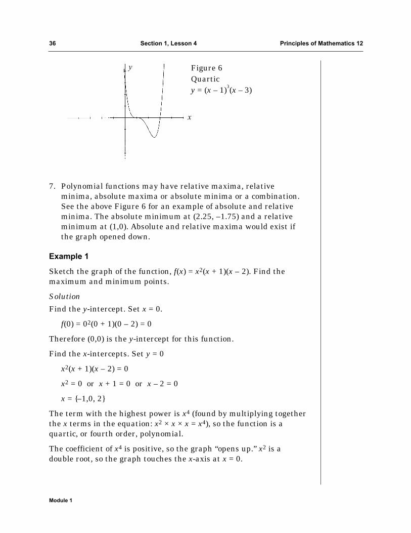
7. Polynomial functions may have relative maxima, relativeminima, absolute maxima or absolute minima or a combination.See the above Figure 6 for an example of absolute and relativeminima. The absolute minimum at (2.25, –1.75) and a relativeminimum at (1,0). Absolute and relative maxima would exist ifthe graph opened down.
Example 1
Sketch the graph of the function, f(x) = x2(x + 1)(x – 2). Find themaximum and minimum points.
Solution
Find the y-intercept. Set x = 0.
f(0) = 02(0 + 1)(0 – 2) = 0
Therefore (0,0) is the y-intercept for this function.
Find the x-intercepts. Set y = 0
x2(x + 1)(x – 2) = 0
x2 = 0 or x + 1 = 0 or x – 2 = 0
x = {–1,0, 2}
The term with the highest power is x4 (found by multiplying togetherthe x terms in the equation: x2 × x × x = x4), so the function is aquartic, or fourth order, polynomial.
The coefficient of x4 is positive, so the graph “opens up.” x2 is adouble root, so the graph touches the x-axis at x = 0.
Figure 6Quarticy = (x – 1)3(x – 3)
36 Section 1, Lesson 4 Principles of Mathematics 12
Module 1
y
x
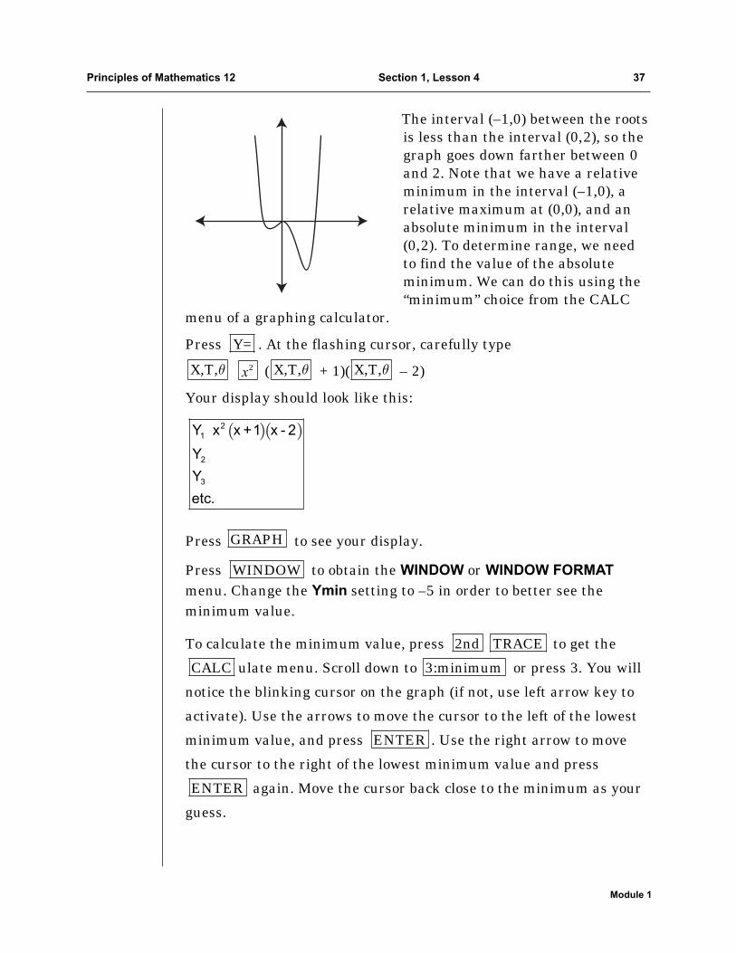
The interval (–1,0) between the rootsis less than the interval (0,2), so thegraph goes down farther between 0and 2. Note that we have a relativeminimum in the interval (–1,0), arelative maximum at (0,0), and anabsolute minimum in the interval(0,2). To determine range, we needto find the value of the absoluteminimum. We can do this using the“minimum” choice from the CALC
menu of a graphing calculator.
Press . At the flashing cursor, carefully type
( + 1)( – 2)
Your display should look like this:
Press to see your display.
Press to obtain the WINDOW or WINDOW FORMATmenu. Change the Ymin setting to –5 in order to better see theminimum value.
To calculate the minimum value, press to get the
ulate menu. Scroll down to or press 3. You will
notice the blinking cursor on the graph (if not, use left arrow key to
activate). Use the arrows to move the cursor to the left of the lowest
minimum value, and press . Use the right arrow to move
the cursor to the right of the lowest minimum value and press
again. Move the cursor back close to the minimum as your
guess.
ENTER
ENTER
3:minimumCALC
TRACE2nd
WINDOW
GRAPH
( )( )21
2
3
Y x x +1 x - 2
Y
Y
etc.
X,T,θX,T,θ2xX,T,θ
Y=
Principles of Mathematics 12 Section 1, Lesson 4 37
Module 1
Press again.
The minimum occurs at (+1.443001, –2.833422).
Therefore range = [–2.833,∞), or {y|y ≥ –2.833]. We use a closed intervalbecause the graph reaches down to approximately –2.833.
Example 2
Inspect the following polynomial functions and determine their basicshape and orientation.
Determine the domain and range of each.
a) f(x) = x3 – 4x
b) g(x) = –x6 + 4x2
c) k(x) = –x5 + 4x3 – 6
Hint: The absolute minimum or absolute maximum always definesthe range.
Solutions
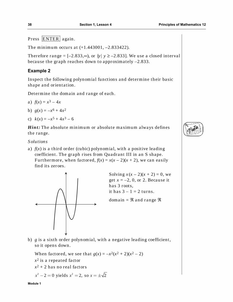
a) f(x) is a third order (cubic) polynomial, with a positive leadingcoefficient. The graph rises from Quadrant III in an S shape.Furthermore, when factored, f(x) = x(x – 2)(x + 2), we can easilyfind its zeroes.
Solving x (x – 2)(x + 2) = 0, weget x = –2, 0, or 2. Because ithas 3 roots, it has 3 – 1 = 2 turns.
domain = ℜ and range ℜ
b) g is a sixth order polynomial, with a negative leading coefficient,so it opens down.
When factored, we see that g(x) = –x2(x2 + 2)(x2 – 2)x2 is a repeated factorx2 + 2 has no real factors
2 22 0 yields 2, so 2x x x− = = =±
ENTER
38 Section 1, Lesson 4 Principles of Mathematics 12
Module 1
Principles of Mathematics 12 Section 1, Lesson 4 39
Module 1
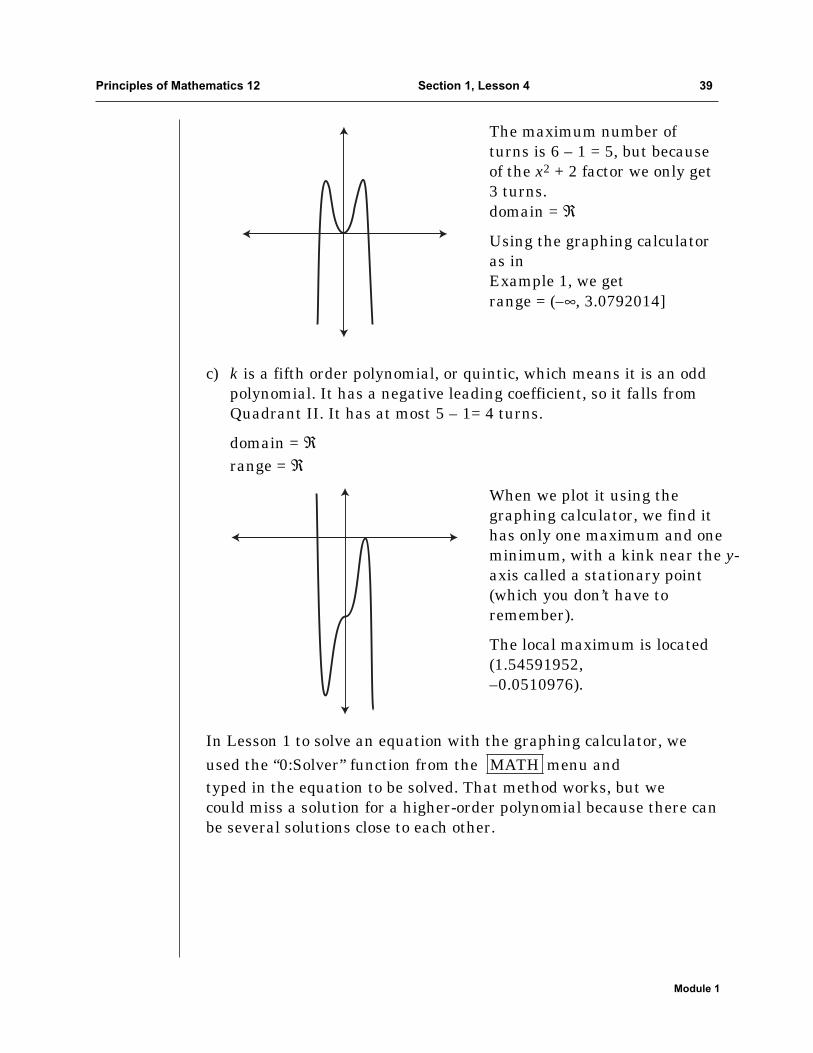
The maximum number ofturns is 6 – 1 = 5, but becauseof the x2 + 2 factor we only get3 turns.domain = ℜ
Using the graphing calculatoras in Example 1, we getrange = (–∞, 3.0792014]
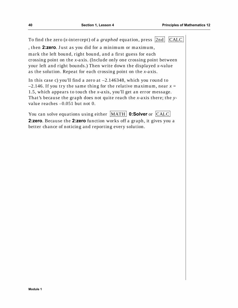
c) k is a fifth order polynomial, or quintic, which means it is an oddpolynomial. It has a negative leading coefficient, so it falls fromQuadrant II. It has at most 5 – 1= 4 turns.
domain = ℜrange = ℜ
When we plot it using thegraphing calculator, we find ithas only one maximum and oneminimum, with a kink near the y-axis called a stationary point(which you don’t have toremember).
The local maximum is located(1.54591952,–0.0510976).
In Lesson 1 to solve an equation with the graphing calculator, weused the “0:Solver” function from the menu andtyped in the equation to be solved. That method works, but wecould miss a solution for a higher-order polynomial because there canbe several solutions close to each other.
MATH
To find the zero (x-intercept) of a graphed equation, press
, then 2:zero. Just as you did for a minimum or maximum,mark the left bound, right bound, and a first guess for eachcrossing point on the x-axis. (Include only one crossing point betweenyour left and right bounds.) Then write down the displayed x-valueas the solution. Repeat for each crossing point on the x-axis.
In this case c) you'll find a zero at –2.146348, which you round to–2.146. If you try the same thing for the relative maximum, near x =1.5, which appears to touch the x-axis, you'll get an error message.That’s because the graph does not quite reach the x-axis there; the y-value reaches –0.051 but not 0.
You can solve equations using either 0:Solver or 2:zero. Because the 2:zero function works off a graph, it gives you abetter chance of noticing and reporting every solution.
CALCMATH
CALC2nd
40 Section 1, Lesson 4 Principles of Mathematics 12
Module 1
Guided Practice
1. Rewrite each polynomial in descending order. Determine:
i) the degree of the polynomial
ii) the maximum number of turns in the graph
2. State the left-right behavior of the graphs in question 1, as towhether they open up, open down, rise from Quadrant III, or fallfrom Quadrant II.
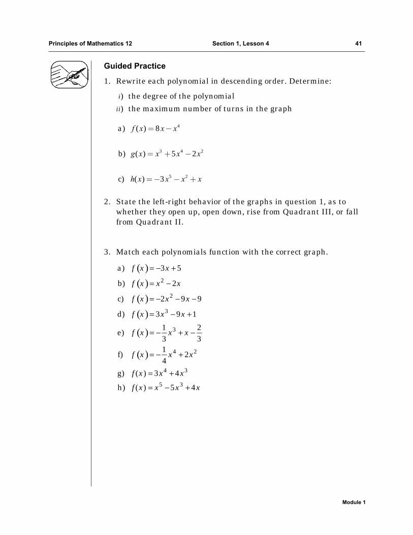
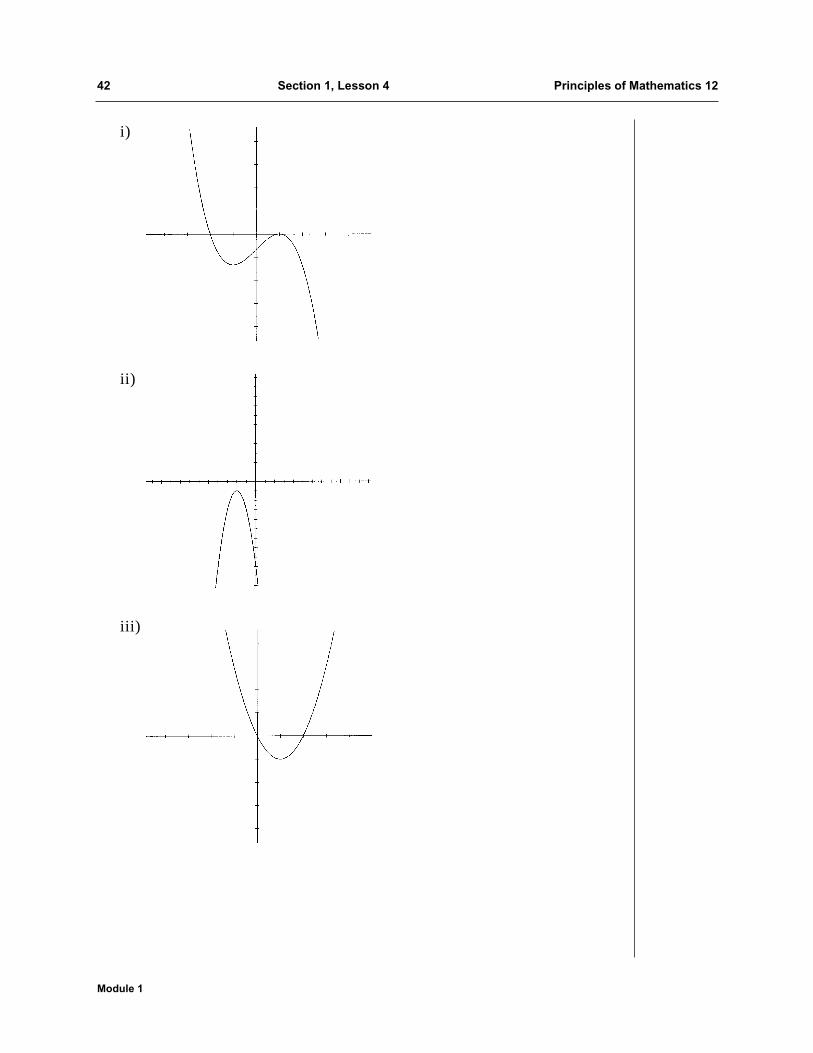
3. Match each polynomials function with the correct graph.
( )( )( )( )
( )
( )
2
2
3
3
4 2
4 3
5 3
a) 3 5
b) 2
c) 2 9 9
d) 3 9 1
1 2e)
3 31
f) 24
g) ( ) 3 4
h) ( ) 5 4
f x x
f x x x
f x x x
f x x x
f x x x
f x x x
f x x x
f x x x x
= − +
= −
= − − −
= − +
= − + −
= − +
= +
= − +
4
3 4 2
5 2
a) ( ) 8
b) ( ) 5 2
c) ( ) 3
f x x x
g x x x x
h x x x x
= −
= + −
=− − +
Principles of Mathematics 12 Section 1, Lesson 4 41
Module 1
i)
ii)
iii)
42 Section 1, Lesson 4 Principles of Mathematics 12
Module 1
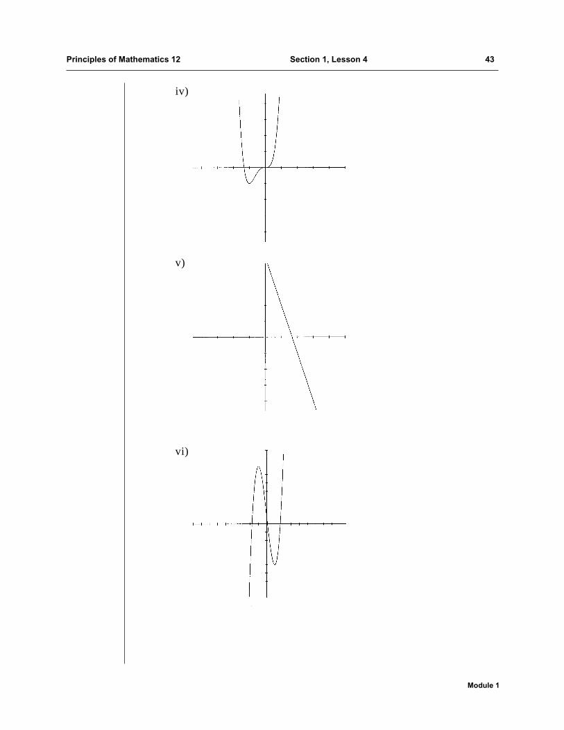
iv)
v)
vi)
Principles of Mathematics 12 Section 1, Lesson 4 43
Module 1
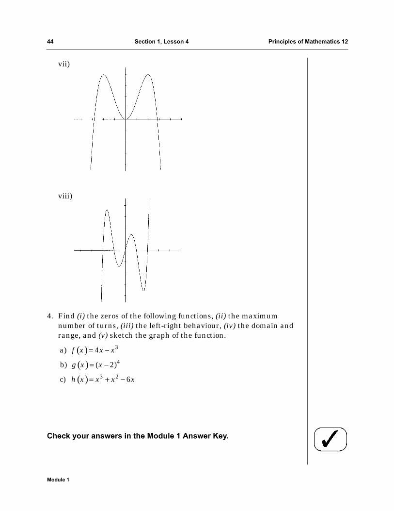
vii)
viii)
4. Find (i) the zeros of the following functions, (ii) the maximumnumber of turns, (iii) the left-right behaviour, (iv) the domain andrange, and (v) sketch the graph of the function.
Check your answers in the Module 1 Answer Key.
( )( )( )
3
4
3 2
a) 4
b) ( 2)
c) 6
f x x x
g x x
h x x x x
= −
= −
= + −
44 Section 1, Lesson 4 Principles of Mathematics 12
Module 1
Principles of Mathematics 12 Section 1, Review 45
Module 1
Review
1. Solve the following equations using your graphing calculator.
2.
3. i) Determine the x- and y-intercepts of these functions.ii) Find the domain and range.
2
2
a) ( ) 1 2
b) ( ) 2( 2) 4
c) ( ) ( 2) ( 4)( 2)
f x x
g x x
h x x x x
= −
= + −
= + − −
1
1
a) (2)b) ( 1)c) ( )(4)d) ( )(4)e) ( 4)f) ( )(1)g) ( )( )
h) ( ( ))i) ( )( 2)
j) ( )
f
g
f g
f g
f a
g f
f g x
f f x
f g t
g x
−
−
−+÷
+
× +
( ) 2If 3 3 1 and ( ) 2 1, find:f x x x g x x= + − = +
3 2
4 2
5 3 2
3 2
a) 2 4 7
b) 2 3 4
c) 4 3
d) 0.4 0.78 2.4 7 0
x x x
x x
x x x x
x x x
+ − =
+ =
− = −
− + + =
4. Find the inverse of the following functions.
5. Sketch the graphs of the following functions. Label the interceptsand give the domain and range of each.
Check your answers In the Module 1 Answer Key.
Now do the section assignment which follows this section. When it iscomplete, send it in for marking.
3 2
2
a) ( ) 2
b) ( ) 2( 9)( 2)(2 1)
f x x x
g x x x x
= + −
=− − + −
2
2
a) ( ) 5 2
b) ( ) ( 1) 3
1c) ( )
1
f x x
g x x
h xx
= −
= + −
=−
46 Section 1, Review Principles of Mathematics 12
Module 1
Student's StudentName _______________________________ No. __________________________
Address _______________________________ School __________________________
_______________________________
Student's_______________________________ FAX No. __________________________
Instructor'sName _______________________________Date Sent __________________________
PRINCIPLES OF MATHEMATICS 12
Section Assignment 1.1
Your instructor will fill in this box with your percentage mark and lettergrade on the section assignment:
Comments/Questions:
Principles of Mathematics 12 Section Assignment 1.1 47
Version 06 Module 1
General Instructions for Assignments
These instructions apply to all the section assignments but will notbe reprinted each time. Remember them for future sections.
(1) Treat this assignment as a test, so do not refer to your moduleor notes or other materials. A scientific calculator andgraphing calculator are permitted.
(2) Where questions require computations or have several steps,showing these can result in part marks for some exercises.Steps must be neat and well-organized, however, or theinstructor will only consider the answer.
(3) Always read the question carefully to ensure you answer whatis asked. Often unnecessary work is done because a questionhas not been read correctly.
(4) Always clearly underline your final answer so that it is notconfused with your work.
48 Section Assignment 1.1 Principles of Mathematics 12
Module 1
Principles of Mathematics 12 Section Assignment 1.1 49
Module 1
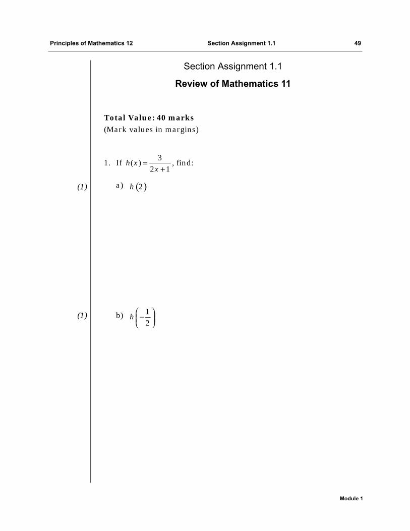
Section Assignment 1.1
Review of Mathematics 11
Total Value: 40 marks(Mark values in margins)
1. If , find:
a)
b) 12
h −
( )2h
3( )
2 1h x
x=
+
(1)
(1)
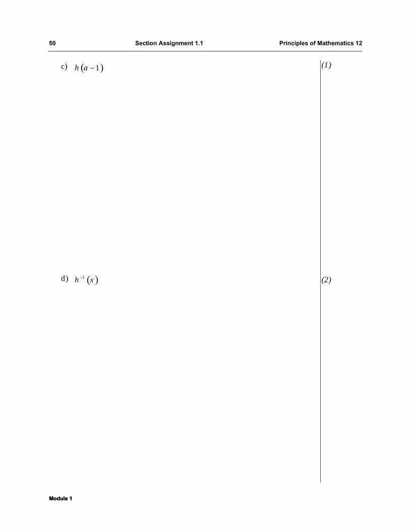
c)
d) ( )1h x−
( )1h a −
50 Section Assignment 1.1 Principles of Mathematics 12
Module 1Module 1
(1)
(2)
2. For the the function find:
a) the domain of g
b) the range of g
c) the y-intercept
d) the x-intercept
( ) 2 3g x x= +
Principles of Mathematics 12 Section Assignment 1.1 51
Module 1Module 1
(4)
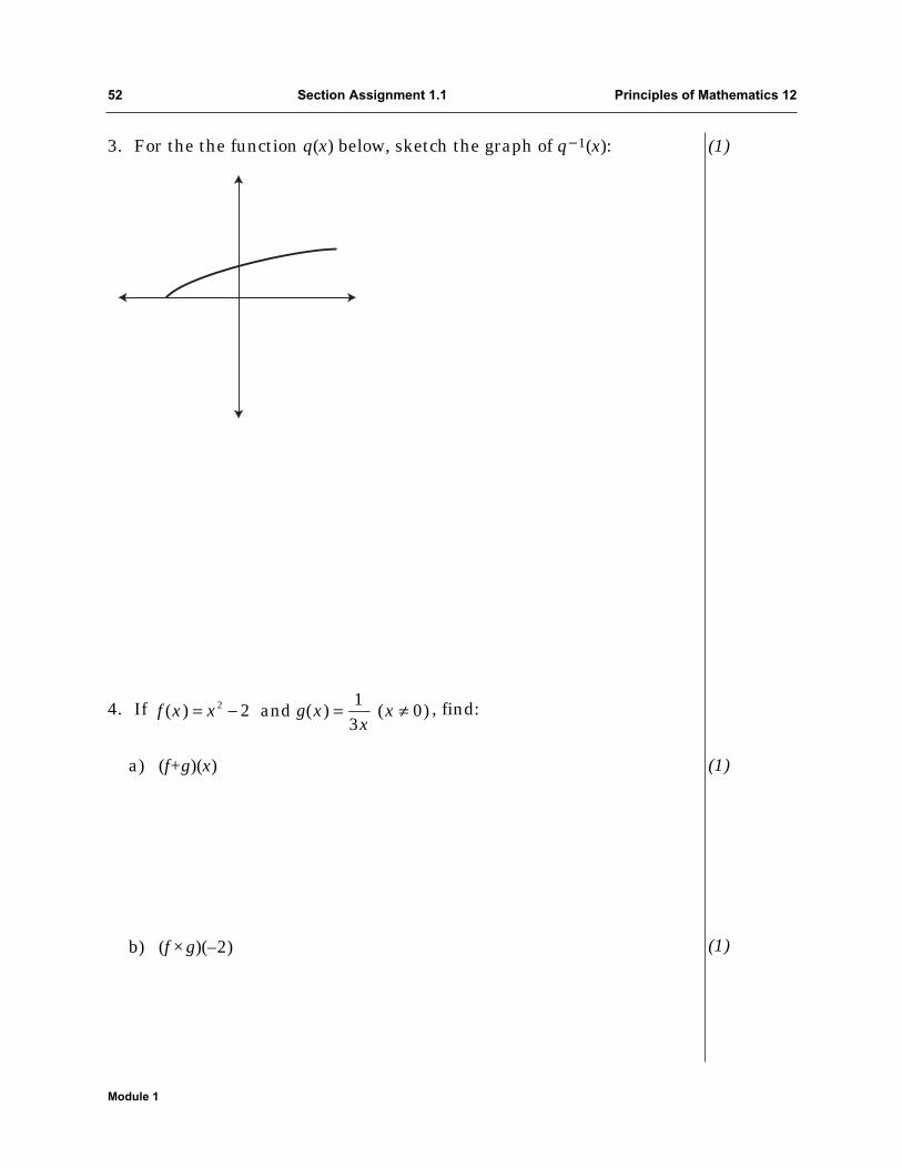
3. For the the function q(x) below, sketch the graph of q−1(x):
4. If , find:
a) (f+g)(x)
b) (f ×g)(–2)
2 1( ) 2 and ( ) ( 0)
3f x x g x x
x= − = ≠
52 Section Assignment 1.1 Principles of Mathematics 12
Module 1
(1)
(1)
(1)
c) f(g(x))
d) g(f(–1))
e) f–l(x) where x ≤ 0
5. Without using your graphing calculator, sketch the graph of g(x)= –2(x – 1)2(x + 3). Label the intercepts and give the domain andrange.
Principles of Mathematics 12 Section Assignment 1.1 53
Module 1
(5)
(1)
(1)
(2)
6. Given , find.f–l(x)
7. Find the maximum value of the function f(x) = –x4 – 3x2 + x + 7 anduse it to determine the range of f.
4( )
1x
f xx
−=+
54 Section Assignment 1.1 Principles of Mathematics 12
Module 1
(4)
(5)
8. Solve using your graphing calculator:
a) 2x4 – 3x3 = x
b)2
2
2 42 3x x
xx x
− − =+ −
Principles of Mathematics 12 Section Assignment 1.1 55
Module 1
(1)
(2)
9. Given:
Determine:
Send in this work as soon as you complete this section.
) ( ( ))
) ( (3))
) ( ( ( 1)))
a g h x
b f h
c h g f −
2
( ) 2
( ) 7
( ) 2 5
f x x
g x x
h x x
= +
= −
= −
56 Section Assignment 1.1 Principles of Mathematics 12
Module 1
(1)
(1)
(2)
Total: 37 marks