Module 1: SAS - Technical University of Denmarkperbb/st113/Module01/sas.pdf · 2011-08-23 · Module 1: SAS 1.1 Importing Data ... 1.3.2 Simple analysis by an ANOVA approach: Data

DTU InformaticsPREPARED BY THE STATISTICS GROUPS AT IMM, DTU AND KU-LIFE

02429/MIXED LINEAR MODELS

Module 1: SAS

1.1 Importing Data . . . . . . . . . . . . . . . . . . . . . . . . . . . . . 2

1.1.1 Creating a Library for the Data . . . . . . . . . . . . . . . . . 2

1.1.2 The Data-step . . . . . . . . . . . . . . . . . . . . . . . . . . 3

1.1.3 Importing Delimited Files . . . . . . . . . . . . . . . . . . . 3

1.1.4 Importing Microsoft Excel files . . . . . . . . . . . . . . . . 4

1.1.5 Downloading SAS data files . . . . . . . . . . . . . . . . . . 5

1.1.6 SAS JMP: Import of data files. . . . . . . . . . . . . . . . . . 5

1.2 Creating Graphs . . . . . . . . . . . . . . . . . . . . . . . . . . . . . 6

1.2.1 The GPLOT Procedure . . . . . . . . . . . . . . . . . . . . . 6

1.2.2 Using SAS Help . . . . . . . . . . . . . . . . . . . . . . . . 7

1.3 Introductory example: NIR predictions of HPLC measurements . . . 8

1.3.1 Simple analysis . . . . . . . . . . . . . . . . . . . . . . . . . 8

1.3.2 Simple analysis by an ANOVA approach: Data re-structuring 9

1.3.3 ANOVA approach: Using PROC GLM . . . . . . . . . . . . 10

1.3.4 ANOVA approach: LSMEANS . . . . . . . . . . . . . . . . 12

1.3.5 ANOVA approach: ESTIMATE . . . . . . . . . . . . . . . . 14

1.3.6 Analysis by mixed model . . . . . . . . . . . . . . . . . . . . 14

1.4 Example with missing values . . . . . . . . . . . . . . . . . . . . . . 17

1.4.1 Simple analysis by an ANOVA approach . . . . . . . . . . . 18

1.4.2 Analysis by mixed model . . . . . . . . . . . . . . . . . . . . 21

1.5 Conclusion . . . . . . . . . . . . . . . . . . . . . . . . . . . . . . . 23

02429/Mixed Linear Models http://www.imm.dtu.dk/courses/02429/ Last modified August 23, 2011

Module 1: SAS 2

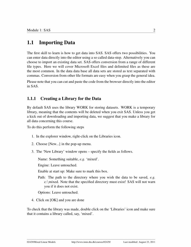
1.1 Importing Data

The first skill to learn is how to get data into SAS. SAS offers two possibilities. Youcan enter data directly into the editor using a so called data-step. Alternatively you canchoose to import an existing data set. SAS offers conversion from a range of differentfile types. Here we will cover Microsoft Excel files and delimited files as these arethe most common. In the data data base all data sets are stored as text separated withcommas. Conversion from other file formats are easy when you grasp the general idea.

Please note that you can cut and paste the code from the browser directly into the editorin SAS.

1.1.1 Creating a Library for the Data

By default SAS uses the library WORK for storing datasets. WORK is a temporarylibrary, meaning that the contents will be deleted when you exit SAS. Unless you geta kick out of downloading and importing data, we suggest that you make a library forall data concerning this course.

To do this perform the following steps

1. In the explorer window, right-click on the Libraries icon.

2. Choose [New...] in the pop-up menu.

3. The ‘New Library’ window opens – specify the fields as follows.

Name: Something suitable, e.g. ‘mixed’.

Engine: Leave untouched.

Enable at start up: Make sure to mark this box.

Path: The path to the directory where you wish the data to be saved, e.g.c:\mixed. Note that the specified directory must exist! SAS will not warnyou if it does not exist.

Options: Leave untouched.

4. Click on [OK] and you are done

To check that the library was made, double click on the ‘Libraries’ icon and make surethat it contains a library called, say, ‘mixed’.

02429/Mixed Linear Models http://www.imm.dtu.dk/courses/02429/ Last modified: August 23, 2011

Module 1: SAS 3

1.1.2 The Data-step

To prepare your data for analysis, you must create a SAS data set. In the DATA step,you can create data sets and manipulate your data with SAS programming statements:

data mixed.hplcnir1; /* The name of data set *//* mixed specifies the library *//* hplcnir1 will be the name of the data */

input hplc nir ; /* The name of the columns */datalines; /* Indicates that observations starts */10.4 10.10.6 10.810.2 10.210.1 9.910.3 1110.7 10.510.3 10.210.9 10.910.1 10.49.8 9.9run;

1.1.3 Importing Delimited Files

To perform the steps in this description you should download the dataset hplcnir1.txt.Place it somewhere where you can find it again.Below you see what the file looks like:

hplc,nir10.4,10.110.6,10.810.2,10.210.1,9.910.3,1110.7,10.510.3,10.210.9,10.910.1,10.49.8,9.9

This is the basic data format used throughout the course. To import the delimited fileinto SAS perform the following steps:

1. Choose [File→ Import Data].

2. In the pop-up window you should change ‘Microsoft Excel 97 or 2000 (*.xls)’to ‘Delimited File (*.*)’.


Module 1: SAS 4

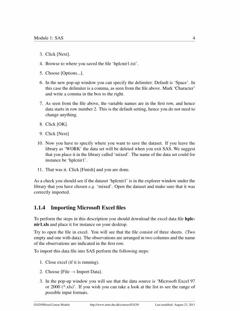
3. Click [Next].

4. Browse to where you saved the file ‘hplcnir1.txt’.

5. Choose [Options...].

6. In the new pop-up window you can specify the delimiter. Default is ‘Space’. Inthis case the delimiter is a comma, as seen from the file above. Mark ‘Character’and write a comma in the box to the right.

7. As seen from the file above, the variable names are in the first row, and hencedata starts in row number 2. This is the default setting, hence you do not need tochange anything.

8. Click [OK].

9. Click [Next]

10. Now you have to specify where you want to save the dataset. If you leave thelibrary as ‘WORK’ the data set will be deleted when you exit SAS. We suggestthat you place it in the library called ‘mixed’. The name of the data set could forinstance be ‘hplcnir1’.

11. That was it. Click [Finish] and you are done.

As a check you should see if the dataset ‘hplcnir1’ is in the explorer window under thelibrary that you have chosen e.g. ‘mixed’. Open the dataset and make sure that it wascorrectly imported.

1.1.4 Importing Microsoft Excel files

To perform the steps in this description you should download the excel data file hplc-nir1.xls and place it for instance on your desktop.

Try to open the file in excel. You will see that the file consist of three sheets. (Twoempty and one with data). The observations are arranged in two columns and the nameof the observations are indicated in the first row.

To import this data file into SAS perform the following steps:

1. Close excel (if it is running).

2. Choose [File→ Import Data].

3. In the pop-up window you will see that the data source is ‘Microsoft Excel 97or 2000 (*.xls)’. If you wish you can take a look at the list to see the range ofpossible input formats.


Module 1: SAS 5

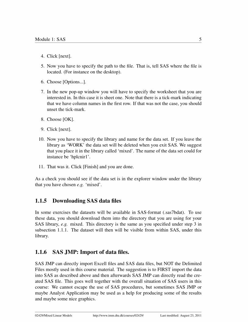
4. Click [next].

5. Now you have to specify the path to the file. That is, tell SAS where the file islocated. (For instance on the desktop).

6. Choose [Options...].

7. In the new pop-up window you will have to specify the worksheet that you areinterested in. In this case it is sheet one. Note that there is a tick-mark indicatingthat we have column names in the first row. If that was not the case, you shouldunset the tick-mark.

8. Choose [OK].

9. Click [next].

10. Now you have to specify the library and name for the data set. If you leave thelibrary as ‘WORK’ the data set will be deleted when you exit SAS. We suggestthat you place it in the library called ‘mixed’. The name of the data set could forinstance be ‘hplcnir1’.

11. That was it. Click [Finish] and you are done.

As a check you should see if the data set is in the explorer window under the librarythat you have chosen e.g. ‘mixed’.

1.1.5 Downloading SAS data files

In some exercises the datasets will be available in SAS-format (.sas7bdat). To usethese data, you should download them into the directory that you are using for yourSAS library, e.g. mixed. This directory is the same as you specified under step 3 insubsection 1.1.1. The dataset will then will be visible from within SAS, under thislibrary.

1.1.6 SAS JMP: Import of data files.

SAS JMP can directly import Excell files and SAS data files, but NOT the DelimitedFiles mostly used in this course material. The suggestion is to FIRST import the datainto SAS as described above and then afterwards SAS JMP can directly read the cre-ated SAS file. This goes well together with the overall situation of SAS users in thiscourse: We cannot escape the use of SAS procedures, but sometimes SAS JMP ormaybe Analyst Application may be used as a help for producing some of the resultsand maybe some nice graphics.


Module 1: SAS 6

1.2 Creating Graphs

Now you have successfully created a SAS dataset.

The next step is to visualize the data in a scatter-plot. To this we recommend theprocedure GPLOT which is described in the following.

1.2.1 The GPLOT Procedure

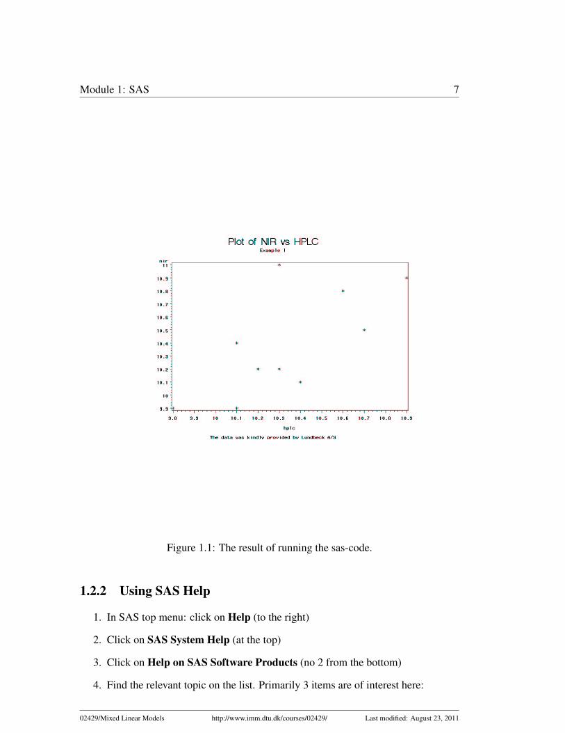
The GPLOT procedure produces two-dimensional graphs that plot one variable againstanother within a set of coordinate axes. The coordinates of each point on the plotcorrespond to two variable values in an observation of the input data set. Graphs areautomatically scaled to the values of your data. If you wish you may rescale the axisusing the AXIS statements.7Before looking at the syntax of the PROC GPLOT procedure, we set some variables.The meaning of these will be obvious when you look at the plot.

title1 ’Plot of NIR vs HPLC’;title2 ’Example 1’;footnote ’The data was kindly provided by Lundbeck A/S’;

The basic GPLOT statement looks like this

proc gplot data=mixed.hplcnir1; /* the data you wish to plot */plot NIR*HPLC; /* The variables in format y*x */symbol value=star i=RL; /* The symbol for the points AND: */

run; /* i=RL means: Interpolation should*/quit; /* be done by a Linear(L) Regression(R)*/title1; /* Resets the title and footnote contents to */title2; /* avoid that these are used for */footnote; /* following output and plots */

It produces the plot in figure 1.1

In Module 3 further details on using PROC GPLOT is given. For a complete descrip-tion and list of options, use the SAS help menu.

Scatter plots in SAS JMP

Use ”Graph”, ”Overlay Plot”.


Module 1: SAS 7

Figure 1.1: The result of running the sas-code.

1.2.2 Using SAS Help

1. In SAS top menu: click on Help (to the right)

2. Click on SAS System Help (at the top)

3. Click on Help on SAS Software Products (no 2 from the bottom)

4. Find the relevant topic on the list. Primarily 3 items are of interest here:


Module 1: SAS 8

• Base SAS (Offering help on basic SAS Language, basic SAS procedureincluding data handling.

• SAS/GRAPH (Offering help on graphics including GPLOT and the useof SYMBOL and AXIS statements to control the graphics)

• SAS/STAT (Offering help on all statistical procedures)

Note that it is possible to add favorites in line with web-browsing making future find-ings of relevant help information much easier.

1.3 Introductory example: NIR predictions of HPLCmeasurements

In this section we go through the steps needed to do the calculations given in theintroductory example.

1.3.1 Simple analysis

This is most easily carried out by constructing the difference as a new variable in thedata set, and then using a basic SAS procedure, for instance PROC UNIVARIATE.Before doing this, it is a good idea to change the line size that SAS uses for the OUT-PUT:

options ls=68 ps=40; /* Line size in OUTPUT set to 68 characters */title ’Example 1, NIR/HPLC data’; /* title for the OUTPUT */data temp; /* Creates a new data set named "temp" */set mixed.hplcnir1; /* as a copy of the hplcnir1 data set */d=hplc-nir; /* The new difference variable "d" is created*/run;proc univariate all; /* All summary statistics are requested for */var d; /* variable d */run;

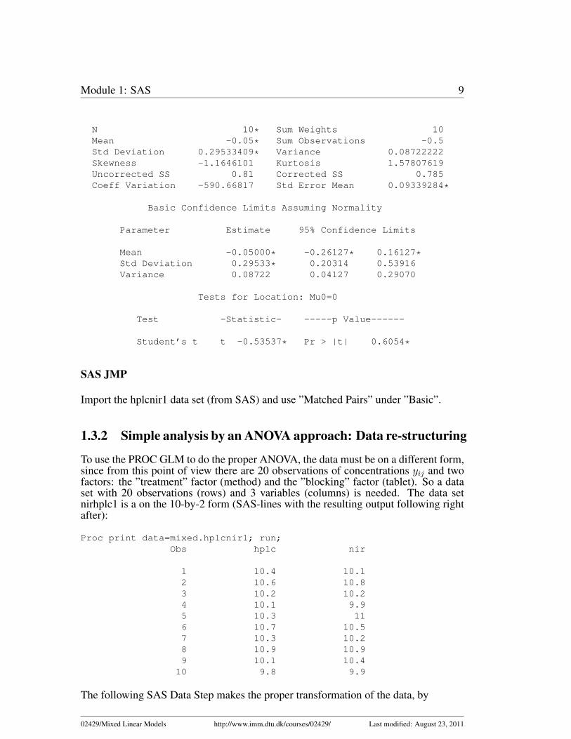
Among a large amount of output information the following bits can be found, thatprovide all the results of the simple analysis:(A star ”*” was added to the numbers alsofound in the example computations)

Example 1, NIR/HPLC data

The UNIVARIATE ProcedureVariable: d

Moments


Module 1: SAS 9

N 10* Sum Weights 10Mean -0.05* Sum Observations -0.5Std Deviation 0.29533409* Variance 0.08722222Skewness -1.1646101 Kurtosis 1.57807619Uncorrected SS 0.81 Corrected SS 0.785Coeff Variation -590.66817 Std Error Mean 0.09339284*

Basic Confidence Limits Assuming Normality

Parameter Estimate 95% Confidence Limits

Mean -0.05000* -0.26127* 0.16127*Std Deviation 0.29533* 0.20314 0.53916Variance 0.08722 0.04127 0.29070

Tests for Location: Mu0=0

Test -Statistic- -----p Value------

Student’s t t -0.53537* Pr > |t| 0.6054*

SAS JMP

Import the hplcnir1 data set (from SAS) and use ”Matched Pairs” under ”Basic”.

1.3.2 Simple analysis by an ANOVA approach: Data re-structuring

To use the PROC GLM to do the proper ANOVA, the data must be on a different form,since from this point of view there are 20 observations of concentrations yij and twofactors: the ”treatment” factor (method) and the ”blocking” factor (tablet). So a dataset with 20 observations (rows) and 3 variables (columns) is needed. The data setnirhplc1 is a on the 10-by-2 form (SAS-lines with the resulting output following rightafter):

Proc print data=mixed.hplcnir1; run;Obs hplc nir

1 10.4 10.12 10.6 10.83 10.2 10.24 10.1 9.95 10.3 116 10.7 10.57 10.3 10.28 10.9 10.99 10.1 10.410 9.8 9.9

The following SAS Data Step makes the proper transformation of the data, by


Module 1: SAS 10

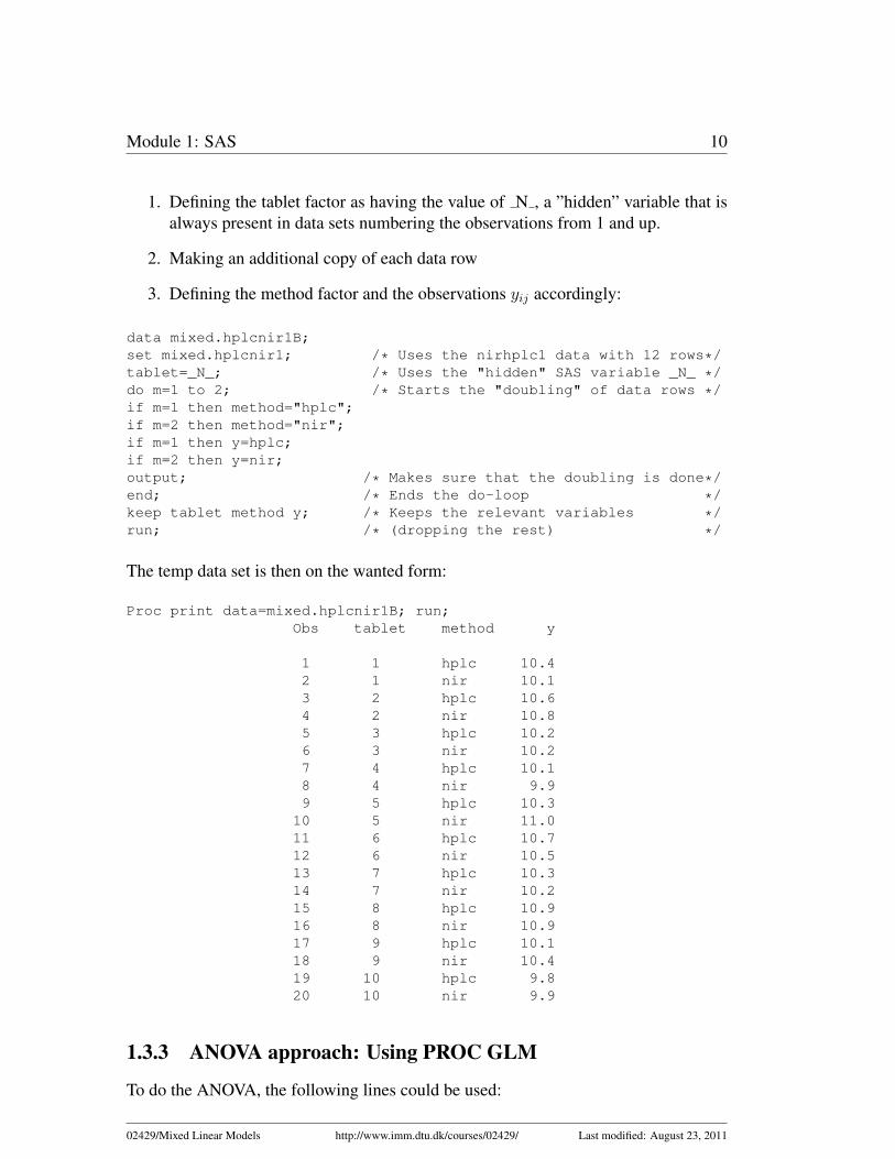
1. Defining the tablet factor as having the value of N , a ”hidden” variable that isalways present in data sets numbering the observations from 1 and up.

2. Making an additional copy of each data row

3. Defining the method factor and the observations yij accordingly:

data mixed.hplcnir1B;set mixed.hplcnir1; /* Uses the nirhplc1 data with 12 rows*/tablet=_N_; /* Uses the "hidden" SAS variable _N_ */do m=1 to 2; /* Starts the "doubling" of data rows */if m=1 then method="hplc";if m=2 then method="nir";if m=1 then y=hplc;if m=2 then y=nir;output; /* Makes sure that the doubling is done*/end; /* Ends the do-loop */keep tablet method y; /* Keeps the relevant variables */run; /* (dropping the rest) */

The temp data set is then on the wanted form:

Proc print data=mixed.hplcnir1B; run;Obs tablet method y

1 1 hplc 10.42 1 nir 10.13 2 hplc 10.64 2 nir 10.85 3 hplc 10.26 3 nir 10.27 4 hplc 10.18 4 nir 9.99 5 hplc 10.3

10 5 nir 11.011 6 hplc 10.712 6 nir 10.513 7 hplc 10.314 7 nir 10.215 8 hplc 10.916 8 nir 10.917 9 hplc 10.118 9 nir 10.419 10 hplc 9.820 10 nir 9.9

1.3.3 ANOVA approach: Using PROC GLM

To do the ANOVA, the following lines could be used:


Module 1: SAS 11

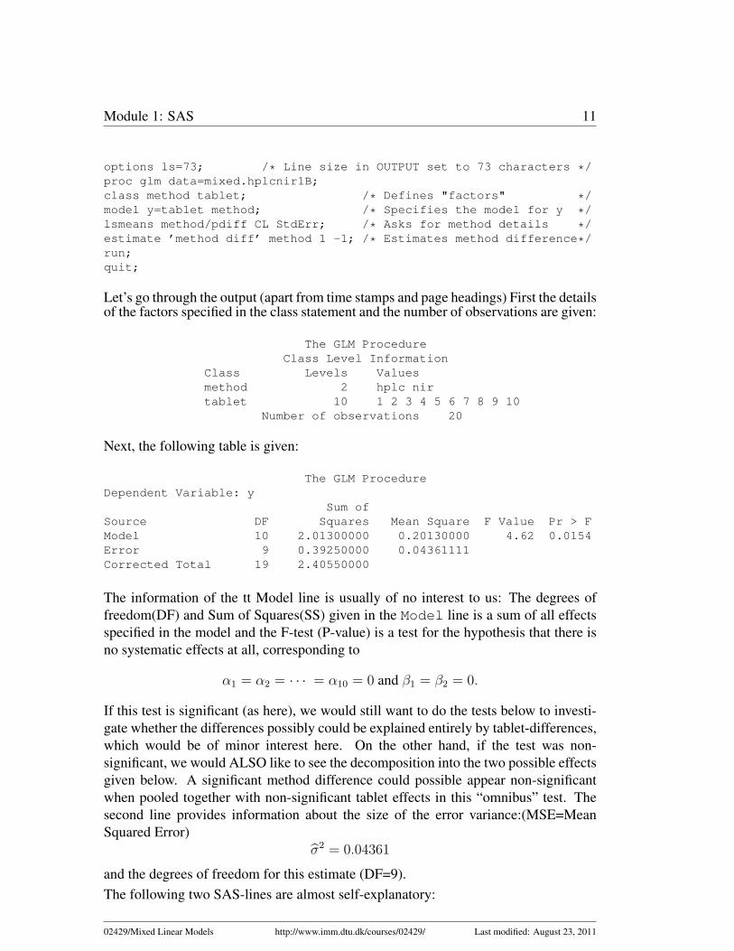
options ls=73; /* Line size in OUTPUT set to 73 characters */proc glm data=mixed.hplcnir1B;class method tablet; /* Defines "factors" */model y=tablet method; /* Specifies the model for y */lsmeans method/pdiff CL StdErr; /* Asks for method details */estimate ’method diff’ method 1 -1; /* Estimates method difference*/run;quit;

Let’s go through the output (apart from time stamps and page headings) First the detailsof the factors specified in the class statement and the number of observations are given:

The GLM ProcedureClass Level Information

Class Levels Valuesmethod 2 hplc nirtablet 10 1 2 3 4 5 6 7 8 9 10

Number of observations 20

Next, the following table is given:

The GLM ProcedureDependent Variable: y

Sum ofSource DF Squares Mean Square F Value Pr > FModel 10 2.01300000 0.20130000 4.62 0.0154Error 9 0.39250000 0.04361111Corrected Total 19 2.40550000

The information of the tt Model line is usually of no interest to us: The degrees offreedom(DF) and Sum of Squares(SS) given in the Model line is a sum of all effectsspecified in the model and the F-test (P-value) is a test for the hypothesis that there isno systematic effects at all, corresponding to

α1 = α2 = · · · = α10 = 0 and β1 = β2 = 0.

If this test is significant (as here), we would still want to do the tests below to investi-gate whether the differences possibly could be explained entirely by tablet-differences,which would be of minor interest here. On the other hand, if the test was non-significant, we would ALSO like to see the decomposition into the two possible effectsgiven below. A significant method difference could possible appear non-significantwhen pooled together with non-significant tablet effects in this “omnibus” test. Thesecond line provides information about the size of the error variance:(MSE=MeanSquared Error)

σ̂2 = 0.04361

and the degrees of freedom for this estimate (DF=9).The following two SAS-lines are almost self-explanatory:


Module 1: SAS 12

R-Square Coeff Var Root MSE y Mean

0.836832 2.014788 0.208833 10.36500

R-square is sometimes called the coefficient of determination:

R2 = 1− SSError

SSTotal

=SSModel

SSTotal

and expresses the amount of variation in y explained by the model. The Coefficientof Variation is the ratio (in percentage) between the residual standard deviation (RootMSE) and the mean of y and expresses the level of residual variability relative to thesize of y.

The ANOVA table(s) comes next: (Exactly reproducing the ANOVA table given in theintroductory example):

Source DF Type I SS Mean Square F Value Pr > F

tablet 9 2.00050000 0.22227778 5.10 0.0118method 1 0.01250000 0.01250000 0.29 0.6054

Source DF Type III SS Mean Square F Value Pr > F

tablet 9 2.00050000 0.22227778 5.10 0.0118method 1 0.01250000 0.01250000 0.29 0.6054

By default, SAS prints out two ANOVA tables, the Type I and the Type III table. Whenthe data is ”balanced” (in this case meaning no missing observations) these two tablesare the same, as here: there is a unique decomposition of the total variability(sums ofsquares) into the three components:

SSTotal = SStablet + SSmethod + SSerror.

Only in cases where such a unique explanation of the reasons for the variability in thedata does not exist, the two tables will differ. In the missing data example below thedifference between Type I and Type III tables will be further explained. In any case,the mean squares measure the differences in the data induced by the various effects.For instance, a main effect mean square expresses the variation between the means forthe different levels of the factor.

SAS JMP

Import the hplcnir1B data set (from SAS) and use ”Fit Model”. Add both tablet andmethod as model effects (make sure that tablet is set to nominal modelling type).


Module 1: SAS 13

1.3.4 ANOVA approach: LSMEANS

The LSMEANS statement used provided the following information about the methods:

The GLM ProcedureLeast Squares Means

H0:LSMean1=Standard H0:LSMEAN=0 LSMean2

method y LSMEAN Error Pr > |t| Pr > |t|

hplc 10.3400000 0.0660387 <.0001 0.6054nir 10.3900000 0.0660387 <.0001

method y LSMEAN 95% Confidence Limits

hplc 10.340000 10.190610 10.489390nir 10.390000 10.240610 10.539390

Formally, LSMEANS (Least Squares Means) are model estimates of the expected val-ues for the two methods:

µ̂+ β̂1 + ¯̂α = 10.34

µ̂+ β̂2 + ¯̂α = 10.39

where ¯̂α is the average of the 10 tablet contribution parameters. In this case, this is ex-actly the same as the simple means of the data within each method, that could be givenusing the MEANS statement of PROC GLM. For unbalanced data, situations with co-variates or mixed models in general, the parameter estimates will in general NOT begiven by simple averages of the data, and the use of LSMEANS is generally advisable.The standard errors (uncertainties) are given next (because of the option STDERR).Note that in this case these standard errors should NOT be used! The t-test for thehypothesis that LSMEAN=0, which is always provided by the LSMEANS statement,is rarely of interest: It is an irrelevant hypothesis in most cases. The following testfor the differences (provided because of the option PDIFF) is the relevant test: Notethat the P-value of this t-test (0.6054) equals the P-value for the F-test. Next the 95%confidence limits for the LSMEANS are given (because of the option CL). Since theseare based on the incorrect standard errors, they should NOT be used either.The final consequence of the LSMEANS statement is the estimate for the methoddifference together with a 95% confidence interval for this:

Least Squares Means for Effect method

DifferenceBetween 95% Confidence Limits for

i j Means LSMean(i)-LSMean(j)

1 2 -0.050000 -0.261269 0.161269


Module 1: SAS 14

SAS JMP

The LSmeans information for methods is a part or the SAS JMP output, althoughthe Confidence intervals for each of the LSmeans are not explicitly given (only thestandard errors). The LSmeans difference and confidence interval is given explicitly:Go to the result window, click the menu down at ”method”, click ”LSMeans student’st”.

1.3.5 ANOVA approach: ESTIMATE

Finally, the ESTIMATE statement was used:

estimate ’method diff’ method 1 -1;

With this statement any (estimable) linear combination of the parameters

a1β1 + a2β2

can be estimated (together with it’s uncertainty). Choosing 1 and −1 yields the simpledifference and it’s standard error, as also given in the main text of this module:

The GLM ProcedureDependent Variable: y

StandardParameter Estimate Error t Value Pr > |t|

method diff -0.05000000 0.09339284 -0.54 0.6054

1.3.6 Analysis by mixed model

The proper mixed model analysis can be performed by the PROCEDURE MIXED:

proc mixed data=hplcnir1b;class method tablet; /* Defines all "factors" */model y=method/DDFM=satterth; /* Specifies the fixed effects */lsmeans method/pdiff CL; /* Asks for method details */estimate ’method diff’ method 1 -1; /* Estimates method difference */random tablet; /* Specifies the random effects*/run;quit;

The main difference to the use of PROC GLM is that only fixed effects are to be listedin the MODEL statement, and then random effects should be listed in the RANDOMstatement. Secondly, there are some differences in the choice of (and need for) thedifferent options. No details are given at this state.The first part of the OUTPUT summarizes data, factor and model information, togetherwith some details on ”model fit”, that we will return to in Module 3:


Module 1: SAS 15

The Mixed Procedure

Model Information

Data Set WORK.TEMPDependent Variable yCovariance Structure Variance ComponentsEstimation Method REMLResidual Variance Method ProfileFixed Effects SE Method Model-BasedDegrees of Freedom Method Satterthwaite

Class Level Information

Class Levels Values

method 2 hplc nirtablet 10 1 2 3 4 5 6 7 8 9 10

Dimensions

Covariance Parameters 2Columns in X 3Columns in Z 10Subjects 1Max Obs Per Subject 20Observations Used 20Observations Not Used 0Total Observations 20

Iteration History

Iteration Evaluations -2 Res Log Like Criterion

0 1 19.366126301 1 13.96052066 0.00000000

Convergence criteria met.

Covariance ParameterEstimates

Cov Parm Estimate

tablet 0.08933Residual 0.04361


Module 1: SAS 16

Fit Statistics

-2 Res Log Likelihood 14.0AIC (smaller is better) 18.0AICC (smaller is better) 18.8BIC (smaller is better) 18.6

Note, however, the ”Covariance Parameter Estimates” headline. This is where theestimates of the unknowns (parameters) of the random part of the model are given. Werecognize the estimates for the two variance components:

σ̂2T = 0.0894

σ̂2 = 0.0436

Next, (parts of) the ANOVA table for the fixed effects of the model is given:

Type 3 Tests of Fixed Effects

Num DenEffect DF DF F Value Pr > F

method 1 9 0.29 0.6054

Often this will contain the important overall test information. The results of the ESTI-MATE statement follows:

The Mixed Procedure

EstimatesStandard

Label Estimate Error DF t Value Pr > |t|

method diff -0.05000 0.09339 9 -0.54 0.6054

and finally the results of the LSMEANS statement:

Least Squares Means

StandardEffect method Estimate Error DF t Value Pr > |t| Alpha

method hplc 10.3400 0.1153 12.4 89.68 <.0001 0.05method nir 10.3900 0.1153 12.4 90.11 <.0001 0.05

Least Squares Means

Effect method Lower Upper


Module 1: SAS 17

method hplc 10.0897 10.5903method nir 10.1397 10.6403

Differences of Least Squares Means

StandardEffect method _method Estimate Error DF t Value Pr > |t|

method hplc nir -0.05000 0.09339 9 -0.54 0.6054

Note that the standard errors (now given automatically without any option) for theLSMEANS have changed. Otherwise, the information is comparable in structure andcontent to the PROC GLM output.

SAS JMP

The only thing needed as compared to running the two-way additive fixed effect ANOVAin SAS JMP as described above, is to specify the tablet model effect as random: In themodel effect list, mark the tablet effect and then click ”attributes” and ”random ef-fects”.

1.4 Example with missing values

In this section we go through the steps needed to do the calculations given in theintroductory example with missing values. The SAS-lines needed can be copiedfrom above (with suitable change of file-names):

data mixed.hplcnir2B;set mixed.hplcnir2;tablet=_N_;do m=1 to 2;if m=1 then method="hplc";if m=2 then method="nir";if m=1 then y=hplc;if m=2 then y=nir;output;end;keep tablet method y;run;Proc print data=temp2; run;

The print procedure yields the data listing in the output:

Example 1, NIR/HPLC dataObs tablet method y


Module 1: SAS 18

1 1 hplc 10.42 1 nir 10.13 2 hplc 10.64 2 nir 10.85 3 hplc 10.26 3 nir 10.27 4 hplc 10.18 4 nir 9.99 5 hplc 10.310 5 nir 11.011 6 hplc 10.712 6 nir 10.513 7 hplc 10.314 7 nir 10.215 8 hplc 10.916 8 nir 10.917 9 hplc 10.118 9 nir 10.419 10 hplc 9.820 10 nir 9.921 11 hplc .22 11 nir 10.823 12 hplc .24 12 nir 9.825 13 hplc .26 13 nir 10.527 14 hplc .28 14 nir 10.329 15 hplc .30 15 nir 9.731 16 hplc 10.332 16 nir .33 17 hplc 9.634 17 nir .35 18 hplc 10.036 18 nir .37 19 hplc 10.238 19 nir .39 20 hplc 9.940 20 nir .

Note that SAS uses a dot ”.” as code for a missing observation.

1.4.1 Simple analysis by an ANOVA approach

The copies of the SAS-lines needed are then:

proc glm data=mixed.hplcnir2B;


Module 1: SAS 19

class method tablet; /* Defines "factors" */model y=tablet method; /* Specifies the model for y */lsmeans method/pdiff CL StdErr; /* Asks for method details */estimate ’method diff’ method 1 -1; /* Estimates method difference*/run;quit;

The PROC GLM output is:

The GLM Procedure


Class Levels Values

method 2 hplc nir

tablet 20 1 2 3 4 5 6 7 8 9 10 11 12 13 14 15 16 17 18 19 20

Number of observations 40

NOTE: Due to missing values, only 30 observations can be used in thisanalysis.

The GLM Procedure

Dependent Variable: y

Sum ofSource DF Squares Mean Square F Value Pr > F

Model 20 3.73550000 0.18677500 4.28 0.0149

Error 9 0.39250000 0.04361111

Corrected Total 29 4.12800000

R-Square Coeff Var Root MSE y Mean

0.904918 2.031447 0.208833 10.28000

Source DF Type I SS Mean Square F Value Pr > F

tablet 19 3.72300000 0.19594737 4.49 0.0129method 1 0.01250000 0.01250000 0.29 0.6054

Source DF Type III SS Mean Square F Value Pr > F


Module 1: SAS 20

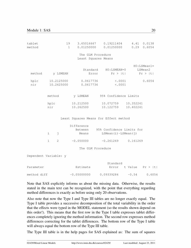
tablet 19 3.65016667 0.19211404 4.41 0.0138method 1 0.01250000 0.01250000 0.29 0.6054

The GLM ProcedureLeast Squares Means

H0:LSMean1=Standard H0:LSMEAN=0 LSMean2

method y LSMEAN Error Pr > |t| Pr > |t|

hplc 10.2125000 0.0617736 <.0001 0.6054nir 10.2625000 0.0617736 <.0001

method y LSMEAN 95% Confidence Limits

hplc 10.212500 10.072759 10.352241nir 10.262500 10.122759 10.402241

Least Squares Means for Effect method

DifferenceBetween 95% Confidence Limits for

i j Means LSMean(i)-LSMean(j)

1 2 -0.050000 -0.261269 0.161269

The GLM Procedure

Dependent Variable: y

StandardParameter Estimate Error t Value Pr > |t|

method diff -0.05000000 0.09339284 -0.54 0.6054

Note that SAS explicitly informs us about the missing data. Otherwise, the resultsstated in the main text can be recognized, with the point that everything regardingmethod differences is exactly as before using only 20 observations.

Also note that now the Type I and Type III tables are no longer exactly equal. TheType I table provides a successive decomposition of the total variability in the orderthat the effects were typed in the MODEL statement (so the results shown depend onthis order!). This means that the first row in the Type I table expresses tablet differ-ences completely ignoring the method information. The second row expresses methoddifferences correcting for the tablet differences. The bottom row of the Type I tablewill always equal the bottom row of the Type III table.

The Type III table is in the help pages for SAS explained as: The sum of squares


Module 1: SAS 21

for each term represents the variation among the means for the different levels of thefactors. The Type III Tests table presents the Type III sums of squares associatedwith the effects in the model. The Type III sum of squares for a particular effect isthe amount of variation in the response due to that effect after correcting for all otherterms in the model. Type III sums of squares, therefore, do not depend on the order inwhich the effects are specified in the model. Refer to the chapter on ”The Four Typesof Estimable Functions,” in the SAS/STAT User’s Guide for a complete discussion ofType I -IV sums of squares.

The correction for method difference has no effect if all tablets were measured by bothmethods, but since this is not the case the correction will (slightly) change the resulthere.

1.4.2 Analysis by mixed model

The SAS-lines for the mixed model analysis are:

proc mixed data=mixed.hplcnir2B;class method tablet; /* Defines all "factors" */model y=method/DDFM=satterth; /* Specifies the fixed effects */lsmeans method/pdiff CL; /* Asks for method details */estimate ’method diff’ method 1 -1; /* Estimates method difference */random tablet; /* Specifies the random effects*/run;quit;

The output giving the stated results is:

The Mixed Procedure

Model Information

Data Set WORK.TEMP2Dependent Variable yCovariance Structure Variance ComponentsEstimation Method REMLResidual Variance Method ProfileFixed Effects SE Method Model-BasedDegrees of Freedom Method Satterthwaite


Class Levels Values

method 2 hplc nirtablet 20 1 2 3 4 5 6 7 8 9 10 11 12 13

14 15 16 17 18 19 20


Module 1: SAS 22

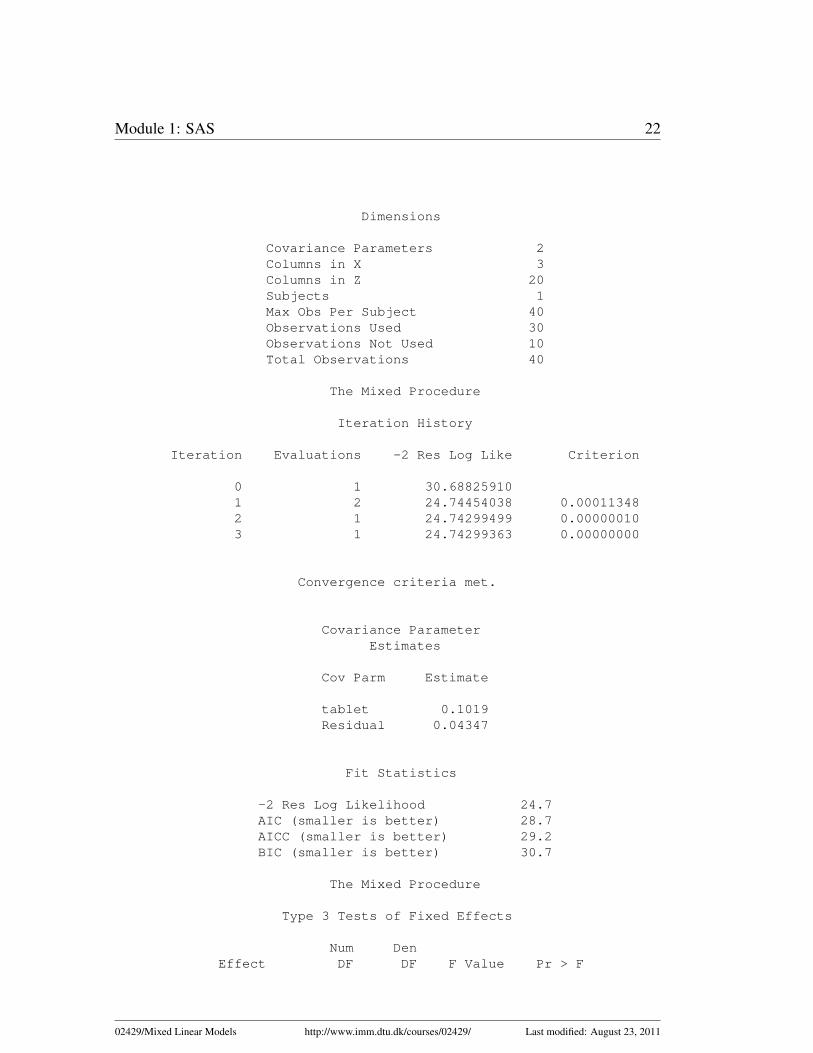
Dimensions

Covariance Parameters 2Columns in X 3Columns in Z 20Subjects 1Max Obs Per Subject 40Observations Used 30Observations Not Used 10Total Observations 40

The Mixed Procedure

Iteration History

Iteration Evaluations -2 Res Log Like Criterion

0 1 30.688259101 2 24.74454038 0.000113482 1 24.74299499 0.000000103 1 24.74299363 0.00000000

Convergence criteria met.

Covariance ParameterEstimates

Cov Parm Estimate

tablet 0.1019Residual 0.04347

Fit Statistics

-2 Res Log Likelihood 24.7AIC (smaller is better) 28.7AICC (smaller is better) 29.2BIC (smaller is better) 30.7

The Mixed Procedure

Type 3 Tests of Fixed Effects

Num DenEffect DF DF F Value Pr > F


Module 1: SAS 23

method 1 11.7 0.69 0.4236

Estimates

StandardLabel Estimate Error DF t Value Pr > |t|

method diff -0.07211 0.08697 11.7 -0.83 0.4236

Least Squares Means

StandardEffect method Estimate Error DF t Value Pr > |t| Alpha

method hplc 10.2117 0.09259 25.8 110.29 <.0001 0.05method nir 10.2839 0.09259 25.8 111.07 <.0001 0.05

Least Squares Means

Effect method Lower Upper

method hplc 10.0214 10.4021method nir 10.0935 10.4743

The Mixed Procedure


StandardEffect method _method Estimate Error DF t Value Pr > |t|

method hplc nir -0.07211 0.08697 11.7 -0.83 0.4236


Effect method _method Alpha Lower Upper

method hplc nir 0.05 -0.2622 0.1179

1.5 Conclusion

You should now be able to solve the exercises for this module using SAS.


Documents

Module 1: SAS - Technical University of Denmarkperbb/st113/Module01/sas.pdf · 2011-08-23 · Module 1: SAS 1.1 Importing Data ... 1.3.2 Simple analysis by an ANOVA approach: Data