MODULE 3: GREISEN ALTERATION (PART I)tdb.mines.edu/Tutorials/Module3.pdfMODULE 3: GREISEN ALTERATION (PART I) In this tutorial we will use the GEMS project le "Module3" in the examples

GEMS Tutorial, A. Gysi, D. Kulik and D. Miron August 2018

MODULE 3: GREISEN ALTERATION (PART I)In this tutorial we will use the GEMS project file ”Module3” in the examples to

model the reaction path of a leucogranite during greisenization and evaluate the sol-ubility of Sn. We will learn how to: a) create Predefined Composition Objects (arock or fluid composition), b) add new minerals or aqueous species to your thermody-namic database and c) model more complex fluid-rock interaction processes (titration,multi-pass and leaching models). The example follows a modeling study of the EastKemptville tin deposit from Halter et al. (1998), Chem. Geol. 150, 1-17.

Create custom rock (Rock1) and fluid (Fluid1) compositions

1. Copy the folder Module3 to your project folder located in Library\Gems3\projects.

2. Open GEMS, choose the project and switch to the Thermodynamic Database

Mode and select in Panel 2 the option Compos for creating a predefined composi-tion object (PCO). The user interface is shown in Figure 1.

Fig. 1: GEMS user interface in Thermodynamic Database Mode. For adding a fluid or a rock chooseCompos in Panel 2. For adding a mineral and/or aqueous species to your database choose DComp orReacDC in Panel 2.

1


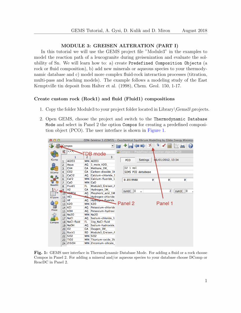
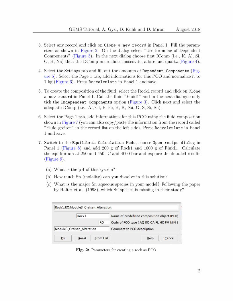
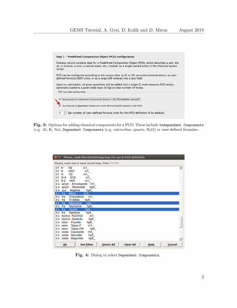
3. Select any record and click on Clone a new record in Panel 1. Fill the param-eters as shown in Figure 2. On the dialog select ”Use formulae of DependentComponents” (Figure 3). In the next dialog choose first IComp (i.e., K, Al, Si,O, H, Na) then the DComp microcline, muscovite, albite and quartz (Figure 4).

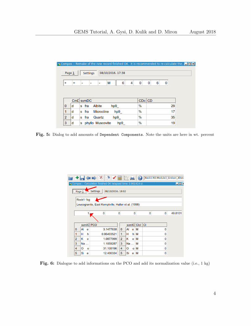
4. Select the Settings tab and fill out the amounts of Dependent Components (Fig-ure 5). Select the Page 1 tab, add informations for this PCO and normalize it to1 kg (Figure 6). Press Re-calculate in Panel 1 and save.

5. To create the composition of the fluid, select the Rock1 record and click on Clone

a new record in Panel 1. Call the fluid ”Fluid1” and in the next dialogue onlytick the Independent Components option (Figure 3). Click next and select theadequate IComp (i.e., Al, Cl, F, Fe, H, K, Na, O, S, Si, Sn).

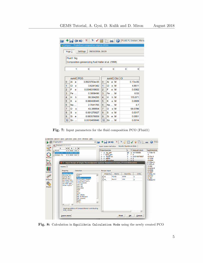
6. Select the Page 1 tab, add informations for this PCO using the fluid compositionshown in Figure 7 (you can also copy/paste the information from the record called”Fluid greisen” in the record list on the left side). Press Re-calculate in Panel1 and save.

7. Switch to the Equilibria Calculation Mode, choose Open recipe dialog inPanel 1 (Figure 8) and add 200 g of Rock1 and 1000 g of Fluid1. Calculatethe equilibrium at 250 and 450 ◦C and 4000 bar and explore the detailed results(Figure 9).

(a) What is the pH of this system?

(b) How much Sn (molality) can you dissolve in this solution?

(c) What is the major Sn aqueous species in your model? Following the paperby Halter et al. (1998), which Sn species is missing in their study?

Fig. 2: Parameters for creating a rock as PCO

2


Fig. 3: Options for adding chemical components for a PCO. These include Independent Components

(e.g. Al, K, Na), Dependent Components (e.g. microcline, quartz, H2O) or user-defined formulae.

Fig. 4: Dialog to select Dependent Components.

3


Fig. 5: Dialog to add amounts of Dependent Components. Note the units are here in wt. percent

Fig. 6: Dialogue to add informations on the PCO and add its normalization value (i.e., 1 kg)

4


Fig. 7: Input parameters for the fluid composition PCO (Fluid1)

Fig. 8: Calculation in Equilibria Calculation Mode using the newly created PCO

5


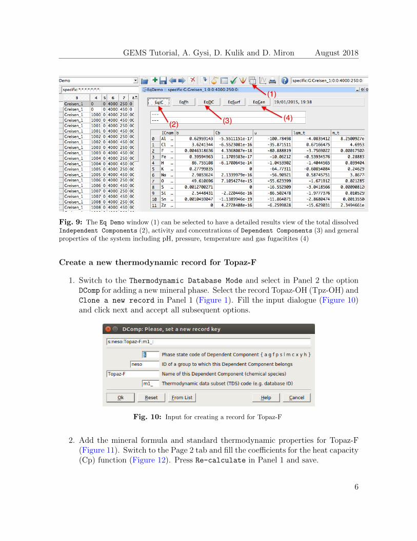
Fig. 9: The Eq Demo window (1) can be selected to have a detailed results view of the total dissolvedIndependent Components (2), activity and concentrations of Dependent Components (3) and generalproperties of the system including pH, pressure, temperature and gas fugacitites (4)

Create a new thermodynamic record for Topaz-F

1. Switch to the Thermodynamic Database Mode and select in Panel 2 the optionDComp for adding a new mineral phase. Select the record Topaz-OH (Tpz-OH) andClone a new record in Panel 1 (Figure 1). Fill the input dialogue (Figure 10)and click next and accept all subsequent options.

Fig. 10: Input for creating a record for Topaz-F

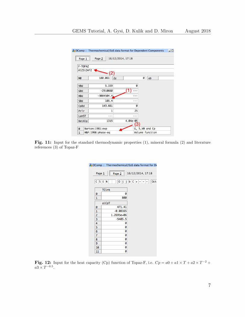
2. Add the mineral formula and standard thermodynamic properties for Topaz-F(Figure 11). Switch to the Page 2 tab and fill the coefficients for the heat capacity(Cp) function (Figure 12). Press Re-calculate in Panel 1 and save.

6


Fig. 11: Input for the standard thermodynamic properties (1), mineral formula (2) and literaturereferences (3) of Topaz-F

Fig. 12: Input for the heat capacity (Cp) function of Topaz-F, i.e. Cp = a0 + a1× T + a2× T−2 +a3× T−0.5.

7


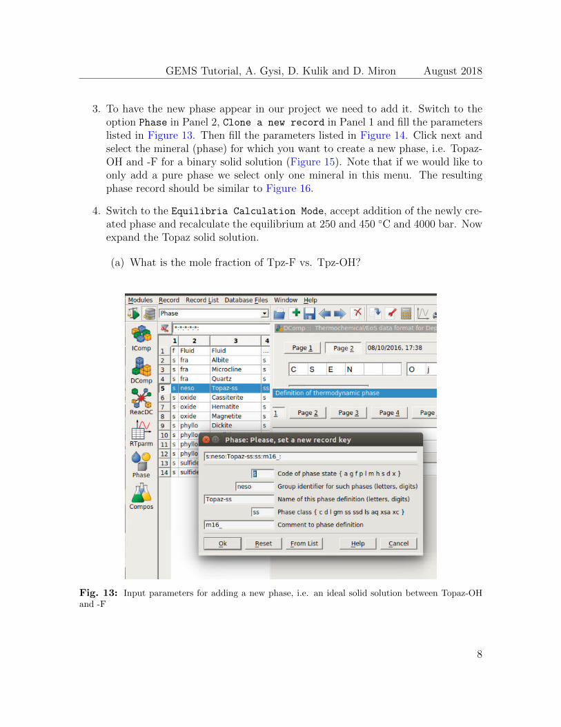
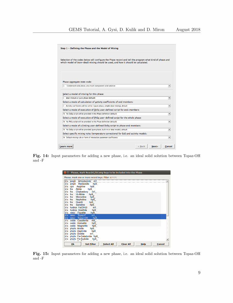
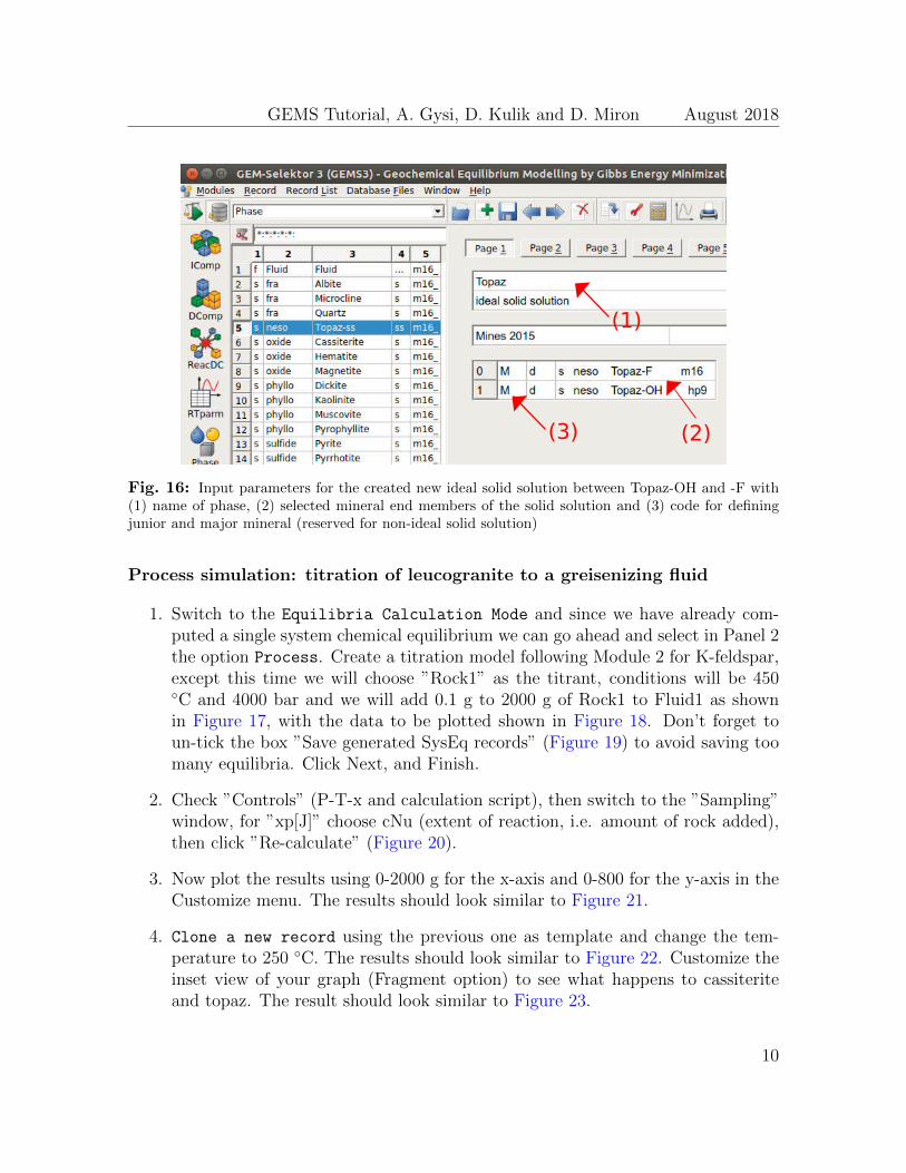
3. To have the new phase appear in our project we need to add it. Switch to theoption Phase in Panel 2, Clone a new record in Panel 1 and fill the parameterslisted in Figure 13. Then fill the parameters listed in Figure 14. Click next andselect the mineral (phase) for which you want to create a new phase, i.e. Topaz-OH and -F for a binary solid solution (Figure 15). Note that if we would like toonly add a pure phase we select only one mineral in this menu. The resultingphase record should be similar to Figure 16.

4. Switch to the Equilibria Calculation Mode, accept addition of the newly cre-ated phase and recalculate the equilibrium at 250 and 450 ◦C and 4000 bar. Nowexpand the Topaz solid solution.

(a) What is the mole fraction of Tpz-F vs. Tpz-OH?

Fig. 13: Input parameters for adding a new phase, i.e. an ideal solid solution between Topaz-OHand -F

8




9


(1)

(2)(3)

Fig. 16: Input parameters for the created new ideal solid solution between Topaz-OH and -F with(1) name of phase, (2) selected mineral end members of the solid solution and (3) code for definingjunior and major mineral (reserved for non-ideal solid solution)

Process simulation: titration of leucogranite to a greisenizing fluid

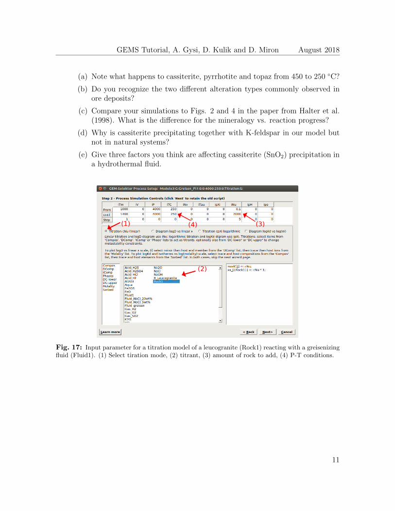
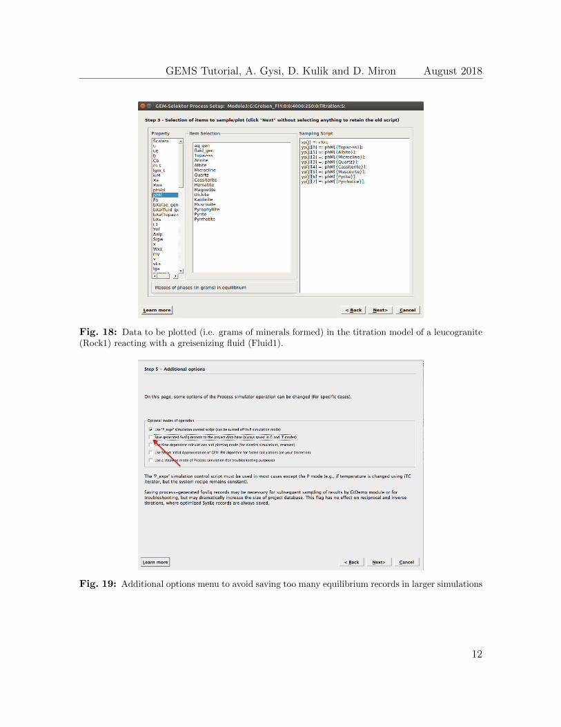
1. Switch to the Equilibria Calculation Mode and since we have already com-puted a single system chemical equilibrium we can go ahead and select in Panel 2the option Process. Create a titration model following Module 2 for K-feldspar,except this time we will choose ”Rock1” as the titrant, conditions will be 450◦C and 4000 bar and we will add 0.1 g to 2000 g of Rock1 to Fluid1 as shownin Figure 17, with the data to be plotted shown in Figure 18. Don’t forget toun-tick the box ”Save generated SysEq records” (Figure 19) to avoid saving toomany equilibria. Click Next, and Finish.

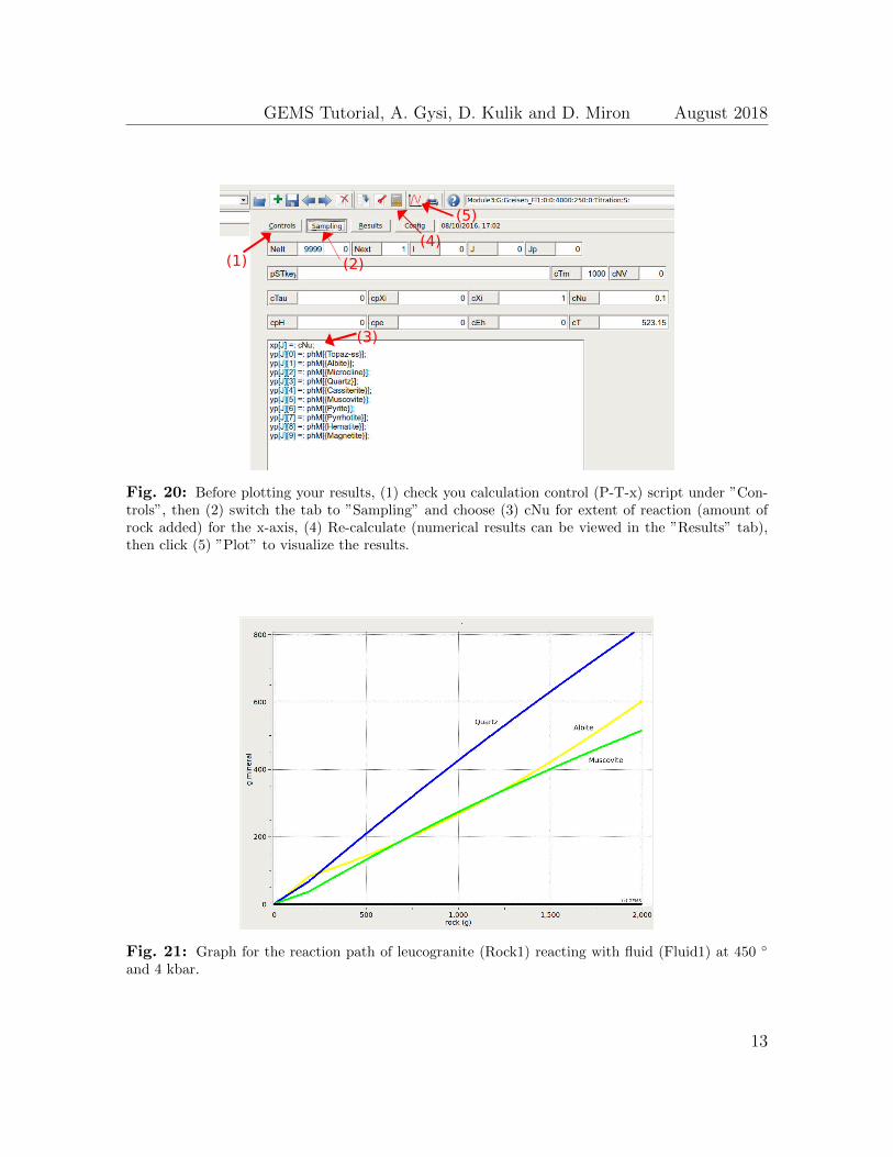
2. Check ”Controls” (P-T-x and calculation script), then switch to the ”Sampling”window, for ”xp[J]” choose cNu (extent of reaction, i.e. amount of rock added),then click ”Re-calculate” (Figure 20).

3. Now plot the results using 0-2000 g for the x-axis and 0-800 for the y-axis in theCustomize menu. The results should look similar to Figure 21.

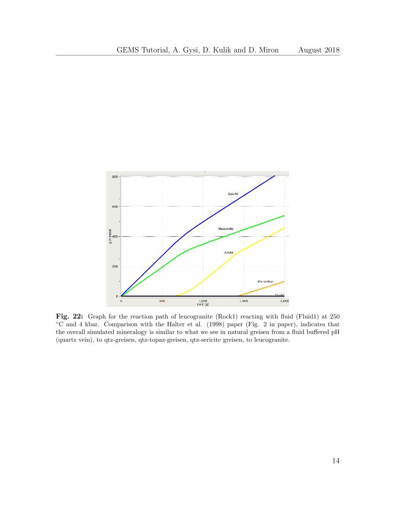
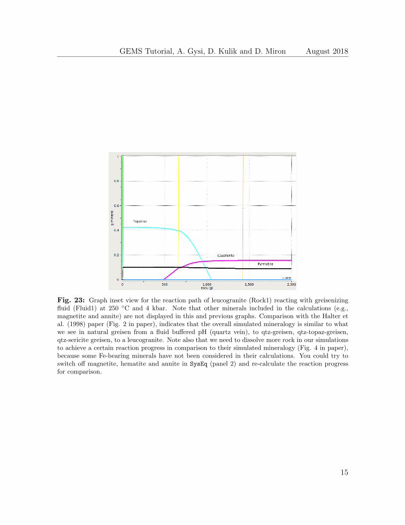
4. Clone a new record using the previous one as template and change the tem-perature to 250 ◦C. The results should look similar to Figure 22. Customize theinset view of your graph (Fragment option) to see what happens to cassiteriteand topaz. The result should look similar to Figure 23.

10


(a) Note what happens to cassiterite, pyrrhotite and topaz from 450 to 250 ◦C?

(b) Do you recognize the two different alteration types commonly observed inore deposits?

(c) Compare your simulations to Figs. 2 and 4 in the paper from Halter et al.(1998). What is the difference for the mineralogy vs. reaction progress?

(d) Why is cassiterite precipitating together with K-feldspar in our model butnot in natural systems?

(e) Give three factors you think are affecting cassiterite (SnO2) precipitation ina hydrothermal fluid.

(3)(1)

(2)

(4)

Fig. 17: Input parameter for a titration model of a leucogranite (Rock1) reacting with a greisenizingfluid (Fluid1). (1) Select tiration mode, (2) titrant, (3) amount of rock to add, (4) P-T conditions.

11


Fig. 18: Data to be plotted (i.e. grams of minerals formed) in the titration model of a leucogranite(Rock1) reacting with a greisenizing fluid (Fluid1).

Fig. 19: Additional options menu to avoid saving too many equilibrium records in larger simulations

12


(3)

(1) (2)

(4)

(5)

Fig. 20: Before plotting your results, (1) check you calculation control (P-T-x) script under ”Con-trols”, then (2) switch the tab to ”Sampling” and choose (3) cNu for extent of reaction (amount ofrock added) for the x-axis, (4) Re-calculate (numerical results can be viewed in the ”Results” tab),then click (5) ”Plot” to visualize the results.

Fig. 21: Graph for the reaction path of leucogranite (Rock1) reacting with fluid (Fluid1) at 450 ◦

and 4 kbar.

13


Fig. 22: Graph for the reaction path of leucogranite (Rock1) reacting with fluid (Fluid1) at 250◦C and 4 kbar. Comparison with the Halter et al. (1998) paper (Fig. 2 in paper), indicates thatthe overall simulated mineralogy is similar to what we see in natural greisen from a fluid buffered pH(quartz vein), to qtz-greisen, qtz-topaz-greisen, qtz-sericite greisen, to leucogranite.

14


Fig. 23: Graph inset view for the reaction path of leucogranite (Rock1) reacting with greisenizingfluid (Fluid1) at 250 ◦C and 4 kbar. Note that other minerals included in the calculations (e.g.,magnetite and annite) are not displayed in this and previous graphs. Comparison with the Halter etal. (1998) paper (Fig. 2 in paper), indicates that the overall simulated mineralogy is similar to whatwe see in natural greisen from a fluid buffered pH (quartz vein), to qtz-greisen, qtz-topaz-greisen,qtz-sericite greisen, to a leucogranite. Note also that we need to dissolve more rock in our simulationsto achieve a certain reaction progress in comparison to their simulated mineralogy (Fig. 4 in paper),because some Fe-bearing minerals have not been considered in their calculations. You could try toswitch off magnetite, hematite and annite in SysEq (panel 2) and re-calculate the reaction progressfor comparison.

15

Documents

MODULE 3: GREISEN ALTERATION (PART I)tdb.mines.edu/Tutorials/Module3.pdfMODULE 3: GREISEN ALTERATION (PART I) In this tutorial we will use the GEMS project le "Module3" in the examples