Embed Size (px)
Citation preview
NPTEL – Mechanical – Principle of Fluid Dynamics
Joint initiative of IITs and IISc – Funded by MHRD Page 1 of 56
Module 3 : Lecture 1 INVISCID INCOMPRESSIBLE FLOW
(Fundamental Aspects)
In general, fluids have a well-known tendency to move or flow. The slight change in
shear stress or appropriate imbalance in normal stresses will cause fluid motion. Fluid
kinematics deals with various aspects of fluid motion without concerning the actual
force that causes the fluid motion. In this particular section, we shall consider the
‘field’ concept to define velocity/ acceleration of fluid by virtue of its motion. In the
later part, some ‘visualization’ concepts are introduced to define the motion of the
fluid qualitatively as well as quantitatively.
There are two general approaches in analyzing the fluid motion. In the first
method (Lagrangian approach), the individual fluid particles are considered and their
properties are studied as a function of time. In the second method (Eulerian
approach), the ‘field’ concept is introduced and the properties are completely
prescribed as the functions of space and time. In other words, the attention is focused
at fixed points in space as the fluid passes those points.
Velocity and Acceleration Field
Since the ‘continuum’ assumption holds well for fluids, the description of any fluid
property (such as density, pressure, velocity, acceleration etc.) can be expressed as a
function of location. These representation as a function of spatial coordinates is called
as “field representation” of the flow. One of the most important fluid variables is the
velocity field. It is a vector function of position and time with components , andu v w
as scalar variables i.e.
( ) ( ) ( ) ˆˆ ˆ, , , , , , , , ,V u x y z t i v x y z t j w x y z t k= + +
(3.1.1)
The magnitude of the velocity vector i.e. ( )2 2 2V u v w= + +
, is the speed of fluid.
The total time derivative of the velocity vector is the acceleration vector field ( )a of
the flow which is given as,
( ){ } ( ){ } ( ){ }, , , , , , , , , ˆˆ ˆd u x y z t d v x y z t d w x y z tdVa i j kdt dt dt dt
= = + +
(3.1.2)
NPTEL – Mechanical – Principle of Fluid Dynamics
Joint initiative of IITs and IISc – Funded by MHRD Page 2 of 56
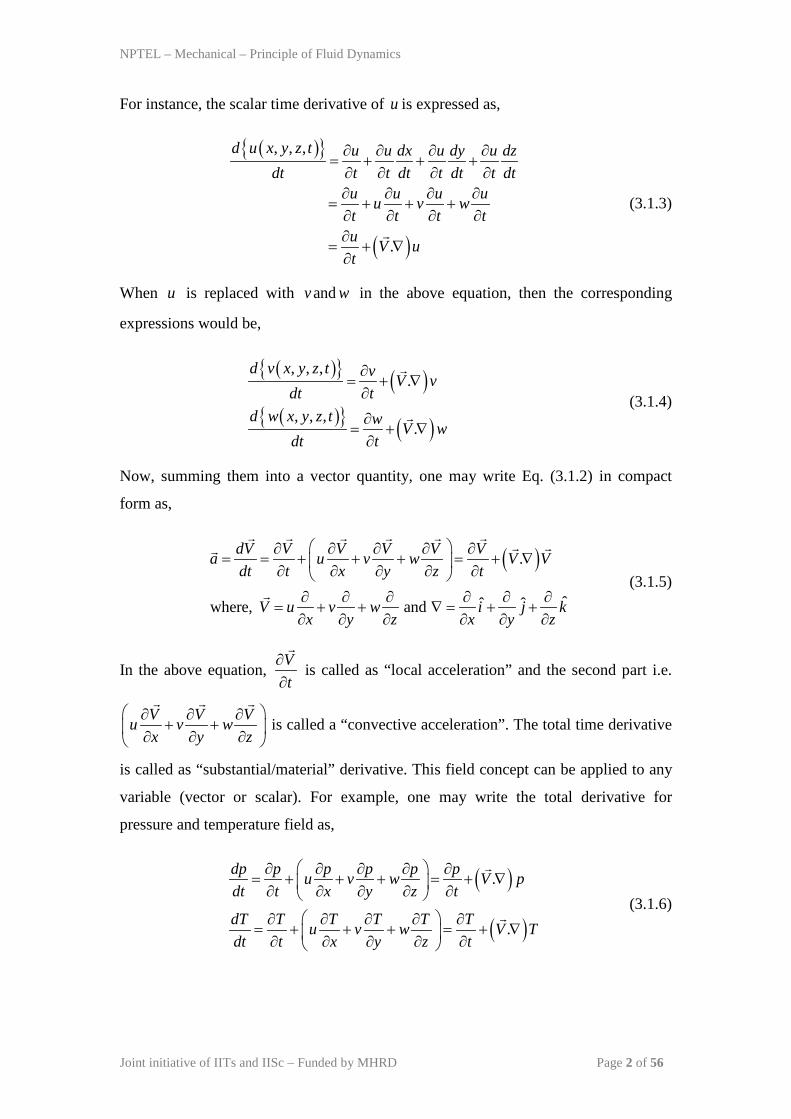
For instance, the scalar time derivative of u is expressed as,
( ){ }
( )
, , ,
.
d u x y z t u u dx u dy u dzdt t t dt t dt t dt
u u u uu v wt t t tu V ut
∂ ∂ ∂ ∂= + + +∂ ∂ ∂ ∂∂ ∂ ∂ ∂
= + + +∂ ∂ ∂ ∂∂
= + ∇∂
(3.1.3)
When u is replaced with andv w in the above equation, then the corresponding
expressions would be,
( ){ } ( )( ){ } ( )
, , ,.
, , ,.
d v x y z t v V vdt t
d w x y z t w V wdt t
∂= + ∇∂
∂= + ∇∂
(3.1.4)
Now, summing them into a vector quantity, one may write Eq. (3.1.2) in compact
form as,
( ).
ˆˆ ˆwhere, and
dV V V V V Va u v w V Vdt t x y z t
V u v w i j kx y z x y z
∂ ∂ ∂ ∂ ∂= = + + + = + ∇ ∂ ∂ ∂ ∂ ∂
∂ ∂ ∂ ∂ ∂ ∂= + + ∇ = + +
∂ ∂ ∂ ∂ ∂ ∂
(3.1.5)
In the above equation, Vt
∂∂
is called as “local acceleration” and the second part i.e.
V V Vu v wx y z
∂ ∂ ∂+ + ∂ ∂ ∂
is called a “convective acceleration”. The total time derivative
is called as “substantial/material” derivative. This field concept can be applied to any
variable (vector or scalar). For example, one may write the total derivative for
pressure and temperature field as,
( )
( )
.
.
dp p p p p pu v w V pdt t x y z t
dT T T T T Tu v w V Tdt t x y z t
∂ ∂ ∂ ∂ ∂= + + + = + ∇ ∂ ∂ ∂ ∂ ∂
∂ ∂ ∂ ∂ ∂= + + + = + ∇ ∂ ∂ ∂ ∂ ∂
(3.1.6)
NPTEL – Mechanical – Principle of Fluid Dynamics
Joint initiative of IITs and IISc – Funded by MHRD Page 3 of 56
Visualization of Fluid Flow
The quantitative and qualitative information of fluid flow can be obtained through
sketches, photographs, graphical representation and mathematical analysis. However,
the visual representation of flow fields is very important in modeling the flow
phenomena. In general, there are four basic types of line patterns used to visualize the
flow such as timeline, pathline, streakline and streamlines. Regardless of how the
results are obtained, (i.e. analytically/experimentally/computationally) it is necessary
to plot the data to get the feel of flow parameters that vary in time and/or shape (such
as profile plots, vector plots and contour plots).
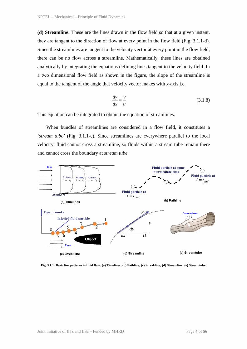
(a) Timeline: A ‘timeline’ is a set of fluid particles that form a line at a given instant
(Fig. 3.1.1-a). Thus, it is marked at same instant of time. Subsequent observations of
the line provide the information of the flow field. They are particularly useful in
situations where uniformity of flow is to be examined.
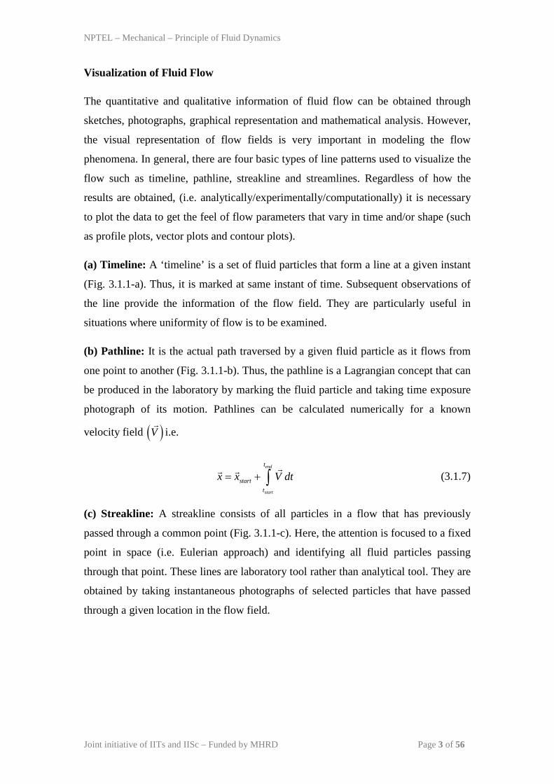
(b) Pathline: It is the actual path traversed by a given fluid particle as it flows from
one point to another (Fig. 3.1.1-b). Thus, the pathline is a Lagrangian concept that can
be produced in the laboratory by marking the fluid particle and taking time exposure
photograph of its motion. Pathlines can be calculated numerically for a known
velocity field ( )V
i.e.
end
start
t
startt
x x V dt= + ∫ (3.1.7)
(c) Streakline: A streakline consists of all particles in a flow that has previously
passed through a common point (Fig. 3.1.1-c). Here, the attention is focused to a fixed
point in space (i.e. Eulerian approach) and identifying all fluid particles passing
through that point. These lines are laboratory tool rather than analytical tool. They are
obtained by taking instantaneous photographs of selected particles that have passed
through a given location in the flow field.
NPTEL – Mechanical – Principle of Fluid Dynamics
Joint initiative of IITs and IISc – Funded by MHRD Page 4 of 56
(d) Streamline: These are the lines drawn in the flow field so that at a given instant,
they are tangent to the direction of flow at every point in the flow field (Fig. 3.1.1-d).
Since the streamlines are tangent to the velocity vector at every point in the flow field,
there can be no flow across a streamline. Mathematically, these lines are obtained
analytically by integrating the equations defining lines tangent to the velocity field. In
a two dimensional flow field as shown in the figure, the slope of the streamline is
equal to the tangent of the angle that velocity vector makes with x-axis i.e.
dy vdx u
= (3.1.8)
This equation can be integrated to obtain the equation of streamlines.
When bundles of streamlines are considered in a flow field, it constitutes a
‘stream tube’ (Fig. 3.1.1-e). Since streamlines are everywhere parallel to the local
velocity, fluid cannot cross a streamline, so fluids within a stream tube remain there
and cannot cross the boundary at stream tube.
Fig. 3.1.1: Basic line patterns in fluid flow: (a) Timelines; (b) Pathline; (c) Streakline; (d) Streamline; (e) Streamtube.
NPTEL – Mechanical – Principle of Fluid Dynamics
Joint initiative of IITs and IISc – Funded by MHRD Page 5 of 56
The following observations can be made about the fundamental line patterns;
1. Mathematically, it is convenient to calculate a streamline while other three are
easier to generate experimentally.
2. The streamlines and timelines are instantaneous lines while pathlines and
streakline are generated by passage of time.
3. In a steady flow, all the four basic line patterns are identical. Since, the
velocity at each point in the flow field remains constant with time,
consequently streamline shapes do not vary. It implies that the particle located
on a given streamline will always move along the same streamline. Further,
the consecutive particles passing through a fixed point in space will be on the
same streamline. Hence, all the lines are identical in a steady flow. They do
not coincide for unsteady flows.
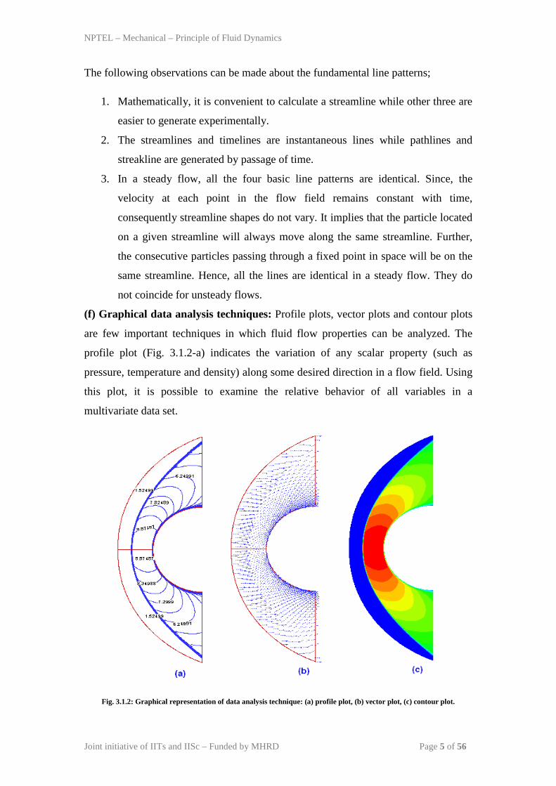
(f) Graphical data analysis techniques: Profile plots, vector plots and contour plots
are few important techniques in which fluid flow properties can be analyzed. The
profile plot (Fig. 3.1.2-a) indicates the variation of any scalar property (such as
pressure, temperature and density) along some desired direction in a flow field. Using
this plot, it is possible to examine the relative behavior of all variables in a
multivariate data set.
Fig. 3.1.2: Graphical representation of data analysis technique: (a) profile plot, (b) vector plot, (c) contour plot.
NPTEL – Mechanical – Principle of Fluid Dynamics
Joint initiative of IITs and IISc – Funded by MHRD Page 6 of 56
A vector plot (Fig. 3.1.2-b) is an array of arrows indicating the magnitude and
direction of a vector property at an instant of time. Although, streamlines indicate the
direction of instantaneous velocity field, but does not directly indicate the magnitude
of velocity. A useful flow pattern for both experimental and computational fluid flow
is the ‘vector plot’ that indicates the magnitude and direction of instantaneous vector
property.
A contour plot (Fig. 3.1.2-c) is a two-dimensional plot of a three-dimensional
surface showing lines where the surface intersects planes of constant elevation. Thus,
they are curves with constant values of scalar property (or magnitude of vector
property) at an instant of time. They can be filled in with either colors or sheds of gray
representing the magnitude of the property.
NPTEL – Mechanical – Principle of Fluid Dynamics
Joint initiative of IITs and IISc – Funded by MHRD Page 7 of 56
Module 3 : Lecture 2 INVISCID INCOMPRESSIBLE FLOW (Kinematic Description of Fluid Flow)
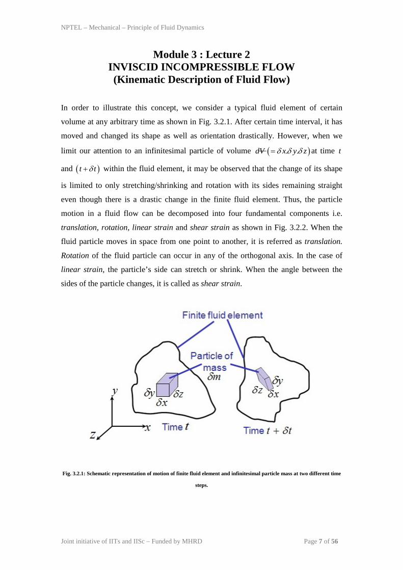
In order to illustrate this concept, we consider a typical fluid element of certain
volume at any arbitrary time as shown in Fig. 3.2.1. After certain time interval, it has
moved and changed its shape as well as orientation drastically. However, when we
limit our attention to an infinitesimal particle of volume ( ). .dV x y zδ δ δ= at time t
and ( )t tδ+ within the fluid element, it may be observed that the change of its shape
is limited to only stretching/shrinking and rotation with its sides remaining straight
even though there is a drastic change in the finite fluid element. Thus, the particle
motion in a fluid flow can be decomposed into four fundamental components i.e.
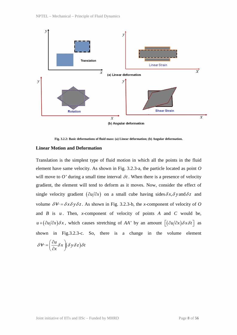
translation, rotation, linear strain and shear strain as shown in Fig. 3.2.2. When the
fluid particle moves in space from one point to another, it is referred as translation.
Rotation of the fluid particle can occur in any of the orthogonal axis. In the case of
linear strain, the particle’s side can stretch or shrink. When the angle between the
sides of the particle changes, it is called as shear strain.
Fig. 3.2.1: Schematic representation of motion of finite fluid element and infinitesimal particle mass at two different time
steps.
NPTEL – Mechanical – Principle of Fluid Dynamics
Joint initiative of IITs and IISc – Funded by MHRD Page 8 of 56
Fig. 3.2.2: Basic deformations of fluid mass: (a) Linear deformation; (b) Angular deformation.
Linear Motion and Deformation
Translation is the simplest type of fluid motion in which all the points in the fluid
element have same velocity. As shown in Fig. 3.2.3-a, the particle located as point O
will move to O’ during a small time interval tδ . When there is a presence of velocity
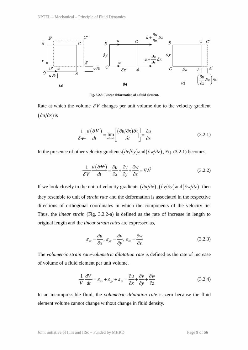
gradient, the element will tend to deform as it moves. Now, consider the effect of
single velocity gradient ( )u x∂ ∂ on a small cube having sides , andx y zδ δ δ and
volume V x y zδ δ δ δ= . As shown in Fig. 3.2.3-b, the x-component of velocity of O
and B is u . Then, x-component of velocity of points A and C would be,
( )u u x xδ+ ∂ ∂ , which causes stretching of AA’ by an amount ( )u x x tδ δ∂ ∂ as
shown in Fig.3.2.3-c. So, there is a change in the volume element
( )uV x y z tx
δ δ δ δ δ∂ = ∂
NPTEL – Mechanical – Principle of Fluid Dynamics
Joint initiative of IITs and IISc – Funded by MHRD Page 9 of 56
Fig. 3.2.3: Linear deformation of a fluid element.
Rate at which the volume Vδ changes per unit volume due to the velocity gradient
( )u x∂ ∂ is
( ) ( )0
1 limt
d V u x t uV dt t xδ
δ δδ δ→
∂ ∂ ∂= = ∂
(3.2.1)
In the presence of other velocity gradients ( ) ( )andv y w z∂ ∂ ∂ ∂ , Eq. (3.2.1) becomes,
( )1 .d V u v w V
V dt x y zδ
δ∂ ∂ ∂
= + + = ∇∂ ∂ ∂
(3.2.2)
If we look closely to the unit of velocity gradients ( ) ( ) ( ), andu x v y w z∂ ∂ ∂ ∂ ∂ ∂ , then
they resemble to unit of strain rate and the deformation is associated in the respective
directions of orthogonal coordinates in which the components of the velocity lie.
Thus, the linear strain (Fig. 3.2.2-a) is defined as the rate of increase in length to
original length and the linear strain rates are expressed as,
, ,xx yy zzu v wx y z
ε ε ε∂ ∂ ∂= = =∂ ∂ ∂
(3.2.3)
The volumetric strain rate/volumetric dilatation rate is defined as the rate of increase
of volume of a fluid element per unit volume.
1xx yy zz
dV u v wV dt x y z
ε ε ε ∂ ∂ ∂= + + = + +
∂ ∂ ∂ (3.2.4)
In an incompressible fluid, the volumetric dilatation rate is zero because the fluid
element volume cannot change without change in fluid density.
NPTEL – Mechanical – Principle of Fluid Dynamics
Joint initiative of IITs and IISc – Funded by MHRD Page 10 of 56
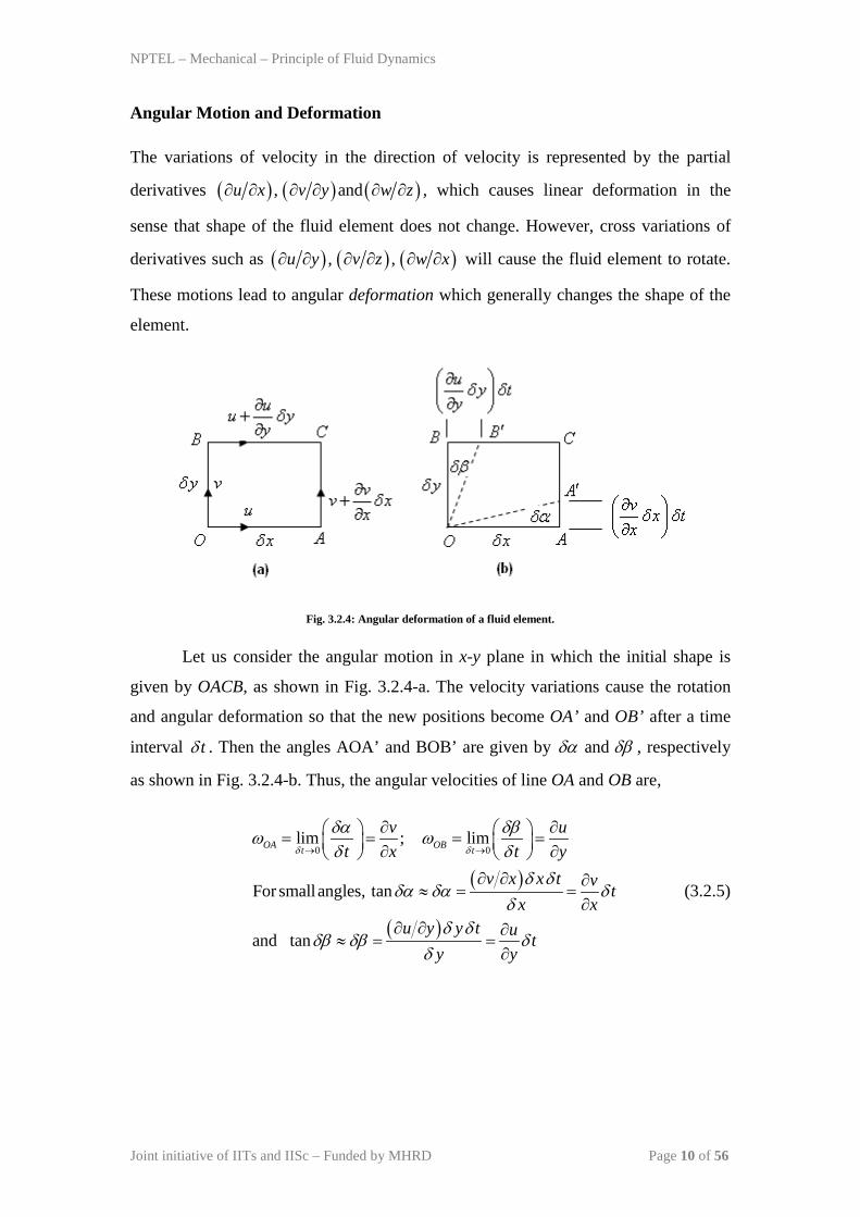
Angular Motion and Deformation
The variations of velocity in the direction of velocity is represented by the partial
derivatives ( ) ( ) ( ), andu x v y w z∂ ∂ ∂ ∂ ∂ ∂ , which causes linear deformation in the
sense that shape of the fluid element does not change. However, cross variations of
derivatives such as ( ) ( ) ( ), ,u y v z w x∂ ∂ ∂ ∂ ∂ ∂ will cause the fluid element to rotate.
These motions lead to angular deformation which generally changes the shape of the
element.
Fig. 3.2.4: Angular deformation of a fluid element.
Let us consider the angular motion in x-y plane in which the initial shape is
given by OACB, as shown in Fig. 3.2.4-a. The velocity variations cause the rotation
and angular deformation so that the new positions become OA’ and OB’ after a time
interval tδ . Then the angles AOA’ and BOB’ are given by andδα δβ , respectively
as shown in Fig. 3.2.4-b. Thus, the angular velocities of line OA and OB are,
( )
( )
0 0lim ; lim
For smallangles, tan
and tan
OA OBt t
v ut x t y
v x x t v tx x
u y y t u ty y
δ δ
δα δβω ωδ δ
δ δδα δα δ
δδ δ
δβ δβ δδ
→ →
∂ ∂ = = = = ∂ ∂ ∂ ∂ ∂
≈ = =∂
∂ ∂ ∂≈ = =
∂
(3.2.5)
NPTEL – Mechanical – Principle of Fluid Dynamics
Joint initiative of IITs and IISc – Funded by MHRD Page 11 of 56
When, both ( ) ( )andv x u y∂ ∂ ∂ ∂ are positive, then both andOA OBω ω
will be in
counterclockwise direction. Now, the rotation of the fluid element about z-direction
(i.e x-y plane) zω can be defined as the average of andOA OBω ω . If counterclockwise
rotation is considered as positive, then
12z
v ux y
ω ∂ ∂
= − ∂ ∂ (3.2.6)
In a similar manner, the rotation of the fluid element about x and y axes are denoted as
andx yω ω , respectively.
1 1;2 2x y
w v u wy z z x
ω ω ∂ ∂ ∂ ∂ = − = − ∂ ∂ ∂ ∂
(3.2.7)
These three components can be combined to define the rotation vector ( )ω in the form
as,
ˆˆ ˆ
1 1 1 ˆˆ ˆor,2 2 2
ˆˆ ˆ
1 1or,2 2
x y zi j k
w v u w v ui j ky z z x x y
i j k
Vx y z
u v w
ω ω ω ω
ω
ω
= + +
∂ ∂ ∂ ∂ ∂ ∂ = − + − + − ∂ ∂ ∂ ∂ ∂ ∂
∂ ∂ ∂= = ∇×
∂ ∂ ∂
(3.2.8)
It is observed from Eq.(3.2.6) that the fluid element will rotate about z-axis, as an
undeformed block, only when, ( ) ( )i.e.OA OB v x u yω ω= − ∂ ∂ = − ∂ ∂ . Otherwise it will
be associated with angular deformation which is characterized by shear strain rate.
When the fluid element undergoes shear deformation (Fig. 3.2.2-b), the average shear
strain rates expressed in different cartesian planes as,
1 1 1; ;2 2 2xy yz zx
v u w v w ux y y z z x
ε ε ε ∂ ∂ ∂ ∂ ∂ ∂ = + = + = + ∂ ∂ ∂ ∂ ∂ ∂
(3.2.9)
NPTEL – Mechanical – Principle of Fluid Dynamics
Joint initiative of IITs and IISc – Funded by MHRD Page 12 of 56
Strain rate as a whole constitute a symmetric second order tensor i.e.
xx xy xz
ij yx yy yz
zx zy zz
ε ε εε ε ε ε
ε ε ε
=
(3.2.10)
Vorticity
In a flow field, vorticity is related to fluid particle velocity which is defined as twice
of rotation vector i.e.
ˆˆ ˆ2 w v u w v uV i j ky z z x x y
ζ ω ∂ ∂ ∂ ∂ ∂ ∂ = = ∇× = − + − + − ∂ ∂ ∂ ∂ ∂ ∂
(3.2.11)
Thus, the curl of the velocity vector is equal to the vorticity. It leads to two important
definitions:
If 0V∇× ≠
at every point in the flow, the flow is called as rotational. It
implies that the fluid elements have a finite angular velocity.
If 0V∇× =
at every point in the flow, the flow is called as irrotational. It
implies that the fluid elements have no angular velocity rather the motion is
purely translational.
Irrotational Flow
In Eq.(3.2.11) , if 0V∇× =
is zero, then the rotation and vorticity are zero. The flow
fields for which the above condition is applicable is known as irrotational flow. The
condition of irrotationality imposes specific relationship among the velocity gradients
which is applicable for inviscid flow. If the rotations about the respective orthogonal
axes are to be zero, then, one can write Eq. (3.2.11) as,
0 ; 0 ; 0z y xv u u w w vx y z x y z
ω ω ω∂ ∂ ∂ ∂ ∂ ∂= ⇒ = = ⇒ = = ⇒ =
∂ ∂ ∂ ∂ ∂ ∂ (3.2.12)
NPTEL – Mechanical – Principle of Fluid Dynamics
Joint initiative of IITs and IISc – Funded by MHRD Page 13 of 56
A general flow field would never satisfy all the above conditions. However, a uniform
flow field defined in a fashion, for which (a constant); 0; 0u U v w= = = , is
certainly an example of an irrotational flow because there are no velocity gradients. A
fluid flow which is initially irrotational may become rotational if viscous effects
caused by solid boundaries, entropy gradients and density gradients become
significant.
Circulation
It is defined as the line integral of the tangential velocity component about any closed
curve fixed in the flow i.e.
.V dsΓ = ∫
(3.2.13)
where, ds is an elemental vector tangent to the curve and with length ds with
counterclockwise path of integration considered as positive. For the closed curve path
OACB as shown in Fig. 3.2.4-a, we can develop the relationship between circulation
and vorticity as follows;
( )
or, 2
Then, . 2
z
z zA A
v uu x v x y u y x v yx y
v u x y x yx y
V ds dA V dA
δ δ δ δ δ δ δ
δ δ δ ω δ δ
ω
∂ ∂ Γ = + + − + − ∂ ∂ ∂ ∂
Γ = − = ∂ ∂
Γ = = = ∇×∫ ∫ ∫
(3.2.14)
Hence, circulation around a closed contour is equal to total vorticity enclosed within
it. It is known as Stokes theorem in two dimensions.
NPTEL – Mechanical – Principle of Fluid Dynamics
Joint initiative of IITs and IISc – Funded by MHRD Page 14 of 56
Module 3 : Lecture 3 INVISCID INCOMPRESSIBLE FLOW (Stream Function and Velocity Potential)
Basic Equations of Fluid Motion
The differential relations for fluid particle can be written for conservation of mass,
momentum and energy. In addition, there are two state relations for thermodynamic
properties. They can be summarized as;
( )
( ) ( )
( ) ( )
Continuity: . 0
Momentum: .
Energy: . .
Thermodynamicstate relations: , ; ,
ij
Vt
dV g pdt
e p V k Tt
p T e e p T
ρ ρ
ρ ρ τ
ρ
ρ ρ
∂+∇ =
∂
= −∇ +∇
∂+ ∇ = ∇ ∇ +Φ
∂= =
(3.3.1)
Here, Φ is the viscous-dissipation function, e is the internal energy and k is the
thermal conductivity of the fluid. In general, the density is a variable and all these
equations have 5-unknown parameters i.e. , , , andV p e Tρ
. In an incompressible flow
with constant viscosity, the momentum equation can be decoupled from energy
equation. Thus, continuity and momentum equations are solved simultaneously for
pressure and velocity. However, there are certain flow situations, which can wipe out
continuity equation by defining a suitable variable (called as stream function) and
thereby solving the momentum equation with a single variable.
NPTEL – Mechanical – Principle of Fluid Dynamics
Joint initiative of IITs and IISc – Funded by MHRD Page 15 of 56
Stream Function
The idea of introducing stream function works only if the continuity equation is
reduced to two terms. There are 4-terms in the continuity equation that one can get by
expanding the vector equation (3.3.1) i.e.
( ) ( ) ( ) 0u v w
t x y zρ ρ ρρ ∂ ∂ ∂∂
+ + + =∂ ∂ ∂ ∂
(3.3.2)
For a steady, incompressible, plane, two-dimensional flow, this equation reduces to,
0u vx y∂ ∂
+ =∂ ∂
(3.3.3)
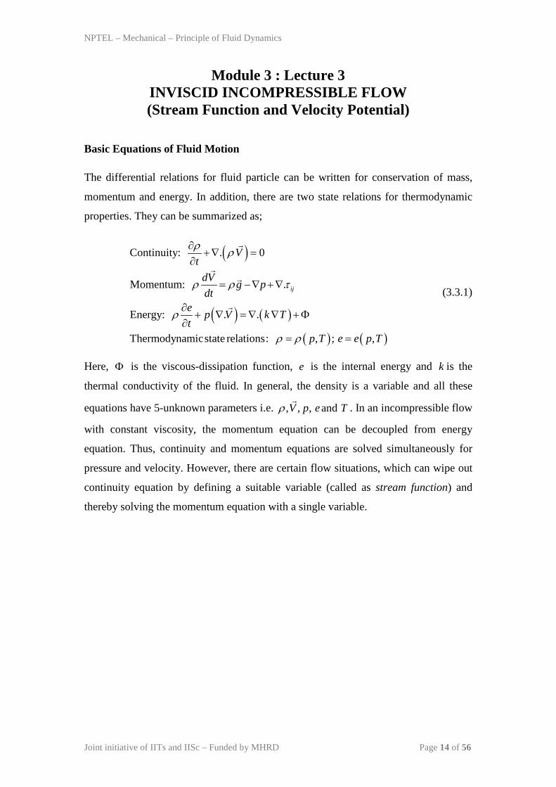
Here, the striking idea of stream function works that will eliminate two velocity
components andu v into a single variable (Fig. 3.3.1-a). So, the stream function
( ){ },x yψ relates to the velocity components in such a way that continuity equation
(3.3.3) is satisfied.
;
ˆ ˆor,
u vy x
V i jy x
ψ ψ
ψ ψ
∂ ∂= = −∂ ∂
∂ ∂= −∂ ∂
(3.3.4)
Fig. 3.3.1: Velocity components along a streamline.
NPTEL – Mechanical – Principle of Fluid Dynamics
Joint initiative of IITs and IISc – Funded by MHRD Page 16 of 56
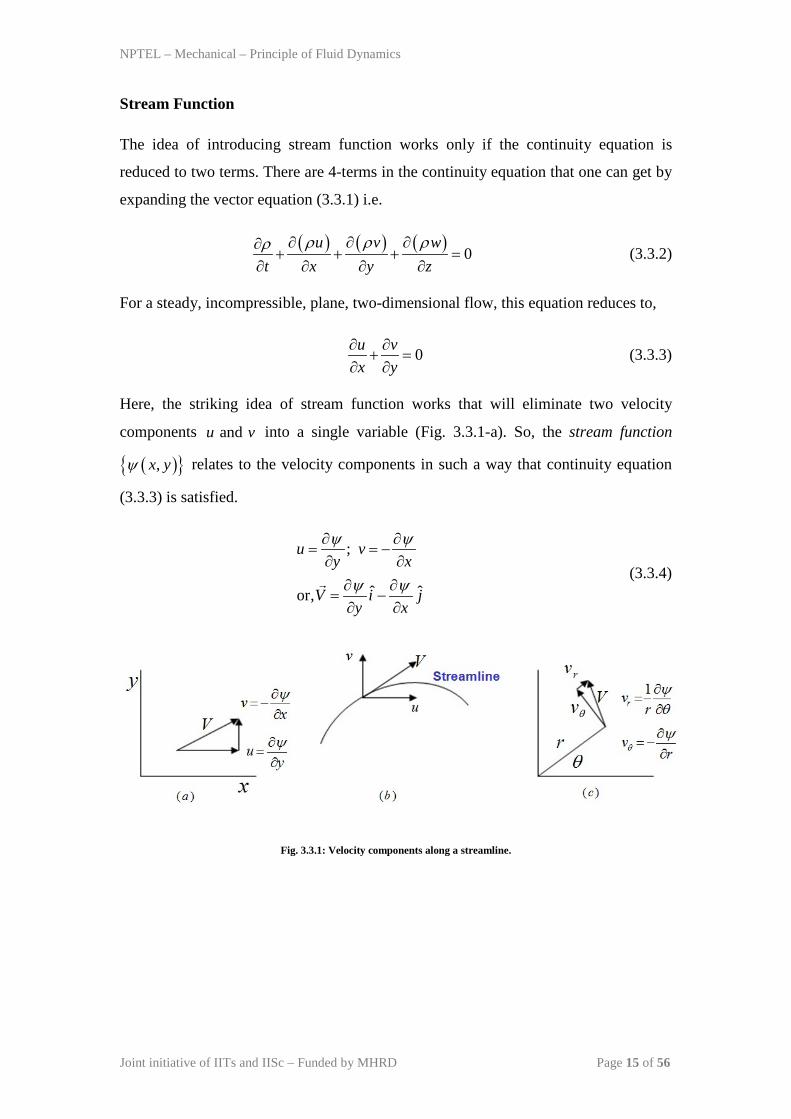
Fig. 3.3.2: Flow between two streamlines.
The following important points can be noted for stream functions;
1. The lines along which ψ is constant are called as streamlines. In a flow field, the
tangent drawn at every point along a streamline shows the direction of velocity (Fig.
3.3.1-b). So, the slope at any point along a streamline is given by,
dy vdx u
= (3.3.5)
Referring to the Fig. 3.3.2-a, if we move from one point ( ),x y to a nearby point
( ),x dx y dy+ + , then the corresponding change in the value of stream function is dψ
which is given by,
d dx dy v dx u dyx yψ ψψ ∂ ∂
= + = − +∂ ∂
(3.3.6)
Along a line of constant ψ ,
0
or,
d v dx u dydy vdx u
ψ = − + =
= (3.3.7)
The Eq. (3.3.5) is same as that of Eq. (3.3.7). Hence, it is the defining equation for the
streamline. Thus, infinite number streamlines can be drawn with constant ψ . This
family of streamlines will be useful in visualizing the flow patterns. It may also be
noted that streamlines are always parallel to each other.
NPTEL – Mechanical – Principle of Fluid Dynamics
Joint initiative of IITs and IISc – Funded by MHRD Page 17 of 56
2. The numerical constant associated toψ , represents the volume rate of flow.
Consider two closely spaced streamlines ( )and dψ ψ ψ+ as shown in Fig. 3.3.2-a.
Let dq represents the volume rate of flow per unit width perpendicular to x-y plane,
passing between the streamlines. At any arbitrary surface AC, this volume flow must
be equal to net outflow through surfaces AB and BC. Thus,
or,
dq v dx u dy dx dy dx y
dq d
ψ ψ ψ
ψ
∂ ∂= − + = + =
∂ ∂=
(3.3.8)
Hence, the volume flow rate ( )q can be determined by integrating Eq. (3.3.8) between
streamlines 1 2andψ ψ as follows;
2
1
2 1q dψ
ψ
ψ ψ ψ= = −∫ (3.3.9)
So, the change in the value of stream function is equal to volume rate of flow. If the
upper streamline 2ψ has a value greater than the lower one 1ψ , then the volume flow
rate is positive i.e. flow takes place from left to right (Fig. 3.3.2-b).
3. In cylindrical coordinates, the continuity equation for a steady, incompressible,
plane, two-dimensional flow, reduces to
( )1 1 0rr v vr r r
θ
θ∂ ∂
+ =∂ ∂
(3.3.10)
The respective velocity components andrv vθ are shown in Fig. 3.3.1-c. The stream
function ( ){ },rψ θ that satisfies Eq. (3.3.10), can then be defined as,
1 ;rv vr rθ
ψ ψθ
∂ ∂= = −
∂ ∂ (3.3.11)
NPTEL – Mechanical – Principle of Fluid Dynamics
Joint initiative of IITs and IISc – Funded by MHRD Page 18 of 56
4. In a steady, plane compressible flow, the stream function can be defined by
including the density of the fluid. But, the change in the stream function is equal to
mass flow rate ( )m .
;
or,
u vy x
dm v dx u dy dx dy dx y
dm d
ψ ψρ ρ
ψ ψρ ρ ψ
ψ
∂ ∂= = −∂ ∂
∂ ∂= − + = + =
∂ ∂=
(3.3.12)
5. One important application in a two-dimensional plane is the inviscid and
irroational flow where, there is no velocity gradient and 0zω = . Then, the vorticity
vector becomes,
2 2
2 2
2
ˆ ˆ2 0
ˆor, 0
or, 0
or, 0
zv uk kx y
kx x y y
x y
ζ ω
ψ ψ
ψ ψ
ψ
∂ ∂= = − = ∂ ∂ ∂ ∂ ∂ ∂ − − = ∂ ∂ ∂ ∂ ∂ ∂
− =∂ ∂
∇ =
(3.3.13)
This is a second order equation and is quite popular in mathematics and is known as
Laplace equation in a two-dimensional plane.
Velocity Potential
An irrotational flow is defined as the flow where the vorticity is zero at every point. It
gives rise to a scalar function ( )φ which is similar and complementary to the stream
function ( )ψ . Let us consider the equations of irrortional flow and scalar function ( )φ
. In an irrotational flow, there is no vorticity ( )ξ
0Vξ = ∇× =
(3.3.14)
Now, take the vector identity of the scalar function ( )φ ,
( ) 0φ∇× ∇ = (3.3.15)
NPTEL – Mechanical – Principle of Fluid Dynamics
Joint initiative of IITs and IISc – Funded by MHRD Page 19 of 56
i.e. a vector with zero curl must be the gradient of a scalar function or, curl of the
gradient of a scalar function is identically zero. Comparing, Eqs. (3.3.14) and (3.3.15),
we see that,
V φ= ∇
(3.3.16)
Here, φ is called as velocity potential function and its gradient gives rise to velocity
vector. The knowledge φ immediately gives the velocity components. In cartesian
coordinates, the velocity potential function can be defined as, ( ), ,x y zφ φ= so that
Eq. (3.3.16) can be written as,
ˆ ˆˆ ˆ ˆ ˆu i v j wk i j kx y zφ φ φ∂ ∂ ∂
+ + = + +∂ ∂ ∂
(3.3.17)
So, the velocity components can be written as,
; ;u v wx y zφ φ φ∂ ∂ ∂
= = =∂ ∂ ∂
(3.3.18)
In cylindrical coordinates, if ( ), ,r zφ φ θ= , then
; ;r zV V Vr zθφ φ φ
θ∂ ∂ ∂
= = =∂ ∂ ∂
(3.3.19)
Further, if the flow is incompressible i.e. ( )constant and 0tρ ρ= ∂ ∂ = , then
continuity equation can be written as,
( )( )
. 0
or, . 0
or, . 0
Vt
V
V
ρ ρ
ρ
∂+∇ =
∂
∇ =
∇ =
(3.3.20)
NPTEL – Mechanical – Principle of Fluid Dynamics
Joint initiative of IITs and IISc – Funded by MHRD Page 20 of 56
Therefore, for a flow which is incompressible and irrotational, Eqs. (3.3.16) and
(3.3.20) can be combined to yield a second order Laplace equation in a three-
dimensional plane.
( )2
2 2 2
2 2 2
. 0
or, 0
or, 0x y z
φ
φ
φ φ φ
∇ ∇ =
∇ =
∂ ∂ ∂+ + =
∂ ∂ ∂
(3.3.21)
Thus, any irrotational, incompressible flow has a velocity potential and stream
function (for two-dimensional flow) that both satisfy Laplace equation. Conversely,
any solution of Laplace equation represents both velocity potential and stream
function (two-dimensional) for an irrotational, incompressible flow.
An irrotational flow allows a velocity potential to be defined and leads to
simplification of fundamental equations. Instead of dealing with the velocity
components , andu v w as unknowns, one can deal with only one parameterφ , for a
given problem. Since, the irrotational flows are best described by velocity potential,
such flows are called as potential flows. In these flows, the lines with constant φ , is
known as equipotential lines. In addition, a line drawn in space such that φ∇ is the
tangent at every point is defined as a gradient line and thus can be called as
streamline.
Stream Function vs Velocity Potential
The velocity potential is analogous to stream function in a sense that the derivatives of
both andφ ψ yield the flow field velocities. However, there are distinct differences
between andφ ψ :
The flow field velocities are obtained by differentiating φ in the same
direction as the velocities, whereas, ψ is differentiated normal to the velocity
direction.
The velocity potential is defined for irrotational flows only. In contrast, stream
function can be used in either rotational or irrotational flows.
The velocity potential applies to three-dimensional flows, whereas the stream
function is defined for two dimensional flows only.
NPTEL – Mechanical – Principle of Fluid Dynamics
Joint initiative of IITs and IISc – Funded by MHRD Page 21 of 56
It is seen that the stream lines are defined as lines of constant ψ which are same
as gradient lines and perpendicular to lines of constant φ . So, the equipotential lines
and stream lines are mutually perpendicular. In order to illustrate the results more
clearly, let us consider a two-dimensional, irrotational, incompressible flow in
Cartesian coordinates.
For a streamline, ( ), constantx yψ = , and the differential of ψ is zero.
constant
0
or, 0
or,
d dx dyx y
d v dx u dydy vdx uψ
ψ ψψ
ψ
=
∂ ∂= + =∂ ∂= − + =
=
(3.3.22)
Similarly, for an equipotential line, ( ), constantx yφ = , and the differential of φ is
zero.
constant
0
or, 0
or,
d dx dyx y
d u dx v dydy udx vφ
φ φφ
φ
=
∂ ∂= + =∂ ∂= + =
= −
(3.3.23)
Combining Eqs. (3.3.22) and (3.3.23), we can write,
( )constant constant
1dydx dy dxψ φ= =
= −
(3.3.24)
Hence, the streamlines and equipotential lines are mutually perpendicular.
NPTEL – Mechanical – Principle of Fluid Dynamics
Joint initiative of IITs and IISc – Funded by MHRD Page 22 of 56
Module 3 : Lecture 4 INVISCID INCOMPRESSIBLE FLOW
(Basic Potential Flows - I)
Potential Theory
In a plane irrotaional flow, one can use either velocity potential or stream function to
define the flow field and both must satisfy Laplace equation. Moreover, the analysis
of this equation is much easier than direct approach of fully viscous Navier-Stokes
equations. Since the Laplace equation is linear, various solutions can be added to
obtain other solutions. Thus, if we have certain basic solutions, then they can be
combined to obtain complicated and interesting solutions. The analysis of such flow
field solutions of Laplace equation is termed as potential theory. The potential theory
has a lot of practical implications defining complicated flows. Here, we shall discuss
the stream function and velocity potential for few elementary flow fields such as
uniform flow, source/sink flow and vortex flow. Subsequently, they can be
superimposed to obtain complicated flow fields of practical relevance.
Governing equations for irrotational and incompressible flow
The analysis of potential flow is dealt with combination of potential lines and
streamlines. In a planner flow, the velocities of the flow field can be defined in terms
of stream functions ( ){ },x yψ and potential functions ( ){ },x yφ as,
( ){ } ( ){ }
( ){ } ( ){ }
, ,;
, ,;
x y x yu v
y xx y x y
u vx y
ψ ψ
φ φ
∂ ∂= = −
∂ ∂
∂ ∂= =
∂ ∂
(3.4.1)
The stream function ψ is defined such that continuity equation is satisfied whereas,
for low speed irrotational flows ( )0V∇× =
, if the viscous effects are neglected, the
continuity equation ( )0V•∇ =
, reduces to Laplace equation for φ . Both the functions
satisfy the Laplace equations i.e.
2 2 2 2
2 2 2 20; 0x y x yφ φ ψ ψ∂ ∂ ∂ ∂+ = + =
∂ ∂ ∂ ∂ (3.4.2)
NPTEL – Mechanical – Principle of Fluid Dynamics
Joint initiative of IITs and IISc – Funded by MHRD Page 23 of 56
Thus, the following obvious and important conclusions can be drawn from Eq.
(3.4.2);
• Any irrotational, incompressible and planner flow (two-dimensional) has a
velocity potential and stream function and both the functions satisfy Laplace
equation.
• Conversely, any solution of Laplace equation represents the velocity potential
or stream function for an irrotational, incompressible and two-dimensional
flow.
Note that Eq. (3.4.2) is a second-order linear partial differential equation. If there are
n separate solutions such as, ( ) ( ) ( )1 2, , , ,........, ,nx y x y x yφ φ φ then the sum (Eq. 3.4.3)
is also a solution of Eq. (3.4.2).
( ) ( ) ( ) ( )1 2, , , ........ ,nx y x y x y x yφ φ φ φ= + + + (3.4.3)
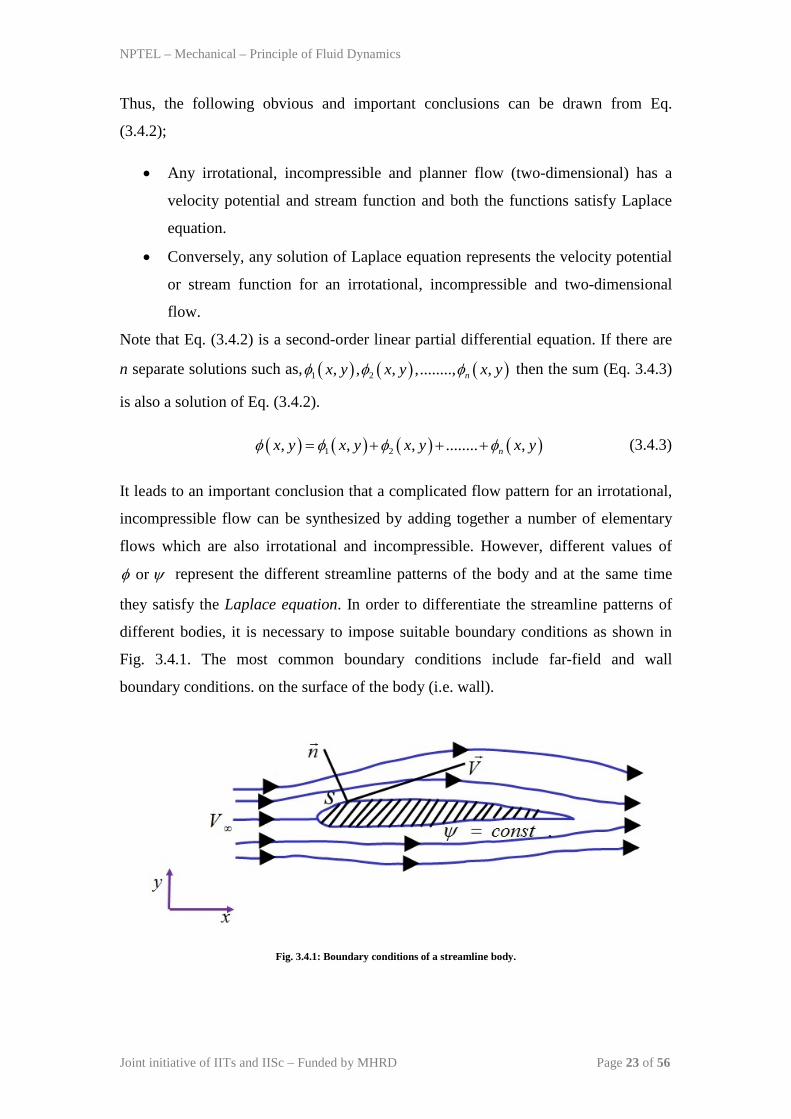
It leads to an important conclusion that a complicated flow pattern for an irrotational,
incompressible flow can be synthesized by adding together a number of elementary
flows which are also irrotational and incompressible. However, different values of
orφ ψ represent the different streamline patterns of the body and at the same time
they satisfy the Laplace equation. In order to differentiate the streamline patterns of
different bodies, it is necessary to impose suitable boundary conditions as shown in
Fig. 3.4.1. The most common boundary conditions include far-field and wall
boundary conditions. on the surface of the body (i.e. wall).
Fig. 3.4.1: Boundary conditions of a streamline body.
NPTEL – Mechanical – Principle of Fluid Dynamics
Joint initiative of IITs and IISc – Funded by MHRD Page 24 of 56
Far away from the body, the flow approaches uniform free stream conditions in
all directions. The velocity field is then specified in terms of stream function and
potential function as,
0
u Vy x
vx y
ψ φ
ψ φ
∞
∂ ∂= = =∂ ∂∂ ∂
= − = =∂ ∂
(3.4.4)
On the solid surface, there is no velocity normal to the body surface while the tangent
at any point on the surface defines the surface velocity. So, the boundary conditions
can be written in terms of stream and potential functions as,
0; 0n sφ ψ∂ ∂= =
∂ ∂ (3.4.5)
Here, s is the distance measured along the body surface and n is perpendicular to the
body. Thus, any line of constant ψ in the flow may be interpreted as body shape for
which there is no velocity normal to the surface. If the shape of the body is given by
( )by f x= , then =constantbbody y yψ ψ == is alternate boundary condition of Eq. (3.4.5).
If we deal with wall boundary conditions in terms of andu v , then the equation of
streamline evaluated at body surface is given by,
( )constant constant
1b
surfaceb
dy vdx dy dx uψ φ= =
= − =
(3.4.6)
It is seen that lines of constant φ (equi-potential lines) are orthogonal to lines of
constant ψ (streamlines) at all points where they intersect. Thus, for a potential flow
field, a flow-net consisting of family of streamlines and potential lines can be drawn,
which are orthogonal to each other. Both the set of lines are laplacian and they are
useful tools to visualize the flow field graphically.
NPTEL – Mechanical – Principle of Fluid Dynamics
Joint initiative of IITs and IISc – Funded by MHRD Page 25 of 56
Referring to the above discussion, the general approach to the solution of
irrotational, incompressible flows can be summarized as follows;
• Solve the Laplace equation for orφ ψ along with proper boundary
conditions.
• Obtain the flow velocity from Eq. (3.4.1)
• Obtain the pressure on the surface of the body using Bernoulli’s equation.
2 21 12 2
p V p Vρ ρ ∞∞+ = + (3.4.7)
In the subsequent section, the above solution procedure will be applied to some basic
elementary incompressible flows and later they will be superimposed to synthesize
more complex flow problems.
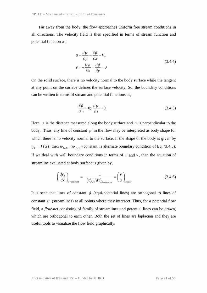
Uniform Flow
The simplest type of elementary flow for which the streamlines are straight, parallel
with constant velocity, is known as uniform flow. Consider a uniform flow in positive
x-direction as shown in Fig. 3.4.2. This flow can be represented as,
; 0u V v∞= = (3.4.8)
Fig. 3.4.2: Schematic representation of a uniform flow.
NPTEL – Mechanical – Principle of Fluid Dynamics
Joint initiative of IITs and IISc – Funded by MHRD Page 26 of 56
The uniform flow is a physically possible incompressible flow that satisfies continuity
equation ( )0V•∇ =
and the flow is irrotational ( )0V∇× =
. Hence, the velocity
potential can be written as,
; 0
; 0
u V vx y
u V vy y
φ φ
ψ ψ
∞
∞
∂ ∂= = = =
∂ ∂∂ ∂
= = = − =∂ ∂
(3.4.9)
Integrating Eq.(3.4.9) with respect to x,
( ) ( )( ) ( )
( ) ( )( ) ( )
1 1 1
1 1 1
1
2 2 2
2 2 2
2
;
and
;
and
V x f y g x C
g x V x f y CV x C
V y f x g y C
g y V y f x CV y C
φ φ
φψ ψ
ψ
∞
∞
∞
∞
∞
∞
= + = +
⇒ = =
⇒ = +
= + = +
⇒ = =
⇒ = +
(3.4.10)
In practical flow problems, the actual values of andφ ψ are not important, rather it is
always used as differentiation to obtain the velocity vector. Hence, the constant
appearing in Eq. (3.4.10) can be set to zero. Thus, for a uniform flow, the stream
functions and potential function can be written as,
;V x V yφ ψ∞ ∞= = (3.4.11)
NPTEL – Mechanical – Principle of Fluid Dynamics
Joint initiative of IITs and IISc – Funded by MHRD Page 27 of 56
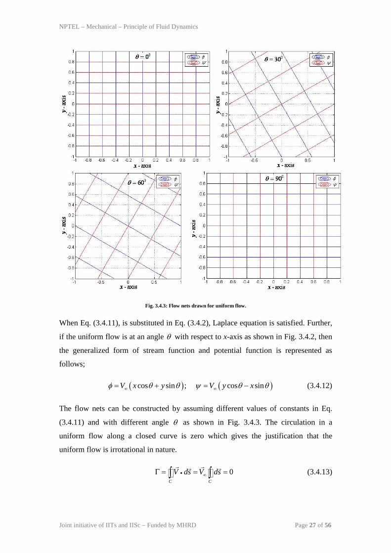
Fig. 3.4.3: Flow nets drawn for uniform flow.
When Eq. (3.4.11), is substituted in Eq. (3.4.2), Laplace equation is satisfied. Further,
if the uniform flow is at an angle θ with respect to x-axis as shown in Fig. 3.4.2, then
the generalized form of stream function and potential function is represented as
follows;
( ) ( )cos sin ; cos sinV x y V y xφ θ θ ψ θ θ∞ ∞= + = − (3.4.12)
The flow nets can be constructed by assuming different values of constants in Eq.
(3.4.11) and with different angle θ as shown in Fig. 3.4.3. The circulation in a
uniform flow along a closed curve is zero which gives the justification that the
uniform flow is irrotational in nature.
0C C
V ds V ds• ∞Γ = = =∫ ∫
(3.4.13)
NPTEL – Mechanical – Principle of Fluid Dynamics
Joint initiative of IITs and IISc – Funded by MHRD Page 28 of 56
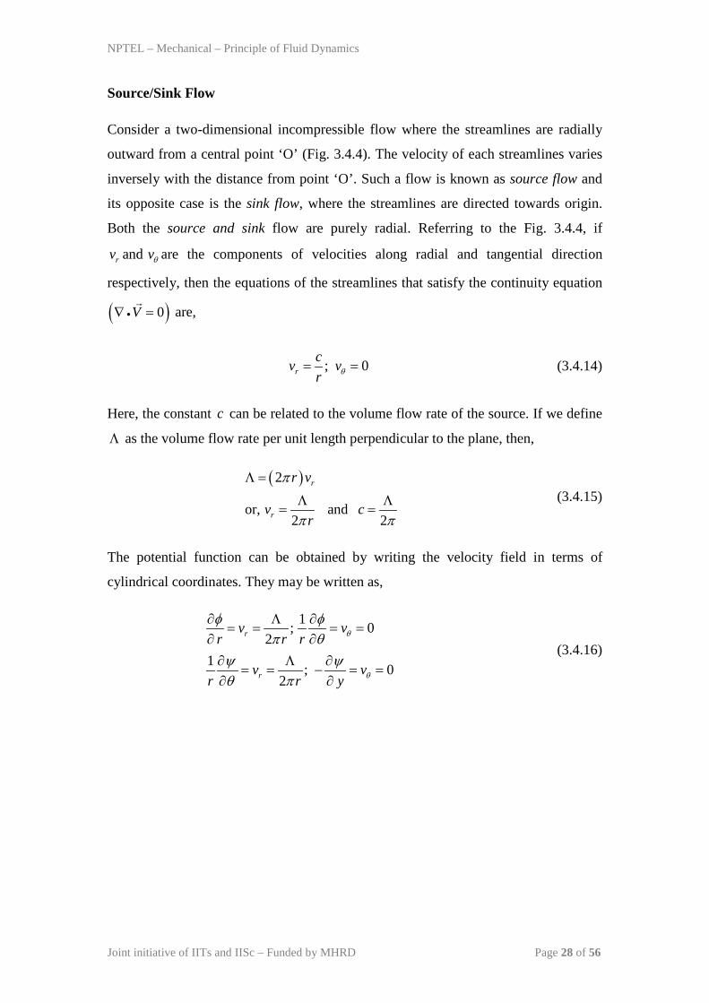
Source/Sink Flow
Consider a two-dimensional incompressible flow where the streamlines are radially
outward from a central point ‘O’ (Fig. 3.4.4). The velocity of each streamlines varies
inversely with the distance from point ‘O’. Such a flow is known as source flow and
its opposite case is the sink flow, where the streamlines are directed towards origin.
Both the source and sink flow are purely radial. Referring to the Fig. 3.4.4, if
andrv vθ are the components of velocities along radial and tangential direction
respectively, then the equations of the streamlines that satisfy the continuity equation
( )0V•∇ =
are,
; 0rcv vr θ= = (3.4.14)
Here, the constant c can be related to the volume flow rate of the source. If we define
Λ as the volume flow rate per unit length perpendicular to the plane, then,
( )2
or, and2 2
r
r
r v
v cr
π
π π
Λ =
Λ Λ= =
(3.4.15)
The potential function can be obtained by writing the velocity field in terms of
cylindrical coordinates. They may be written as,
1; 02
1 ; 02
r
r
v vr r r
v vr r y
θ
θ
φ φπ θ
ψ ψθ π
∂ Λ ∂= = = =
∂ ∂∂ Λ ∂
= = − = =∂ ∂
(3.4.16)
NPTEL – Mechanical – Principle of Fluid Dynamics
Joint initiative of IITs and IISc – Funded by MHRD Page 29 of 56
Fig. 3.4.4: Schematic representation of a source and sink flow.
Integrating Eq. (3.4.16) with respect to andr θ , we can get the equation for potential
function and stream function for a source and sink flow.
( ) ( )
( ) ( )
( ) ( )
( ) ( )
3 3 3
3 3 3
3
4 4 4
4 4 4
4
ln ;2
and ln2
ln2
;2
and2
2
r f C g r
f C g r r
r C
f r C g
f r C g
C
φ θ φπ
θπ
φπ
ψ θ ψ θπ
θπ
ψ θπ
Λ= + = +
Λ⇒ = =
Λ⇒ = +
Λ= + = +
Λ⇒ = =
Λ⇒ = +
(3.4.17)
The constant appearing in Eqs (3.4.17) can be dropped to obtain the stream function
and potential function.
ln ;2 2
rφ ψ θπ πΛ Λ
= = (3.4.18)
This equation will also satisfy the Laplace equation in the polar coordinates. Also, it
represents the streamlines to be straight and radially outward/inward depending on the
source or sink flow while the potential lines are concentric circles shown as flow nets
in Fig. 3.4.5. Both the streamlines and equi-potential lines are mutually perpendicular.
NPTEL – Mechanical – Principle of Fluid Dynamics
Joint initiative of IITs and IISc – Funded by MHRD Page 30 of 56
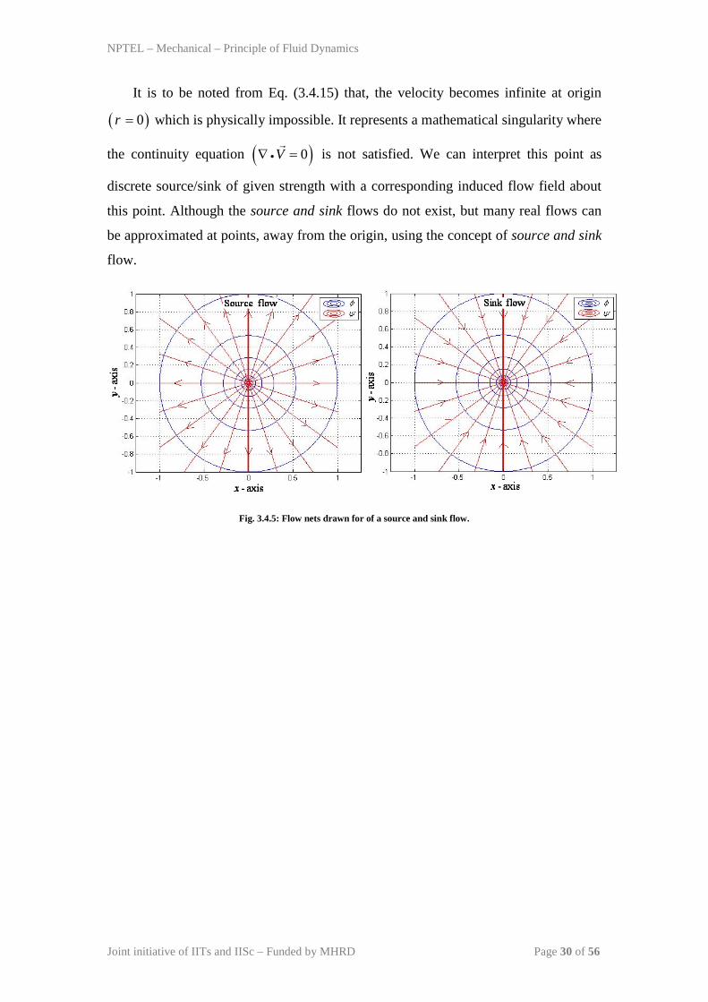
It is to be noted from Eq. (3.4.15) that, the velocity becomes infinite at origin
( )0r = which is physically impossible. It represents a mathematical singularity where
the continuity equation ( )0V•∇ =
is not satisfied. We can interpret this point as
discrete source/sink of given strength with a corresponding induced flow field about
this point. Although the source and sink flows do not exist, but many real flows can
be approximated at points, away from the origin, using the concept of source and sink
flow.
Fig. 3.4.5: Flow nets drawn for of a source and sink flow.
NPTEL – Mechanical – Principle of Fluid Dynamics
Joint initiative of IITs and IISc – Funded by MHRD Page 31 of 56
Module 3 : Lecture 5 INVISCID INCOMPRESSIBLE FLOW
(Basic Potential Flows - II)
Doublet Flow
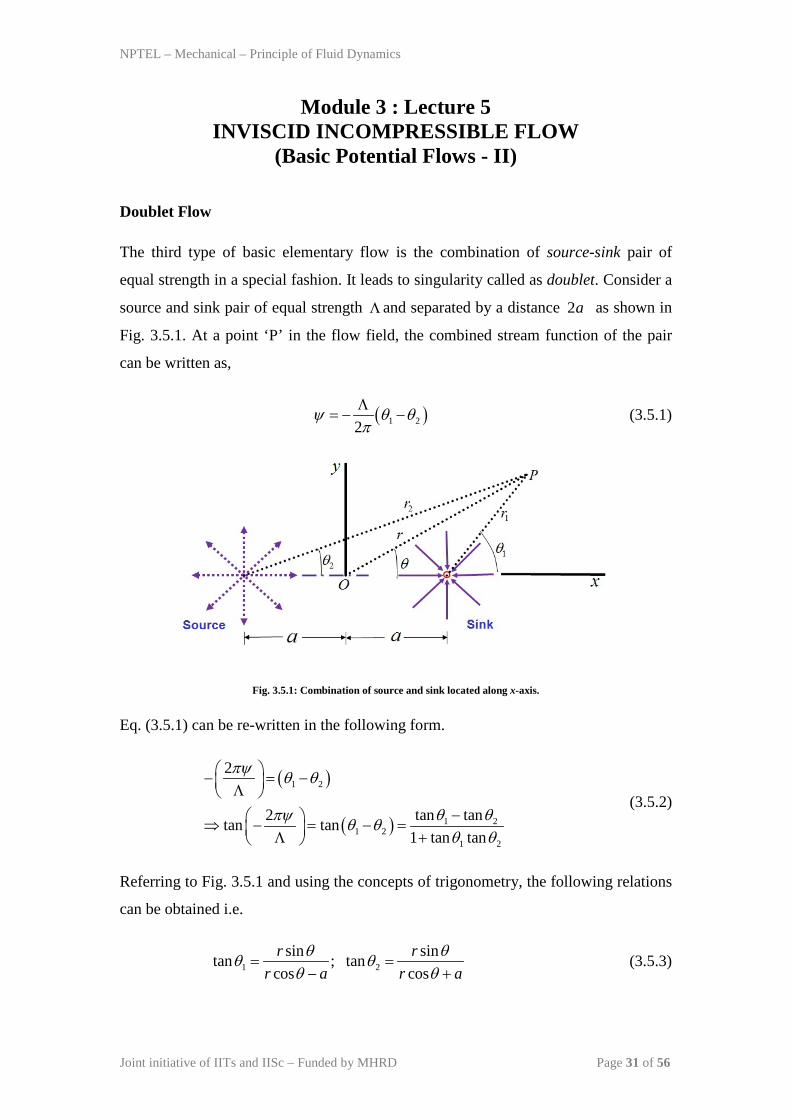
The third type of basic elementary flow is the combination of source-sink pair of
equal strength in a special fashion. It leads to singularity called as doublet. Consider a
source and sink pair of equal strength Λ and separated by a distance 2a as shown in
Fig. 3.5.1. At a point ‘P’ in the flow field, the combined stream function of the pair
can be written as,
( )1 22ψ θ θ
πΛ
= − − (3.5.1)
Fig. 3.5.1: Combination of source and sink located along x-axis.
Eq. (3.5.1) can be re-written in the following form.
( )
( )
1 2
1 21 2
1 2
2
tan tan2tan tan1 tan tan
πψ θ θ
θ θπψ θ θθ θ
− = − Λ − ⇒ − = − = Λ +
(3.5.2)
Referring to Fig. 3.5.1 and using the concepts of trigonometry, the following relations
can be obtained i.e.
1 2sin sintan ; tan
cos cosr r
r a r aθ θθ θ
θ θ= =
− + (3.5.3)
NPTEL – Mechanical – Principle of Fluid Dynamics
Joint initiative of IITs and IISc – Funded by MHRD Page 32 of 56
Substituting these results in Eq. (3.5.2), we can obtain,
( ) ( )
2 2
12 2
2 2
2 2 sintan
2 sintan2
sin For small values of
arr a
arr a
a r ar a
πψ θ
θψπ
θψπ
−
− = Λ − Λ ⇒ = − − Λ
⇒ = −−
(3.5.4)
Now, a doublet can be formed by bringing the source-sink pair as close to each other
( )0a → while increasing its strength ( )Λ →∞ and keeping the product ( )a πΛ
constant. Then, ( )2 2 1r r a r− → and Eq. (3.5.4) can be simplified as,
sinr
κ θψ = − (3.5.5)
Here, ( )2aκ π= Λ is a constant and called as strength of the doublet. Since the
stream function and potential function is mutually perpendicular, we can write the
velocity potential for the doublet as,
cosr
κ θφ = (3.5.6)
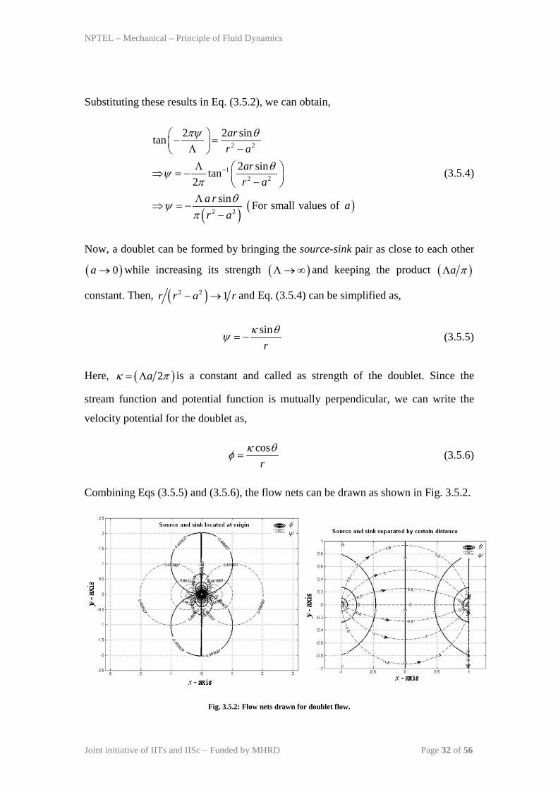
Combining Eqs (3.5.5) and (3.5.6), the flow nets can be drawn as shown in Fig. 3.5.2.
Fig. 3.5.2: Flow nets drawn for doublet flow.
NPTEL – Mechanical – Principle of Fluid Dynamics
Joint initiative of IITs and IISc – Funded by MHRD Page 33 of 56
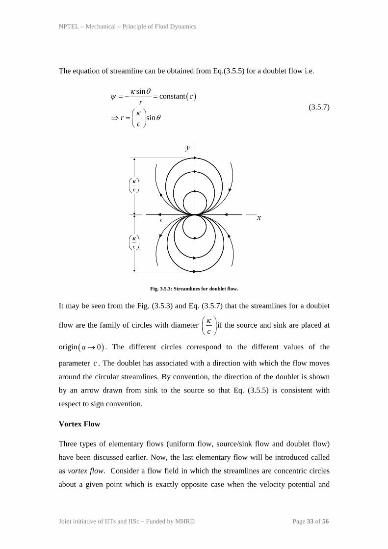
The equation of streamline can be obtained from Eq.(3.5.5) for a doublet flow i.e.
( )sin constant
sin
cr
rc
κ θψ
κ θ
= − =
⇒ =
(3.5.7)
Fig. 3.5.3: Streamlines for doublet flow.
It may be seen from the Fig. (3.5.3) and Eq. (3.5.7) that the streamlines for a doublet
flow are the family of circles with diameter cκ
if the source and sink are placed at
origin ( )0a → . The different circles correspond to the different values of the
parameter c . The doublet has associated with a direction with which the flow moves
around the circular streamlines. By convention, the direction of the doublet is shown
by an arrow drawn from sink to the source so that Eq. (3.5.5) is consistent with
respect to sign convention.
Vortex Flow
Three types of elementary flows (uniform flow, source/sink flow and doublet flow)
have been discussed earlier. Now, the last elementary flow will be introduced called
as vortex flow. Consider a flow field in which the streamlines are concentric circles
about a given point which is exactly opposite case when the velocity potential and
NPTEL – Mechanical – Principle of Fluid Dynamics
Joint initiative of IITs and IISc – Funded by MHRD Page 34 of 56
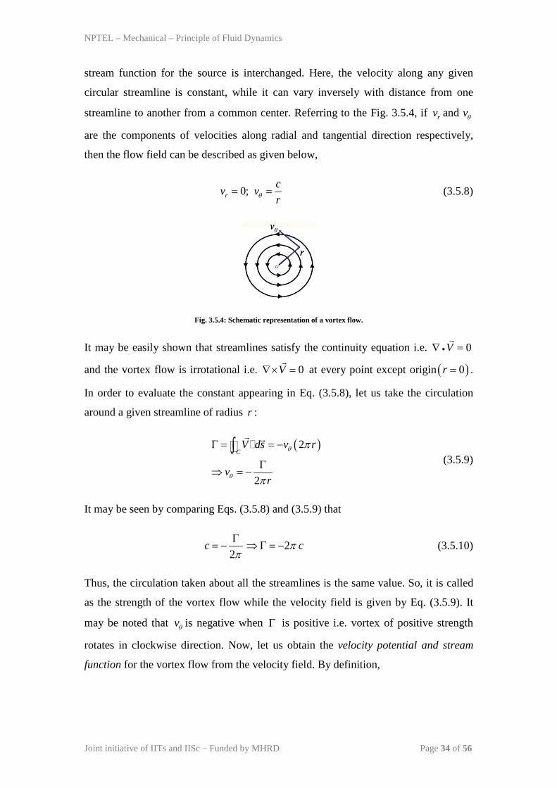
stream function for the source is interchanged. Here, the velocity along any given
circular streamline is constant, while it can vary inversely with distance from one
streamline to another from a common center. Referring to the Fig. 3.5.4, if andrv vθ
are the components of velocities along radial and tangential direction respectively,
then the flow field can be described as given below,
0;rcv vrθ= = (3.5.8)
Fig. 3.5.4: Schematic representation of a vortex flow.
It may be easily shown that streamlines satisfy the continuity equation i.e. 0V•∇ =
and the vortex flow is irrotational i.e. 0V∇× =
at every point except origin ( )0r = .
In order to evaluate the constant appearing in Eq. (3.5.8), let us take the circulation
around a given streamline of radius r :
( )2
2
CV ds v r
vr
θ
θ
π
π
Γ = = −
Γ⇒ = −
∫
(3.5.9)
It may be seen by comparing Eqs. (3.5.8) and (3.5.9) that
22
c cππΓ
= − ⇒ Γ = − (3.5.10)
Thus, the circulation taken about all the streamlines is the same value. So, it is called
as the strength of the vortex flow while the velocity field is given by Eq. (3.5.9). It
may be noted that vθ is negative when Γ is positive i.e. vortex of positive strength
rotates in clockwise direction. Now, let us obtain the velocity potential and stream
function for the vortex flow from the velocity field. By definition,
NPTEL – Mechanical – Principle of Fluid Dynamics
Joint initiative of IITs and IISc – Funded by MHRD Page 35 of 56
10;2
1 0;2
r
r
v vr r r
v vr r r
θ
θ
φ φθ π
ψ ψθ π
∂ ∂ Γ= = = = −
∂ ∂∂ ∂ Γ
= = − = = −∂ ∂
(3.5.11)
Integrating the above equations, the velocity potential and stream function are
obtained as,
; ln2 2
rφ θ ψπ πΓ Γ
= − = (3.5.12)
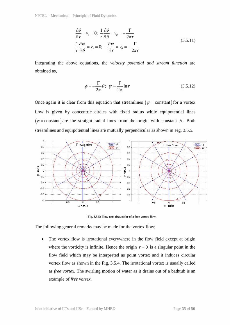
Once again it is clear from this equation that streamlines ( )constantψ = for a vortex
flow is given by concentric circles with fixed radius while equipotential lines
( )constantφ = are the straight radial lines from the origin with constant θ . Both
streamlines and equipotential lines are mutually perpendicular as shown in Fig. 3.5.5.
Fig. 3.5.5: Flow nets drawn for of a free vortex flow.
The following general remarks may be made for the vortex flow;
• The vortex flow is irrotational everywhere in the flow field except at origin
where the vorticity is infinite. Hence the origin 0r = is a singular point in the
flow field which may be interpreted as point vortex and it induces circular
vortex flow as shown in the Fig. 3.5.4. The irrotational vortex is usually called
as free vortex. The swirling motion of water as it drains out of a bathtub is an
example of free vortex.
NPTEL – Mechanical – Principle of Fluid Dynamics
Joint initiative of IITs and IISc – Funded by MHRD Page 36 of 56
• When the fluid particles rotate as a rigid body such that
1 1; is a constantv c r cθ = , then the vortex motion is rotational and it cannot be
described with velocity potential. This type of rotational vortex is commonly
called as forced vortex. The motion of a liquid contained in a tank, when
rotated about its axis with angular velocity ω corresponds to a forced vortex.
• A combined vortex is the one with a forced vortex as the central core and
velocity distribution corresponding to that of free vortex outside the core.
( ) ( )20 0;r
cv r r v r r rr θ ω= > = ≤ (3.5.13)
Here, 2 andc ω are constants and 0r is corresponds to the radius of the central
core.
NPTEL – Mechanical – Principle of Fluid Dynamics
Joint initiative of IITs and IISc – Funded by MHRD Page 37 of 56
Module 3 : Lecture 6 INVISCID INCOMPRESSIBLE FLOW
(Superposition of Potential Flows - I)
Method of Superposition
The potential flows are governed by the linear partial differential equation commonly
called as “Laplace Equation”. The elementary basic plane potential flows include
uniform flow, source/sink flow, doublet flow and free vortex flow. The details of
these flow fields have already been discussed and are summarized in the following
Table 3.6.1. A variety of interesting potential flow can be obtained by combination of
velocity potential and stream function of basic potential flows.
In an inviscid flow field, a streamline can be considered as a solid
boundary because there is no flow through it. Moreover, the conditions along the sold
boundary and the streamline are the same. Hence, the combinations of velocity
potential and stream functions of elementary flows will lead to a particular body
shape that can be interpreted as flow around that body. The method of solving such
potential flew problems is commonly called as, method of superposition.
NPTEL – Mechanical – Principle of Fluid Dynamics
Joint initiative of IITs and IISc – Funded by MHRD Page 38 of 56
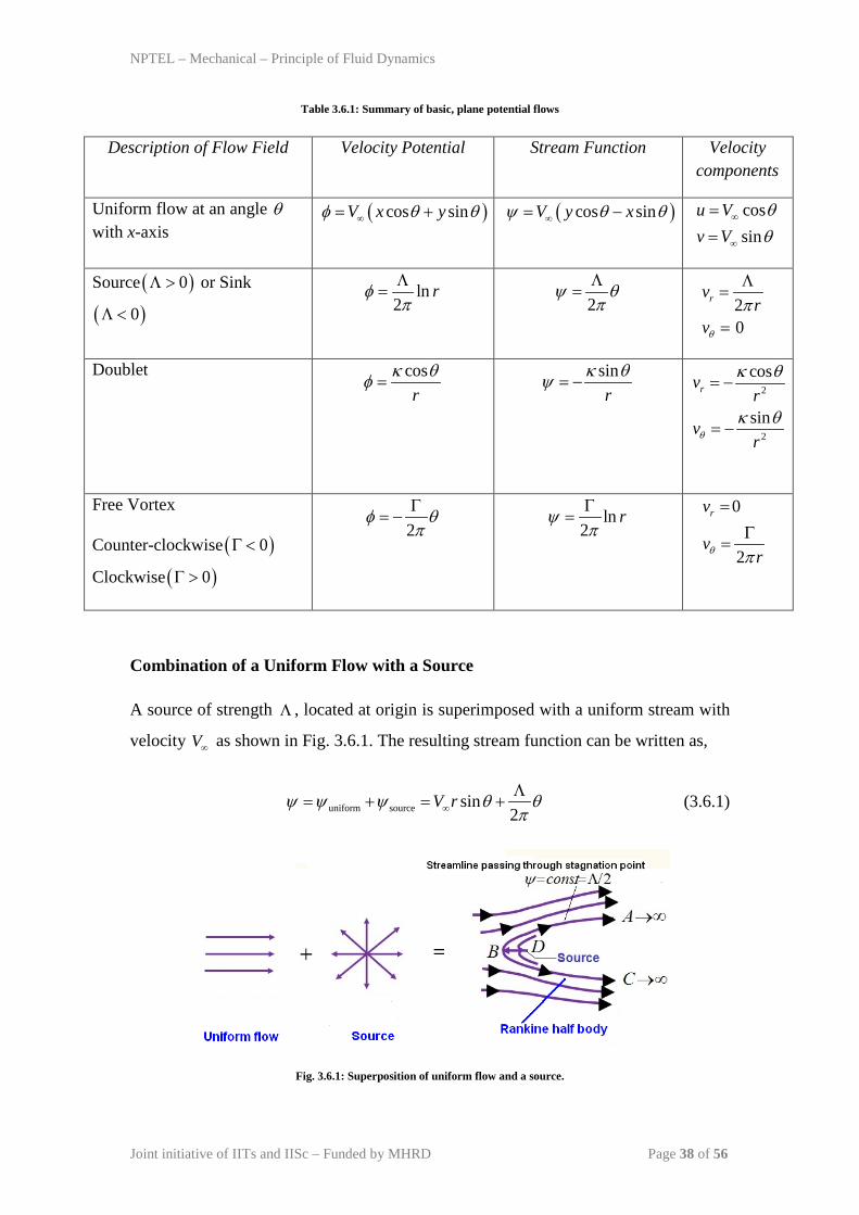
Table 3.6.1: Summary of basic, plane potential flows
Description of Flow Field Velocity Potential Stream Function Velocity components
Uniform flow at an angle θ with x-axis
( )cos sinV x yφ θ θ∞= +
( )cos sinV y xψ θ θ∞= −
cossin
u Vv V
θθ
∞
∞
==
Source ( )0Λ > or Sink
( )0Λ < ln
2rφ
πΛ
= 2
ψ θπΛ
= 20
rvr
vθπΛ
=
=
Doublet cosr
κ θφ =
sinr
κ θψ = −
2
2
cos
sin
rvr
vrθ
κ θ
κ θ
= −
= −
Free Vortex
Counter-clockwise ( )0Γ <
Clockwise ( )0Γ >
2φ θ
πΓ
= − ln2
rψπΓ
= 0
2
rv
vrθ π
=Γ
=
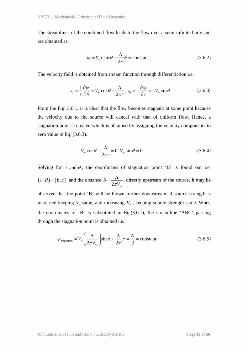
Combination of a Uniform Flow with a Source
A source of strength Λ , located at origin is superimposed with a uniform stream with
velocity V∞ as shown in Fig. 3.6.1. The resulting stream function can be written as,
uniform source sin2
V rψ ψ ψ θ θπ∞
Λ= + = + (3.6.1)
Fig. 3.6.1: Superposition of uniform flow and a source.
NPTEL – Mechanical – Principle of Fluid Dynamics
Joint initiative of IITs and IISc – Funded by MHRD Page 39 of 56
The streamlines of the combined flow leads to the flow over a semi-infinite body and
are obtained as,
sin constant2
V rψ θ θπ∞
Λ= + = (3.6.2)
The velocity field is obtained from stream function through differentiation i.e.
1 cos ; sin2rv V v V
r r rθψ ψθ θθ π∞ ∞
∂ Λ ∂= = + = − = −
∂ ∂ (3.6.3)
From the Fig. 3.6.1, it is clear that the flow becomes stagnant at some point because
the velocity due to the source will cancel with that of uniform flow. Hence, a
stagnation point is created which is obtained by assigning the velocity components to
zero value in Eq. (3.6.3).
cos 0; sin 02
V Vr
θ θπ∞ ∞
Λ+ = = (3.6.4)
Solving for andr θ , the coordinates of stagnation point ‘B’ is found out i.e.
( ) ( ), ,r bθ π= and the distance 2
bVπ ∞
Λ= , directly upstream of the source. It may be
observed that the point ‘B’ will be blown further downstream, if source strength is
increased keeping V∞ same, and increasing V∞ , keeping source strength same. When
the coordinates of ‘B’ is substituted in Eq.(3.6.1), the streamline ‘ABC’ passing
through the stagnation point is obtained i.e.
stagnation sin constant2 2 2
VV
ψ π ππ π∞
∞
Λ Λ Λ= + = =
(3.6.5)
NPTEL – Mechanical – Principle of Fluid Dynamics
Joint initiative of IITs and IISc – Funded by MHRD Page 40 of 56
Since, 2bVπ ∞
Λ= , it follows that the equation of the streamline passing through the
stagnation point is obtained from Eq. (3.6.1) as follows;
( )
stagnation 2
sin
; varies from 0 to 2sin
bV
bVV r bV
br
ψ π
πθ θ ππ
π θθ π
θ
∞
∞∞ ∞
Λ= =
⇒ + =
−⇒ =
(3.6.6)
The streamline ‘ABC’ following the equation (3.6.6) is shown in Fig. 3.6.1. The
following important observations can be made from the figure;
• The streamline ‘ABC’ contains the stagnation point at ‘B’ and separates the
flow coming from the free stream and fluid emanating from source. All the
fluid outside ‘ABC’ are from the free stream while the fluid inside ‘ABC’ are
from the source. Hence, the singularity in the flow field (i.e. source) occurs
inside the body whereas there is no singularity in the free stream (outside
‘ABC’).
• In inviscid flow, the velocity at the surface of the solid body is tangent to the
body. So, any streamline of this combined flow field can be replaced by a
solid surface of same shape. Hence, with respect to free stream, the flow
would not feel the difference if the streamline ‘ABC’ is replaced with a solid
body. The streamline stagnation 2ψ Λ
= extends downstream to infinity, forming a
semi-infinite body and is called as ‘Rankine Half-Body”.
• Referring to Eq. (3.6.6), it is seen that the width of the half body ( )y b π θ= −
asymptotically approaches to 2 bπ while the half-width is given by bπ± when
0 or 2θ π→ .
• For the half-body shown in Fig. 3.6.1, the magnitude of velocity at any point is
given by the following equation; 2
2 2 2 2
22 2
2
cos and2 2
21 cos
rVV v v V b
r r V
b bV Vr r
θθ
π π π
θ
∞∞
∞
∞
Λ Λ Λ = + = + + =
⇒ = + +
(3.6.7)
NPTEL – Mechanical – Principle of Fluid Dynamics
Joint initiative of IITs and IISc – Funded by MHRD Page 41 of 56
Using the Bernoulli’s equation, the pressure any arbitrary point on the half-body
can be obtained with the knowledge of free stream pressure ( )p∞ and velocity
( )V∞ .
2 21 12 2
p V p Vρ ρ∞ ∞ ∞+ = + (3.6.8)
Here, the elevation change is neglected.
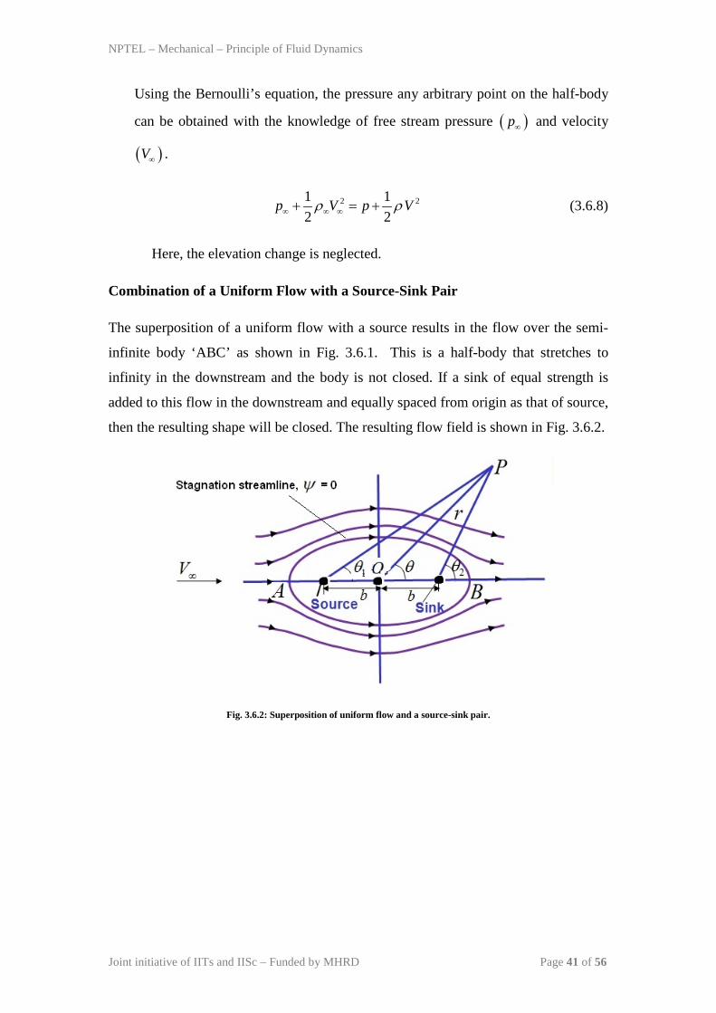
Combination of a Uniform Flow with a Source-Sink Pair
The superposition of a uniform flow with a source results in the flow over the semi-
infinite body ‘ABC’ as shown in Fig. 3.6.1. This is a half-body that stretches to
infinity in the downstream and the body is not closed. If a sink of equal strength is
added to this flow in the downstream and equally spaced from origin as that of source,
then the resulting shape will be closed. The resulting flow field is shown in Fig. 3.6.2.
Fig. 3.6.2: Superposition of uniform flow and a source-sink pair.
NPTEL – Mechanical – Principle of Fluid Dynamics
Joint initiative of IITs and IISc – Funded by MHRD Page 42 of 56
Let us consider a source and sink with strengths andΛ −Λ equally spaced at
a distance b from the origin. When a uniform stream of velocity V∞ is superimposed
on it, the combined flow at any point in the flow can be written as follow;
( )uniform source sink 1 2
12 2
12 2 2
sin2
2 sinor, sin tan2
2or, tan2
V r
brV rr bbyV y
x y b
ψ ψ ψ ψ θ θ θπ
θψ θπ
ψπ
∞
−∞
−∞
Λ= + + = + −
Λ = − − Λ
= − + −
(3.6.9)
From the geometry of Fig. 3.6.2, it is seen that 1 2andθ θ are the functions of
, andr bθ . Assigning the velocity components to zero value, two stagnation points
can be obtained in similar manner and they are located at points ‘A and B’ in the Fig.
3.6.2. Their distances from origin can also be calculated.
2
1
bOA OB l bV
lb V b
π
π
∞
∞
Λ= = = +
Λ⇒ = +
(3.6.10)
The equation of the streamline is given by,
( )1 2sin constant2
V rψ θ θ θπ∞
Λ= + − = (3.6.11)
The equation of specific streamlines passing through the stagnation points
( ) ( )1 2 1 2A and B 0θ θ θ π θ θ θ= = = = = = and B ( )1 2 0θ θ θ= = = ’ is obtained by
assigning the constant appearing in Eq. (3.6.11) as 0.
( )1 2sin 02
V rψ θ θ θπ∞
Λ= + − = (3.6.12)
NPTEL – Mechanical – Principle of Fluid Dynamics
Joint initiative of IITs and IISc – Funded by MHRD Page 43 of 56
The body-half width ( )h can be obtained by determining the value y where the y-axis
intersects streamline 0.ψ = , Thus, from Eq. (3.6.9), one can obtain the body half
width with y h= .
21 21 tan2
V bh h hb b b
π ∞ = − Λ
(3.6.13)
From the above mathematical analysis the following physical interpretation can be
made;
• The stagnation streamline described by Eq. (3.6.12), is the equation of an oval
and is the dividing streamline. This particular shape is called as “Rankine
Oval”. All the flow from the source is consumed by the sink and is contained
entirely inside the oval. The flow outside the oval is originated through
uniform flow only and can be interpreted as inviscid, irrotational and
incompressible flow over solid body. Also, the potential solution for the
Rankine oval gives the reasonable approximation of velocity outside the thin,
viscous boundary layer and pressure distribution on the front part of the body.
• Using Eqs. (3.6.10) and (3.6.13), a large variety of body shapes with different
length to width ratio can be obtained for different values of the parameter
V b∞ Λ
. As this parameter becomes large, the flow around a slender body is
described while the smaller values give the flow field around a blunt shape
body.
NPTEL – Mechanical – Principle of Fluid Dynamics
Joint initiative of IITs and IISc – Funded by MHRD Page 44 of 56
Module 3 : Lecture 7 INVISCID INCOMPRESSIBLE FLOW
(Superposition of Potential Flows - II)
Non-Lifting Flow over a Circular Cylinder
It is seen earlier that flow over a semi-infinite body can be simulated by combination
of a uniform flow with a source and flow over an oval-shaped body can be
constructed by superimposing a uniform flow and a source-sink pair. A circular
cylinder is one of the basic geometrical shapes and the flow passing over it can be
simulated by combination of a uniform flow and doublet. When the distance between
source-sink pair approaches zero, the shape Rankine oval becomes more blunt and
approaches a circular shape.
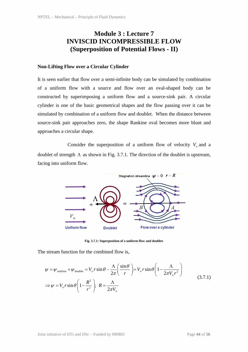
Consider the superposition of a uniform flow of velocity V∞ and a
doublet of strength Λ as shown in Fig. 3.7.1. The direction of the doublet is upstream,
facing into uniform flow.
Fig. 3.7.1: Superposition of a uniform flow and doublet.
The stream function for the combined flow is,
uniform doublet 2
2
2
sinsin sin 12 2
sin 1 ;2
V r V rr V r
RV r Rr V
θψ ψ ψ θ θπ π
ψ θπ
∞ ∞∞
∞∞
Λ Λ = + = − = −
Λ⇒ = − =
(3.7.1)
NPTEL – Mechanical – Principle of Fluid Dynamics
Joint initiative of IITs and IISc – Funded by MHRD Page 45 of 56
The velocity field is obtained as,
2 2
2 2
1 1 cos ; 1 sinrR Rv V v V
r r r rθψ ψθ θθ ∞ ∞
∂ ∂= = − = − = − + ∂ ∂
(3.7.2)
In order to locate the stagnation point, assign the velocity components in Eq. (3.7.2) to
zero value and simultaneously solve for andr θ . There are two stagnation points,
located at ( ) ( ) ( ), ,0 and ,r R Rθ π= and denoted by points A and B, respectively. The
equation of streamlines that passes through the stagnation points A and B, is given by
the following expression;
2
2sin 1 0RV rr
ψ θ∞
= − =
(3.7.3)
This equation is satisfied by r R= for all values of θ . Since R is a constant, Eq.
(3.7.3) may be interpreted as the equation of a circle with radius R with center at the
origin. It is satisfied by 0 andθ π= for all values of R . Different values of R may
be obtained by varying the uniform velocity and/or doublet strength. Hence, entire
horizontal axis through the points A and B, extending infinitely far upstream and
downstream, is a part of stagnation streamline. The above discussions can be
summarized as follows;
• The dividing streamline 0ψ = that passes through the stagnation points A and
B as shown in Fig. 3.7.1.
• The dividing streamline is a circle of radius R . The family of circles can be
obtained by assigning different values of R with various doublet strength and
free stream velocity.
• The flow inside the circle is generated from the doublet whereas flow outside
the circle comes from the uniform flow. So, the flow inside the circle may be
replaced by solid body and the external flow will not feel the difference.
• Thus, the inviscid, irrotational, incompressible flow over a circular cylinder of
radius R can be simulated by adding a uniform flow of velocity V∞ and a
doublet of strength Λ and R is related to andV∞ Λ .
2R
Vπ ∞
Λ= (3.7.4)
NPTEL – Mechanical – Principle of Fluid Dynamics
Joint initiative of IITs and IISc – Funded by MHRD Page 46 of 56
Referring to the Fig. 3.7.1, it is seen that the entire flow field is symmetrical
about both horizontal and vertical axes through the center of the cylinder. It means the
pressure distribution is also symmetrical about both the axes. When the pressure
distribution over the top part of the cylinder is exactly balanced by the bottom part,
there is no lift. Similarly, when the pressure distribution on the front part of the
cylinder is exactly balanced by rear portion, then there is no drag. This is in contrast
to the realistic situation i.e. a generic body placed in a flow field will experience finite
drag and zero lift may be possible. This paradox between the theoretical result of zero
drag in an inviscid flow and the knowledge of finite drag in real flow situation is
known as d’ Alembert’s paradox.
Pressure Coefficient
In general, pressure is a dimensional quantity. Many a times, it is expressed in a non-
dimensional form with respect to free stream flow and the ‘pressure coefficient’ is
defined as follows;
212
pp p p pc
q Vρ
∞ ∞
∞∞ ∞
− −= =
(3.7.5)
Here, and Vρ∞ ∞ are the free stream density and free stream velocity, respectively. The
term q∞ is called as dynamic pressure. For incompressible flow, if a body is
immersed in the free stream, then Bernoulli’s equation can be written at any arbitrary
point in the flow field as,
( )
2 2
2 2
2
1 12 2
12
1p
p V p V
p p V V
p p Vcq V
ρ ρ
ρ
∞ ∞ ∞
∞ ∞
∞
∞ ∞
+ = +
⇒ − = −
−⇒ = = −
(3.7.6)
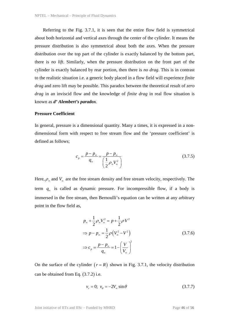
On the surface of the cylinder ( )r R= shown in Fig. 3.7.1, the velocity distribution
can be obtained from Eq. (3.7.2) i.e.
0; 2 sinrv v Vθ θ∞= = − (3.7.7)
NPTEL – Mechanical – Principle of Fluid Dynamics
Joint initiative of IITs and IISc – Funded by MHRD Page 47 of 56
Fig. 3.7.2: Maximum velocity in the flow over a circular cylinder.
Here, rv is geometrically normal to the surface and vθ
is tangential to the surface of
the cylinder as shown in Fig. 3.7.2(a). The negative sign signifies that vθ is positive
in the direction of increasing θ . It may be observed that the velocity at the surface
reaches to maximum value of 2V∞ at the top and bottom of the cylinder as shown in
Fig. 3.7.2(b). Eqs. (3.7.6) and (3.7.7) can be combined to obtain the surface pressure
coefficient as,
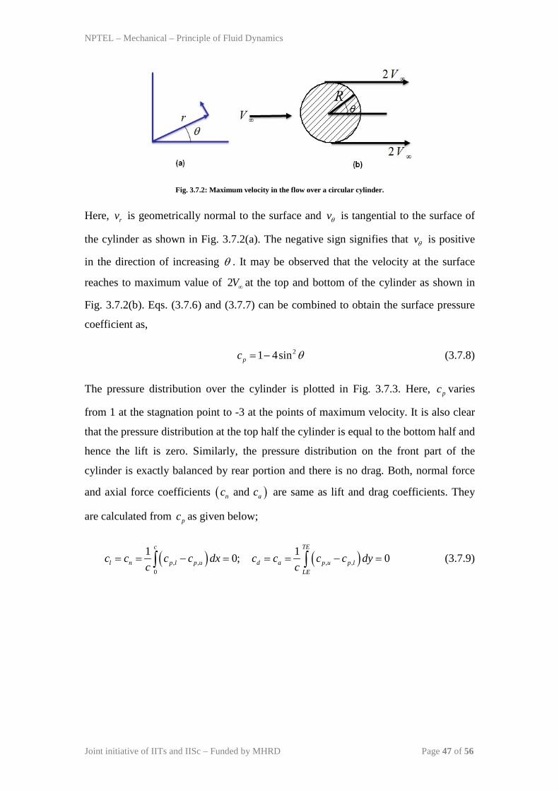
21 4sinpc θ= − (3.7.8)
The pressure distribution over the cylinder is plotted in Fig. 3.7.3. Here, pc varies
from 1 at the stagnation point to -3 at the points of maximum velocity. It is also clear
that the pressure distribution at the top half the cylinder is equal to the bottom half and
hence the lift is zero. Similarly, the pressure distribution on the front part of the
cylinder is exactly balanced by rear portion and there is no drag. Both, normal force
and axial force coefficients ( )andn ac c are same as lift and drag coefficients. They
are calculated from pc as given below;
( ) ( ), , , ,0
1 10; 0c TE
l n p l p u d a p u p lLE
c c c c dx c c c c dyc c
= = − = = = − =∫ ∫ (3.7.9)
NPTEL – Mechanical – Principle of Fluid Dynamics
Joint initiative of IITs and IISc – Funded by MHRD Page 48 of 56
Here, LE and TE stands for leading edge and trailing edge, respectively. The
subscripts u and l refers to upper and lower surface of the cylinder. The chord c is the
diameter of the cylinder ( )R .
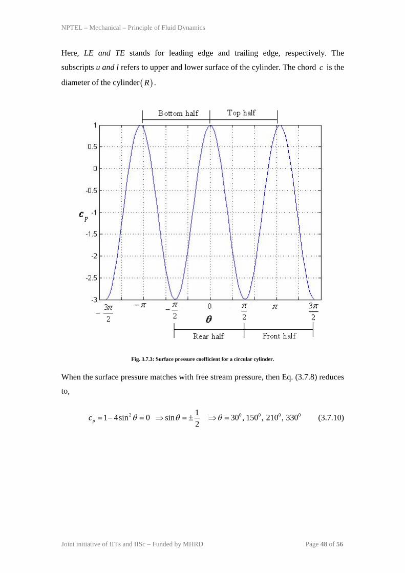
Fig. 3.7.3: Surface pressure coefficient for a circular cylinder.
When the surface pressure matches with free stream pressure, then Eq. (3.7.8) reduces
to,
2 0 0 0 011 4sin 0 sin 30 , 150 , 210 , 3302pc θ θ θ= − = ⇒ = ± ⇒ = (3.7.10)
NPTEL – Mechanical – Principle of Fluid Dynamics
Joint initiative of IITs and IISc – Funded by MHRD Page 49 of 56
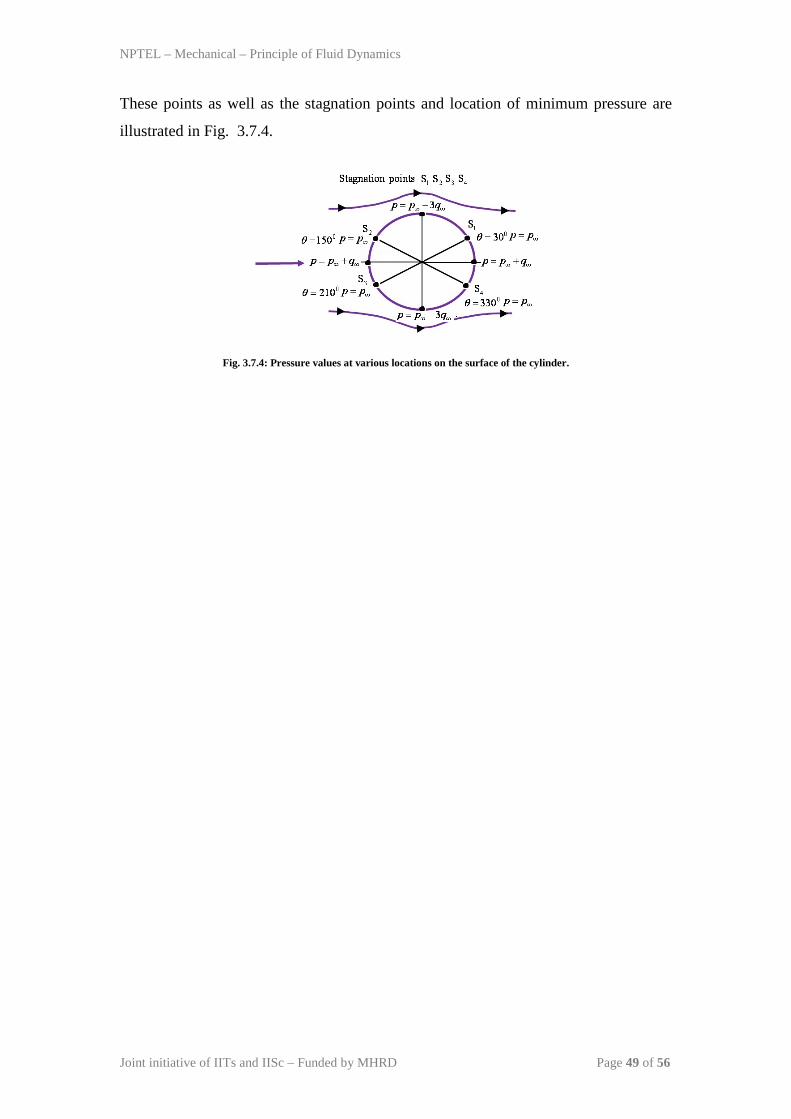
These points as well as the stagnation points and location of minimum pressure are
illustrated in Fig. 3.7.4.
Fig. 3.7.4: Pressure values at various locations on the surface of the cylinder.
NPTEL – Mechanical – Principle of Fluid Dynamics
Joint initiative of IITs and IISc – Funded by MHRD Page 50 of 56
Module 3 : Lecture 8 INVISCID INCOMPRESSIBLE FLOW (Superposition of Potential Flows - III)
Lifting Flow over a Circular Cylinder
When a doublet flow is superimposed on a uniform flow, the combined flow fields
can be visualized as possible flow pattern over a circular cylinder. In addition, both
lift and drag force are zero for such flows. However, there are other possible flow
patterns around a circular cylinder resulting non-zero lift. Such lifting flows are
discussed here.
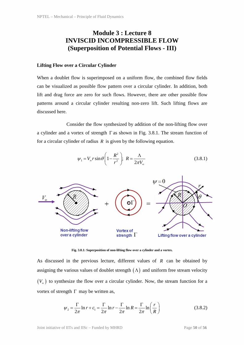
Consider the flow synthesized by addition of the non-lifting flow over
a cylinder and a vortex of strength Γ as shown in Fig. 3.8.1. The stream function of
for a circular cylinder of radius R is given by the following equation.
2
1 2sin 1 ;2
RV r Rr V
ψ θπ∞
∞
Λ= − =
(3.8.1)
Fig. 3.8.1: Superposition of non-lifting flow over a cylinder and a vortex.
As discussed in the previous lecture, different values of R can be obtained by
assigning the various values of doublet strength ( )Λ and uniform free stream velocity
( )V∞ to synthesize the flow over a circular cylinder. Now, the stream function for a
vortex of strength Γ may be written as,
2 1ln ln ln ln2 2 2 2
rr c r RR
ψπ π π πΓ Γ Γ Γ = + = − =
(3.8.2)
NPTEL – Mechanical – Principle of Fluid Dynamics
Joint initiative of IITs and IISc – Funded by MHRD Page 51 of 56
Since 1c is any arbitrary constant, it can be replaced with ln2
RπΓ −
in the Eq.
(3.8.2). The resulting stream function for the flow pattern is given by the sum of the
stream functions, i.e.
2
1 2 2sin 1 ln2
R rV rr R
ψ ψ ψ θπ∞
Γ = + = − +
(3.8.3)
The streamlines expressed by Eq. (3.8.3), represents the equation of a circle of radius
R . A special case will arise that will represent the flow over a circular cylinder when
0Γ = . If r R= then 0ψ = for all values of θ . The velocity fields can be obtained
by differentiating Eq. (3.8.3) i.e.
2
2
2
2
1 1 cos
1 sin2
rRv V
r r
Rv Vr r rθ
ψ θθ
ψ θπ
∞
∞
∂= = − ∂
∂ Γ= − = − + − ∂
(3.8.4)
In order to locate the stagnation points, one can put 0rv vθ= = in Eq. (3.8.4) and
solve for resulting coordinates ( ),r θ :
sin4
r RV R
θπ ∞
Γ= ⇒ = −
(3.8.5)
Since Γ is a positive number, the value of θ must be lie in the range and 2π π and
there are three possibilities;
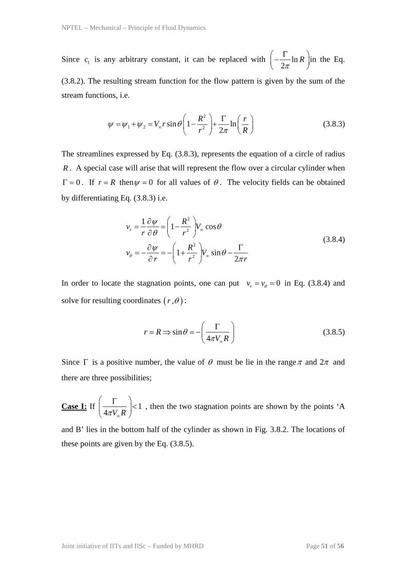
Case I: If 14 V Rπ ∞
Γ<
, then the two stagnation points are shown by the points ‘A
and B’ lies in the bottom half of the cylinder as shown in Fig. 3.8.2. The locations of
these points are given by the Eq. (3.8.5).
NPTEL – Mechanical – Principle of Fluid Dynamics
Joint initiative of IITs and IISc – Funded by MHRD Page 52 of 56
Case II: If 14 V Rπ ∞
Γ=
, then there is one stagnation point on the surface of the
cylinder at the point ‘C’ as shown in Fig. 3.8.2. It means that the point ‘A and B’
come closer meet at point ‘C’ on the surface at and2
r R πθ= = − .
Case III: When, 14 V Rπ ∞
Γ>
, no interpretation can be made from Eq. (3.8.5).
Referring to Eq. (3.8.4), the stagnation point 0rv = is satisfied for both
and or2 2
r R π πθ= = − . Now, substitute 2πθ = − in Eq. (3.8.4) and solve for r by
setting 0vθ = at the stagnation point.
22
4 4r R
V Vπ π∞ ∞
Γ Γ= ± −
(3.8.6)
Eq. (3.8.6) is a quadratic equation and the two possible solutions can be interpreted as
stagnation points: one lies inside the cylinder (point ‘D’) and other lies outside the
cylinder (point ‘E’) as shown in Fig. 3.8.2. Physically, the point ‘D’ is generated
within the cylinder r R< , when a doublet flow at origin is superimposed on a vortex
flow while the point ‘E’ lies on same vertical axis for r R> .
Fig. 3.8.2: Stagnation points for lifting flow over a cylinder.
NPTEL – Mechanical – Principle of Fluid Dynamics
Joint initiative of IITs and IISc – Funded by MHRD Page 53 of 56
Based on the results shown in Fig. 3.8.2, the following inferences can be made;
• The circular streamline 0 and r Rψ = = is one of the allowed streamline in
the synthesized flow field that divides the doublet flow and vortex flow. So,
one can replace it as a solid body i.e. circular cylinder and the external flow
will not feel the difference. The free stream can be considered as a vortex
flow.
• With reference to the solid body, the stagnation point ‘D’ has no meaning and
only point ‘E” is the meaningful stagnation point.
• Since, the parameter Γ can be chosen freely, there are infinite numbers of
possible potential flow solutions, for incompressible flow over a circular
cylinder. This is also true for incompressible potential flows over all smooth
two-dimensional bodies.
Lift and Drag Coefficients for Circular Cylinder
Intuitively, one can say that there is a finite normal force when a circular cylinder is
placed in a vortex flow while the drag is zero i.e. d’Alembert’s paradox still prevails.
Let us quantify the results;
First, the velocity on the surface of the cylinder ( )r R= can be written as,
2 sin2
V v VRθ θ
π∞
Γ= = − − (3.8.7)
The pressure coefficient is obtained as,
2 2 22 2 sin1 1 2sin 1 4sin
2 2pVcV RV RV RV
θθ θπ π π∞ ∞ ∞ ∞
Γ Γ Γ = − = − − − = − + +
(3.8.8)
NPTEL – Mechanical – Principle of Fluid Dynamics
Joint initiative of IITs and IISc – Funded by MHRD Page 54 of 56
The force coefficients can be obtained by integrating pressure coefficient and skin
friction coefficient over the surface. For the inviscid flow, there is no skin friction
coefficient. Hence, the drag coefficient is written as,
( ), , , ,1 1 1
2 2 2
TE TE TE
d p l p u p u p lLE LE LE
c c c dy c dy c dyR R R
= − = −∫ ∫ ∫ (3.8.9)
Converting Eq. (3.8.9) to polar coordinates by replacing sin ; cosy R dy R dθ θ θ= = ,
we can obtain,
0 2
, ,1 1cos cos2 2d p u p lc c d c d
π
π π
θ θ θ θ= −∫ ∫ (3.8.10)
Here, the first part of integration is performed from the leading edge (i.e. front point)
and moving over the top surface. In the second part, the integration is done from the
leading edge moving over the bottom portion of the cylinder. Finally, Eq. (3.8.10) can
be written as,
0 2 2
0
1 1 1cos cos cos2 2 2d p p pc c d c d c d
π π
π π
θ θ θ θ θ θ= − − = −∫ ∫ ∫ (3.8.11)
Substitute the value of pc from Eq.(3.8.8) in Eq.(3.8.11),
222
0
1 2 sin1 4sin cos2 2dc d
RV RV
π θθ θ θπ π∞ ∞
Γ Γ = − − + +
∫ (3.8.12)
Use the following trigonometric relations in Eq. (3.8.12);
2 2 22
0 0 0
cos 0; sin cos 0; sin cos 0d dπ π π
θ θ θ θ θ θ θ= = =∫ ∫ ∫ (3.8.13)
It leads to 0dc = , which implies that the drag on a cylinder in an inviscid,
incompressible flow is zero, regardless of whether or not the flow has circulation
about the cylinder. The lift can be evaluated in the similar manner from the first
principle i.e.
( )2 2 2
, , , ,0 0 0
1 1 12 2 2
R R R
l p l p u p l p uc c c dx c dx c dxR R R
= − = −∫ ∫ ∫ (3.8.14)
NPTEL – Mechanical – Principle of Fluid Dynamics
Joint initiative of IITs and IISc – Funded by MHRD Page 55 of 56
Converting Eq. (3.8.14) to polar coordinates by replacing
cos ; sinx R dx R dθ θ θ= = − , we can obtain,
2 0 2
, ,0
1 1 1sin sin sin2 2 2l p l p u pc c d c d c d
π π
π π
θ θ θ θ θ θ= − + = −∫ ∫ ∫ (3.8.15)
Substitute the value of pc from Eq.(3.8.8) in Eq.(3.8.15),
222
0
1 2 sin1 4sin sin2 2lc d
RV RV
π θθ θ θπ π∞ ∞
Γ Γ = − − + +
∫ (3.8.16)
Use the following trigonometric relations in Eq. (3.8.16);
2 2 22 3
0 0 0
sin 0; sin ; sin 0d dπ π π
θ θ θ π θ θ= = =∫ ∫ ∫ (3.8.17)
The lift coefficient can be obtained as,
212
lLc
RV RVV Sρ∞ ∞∞ ∞
′Γ Γ= ⇒ =
(3.8.18)
The value of lift per unit span ( )L′ can be obtained by considering the plan-form area
2S R= in Eq. (3.8.18) and after simplification, one can obtain,
L Vρ∞ ∞′ = Γ (3.8.19)
It is seen from Eq.(3.8.19) that the lift per unit span for a circular cylinder in a given
free stream flow is directly proportional to the circulation. This simple and powerful
relation is known as Kutta-Joukowski theorem. This result shows the importance of
the concept circulation and the same result can be extended for two-dimensional
bodies. The inviscid potential flow does not provide proper explanation for drag
calculation because zero drag in a flow field is quite un-realistic. Because of viscous
effects the flow separates from the rear part of the cylinder, creating recirculating flow
in the wake downstream of the body. This separated flow greatly contributes the finite
drag measured for the cylinder. However, the prediction of lift by Kutta-Joukowski
theorem is quite realistic.
NPTEL – Mechanical – Principle of Fluid Dynamics
Joint initiative of IITs and IISc – Funded by MHRD Page 56 of 56
Magnus Effect
The general idea of generation of lift for a spinning circular cylinder can be extended
to sphere. Here, non-symmetric flows are generated due to spinning of bodies in all
dimensions. It leads to the generation of aerodynamic force perpendicular to the
body’s angular velocity vector. This phenomenon is called as Magnus effect. The
typical examples include the spinning of three-dimensional object such as soccer,
tennis and golf balls where the side force is experienced.


![Rieb diplomado mod3[1]](https://img.pdfslide.net/doc/110x75/54847172b4af9fd2568b49e8/rieb-diplomado-mod31.jpg)