1

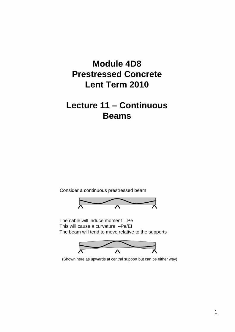
Module 4D8Prestressed Concrete

Lent Term 2010

Lecture 11 – Continuous Beams

Consider a continuous prestressed beam

The cable will induce moment –PeThis will cause a curvature –Pe/EIThe beam will tend to move relative to the supports

(Shown here as upwards at central support but can be either way)

2

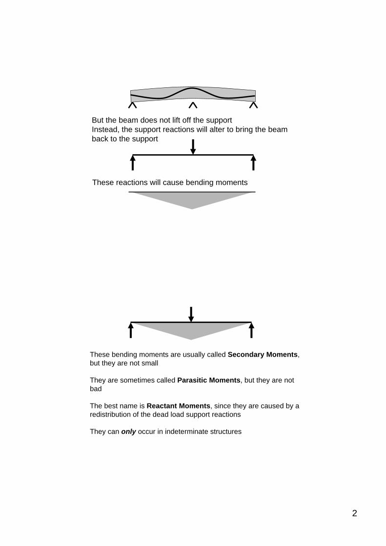
But the beam does not lift off the supportInstead, the support reactions will alter to bring the beam back to the support

These reactions will cause bending moments

These bending moments are usually called Secondary Moments, but they are not small

They are sometimes called Parasitic Moments, but they are not bad

The best name is Reactant Moments, since they are caused by a redistribution of the dead load support reactions

They can only occur in indeterminate structures

3

Reactant Moments• Reactant moments are not necessarily small –

they can easily be about 50% of the dead load moments but are distributed differently

• Reactant moments are not bad• Good designers use them to assist with the design

• Most designers try to minimise them to avoid complications

• Bad designers ignore them, which is very dangerous – the moments are real and can cause very large forces

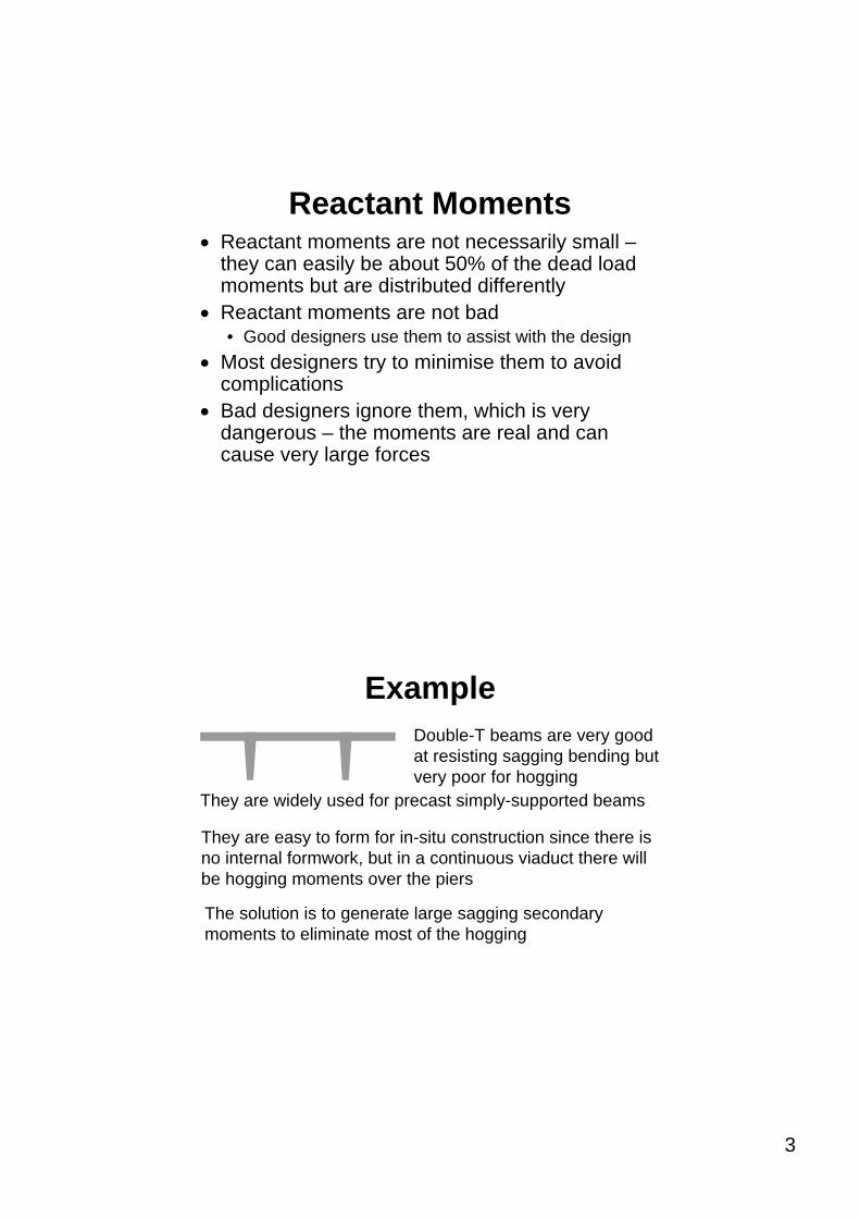
ExampleDouble-T beams are very good at resisting sagging bending but very poor for hogging

They are widely used for precast simply-supported beams

They are easy to form for in-situ construction since there is no internal formwork, but in a continuous viaduct there will be hogging moments over the piers

The solution is to generate large sagging secondary moments to eliminate most of the hogging

4

Effect of prestressWe need to define two cable profiles• es is the actual cable profileThe primary moment caused by the prestress

itself is – PesThere are also secondary moments M2So the total effect of the prestress is

– Pes + M2 = – Pepep is the place where the cable appears to act• ep is known as the line of thrust of the cable

ep or es ?• It is the total effect of the prestress (i.e. the line

of thrust ep) which must satisfy the stress inequalities, and thus which must be plotted on the Magnel diagram

• But ep can only be found by analysing the whole cable profile

• So paradox – you need to know es before you can find ep to enable you to design the prestress at a cross-section

• We must find a sensible way to design these structures

5

Constraints• The line of thrust ep must satisfy the stress

limits• but it need not lie wholly within the section

since it is only a notional line• The actual cable profile must lie within the

section and be subject to limits on the cover

• This gives great freedom to the designer

Calculate ep for a given es

There are two methods for analysing a cable profile

1. Equivalent load method – calculate the forces the cable causes on the beam and analyse

2. Virtual WorkWe can then devise methods for

designing the beams

6

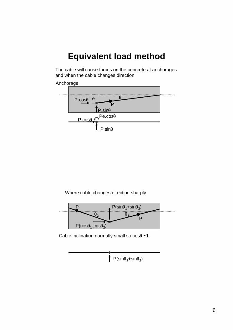
θeP

Anchorage

Equivalent load methodThe cable will cause forces on the concrete at anchorages and when the cable changes direction

P.sinθ

P.cosθ

P.sinθ

P.cosθPe.cosθ

θ1P

θ2

P P(sinθ1+sinθ2)

P(cosθ1-cosθ2)

Where cable changes direction sharply

Cable inclination normally small so cosθ ~1

P(sinθ1+sinθ2)

7

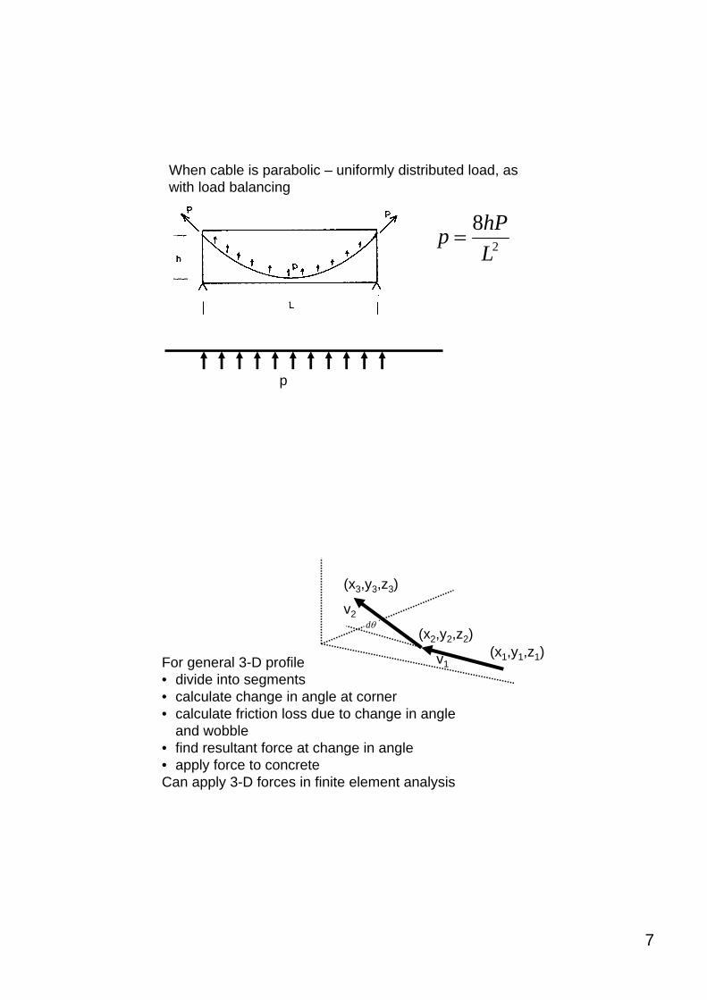
2

8LhPp =

When cable is parabolic – uniformly distributed load, as with load balancing

p

(x1,y1,z1)(x2,y2,z2)

(x3,y3,z3)

θd

v1

v2

For general 3-D profile • divide into segments • calculate change in angle at corner• calculate friction loss due to change in angle

and wobble• find resultant force at change in angle• apply force to concreteCan apply 3-D forces in finite element analysis

8

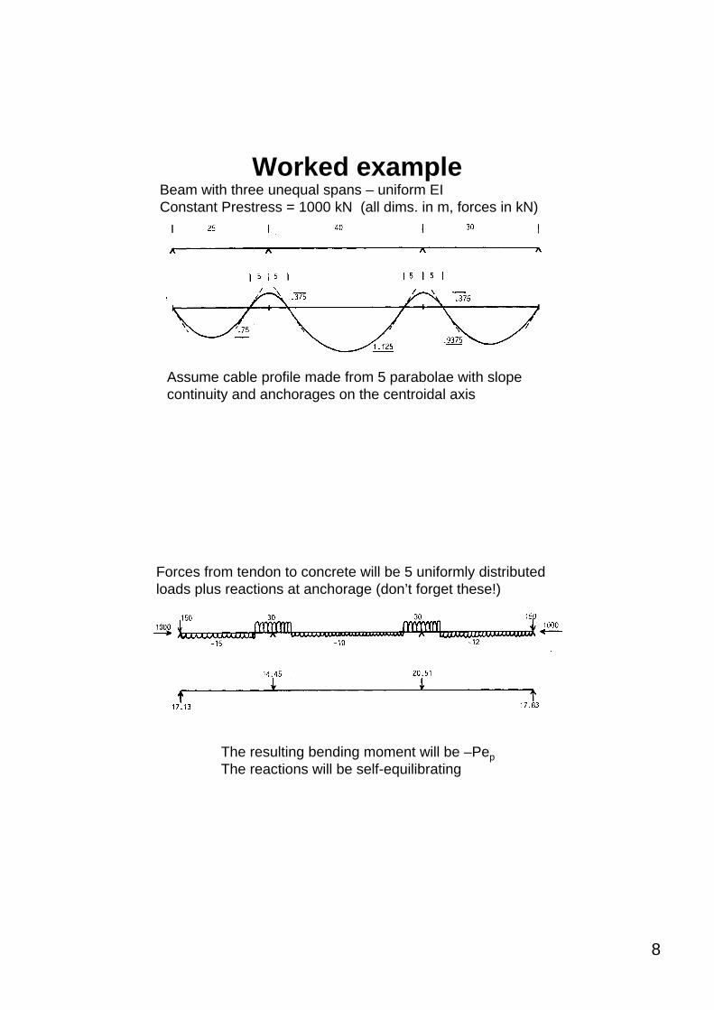
Worked exampleBeam with three unequal spans – uniform EIConstant Prestress = 1000 kN (all dims. in m, forces in kN)

Assume cable profile made from 5 parabolae with slope continuity and anchorages on the centroidal axis

Forces from tendon to concrete will be 5 uniformly distributed loads plus reactions at anchorage (don’t forget these!)

The resulting bending moment will be –PepThe reactions will be self-equilibrating

9

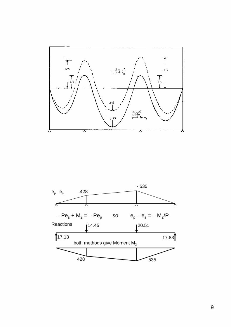
– Pes + M2 = – Pep so ep – es = – M2/P

ep - es -.428-.535

14.45 20.51

17.13 17.83

Reactions

both methods give Moment M2

428 535

10

Linear Transformation• M2 is caused by a redistribution of the

support reactions• It must be zero at end simple supports

(and in any cantilever overhangs)• It must vary linearly between supports• If P is constant, then ep – es must also vary

linearly between supports• This is known as a linear transformation

of the cable profile

Use of Linear Transformation• If we have a cable profile (es) and/or its

corresponding line of thrust (ep), then:-• We can vary es by any linear transformation, and

the line of thrust will not alter• We will have changed the indeterminate support

reactions, but not the total effect of the cable• This gives great freedom to the designer; once a

satisfactory ep or es has been found, linear transformations can be applied at will, for example to fit the tendon into the section

11

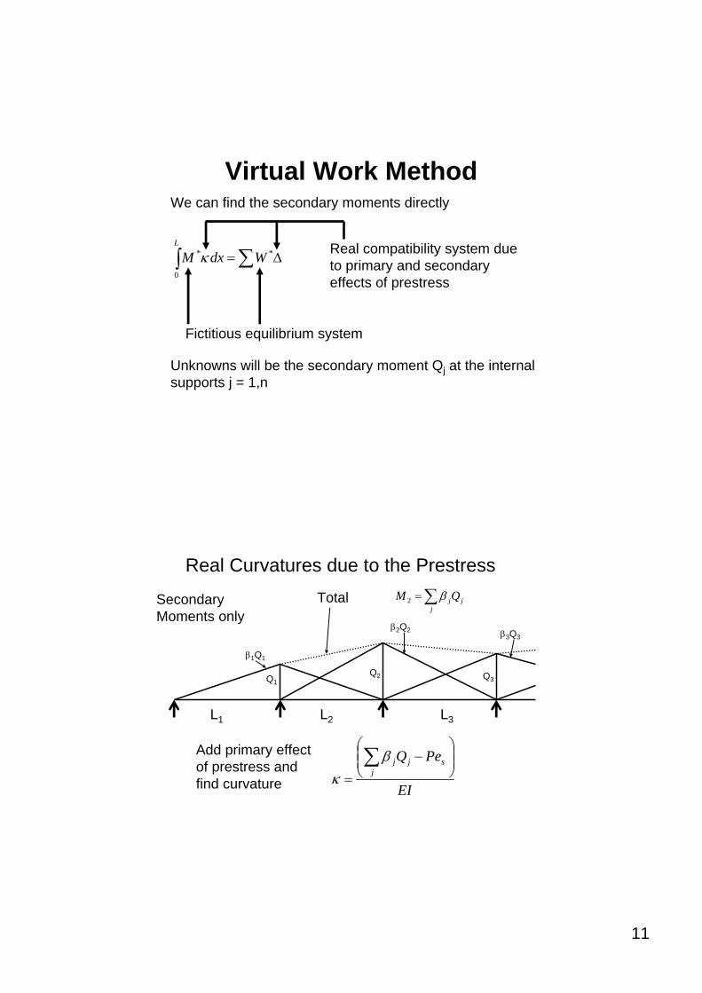
Virtual Work Method

∫ ∑ Δ=L

WdxM0

**κ

We can find the secondary moments directly

Real compatibility system due to primary and secondary effects of prestress

Fictitious equilibrium system

Unknowns will be the secondary moment Qj at the internal supports j = 1,n

L1 L3L2

Q1

β1Q1

Q2

β2Q2

Q3

β3Q3

Total ∑=j

jjQM β2

Real Curvatures due to the Prestress

EI

PeQ sj

jj ⎟⎟⎠

⎞⎜⎜⎝

⎛−

=∑β

κ

Add primary effect of prestress and find curvature

Secondary Moments only

12

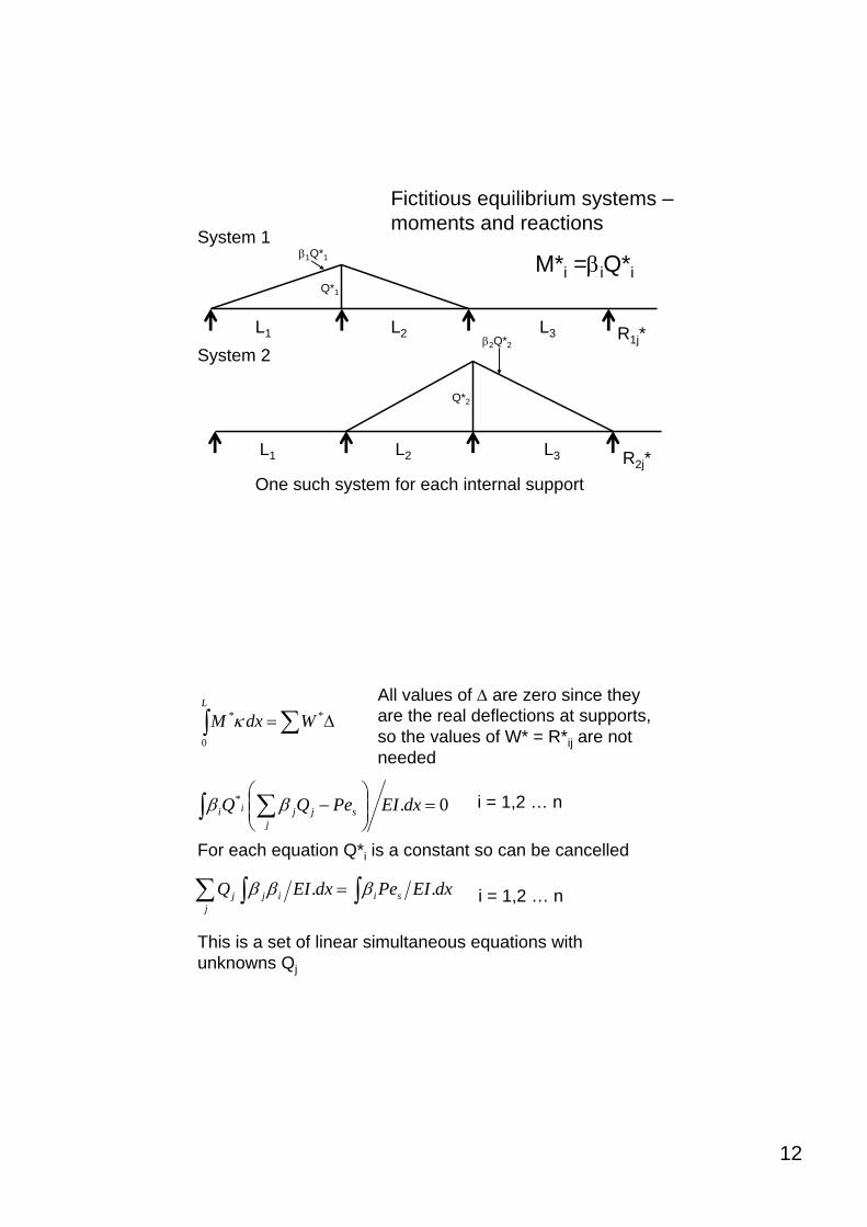
Q*1

β1Q*1

R1j*

Q*2

β2Q*2

R2j*

Fictitious equilibrium systems –moments and reactions

L1 L3L2

System 1

L1 L3L2

System 2

M*i =βiQ*i

One such system for each internal support

∫ ∑ Δ=L

WdxM0

**κAll values of Δ are zero since they are the real deflections at supports, so the values of W* = R*ij are not needed

0.* =⎟⎟⎠

⎞⎜⎜⎝

⎛−∫ ∑ dxEIPeQQ s

jjjii ββ i = 1,2 … n

For each equation Q*i is a constant so can be cancelled

∫∫∑ = dxEIPedxEIQ siijj

j .. βββ i = 1,2 … n

This is a set of linear simultaneous equations with unknowns Qj

13

⎥⎥⎥

⎦

⎤

⎢⎢⎢

⎣

⎡=

⎥⎥⎥

⎦

⎤

⎢⎢⎢

⎣

⎡

⎥⎥⎥

⎦

⎤

⎢⎢⎢

⎣

⎡

∫∫M

M

M

LLL

LL

LLL

dxEIPeQ

QdxEI si

n

ji ..1

βββ

Solve for Qi

⎥⎥⎥

⎦

⎤

⎢⎢⎢

⎣

⎡=

⎥⎥⎥

⎦

⎤

⎢⎢⎢

⎣

⎡

⎥⎥⎥

⎦

⎤

⎢⎢⎢

⎣

⎡

∫∫M

M

M

LLL

LL

LLL

dxPeQ

Qdx si

n

ji ..1

βββ

Iff EI is constant, then

Many of the terms in the l.h.matrix will be zero since either βior βj will be zero

βiβj

siLi

For j = i -1

6

.1.

i

iiji

L

dsLs

Lsdx

=

⎟⎟⎠

⎞⎜⎜⎝

⎛−=∫ ∫ββ

6. 1+∫ = i

jiLdxββSimilarly, if j = i + 1

14

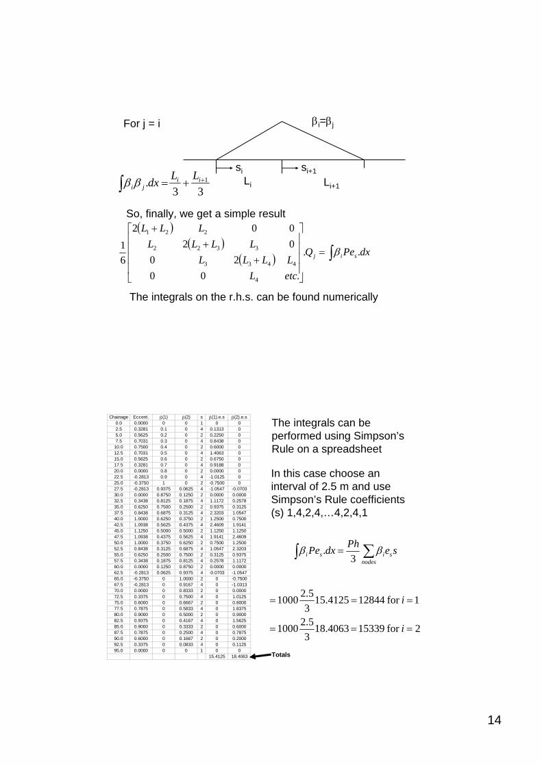
For j = i βi=βj

siLi

si+1

Li+133. 1++=∫ ii

jiLLdxββ

( )( )

( ) ∫=⎥⎥⎥⎥

⎦

⎤

⎢⎢⎢⎢

⎣

⎡

++

+

dxPeQ

etcLLLLL

LLLLLLL

sij ..

.0020

02002

61

4

4433

3322

221

β

So, finally, we get a simple result

The integrals on the r.h.s. can be found numerically

The integrals can be performed using Simpson’s Rule on a spreadsheet

In this case choose an interval of 2.5 m and use Simpson’s Rule coefficients (s) 1,4,2,4,…4,2,4,1

Chainage Eccent. β(1) β(2) s β(1).e.s β(2).e.s0.0 0.0000 0 0 1 0 02.5 0.3281 0.1 0 4 0.1313 05.0 0.5625 0.2 0 2 0.2250 07.5 0.7031 0.3 0 4 0.8438 0

10.0 0.7500 0.4 0 2 0.6000 012.5 0.7031 0.5 0 4 1.4063 015.0 0.5625 0.6 0 2 0.6750 017.5 0.3281 0.7 0 4 0.9188 020.0 0.0000 0.8 0 2 0.0000 022.5 -0.2813 0.9 0 4 -1.0125 025.0 -0.3750 1 0 2 -0.7500 027.5 -0.2813 0.9375 0.0625 4 -1.0547 -0.070330.0 0.0000 0.8750 0.1250 2 0.0000 0.000032.5 0.3438 0.8125 0.1875 4 1.1172 0.257835.0 0.6250 0.7500 0.2500 2 0.9375 0.312537.5 0.8438 0.6875 0.3125 4 2.3203 1.054740.0 1.0000 0.6250 0.3750 2 1.2500 0.750042.5 1.0938 0.5625 0.4375 4 2.4609 1.914145.0 1.1250 0.5000 0.5000 2 1.1250 1.125047.5 1.0938 0.4375 0.5625 4 1.9141 2.460950.0 1.0000 0.3750 0.6250 2 0.7500 1.250052.5 0.8438 0.3125 0.6875 4 1.0547 2.320355.0 0.6250 0.2500 0.7500 2 0.3125 0.937557.5 0.3438 0.1875 0.8125 4 0.2578 1.117260.0 0.0000 0.1250 0.8750 2 0.0000 0.000062.5 -0.2813 0.0625 0.9375 4 -0.0703 -1.054765.0 -0.3750 0 1.0000 2 0 -0.750067.5 -0.2813 0 0.9167 4 0 -1.031370.0 0.0000 0 0.8333 2 0 0.000072.5 0.3375 0 0.7500 4 0 1.012575.0 0.6000 0 0.6667 2 0 0.800077.5 0.7875 0 0.5833 4 0 1.837580.0 0.9000 0 0.5000 2 0 0.900082.5 0.9375 0 0.4167 4 0 1.562585.0 0.9000 0 0.3333 2 0 0.600087.5 0.7875 0 0.2500 4 0 0.787590.0 0.6000 0 0.1667 2 0 0.200092.5 0.3375 0 0.0833 4 0 0.112595.0 0.0000 0 0 1 0 0

15.4125 18.4063

2for 153394063.1835.21000

1for 128444125.1535.21000

===

===

i

i

sePhdxPenodes

sisi ∑∫ = ββ3

.

Totals

15

⎥⎦

⎤⎢⎣

⎡=⎥

⎦

⎤⎢⎣

⎡

⎥⎦

⎤⎢⎣

⎡=⎥

⎦

⎤⎢⎣

⎡⎥⎦

⎤⎢⎣

⎡+

+

04.53516.428

1533912844

)3040(24040)4025(2

61

2

1

2

1

QQ

QQ

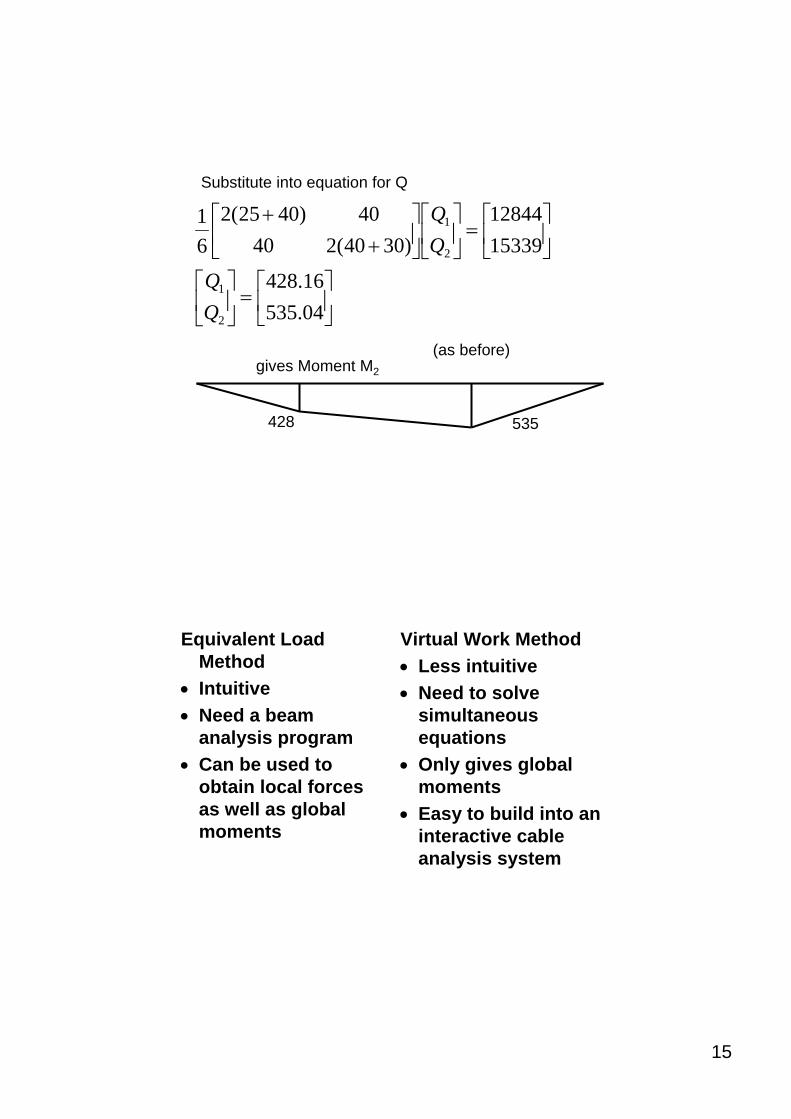
gives Moment M2

428 535

Substitute into equation for Q

(as before)

Equivalent Load Method

• Intuitive• Need a beam

analysis program• Can be used to

obtain local forces as well as global moments

Virtual Work Method• Less intuitive• Need to solve

simultaneous equations

• Only gives global moments

• Easy to build into an interactive cable analysis system

16

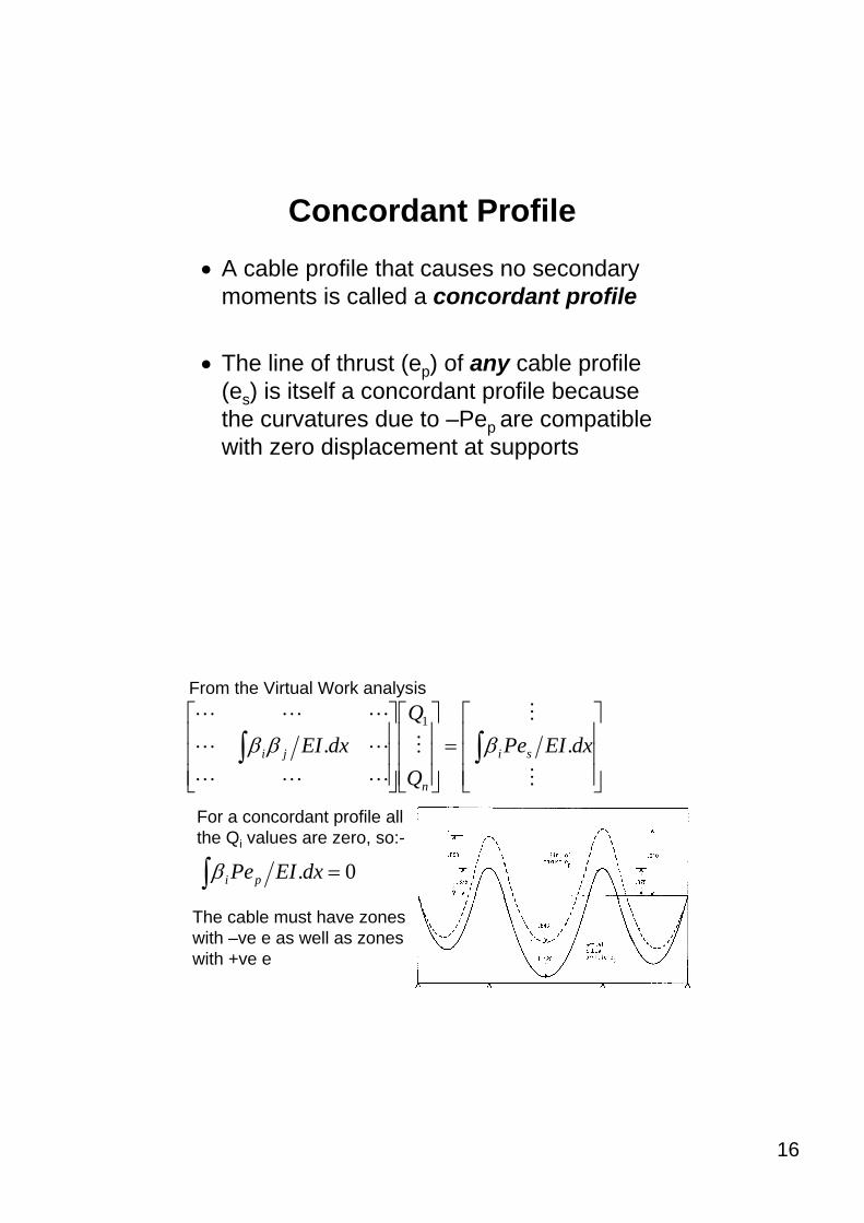
Concordant Profile• A cable profile that causes no secondary

moments is called a concordant profile

• The line of thrust (ep) of any cable profile (es) is itself a concordant profile because the curvatures due to –Pep are compatible with zero displacement at supports

⎥⎥⎥

⎦

⎤

⎢⎢⎢

⎣

⎡=

⎥⎥⎥

⎦

⎤

⎢⎢⎢

⎣

⎡

⎥⎥⎥

⎦

⎤

⎢⎢⎢

⎣

⎡

∫∫M

M

M

LLL

LL

LLL

dxEIPeQ

QdxEI si

n

ji ..1

βββ

From the Virtual Work analysis

For a concordant profile all the Qi values are zero, so:-

0. =∫ dxEIPepiβ

The cable must have zones with –ve e as well as zones with +ve e

17

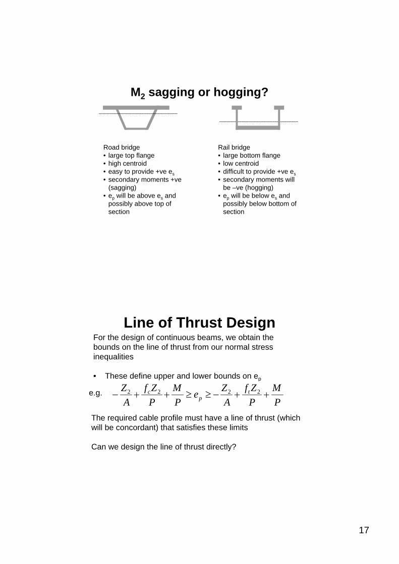
M2 sagging or hogging?

Road bridge • large top flange• high centroid• easy to provide +ve es• secondary moments +ve

(sagging)• ep will be above es and

possibly above top of section

Rail bridge• large bottom flange• low centroid• difficult to provide +ve es• secondary moments will

be –ve (hogging)• ep will be below es and

possibly below bottom of section

Line of Thrust DesignFor the design of continuous beams, we obtain the bounds on the line of thrust from our normal stress inequalities

• These define upper and lower bounds on ep

The required cable profile must have a line of thrust (which will be concordant) that satisfies these limits

Can we design the line of thrust directly?

PM

PZf

AZe

PM

PZf

AZ t

pc ++−≥≥++− 2222e.g.

18

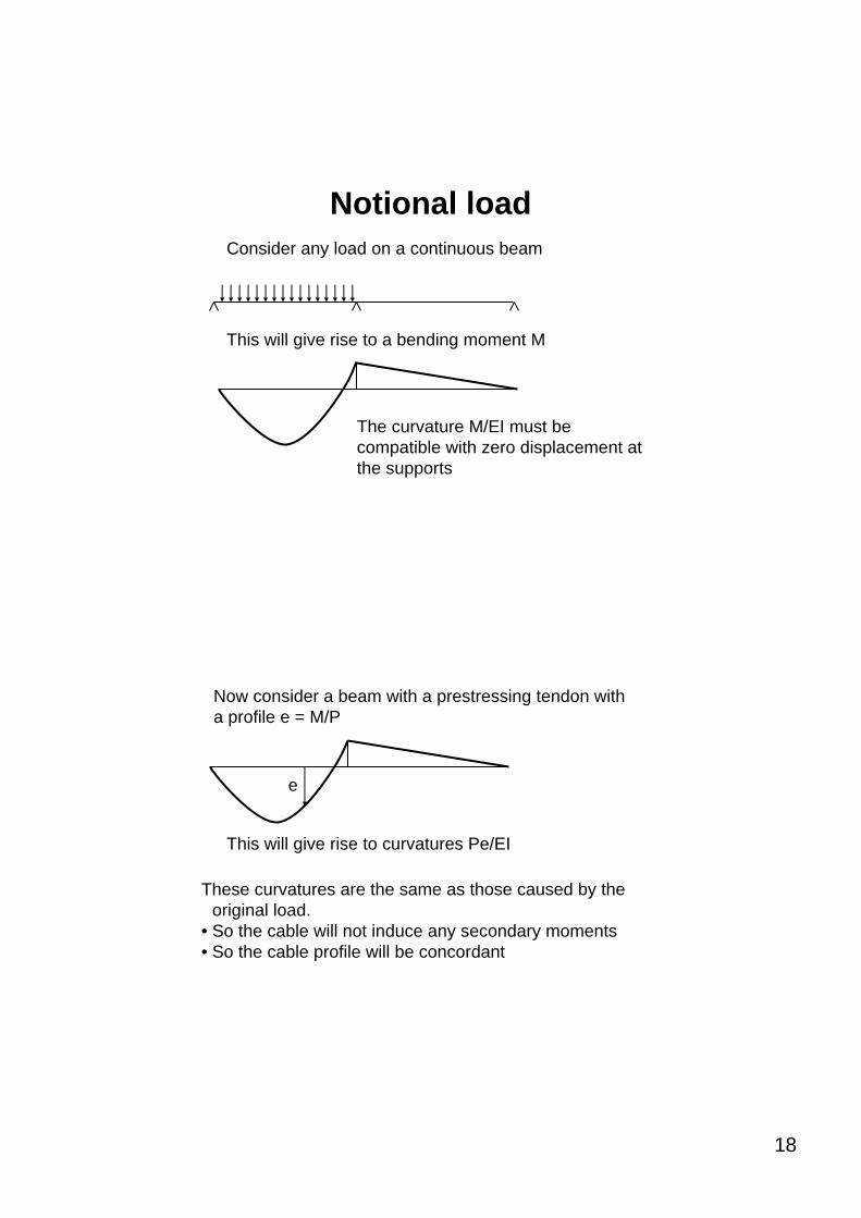
Notional loadConsider any load on a continuous beam

This will give rise to a bending moment M

The curvature M/EI must be compatible with zero displacement at the supports

Now consider a beam with a prestressing tendon with a profile e = M/P

e

This will give rise to curvatures Pe/EI

These curvatures are the same as those caused by the original load.

• So the cable will not induce any secondary moments• So the cable profile will be concordant

19

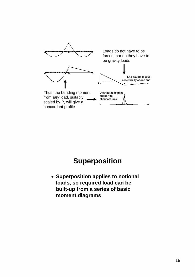
Thus, the bending moment from any load, suitably scaled by P, will give a concordant profile

Loads do not have to be forces, nor do they have to be gravity loads

End couple to give eccentricity at one end

Distributed load at support to eliminate kink

Superposition

• Superposition applies to notional loads, so required load can be built-up from a series of basic moment diagrams

20

Finding line of thrust• So the selection of a line of thrust that

satisfies the limits on ep is equivalent to finding a notional load whose bending moment M, when scaled by the prestressing force P, satisfies those limits

• Note that the notional loading has nothing to do with the real load on the structure

Automated Design of ep

• It is relatively easy to design a suitable profile, since most engineers have a feel for the loads needed to cause a bending moment at a given point

• The process can be automated by using an iterative procedure

21

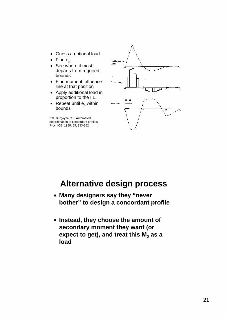
• Guess a notional load• Find ep• See where it most

departs from required bounds

• Find moment influence line at that position

• Apply additional load in proportion to the I.L.

• Repeat until ep within bounds

Ref. Burgoyne C J, Automated determination of concordant profilesProc. ICE, 1988, 85, 333-352

Alternative design process• Many designers say they “never

bother” to design a concordant profile

• Instead, they choose the amount of secondary moment they want (or expect to get), and treat this M2 as a load

22

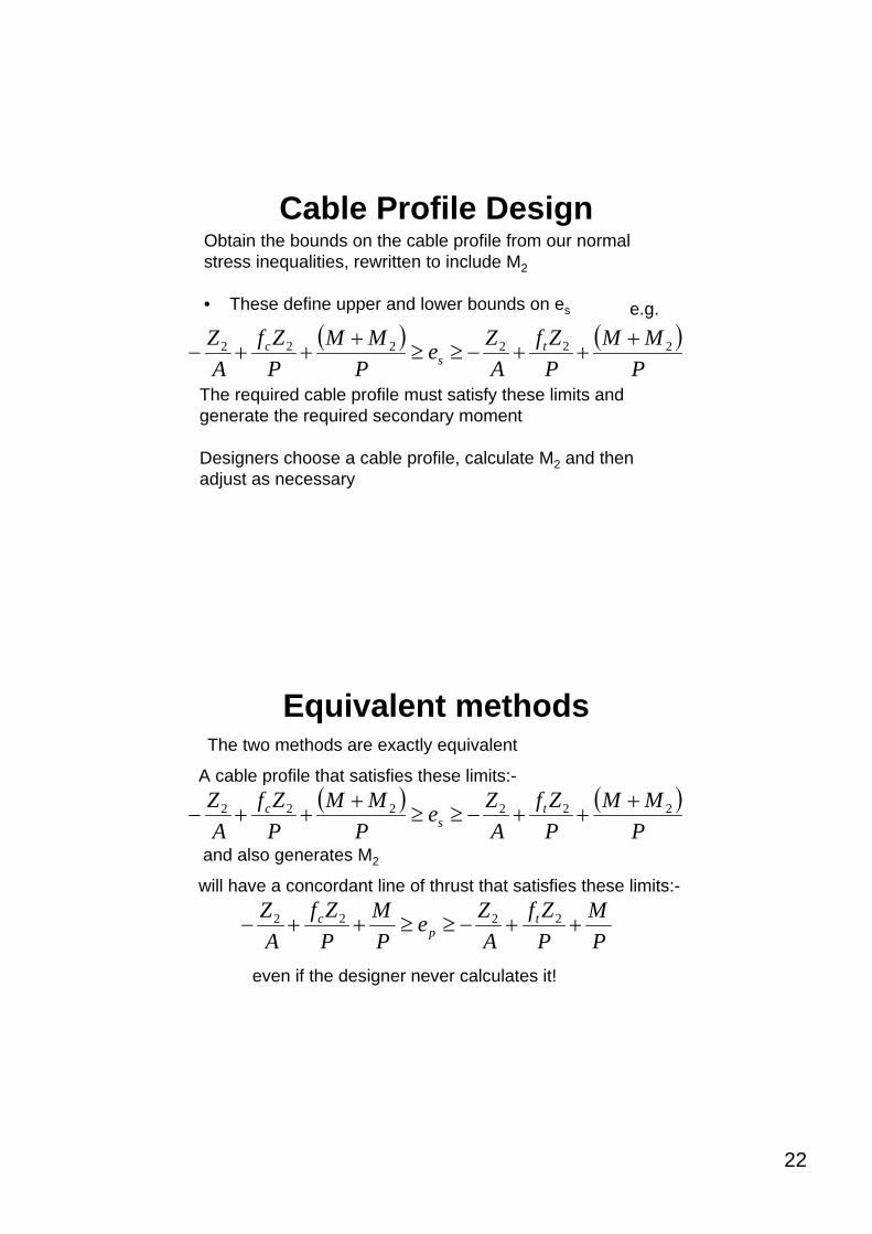
Cable Profile DesignObtain the bounds on the cable profile from our normal stress inequalities, rewritten to include M2

• These define upper and lower bounds on es

The required cable profile must satisfy these limits and generate the required secondary moment

Designers choose a cable profile, calculate M2 and then adjust as necessary

( ) ( )P

MMPZf

AZe

PMM

PZf

AZ t

sc 222222 +

++−≥≥+

++−

e.g.

Equivalent methodsThe two methods are exactly equivalent

( ) ( )P

MMPZf

AZe

PMM

PZf

AZ t

sc 222222 +

++−≥≥+

++−

A cable profile that satisfies these limits:-

and also generates M2

PM

PZf

AZe

PM

PZf

AZ t

pc ++−≥≥++− 2222

will have a concordant line of thrust that satisfies these limits:-

even if the designer never calculates it!

23

Logical design sequence1. Choose M2 required and add to effect of applied

loads2. Design section and choose prestress force3. Find limits on es

4. Use Linear transformation to find limits on ep

5. Find notional loads by automated method and hence ep

6. Transform back to get actual cable profile

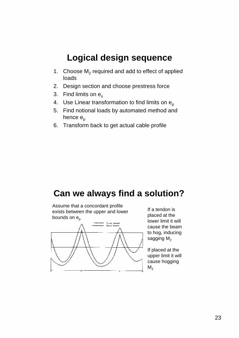
Can we always find a solution?Assume that a concordant profile exists between the upper and lower bounds on ep

If a tendon is placed at the lower limit it will cause the beam to hog, inducing sagging M2

If placed at the upper limit it will cause hogging M2

24

For a solution to exist • a cable placed at the upper limit must give

hogging M2, and• a cable placed at the lower limit must give a

sagging M2• For a particular value of P, the two limits can

be checked for this condition• Possible to produce expressions for the

limiting value of P

0.min =∫ dxEIPeiβ

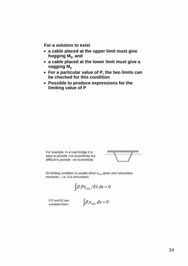
For example, in a road bridge it is easy to provide +ve eccentricity but difficult to provide –ve eccentricity.

So limiting condition is usually when emin gives zero secondary moments – i.e. it is concordant.

0.min =∫ dxeiβIf P and EI are constant then:-

25

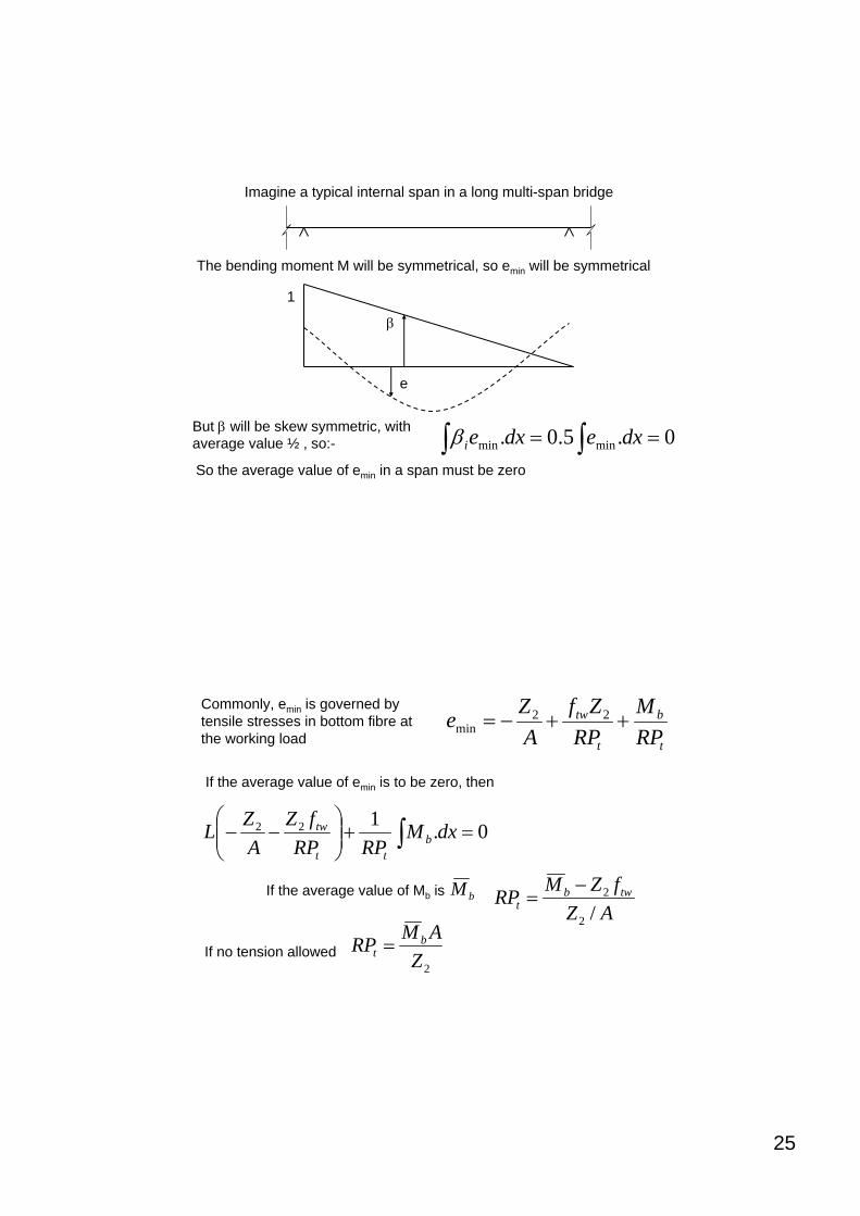
Imagine a typical internal span in a long multi-span bridge

e

The bending moment M will be symmetrical, so emin will be symmetrical

1

β

But β will be skew symmetric, with average value ½ , so:- 0.5.0. minmin == ∫∫ dxedxeiβSo the average value of emin in a span must be zero

t

b

t

tw

RPM

RPZf

AZe ++−= 22

min

Commonly, emin is governed by tensile stresses in bottom fibre at the working load

0.122 =+⎟⎟⎠

⎞⎜⎜⎝

⎛−− ∫ dxM

RPRPfZ

AZL b

tt

tw

If the average value of emin is to be zero, then

bMIf the average value of Mb is

AZfZMRP twb

t /2

2−=

If no tension allowed2ZAMRP b

t =

26

Easy to show that this is a minimum value for required P

Low called this value P3

(His P1 corresponds to our Pmin from the Magnel diagram and his P2is a value chosen to ensure that the cable fits within the section at both the mid-span region and over the piers)

If P < P3 it will be impossible to obtain a concordant line of thrust forthe cable no matter what adjustments are made to the profile.

N.B. Many assumptions made in this example but easy to rework if other conditions apply.

Ref. Low A M, The preliminary design of prestressed concrete viaducts, Procs ICE, 1982, 73, 351-364and Burgoyne C J, Cable design for continuous prestressed concrete bridges, Procs ICE, 1988, 85, 161-184

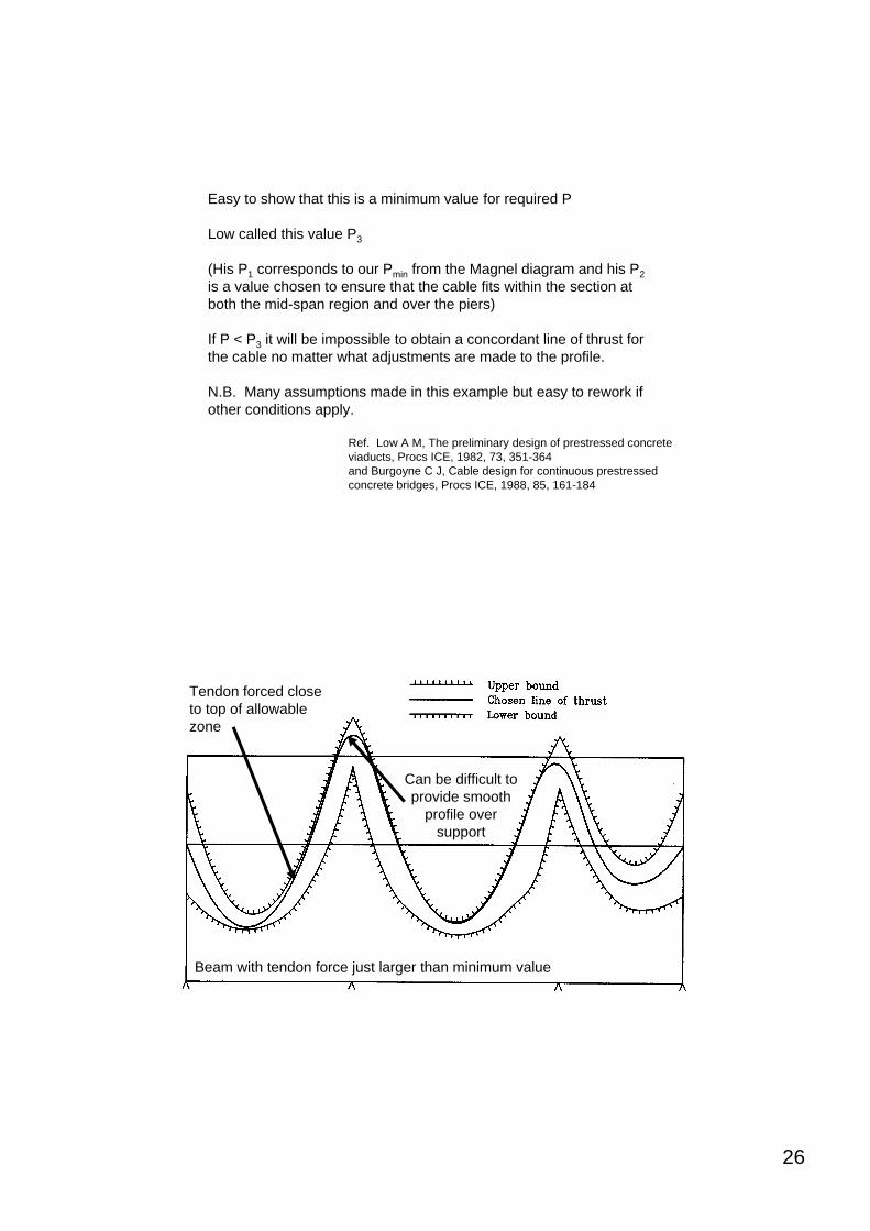
Beam with tendon force just larger than minimum value

Can be difficult to provide smooth

profile over support

Tendon forced close to top of allowable zone

27

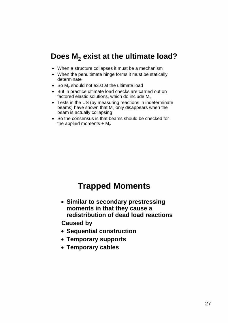
Does M2 exist at the ultimate load?• When a structure collapses it must be a mechanism• When the penultimate hinge forms it must be statically

determinate• So M2 should not exist at the ultimate load• But in practice ultimate load checks are carried out on

factored elastic solutions, which do include M2• Tests in the US (by measuring reactions in indeterminate

beams) have shown that M2 only disappears when the beam is actually collapsing

• So the consensus is that beams should be checked for the applied moments + M2

Trapped Moments

• Similar to secondary prestressing moments in that they cause a redistribution of dead load reactions

Caused by• Sequential construction• Temporary supports• Temporary cables

28

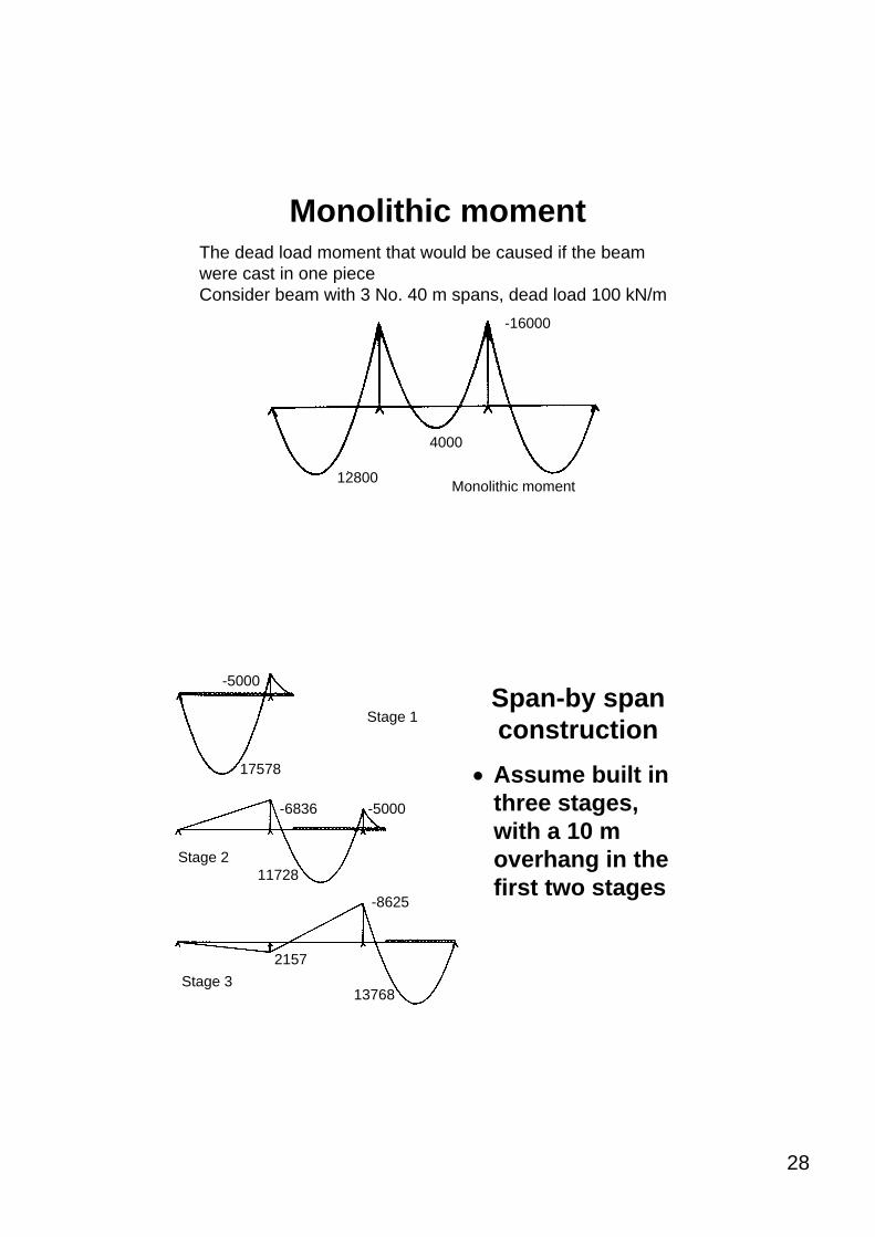
Monolithic momentThe dead load moment that would be caused if the beam were cast in one pieceConsider beam with 3 No. 40 m spans, dead load 100 kN/m

-16000

12800

4000

Monolithic moment

Span-by span construction

• Assume built in three stages, with a 10 m overhang in the first two stages

-5000

17578

Stage 1

-6836 -5000

11728Stage 2

2157

-8625

13768Stage 3

29

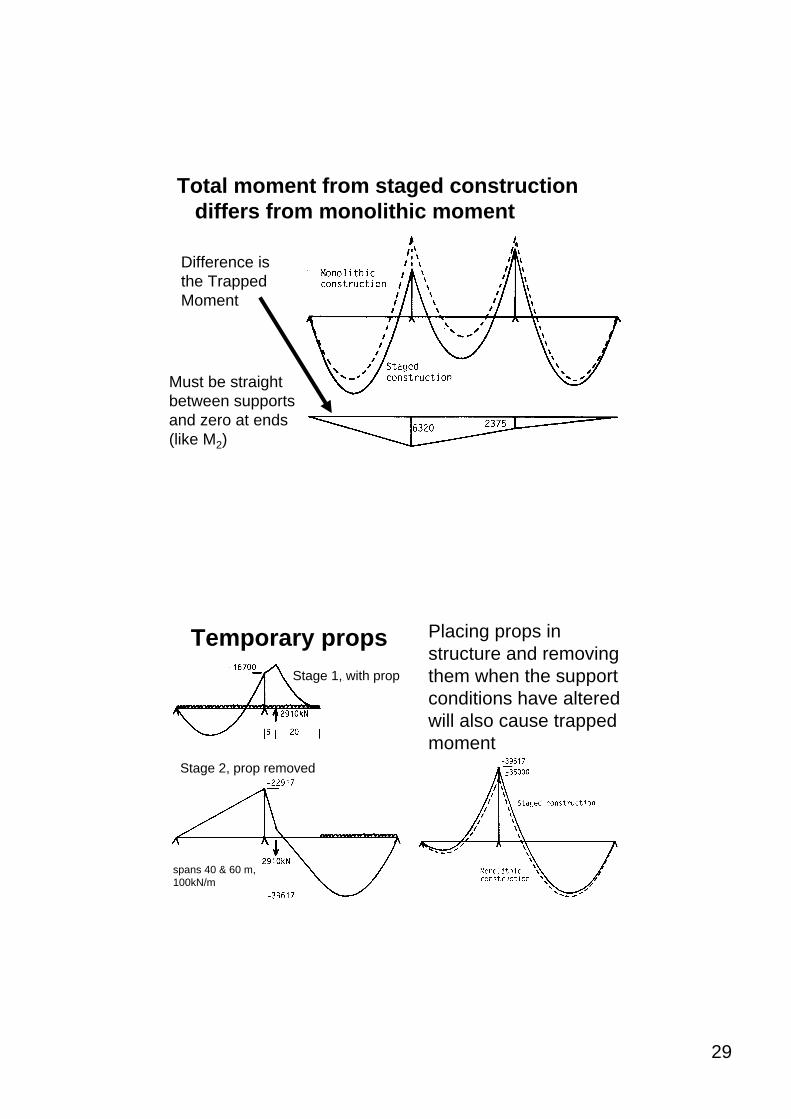
Total moment from staged construction differs from monolithic moment

Difference is the Trapped Moment

Must be straight between supports and zero at ends (like M2)

spans 40 & 60 m, 100kN/m

Temporary props Placing props in structure and removing them when the support conditions have altered will also cause trapped moment

Stage 1, with prop

Stage 2, prop removed

30

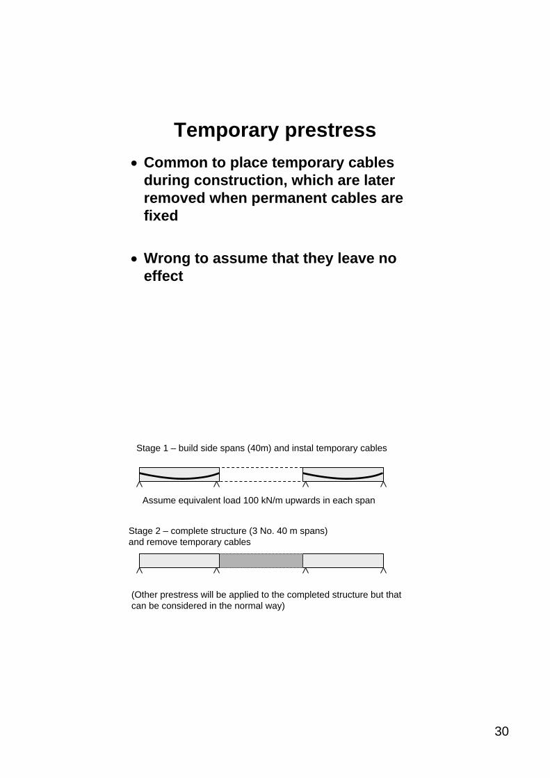
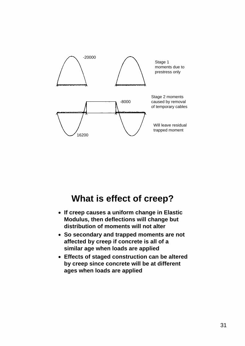
Temporary prestress• Common to place temporary cables

during construction, which are later removed when permanent cables are fixed

• Wrong to assume that they leave no effect

Stage 2 – complete structure (3 No. 40 m spans) and remove temporary cables

(Other prestress will be applied to the completed structure but that can be considered in the normal way)

Stage 1 – build side spans (40m) and instal temporary cables

Assume equivalent load 100 kN/m upwards in each span

31

Stage 1 moments due to prestress only

Stage 2 moments caused by removal of temporary cables

Will leave residual trapped moment

-20000

-8000

16200

What is effect of creep?• If creep causes a uniform change in Elastic

Modulus, then deflections will change but distribution of moments will not alter

• So secondary and trapped moments are not affected by creep if concrete is all of a similar age when loads are applied

• Effects of staged construction can be altered by creep since concrete will be at different ages when loads are applied