Module 5: Introduction to Multilevel Modelling SPSS … 5 (Practice): Intro to Multilevel Modelling Centre for Multilevel Modelling 2014 1 Module 5: Introduction to Multilevel Modelling

Module 5 (Practice): Intro to Multilevel Modelling

Centre for Multilevel Modelling 2014 1

Module 5: Introduction to Multilevel

Modelling SPSS Practicals Chris Charlton1

Centre for Multilevel Modelling

Pre-requisites

Modules 1-4

Contents

P5.1 Comparing Groups using Multilevel Modelling ........................................ 4

P5.1.1 A multilevel model of attainment with school effects ............................................................... 4 P5.1.2 Examining school effects (residuals)........................................................................................ 8

P5.2 Adding Student-level Explanatory Variables: Random Intercept Models ......... 14

P5.3 Allowing for Different Slopes across Schools: Random Slope Models ............. 19

P5.3.1 Testing for random slopes ...................................................................................................... 20 P5.3.2 Interpretation of random cohort effects across schools ......................................................... 21 P5.3.3 Examining intercept and slope residuals for schools ............................................................. 21 P5.3.4 Between-school variance as a function of cohort .................................................................. 25 P5.3.5 Adding a random coefficient for gender (dichotomous x ) ..................................................... 28 P5.3.6 Adding a random coefficient for social class (categorical x) ................................................. 30

P5.4 Adding Level 2 Explanatory Variables ................................................. 38

P5.4.1 Contextual effects ................................................................................................................... 42 P5.4.2 Cross-level interactions ......................................................................................................... 47

P5.5 Complex Level 1 Variation .............................................................. 51

P5.5.1 Within-school variance as a function of cohort (continuous X) ............................................. 51 P5.5.2 Within-school variance as a function of gender (dichotomous X) ......................................... 51 P5.5.3 Within-school variance as a function of cohort and gender .................................................. 55

P5.6 Appendices ................................................................................ 56

P5.6.1 Appendix 1 ............................................................................................................................. 56 P5.6.2 Appendix 2 ............................................................................................................................. 63

1 This SPSS practical is adapted from the corresponding MLwiN practical: Steele, F. (2008) Module 5: Introduction to Multilevel Modelling. LEMMA VLE, Centre for Multilevel Modelling. Accessed at http://www.cmm.bris.ac.uk/lemma/course/view.php?id=13.



Some of the sections within this module have online quizzes for you to test your understanding. To find the quizzes: EXAMPLE From within the LEMMA learning environment

Go down to the section for Module 5: Introduction to Multilevel Modelling

Click "5.1 Comparing Groups Using Multilevel Modelling" to open Lesson 5.1

Click Q 1 to open the first question

Introduction to the Scottish Youth Cohort Trends Dataset You will be analysing data from the Scottish School Leavers Survey (SSLS), a nationally representative survey of young people. We use data from seven cohorts of young people collected in the first sweep of the study, carried out at the end of the final year of compulsory schooling (aged 16-17) when most sample members had taken Standard grades2. In the practical for Module 3 on multiple regression, we considered the predictors of attainment in Standard grades (subject-based examinations, typically taken in up to eight subjects). In this practical, we extend the (previously single-level) multiple regression analysis to allow for dependency of exam scores within schools and to examine the extent of between-school variation in attainment. We also consider the effects on attainment of several school-level predictors. The dependent variable is a total attainment score. Each subject is graded on a scale from 1 (highest) to 7 (lowest) and, after recoding so that a high numeric value denotes a high grade, the total is taken across subjects. The analysis dataset contains the student-level variables considered in Module 3 together with a school identifier and three school-level variables:

Variable name Description and codes

CASEID Anonymised student identifier

SCHOOLID Anonymised school identifier

SCORE Point score calculated from awards in Standard grades taken at age 16. Scores range from 0 to 75, with a higher score indicating a higher attainment

COHORT90 The sample includes the following cohorts: 1984, 1986, 1988, 1990, 1996 and 1998. The

2 We are grateful to Linda Croxford (Centre for Educational Sociology, University of Edinburgh) for providing us with these data. The dataset was constructed as part of an ESRC-funded project on Education and Youth Transitions in England, Wales and Scotland 1984-2002. Further analyses of the data can be found in Croxford, L. and Raffe, D. (2006) Education Markets and Social Class Inequality: A Comparison of Trends in England, Scotland and Wales”. In R. Teese (Ed.) Inequality Revisited. Berlin: Springer.



COHORT90 variable is calculated by subtracting 1990 from each value. Thus values range from -6 (corresponding to 1984) to 8 (1998), with 1990 coded as zero

FEMALE Sex of student (1=female, 0=male)

SCLASS Social class, defined as the higher class of mother or father (1=managerial and professional, 2=intermediate, 3=working, 4=unclassified).

SCHTYPE School type, distinguishing independent schools from state-funded schools (1=independent, 0=state-funded)

SCHURBAN Urban-rural classification of school (1=urban, 0=town or rural)

SCHDENOM School denomination (1=Roman Catholic, 0=non-denominational)

There are 33988 students in 508 schools. Open the worksheet to From within the LEMMA Learning Environment

Go to Module 5: Introduction to Multilevel Modelling, and scroll down to SPSS Datafiles

Click “5.1.sav” You will see the Data Editor Window, after switching to Variable View:



P5.1 Comparing Groups using Multilevel Modelling

P5.1.1 A multilevel model of attainment with school effects We will start with the simplest multilevel model which allows for school effects on attainment, but without explanatory variables. This ‘null’ model may be written

(5.1)

where is the attainment of student i in school j , β0 is the overall mean across

schools, is the effect of school j on attainment, and is a student level

residual. The school effects , which we will also refer to as school (or level 2)

residuals, are assumed to follow a normal distribution with mean zero and

variance .

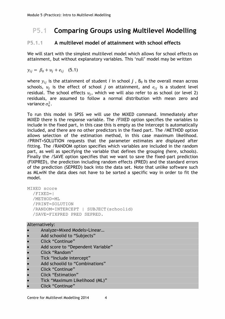
To run this model in SPSS we will use the MIXED command. Immediately after MIXED there is the response variable. The /FIXED option specifies the variables to include in the fixed part, in this case this is empty as the intercept is automatically included, and there are no other predictors in the fixed part. The /METHOD option allows selection of the estimation method, in this case maximum likelihood. /PRINT=SOLUTION requests that the parameter estimates are displayed after fitting. The /RANDOM option specifies which variables are included in the random part, as well as specifying the variable that defines the grouping (here, schools). Finally the /SAVE option specifies that we want to save the fixed-part prediction (FIXPRED), the prediction including random effects (PRED) and the standard errors of the prediction (SEPRED) back into the data set. Note that unlike software such as MLwiN the data does not have to be sorted a specific way in order to fit the model. MIXED score

/FIXED=|

/METHOD=ML

/PRINT=SOLUTION

/RANDOM=INTERCEPT | SUBJECT(schoolid)

/SAVE=FIXPRED PRED SEPRED.

Alternatively:

Analyze>Mixed Models>Linear…

Add schoolid to “Subjects”

Click “Continue”

Add score to “Dependent Variable”

Click “Random”

Tick “Include intercept”

Add schoolid to “Combinations”


Click “Estimation”

Tick “Maximum Likelihood (ML)”




Click “Statistics”

Tick “Parameter estimates”


Click “Save…”

Tick Predicted values under “Fixed Predicted Values”

Tick Predicted values under “Predicted Values & Residuals”

Tick Standard errors under “Predicted Values & Residuals”


Click “OK” We will see the following tables of results (the “Model Dimension” and “Type III Tests of Fixed Effects” tables are not of interest for this analysis, so we will omit them from subsequent results):

Model Dimensiona

Number of

Levels

Covariance

Structure

Number of

Parameters

Subject

Variables

Fixed Effects Intercept 1 1

Random Effects Intercept 1 Variance

Components

1 schoolid

Residual 1

Total 2 3

a. Dependent Variable: Score.

Information Criteriaa

-2 Log Likelihood 286539.064

Akaike's Information

Criterion (AIC)

286545.064

Hurvich and Tsai's Criterion

(AICC)

286545.065

Bozdogan's Criterion (CAIC) 286573.365

Schwarz's Bayesian

Criterion (BIC)

286570.365

The information criteria are displayed in

smaller-is-better forms.


Type III Tests of Fixed Effectsa

Source Numerator df Denominator df F Sig.



Intercept 1 451.533 6861.108 .000


Estimates of Fixed Effectsa

Parameter Estimate Std. Error df t Sig.

95% Confidence Interval

Lower Bound Upper Bound

Intercept 30.600595 .369430 451.533 82.832 .000 29.874579 31.326612


Estimates of Covariance Parametersa

Parameter Estimate Std. Error

Residual 258.357255 1.997715

Intercept [subject =

schoolid]

Variance 61.024127 4.475315


The overall mean attainment (across schools) is estimated as 30.60. The mean for

school j is estimated as 30.60 + ̂ , where ̂ is the school residual which we will

estimate in a moment. A school with ̂ > 0 has a mean that is higher than

average, while ̂ < 0 for a below-average school. (We will obtain confidence

intervals for residuals to determine whether differences from the overall mean can be considered ‘real’ or due to chance.) Partitioning variance

The between-school (level 2) variance in attainment is estimated as ̂ = 61.02,

and the within-school between-student (level 1) variance (labelled ‘Residual’ in

the output) is estimated as ̂ =258.36. Thus the total variance is

61.02+258.36=319.38. The variance partition coefficient (VPC) is 61.02/319.38 = 0.19, which indicates that 19% of the variance in attainment can be attributed to differences between schools. Note, however, that we have not accounted for intake ability (measured by exams taken on entry to secondary school) so the school effects are not value- added. Previous studies have found that between-school variance in progress, i.e. after accounting for intake attainment, is typically close to 10%. Testing for school effects

This document is only the first few pages of the full version. To see the complete document please go to learning materials and register: http://www.cmm.bris.ac.uk/lemma The course is completely free. We ask for a few details about yourself for our research purposes only. We will not give any details to any other organisation unless it is with your express permission.

http://www.cmm.bris.ac.uk/lemma

Documents

Module 5: Introduction to Multilevel Modelling SPSS … 5 (Practice): Intro to Multilevel Modelling Centre for Multilevel Modelling 2014 1 Module 5: Introduction to Multilevel Modelling