Embed Size (px)
Citation preview
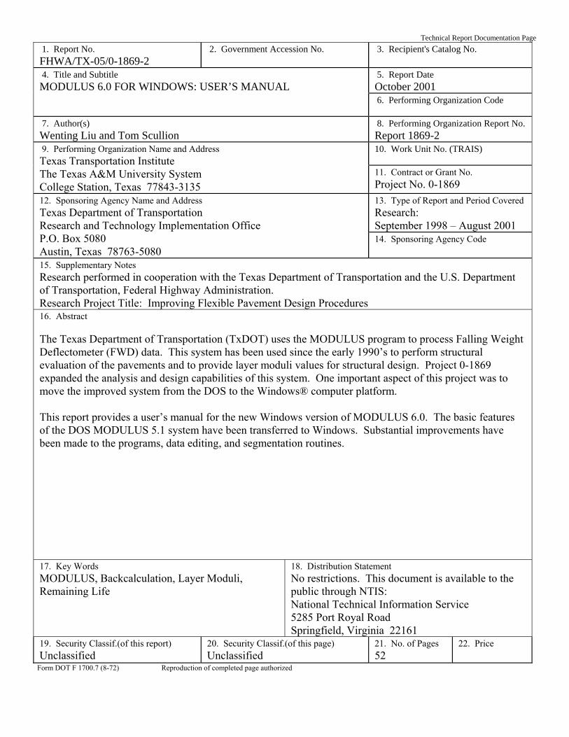
Technical Report Documentation Page 1. Report No. FHWA/TX-05/0-1869-2
2. Government Accession No.
3. Recipient's Catalog No. 5. Report Date October 2001
4. Title and Subtitle MODULUS 6.0 FOR WINDOWS: USER’S MANUAL
6. Performing Organization Code
7. Author(s) Wenting Liu and Tom Scullion
8. Performing Organization Report No. Report 1869-2 10. Work Unit No. (TRAIS)
9. Performing Organization Name and Address Texas Transportation Institute The Texas A&M University System College Station, Texas 77843-3135
11. Contract or Grant No. Project No. 0-1869 13. Type of Report and Period Covered Research: September 1998 – August 2001
12. Sponsoring Agency Name and Address Texas Department of Transportation Research and Technology Implementation Office P.O. Box 5080 Austin, Texas 78763-5080
14. Sponsoring Agency Code
15. Supplementary Notes Research performed in cooperation with the Texas Department of Transportation and the U.S. Department of Transportation, Federal Highway Administration. Research Project Title: Improving Flexible Pavement Design Procedures 16. Abstract The Texas Department of Transportation (TxDOT) uses the MODULUS program to process Falling Weight Deflectometer (FWD) data. This system has been used since the early 1990’s to perform structural evaluation of the pavements and to provide layer moduli values for structural design. Project 0-1869 expanded the analysis and design capabilities of this system. One important aspect of this project was to move the improved system from the DOS to the Windows® computer platform. This report provides a user’s manual for the new Windows version of MODULUS 6.0. The basic features of the DOS MODULUS 5.1 system have been transferred to Windows. Substantial improvements have been made to the programs, data editing, and segmentation routines. 17. Key Words MODULUS, Backcalculation, Layer Moduli, Remaining Life
18. Distribution Statement No restrictions. This document is available to the public through NTIS: National Technical Information Service 5285 Port Royal Road Springfield, Virginia 22161
19. Security Classif.(of this report) Unclassified
20. Security Classif.(of this page) Unclassified
21. No. of Pages 52
22. Price
Form DOT F 1700.7 (8-72) Reproduction of completed page authorized


MODULUS 6.0 FOR WINDOWS: USER’S MANUAL by
Wenting Liu Visiting Assistant Research Scientist
Texas Transportation Institute
and
Tom Scullion
Research Engineer Texas Transportation Institute
Report 0-1869-2 Project Number 0-1869 Research Project Title: Improving Flexible Pavement Design Procedures Sponsored by the Texas Department of Transportation
In Cooperation with the U.S. Department of Transportation Federal Highway Administration
October 2001 TEXAS TRANSPORTATION INSTITUTE The Texas A&M University System
College Station, Texas 77843-3135


v
DISCLAIMER
The contents of this report reflect the views of the authors, who are responsible for the
facts and the accuracy of the data presented herein. The contents do not necessarily reflect the
official view or policies of the Federal Highway Administration (FHWA) or the Texas
Department of Transportation (TxDOT). This report does not constitute a standard,
specification, or regulation. The engineer in charge was Tom Scullion, P.E. #62683.

vi
ACKNOWLEDGMENTS
Mark McDaniel was the project director on this project. His support, encouragement and
patience are greatly appreciated. This project was sponsored by TxDOT’s Research
Management Committee (RMC 1) for Pavements and Design. Elias Rmeili PE., Andrew
Wimsatt PE., Joe Leidy PE and Darlene Goehl PE actively participated in the development of
these new analysis tools.
vii
TABLE OF CONTENTS
Page
List of Figures .............................................................................................................................. viii
Chapter 1. Introduction ...................................................................................................................1
1.1 Differences Between Modulus 6.0 for Windows and Earlier Versions of Modulus ....1
1.2 System Requirements....................................................................................................2
1.3 Getting Started ..............................................................................................................2
Chapter 2. Main Menu Screen ........................................................................................................3
Chapter 3. Pre-Processing...............................................................................................................5
3.1 Read FWD Data............................................................................................................5
3.2 Drop Select Routine......................................................................................................8
3.3 Station Select Routine.................................................................................................10
Chapter 4. Remaining Life Routine ..............................................................................................15
Chapter 5. MODULUS Backcalculation Routine.........................................................................19
Chapter 6. Segmentation...............................................................................................................29
Chapter 7. Postprocessing Graphing Routines .............................................................................33
References......................................................................................................................................41
viii
LIST OF FIGURES
Figure Page
1. Main Menu Screen for MODULUS for Windows. ............................................................ 3
2. Open a FWD Test File. ....................................................................................................... 5
3. Comment File Display. ....................................................................................................... 6
4. Inputting Non-Standard Data Files. .................................................................................... 7
5. FWD Drop Select Screen.................................................................................................... 8
6. Drop Selection with the Text Box .................................................................................... 10
7. Depth to Bedrock Analysis Input Window....................................................................... 10
8. Selecting Bowls to be Dropped from Analysis................................................................. 12
9. Station Selection by the Chart. ......................................................................................... 13
10. Comment View by Clicking the Pink Circle. ................................................................... 14
11. Remaining Life Analysis Input Dialogue Box. ................................................................ 15
12. View the FWD Measured Temperature. ........................................................................... 16
13. Remaining Life Result Chart. ........................................................................................... 17
14. MODULUS Backcalculation Input Dialogue Box. .......................................................... 19
15. Semi-Infinite Subgrade Model.......................................................................................... 20
16. View the FWD Measured Temperature. ........................................................................... 21
17. BackCalculation Result Chart........................................................................................... 22
18. View Backcalculation Result File..................................................................................... 23
19. Get the Value of Each Point. ............................................................................................ 24
20. View the Detail Tested and Calculated Deflection........................................................... 25
21. Select a Station for Manual Backcalculation Analysis..................................................... 26
22. Manual Backcalculation Screen........................................................................................ 26
23. Using the Manual Backcalculation. .................................................................................. 27
24. Data Segmentation Analysis. ............................................................................................ 29
25. Automatic Segmentation Result Display. ......................................................................... 30
26. Manually Add or Remove Segment and Segment Table Display. ................................... 31
ix
27. View Segmentation Output File. ...................................................................................... 31
28. Print Chart Control Screen................................................................................................ 33
29. View and Print the Layer Strength ................................................................................... 34
30. View and Print the Remaining Life .................................................................................. 35
31. Chart Display on Screen. .................................................................................................. 35
32. Title Option Screen. .......................................................................................................... 36
33. Axis Scale Control Screen. ............................................................................................... 37
34. Axis Font Control Screen. ................................................................................................ 37
35. Axis Number Decimal Control Screen. ............................................................................ 38
36. Chart Line Pattern Control Screen.................................................................................... 38
37. Chart Legend Control Screen. .......................................................................................... 39
38. Chart Gridline Control Screen. ......................................................................................... 39

1
CHAPTER 1. INTRODUCTION
1.1 DIFFERENCES BETWEEN MODULUS 6.0 FOR WINDOWS AND EARLIER
VERSIONS OF MODULUS
For those users who are familiar with an earlier DOS version of MODULUS(5.1), the
following are the changes and new features that have been added to create version 6.0.
• Total Windows program which can run under Win-9*, Win-NT and Win-2000
• New segmentation algorithm was added which can automatically do the segmentation
work.
• A new manual segmentation has also been added.
• Supports most of the Dynatest FWD test file format including as R80 and R32.
• Supports a user data input function, this function lets the user input ASCII formatted
FWD data.
• A manual function has been added which permits the user to do the backcalculation
manually. The propose of this function is:
(1) To do a detailed analysis at one station (if the automated results are not satisfactory)
(2) Find the suitable moduli range for the layer thickness
• Improved selection criteria to select which FWD drop or station to process.
• Calculating the depth to bedrock for the entire data set before selecting the FWD data to
process. This function can let the user select the homogeneous depth to bedrock stations
to improve the moduli backcalculation result.
• A Graphic User Interface has been added.
• HTML-based help system is supported in this program. The F1 function key can access
the help system.
1.2 SYSTEM REQUIREMENTS
The minimum system requirements to run the program are:
• Operation systems: Windows 95/98/ME/NT 4.0/2000/XP
• CPU: Pentium-133 MHz or higher

2
• 16 MB RAM or higher
• 15 MB free hard drive space
• SVGA - True Color video mode
• For best running propose, the 1024×768 pixels screen resolution is recommended
• CD-ROM drive (if installation is done from a CD-ROM)
• Mouse or other suitable pointing device
• A printer supported by the computer running the program
1.3 GETTING STARTED
Version 6.0 of the TTI MODULUS backcalculation and remaining life analysis program is
furnished on a CD-R compact disk. Program files and the sample data files are installed to the
appropriate directories by running the setup program MODULUSsetup.exe on this CD.
Before installation, make sure that your computer meets the minimum requirements, and it is
strongly recommended that before proceeding, you ensure that no other Windows programs are
running.
Insert the program compact disc in the CD-ROM drive. Use the appropriate command in
your operating environment to run the setup program (MODULUSsetup.exe), which is available in
the root directory on the compact disc. Follow the setup instructions on the screen. The user can
change the default installation directory C:\Modwin. Once you have completed the setup procedure,
you can start running the MODULUS by using the desktop shortcut or the start button on the task
bar in Windows.
The setup program will install the following type files in your computer:
• DLL, OCX system files to the Windows system folder
• Execute program file “Modulus.exe”.
• Sample data file
A full user’s manual for MODULUS 6.0 is given is Chapter 2 of this report.
3
CHAPTER 2. MAIN MENU SCREEN
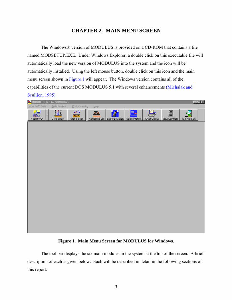
The Windows® version of MODULUS is provided on a CD-ROM that contains a file
named MODSETUP.EXE. Under Windows Explorer, a double click on this executable file will
automatically load the new version of MODULUS into the system and the icon will be
automatically installed. Using the left mouse button, double click on this icon and the main
menu screen shown in Figure 1 will appear. The Windows version contains all of the
capabilities of the current DOS MODULUS 5.1 with several enhancements (Michalak and
Scullion, 1995).
Figure 1. Main Menu Screen for MODULUS for Windows.
The tool bar displays the six main modules in the system at the top of the screen. A brief
description of each is given below. Each will be described in detail in the following sections of
this report.
4
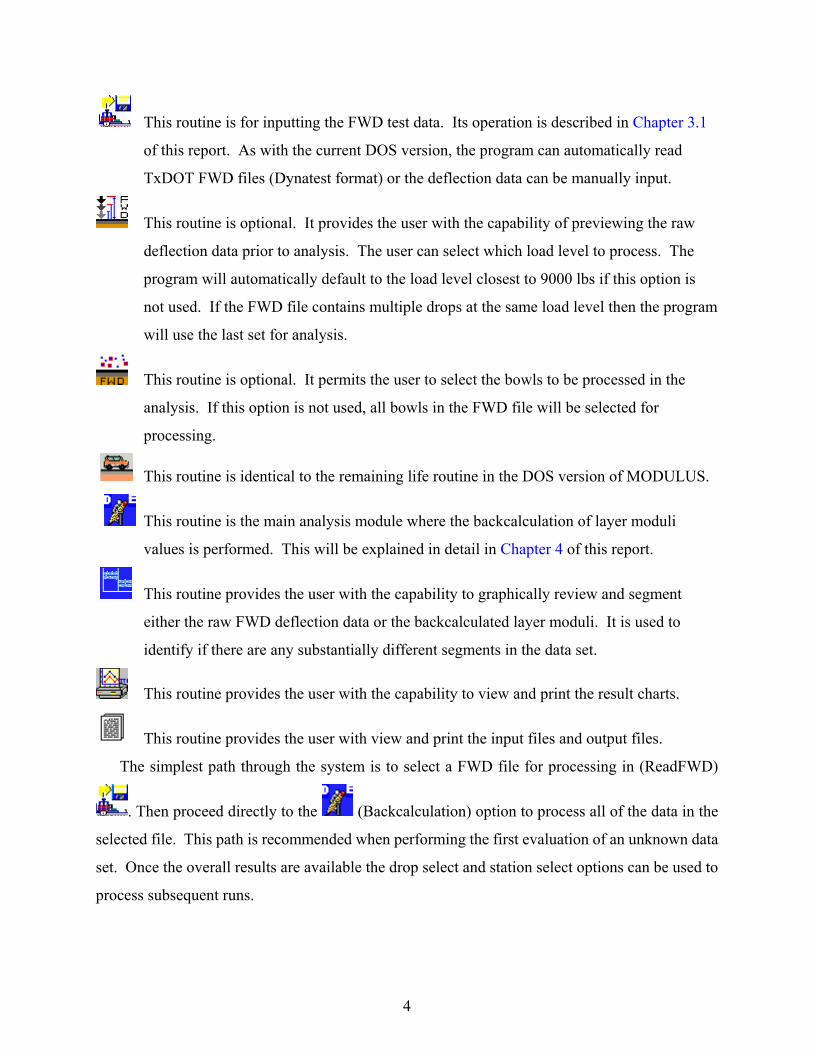
This routine is for inputting the FWD test data. Its operation is described in Chapter 3.1
of this report. As with the current DOS version, the program can automatically read
TxDOT FWD files (Dynatest format) or the deflection data can be manually input.
This routine is optional. It provides the user with the capability of previewing the raw
deflection data prior to analysis. The user can select which load level to process. The
program will automatically default to the load level closest to 9000 lbs if this option is
not used. If the FWD file contains multiple drops at the same load level then the program
will use the last set for analysis.
This routine is optional. It permits the user to select the bowls to be processed in the
analysis. If this option is not used, all bowls in the FWD file will be selected for
processing.
This routine is identical to the remaining life routine in the DOS version of MODULUS.
This routine is the main analysis module where the backcalculation of layer moduli
values is performed. This will be explained in detail in Chapter 4 of this report.
This routine provides the user with the capability to graphically review and segment
either the raw FWD deflection data or the backcalculated layer moduli. It is used to
identify if there are any substantially different segments in the data set.
This routine provides the user with the capability to view and print the result charts.
This routine provides the user with view and print the input files and output files.
The simplest path through the system is to select a FWD file for processing in (ReadFWD)
. Then proceed directly to the (Backcalculation) option to process all of the data in the
selected file. This path is recommended when performing the first evaluation of an unknown data
set. Once the overall results are available the drop select and station select options can be used to
process subsequent runs.

5
CHAPTER 3. PRE-PROCESSING
3.1 READ FWD DATA
This routine permits the user to read TxDOT’s standard FWD data files. It is activated
by a single click of the left mouse button on the ReadFWD icon .
Figure 2. Open a FWD Test File.
The program can read Dynatest FWD format R80, and R32 with format versions F9, F10,
and F20. This new system can also directly read FWD data files which contain dynamic time
history data. The dynamic data are not used in the analysis; only the deflection peaks are
extracted and processed.
The user selects the FWD file of interest with a single click of the left button, then opens
the file by clicking the Open button. (Double-clicking on the selected file will automatically
open the file.) The program then displays the comment file shown in Figure 3.
6
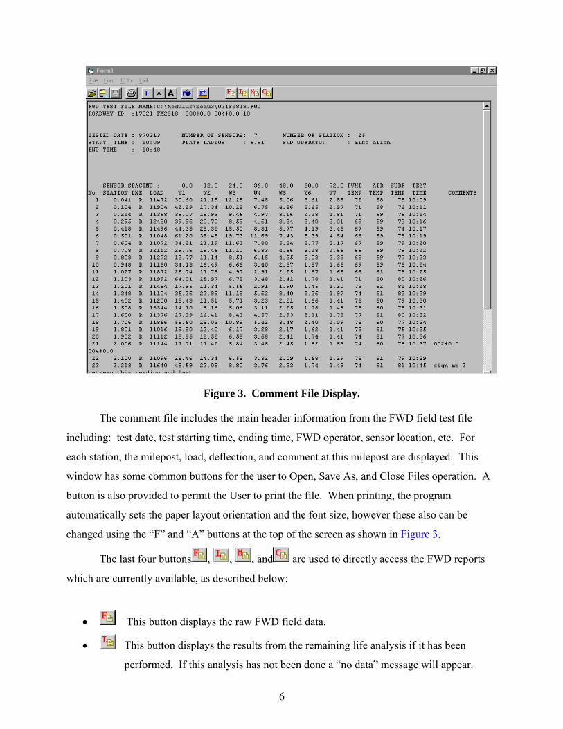
Figure 3. Comment File Display.
The comment file includes the main header information from the FWD field test file
including: test date, test starting time, ending time, FWD operator, sensor location, etc. For
each station, the milepost, load, deflection, and comment at this milepost are displayed. This
window has some common buttons for the user to Open, Save As, and Close Files operation. A
button is also provided to permit the User to print the file. When printing, the program
automatically sets the paper layout orientation and the font size, however these also can be
changed using the “F” and “A” buttons at the top of the screen as shown in Figure 3.
The last four buttons , , , and are used to directly access the FWD reports
which are currently available, as described below:
• This button displays the raw FWD field data.
• This button displays the results from the remaining life analysis if it has been
performed. If this analysis has not been done a “no data” message will appear.
7
• This button displays the standard results from the backcalculation analysis, if
available.
• This button displays the data in the comment file.
To return to the main menu screen, the arrow key in the header of the screen as
shown in Figure 3 is used.
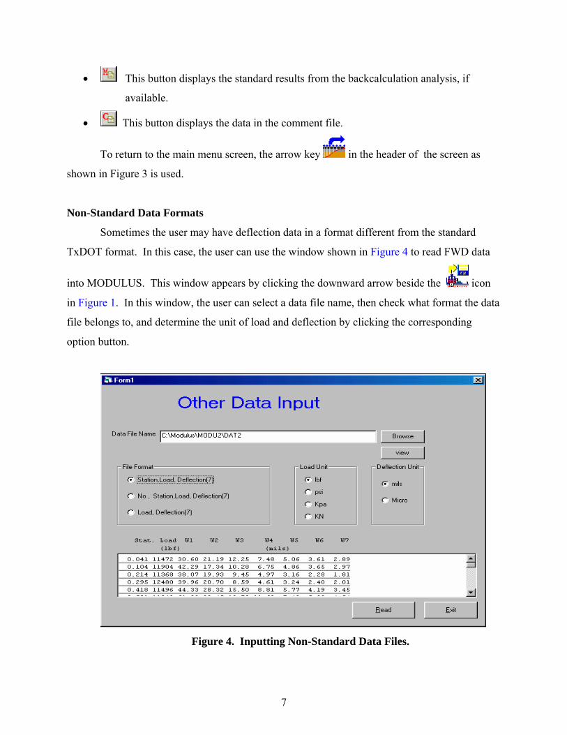
Non-Standard Data Formats
Sometimes the user may have deflection data in a format different from the standard
TxDOT format. In this case, the user can use the window shown in Figure 4 to read FWD data
into MODULUS. This window appears by clicking the downward arrow beside the icon
in Figure 1. In this window, the user can select a data file name, then check what format the data
file belongs to, and determine the unit of load and deflection by clicking the corresponding
option button.
Figure 4. Inputting Non-Standard Data Files.
8
The data file is supposed to be delimited by spaces (one or more spaces) or the tab key.
The bottom box shows the data, title and unit for the user to check if the user read the data
correctly. The Browse button is used to select another file. The View button can let the user
view this file with the same screen as in Figure 3.
If the user does not want to read the data, the user may press the Exit button to exit this
window. Clicking the Read button will let the program read the non-standard data and then
return to the main menu (Figure 1).
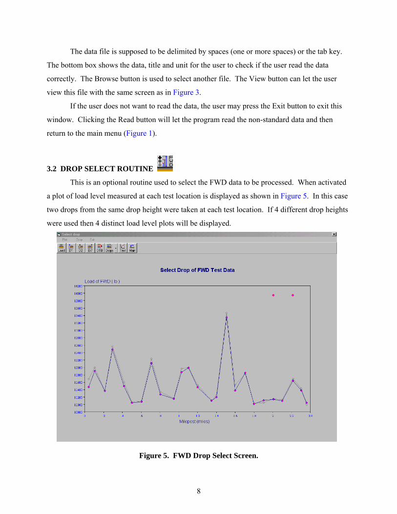
3.2 DROP SELECT ROUTINE
This is an optional routine used to select the FWD data to be processed. When activated
a plot of load level measured at each test location is displayed as shown in Figure 5. In this case
two drops from the same drop height were taken at each test location. If 4 different drop heights
were used then 4 distinct load level plots will be displayed.
Figure 5. FWD Drop Select Screen.
9
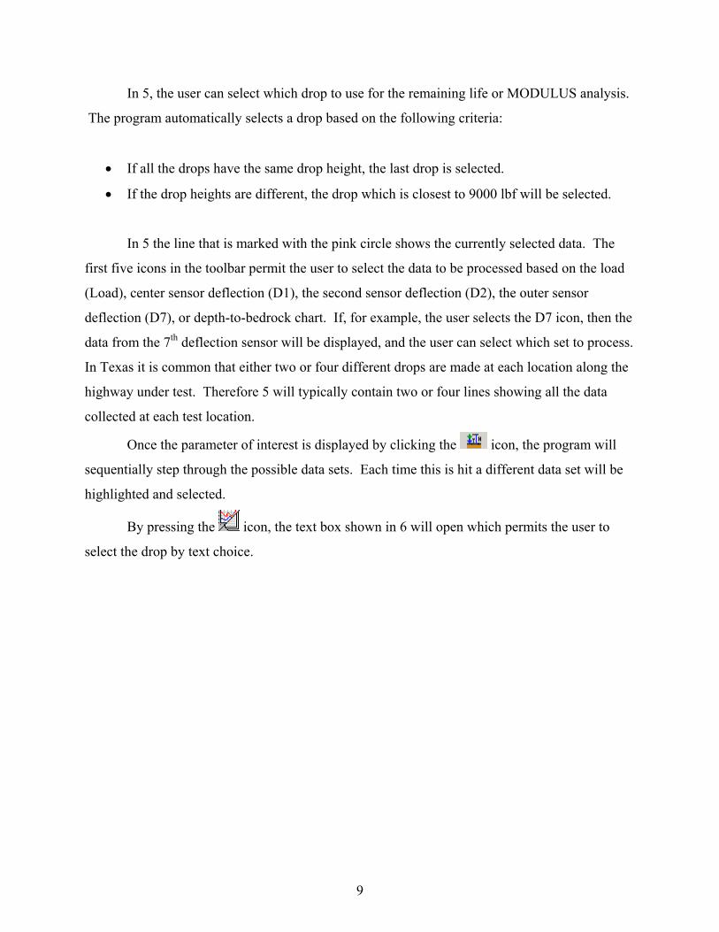
In 5, the user can select which drop to use for the remaining life or MODULUS analysis.
The program automatically selects a drop based on the following criteria:
• If all the drops have the same drop height, the last drop is selected.
• If the drop heights are different, the drop which is closest to 9000 lbf will be selected.
In 5 the line that is marked with the pink circle shows the currently selected data. The
first five icons in the toolbar permit the user to select the data to be processed based on the load
(Load), center sensor deflection (D1), the second sensor deflection (D2), the outer sensor
deflection (D7), or depth-to-bedrock chart. If, for example, the user selects the D7 icon, then the
data from the 7th deflection sensor will be displayed, and the user can select which set to process.
In Texas it is common that either two or four different drops are made at each location along the
highway under test. Therefore 5 will typically contain two or four lines showing all the data
collected at each test location.
Once the parameter of interest is displayed by clicking the icon, the program will
sequentially step through the possible data sets. Each time this is hit a different data set will be
highlighted and selected.
By pressing the icon, the text box shown in 6 will open which permits the user to
select the drop by text choice.
10
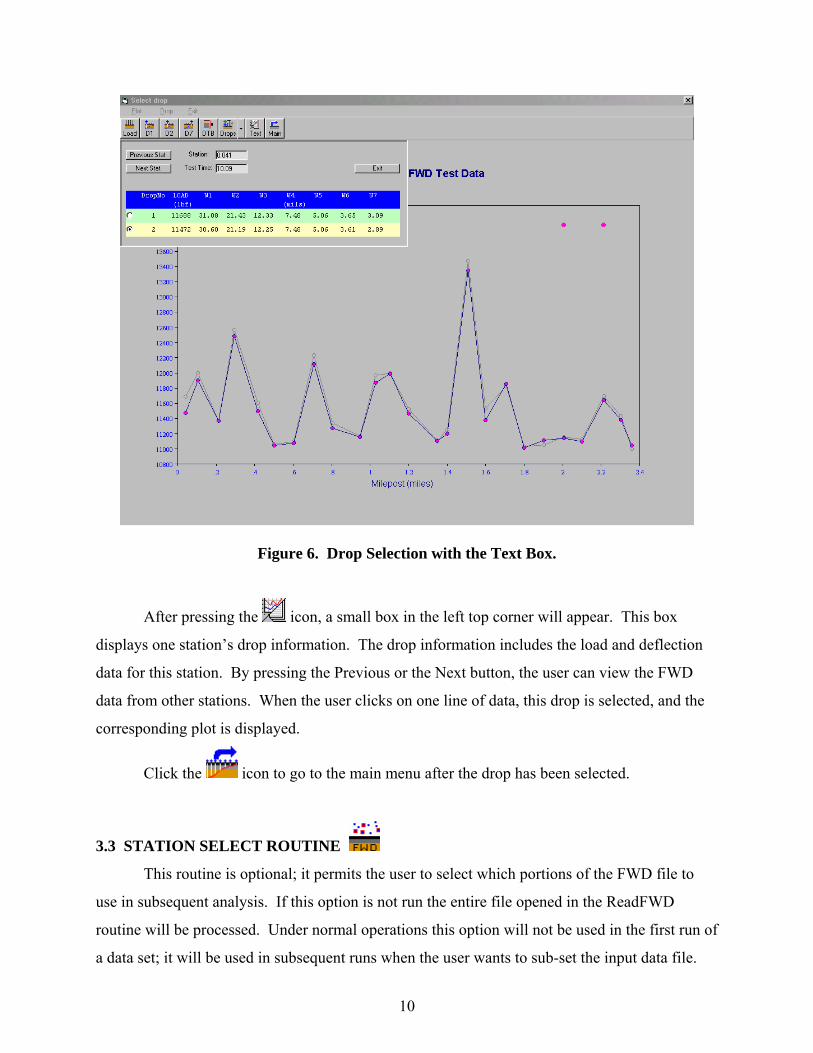
Figure 6. Drop Selection with the Text Box.
After pressing the icon, a small box in the left top corner will appear. This box
displays one station’s drop information. The drop information includes the load and deflection
data for this station. By pressing the Previous or the Next button, the user can view the FWD
data from other stations. When the user clicks on one line of data, this drop is selected, and the
corresponding plot is displayed.
Click the icon to go to the main menu after the drop has been selected.
3.3 STATION SELECT ROUTINE
This routine is optional; it permits the user to select which portions of the FWD file to
use in subsequent analysis. If this option is not run the entire file opened in the ReadFWD
routine will be processed. Under normal operations this option will not be used in the first run of
a data set; it will be used in subsequent runs when the user wants to sub-set the input data file.
11
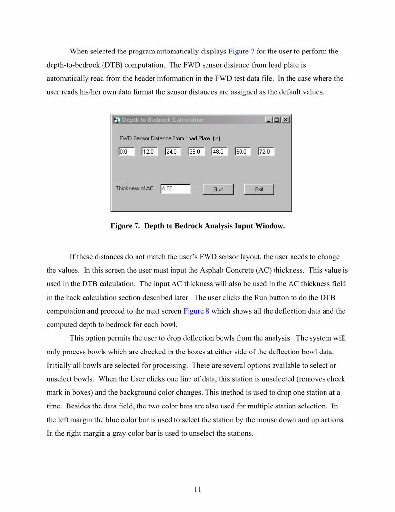
When selected the program automatically displays Figure 7 for the user to perform the
depth-to-bedrock (DTB) computation. The FWD sensor distance from load plate is
automatically read from the header information in the FWD test data file. In the case where the
user reads his/her own data format the sensor distances are assigned as the default values.
Figure 7. Depth to Bedrock Analysis Input Window.
If these distances do not match the user’s FWD sensor layout, the user needs to change
the values. In this screen the user must input the Asphalt Concrete (AC) thickness. This value is
used in the DTB calculation. The input AC thickness will also be used in the AC thickness field
in the back calculation section described later. The user clicks the Run button to do the DTB
computation and proceed to the next screen Figure 8 which shows all the deflection data and the
computed depth to bedrock for each bowl.
This option permits the user to drop deflection bowls from the analysis. The system will
only process bowls which are checked in the boxes at either side of the deflection bowl data.
Initially all bowls are selected for processing. There are several options available to select or
unselect bowls. When the User clicks one line of data, this station is unselected (removes check
mark in boxes) and the background color changes. This method is used to drop one station at a
time. Besides the data field, the two color bars are also used for multiple station selection. In
the left margin the blue color bar is used to select the station by the mouse down and up actions.
In the right margin a gray color bar is used to unselect the stations.
12
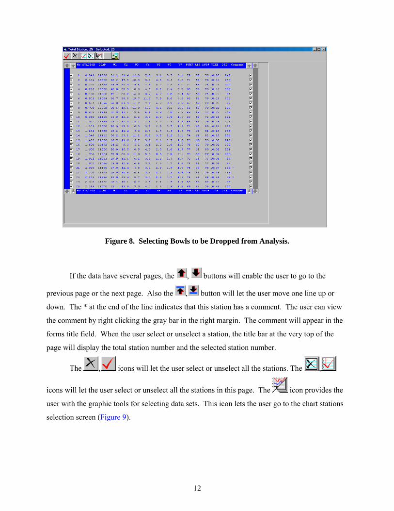
Figure 8. Selecting Bowls to be Dropped from Analysis.
If the data have several pages, the , buttons will enable the user to go to the
previous page or the next page. Also the , button will let the user move one line up or
down. The * at the end of the line indicates that this station has a comment. The user can view
the comment by right clicking the gray bar in the right margin. The comment will appear in the
forms title field. When the user select or unselect a station, the title bar at the very top of the
page will display the total station number and the selected station number.
The , icons will let the user select or unselect all the stations. The ,
icons will let the user select or unselect all the stations in this page. The icon provides the
user with the graphic tools for selecting data sets. This icon lets the user go to the chart stations
selection screen (Figure 9).
13
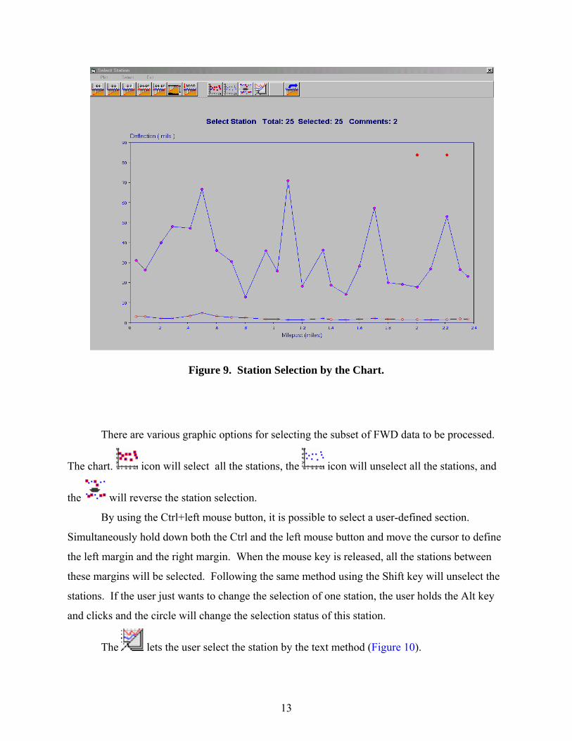
Figure 9. Station Selection by the Chart.
There are various graphic options for selecting the subset of FWD data to be processed.
The chart. icon will select all the stations, the icon will unselect all the stations, and
the will reverse the station selection.
By using the Ctrl+left mouse button, it is possible to select a user-defined section.
Simultaneously hold down both the Ctrl and the left mouse button and move the cursor to define
the left margin and the right margin. When the mouse key is released, all the stations between
these margins will be selected. Following the same method using the Shift key will unselect the
stations. If the user just wants to change the selection of one station, the user holds the Alt key
and clicks and the circle will change the selection status of this station.
The lets the user select the station by the text method (Figure 10).
14
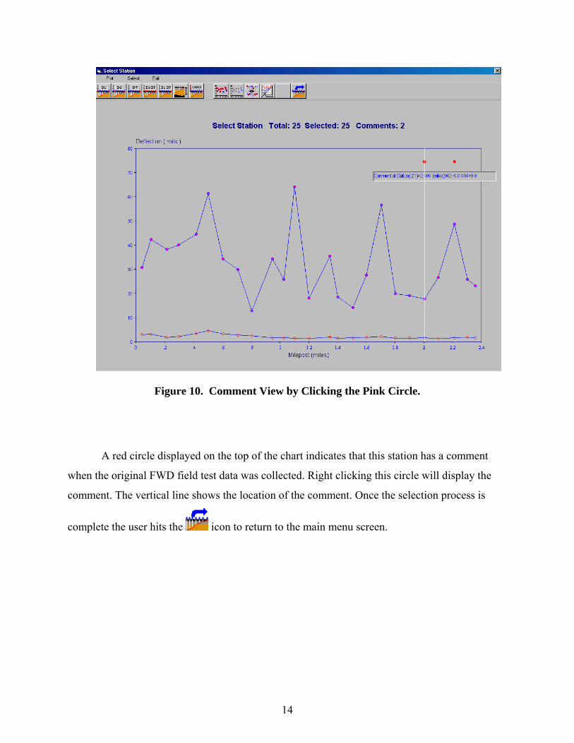
Figure 10. Comment View by Clicking the Pink Circle.
A red circle displayed on the top of the chart indicates that this station has a comment
when the original FWD field test data was collected. Right clicking this circle will display the
comment. The vertical line shows the location of the comment. Once the selection process is
complete the user hits the icon to return to the main menu screen.
15
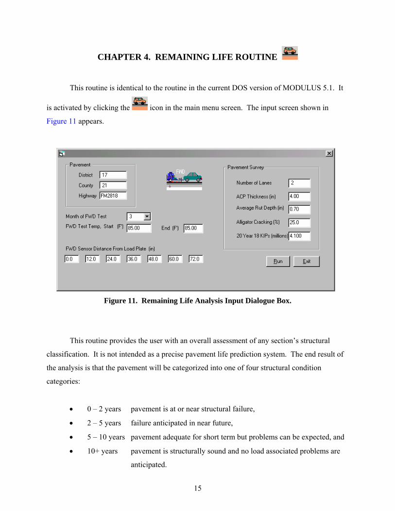
CHAPTER 4. REMAINING LIFE ROUTINE
This routine is identical to the routine in the current DOS version of MODULUS 5.1. It
is activated by clicking the icon in the main menu screen. The input screen shown in
Figure 11 appears.
Figure 11. Remaining Life Analysis Input Dialogue Box.
This routine provides the user with an overall assessment of any section’s structural
classification. It is not intended as a precise pavement life prediction system. The end result of
the analysis is that the pavement will be categorized into one of four structural condition
categories:
• 0 – 2 years pavement is at or near structural failure,
• 2 – 5 years failure anticipated in near future,
• 5 – 10 years pavement adequate for short term but problems can be expected, and
• 10+ years pavement is structurally sound and no load associated problems are
anticipated.
16
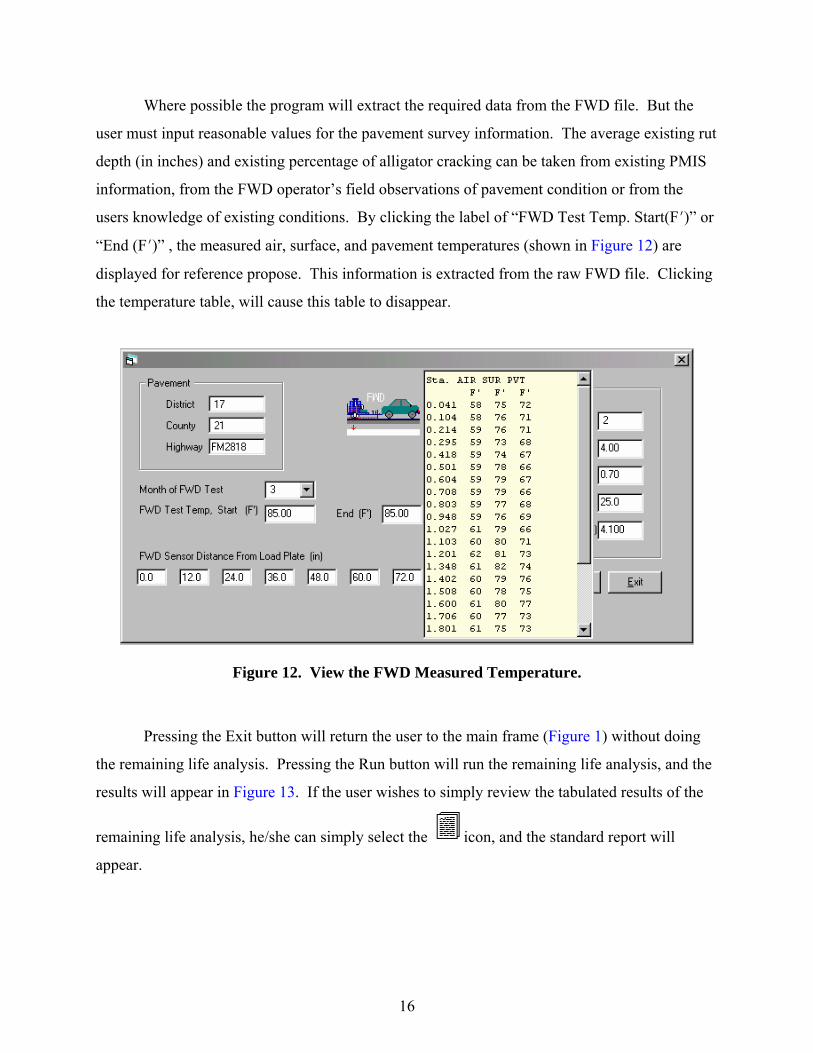
Where possible the program will extract the required data from the FWD file. But the
user must input reasonable values for the pavement survey information. The average existing rut
depth (in inches) and existing percentage of alligator cracking can be taken from existing PMIS
information, from the FWD operator’s field observations of pavement condition or from the
users knowledge of existing conditions. By clicking the label of “FWD Test Temp. Start(FN)” or
“End (FN)” , the measured air, surface, and pavement temperatures (shown in Figure 12) are
displayed for reference propose. This information is extracted from the raw FWD file. Clicking
the temperature table, will cause this table to disappear.
Figure 12. View the FWD Measured Temperature.
Pressing the Exit button will return the user to the main frame (Figure 1) without doing
the remaining life analysis. Pressing the Run button will run the remaining life analysis, and the
results will appear in Figure 13. If the user wishes to simply review the tabulated results of the
remaining life analysis, he/she can simply select the icon, and the standard report will
appear.
17
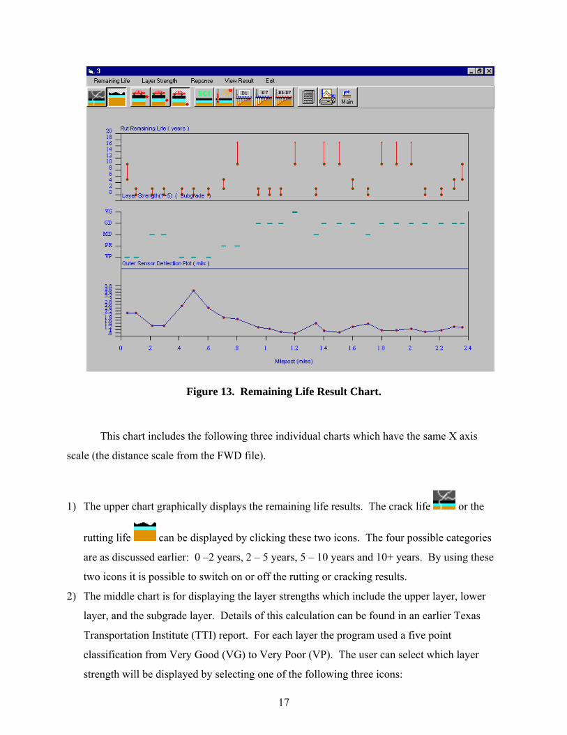
Figure 13. Remaining Life Result Chart.
This chart includes the following three individual charts which have the same X axis
scale (the distance scale from the FWD file).
1) The upper chart graphically displays the remaining life results. The crack life or the
rutting life can be displayed by clicking these two icons. The four possible categories
are as discussed earlier: 0 –2 years, 2 – 5 years, 5 – 10 years and 10+ years. By using these
two icons it is possible to switch on or off the rutting or cracking results.
2) The middle chart is for displaying the layer strengths which include the upper layer, lower
layer, and the subgrade layer. Details of this calculation can be found in an earlier Texas
Transportation Institute (TTI) report. For each layer the program used a five point
classification from Very Good (VG) to Very Poor (VP). The user can select which layer
strength will be displayed by selecting one of the following three icons:
18
This icon activates the strength assessment of the upper eight inches of the pavement
structure, based on the normalized surface curvature index (SCI) and the surface
thickness.
This provides an assessment of the layer strengths for 8 to 16 inches below the surface.
It is based on the normalized base curvature index.
This provides an assessment of the subgrade stiffness based on the deflections measured
at the outer FWD sensors.
3) The lower chart will display the surface curvature index (W1 – W2), raw deflections, or
measured temperature as selected using the available icons in the control bar at the top of the
screen (five icons in total).
The benefit of using these three charts in one screen is that the user can get a
comprehensive overview of the results and determines if substantially different structural
conditions exist along the highway.
The icon lets the user access the remaining life result file for viewing and printing. The
display and print options are identical to those discussed earlier.
19
CHAPTER 5. MODULUS BACKCALCULATION ROUTINE
This is the main computation model with MODULUS. The user activates it by selecting
the icon from the main screen, which will display the screen shown in Figure 14.
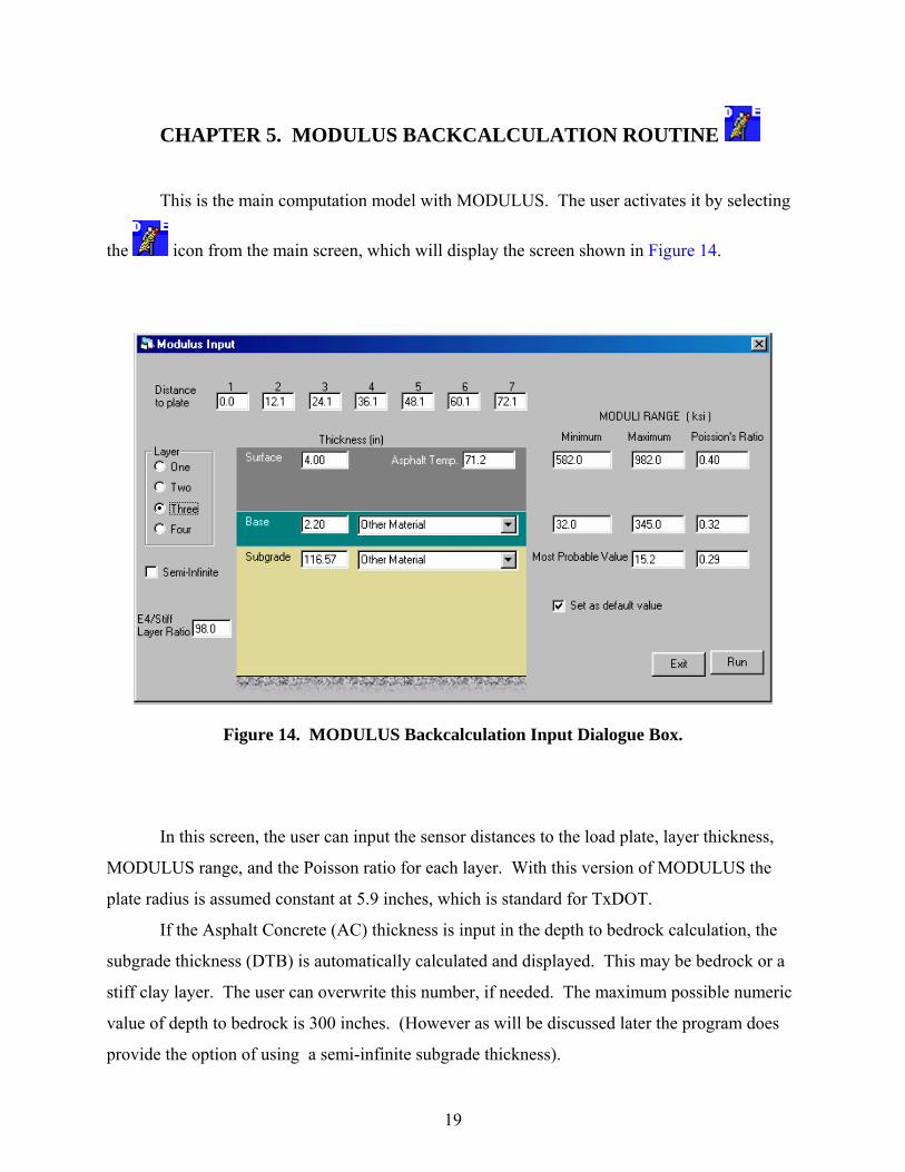
Figure 14. MODULUS Backcalculation Input Dialogue Box.
In this screen, the user can input the sensor distances to the load plate, layer thickness,
MODULUS range, and the Poisson ratio for each layer. With this version of MODULUS the
plate radius is assumed constant at 5.9 inches, which is standard for TxDOT.
If the Asphalt Concrete (AC) thickness is input in the depth to bedrock calculation, the
subgrade thickness (DTB) is automatically calculated and displayed. This may be bedrock or a
stiff clay layer. The user can overwrite this number, if needed. The maximum possible numeric
value of depth to bedrock is 300 inches. (However as will be discussed later the program does
provide the option of using a semi-infinite subgrade thickness).
20
For base, subbase, and subgrade layers, the MODULUS range and the Poisson’s ratio can
be assigned by selecting the material type. If one material type is selected, a recommended
modulus value will be put into the range field. The user can also change or adjust these values.
For the subgrade, only the most probable value is needed to do the backcalculation.
From experience if the subgrade is thought to be generally poor then a value of 5 ksi should be
entered; if the subgrade is thought to be good then a value of 15 ksi should be used. For normal
operations a starting value of 10 ksi works well in most cases. As with the DOS version of
MODULUS, if the calculated subgrade modulus is significantly different from the input value
the system will be re-run with a more appropriate initial subgrade value. When the input is
complete, the user can save these values for future usage by clicking the “Set as default value”
check box.
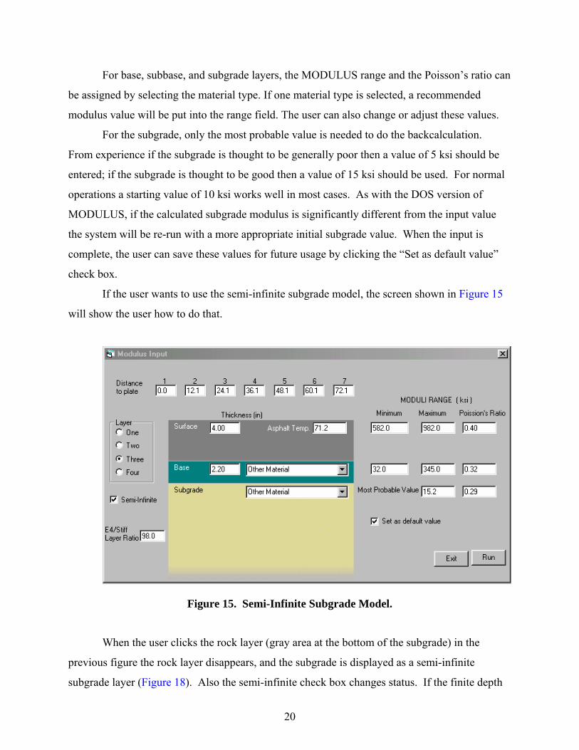
If the user wants to use the semi-infinite subgrade model, the screen shown in Figure 15
will show the user how to do that.
Figure 15. Semi-Infinite Subgrade Model.
When the user clicks the rock layer (gray area at the bottom of the subgrade) in the
previous figure the rock layer disappears, and the subgrade is displayed as a semi-infinite
subgrade layer (Figure 18). Also the semi-infinite check box changes status. If the finite depth
21
to bedrock model is used, the user can change the E4/stiff layer ratio to account for the stiff
relationship between the subgrade and the rock layer. In most cases, the modular ratio of 100 is
recommended as a reasonable value. However if the user suspects that the stiffening is caused
by a stiff clay layer then a subgrade/stiff layer modular ratio of 3 should be considered.
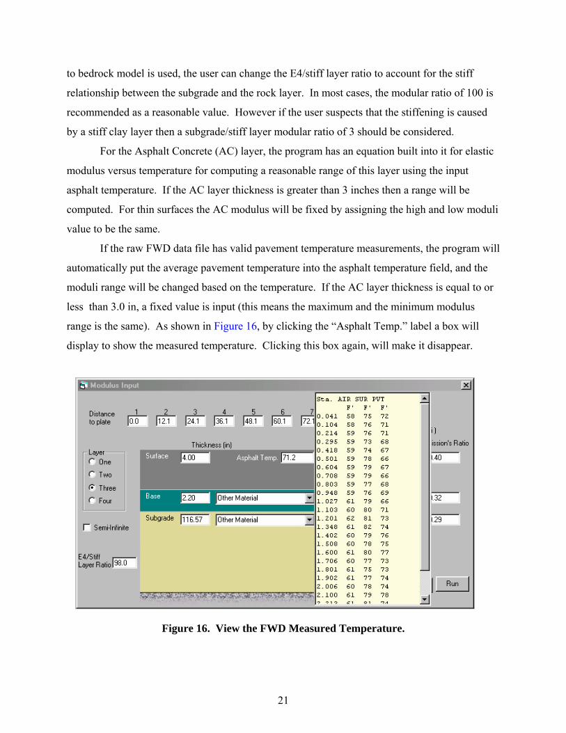
For the Asphalt Concrete (AC) layer, the program has an equation built into it for elastic
modulus versus temperature for computing a reasonable range of this layer using the input
asphalt temperature. If the AC layer thickness is greater than 3 inches then a range will be
computed. For thin surfaces the AC modulus will be fixed by assigning the high and low moduli
value to be the same.
If the raw FWD data file has valid pavement temperature measurements, the program will
automatically put the average pavement temperature into the asphalt temperature field, and the
moduli range will be changed based on the temperature. If the AC layer thickness is equal to or
less than 3.0 in, a fixed value is input (this means the maximum and the minimum modulus
range is the same). As shown in Figure 16, by clicking the “Asphalt Temp.” label a box will
display to show the measured temperature. Clicking this box again, will make it disappear.
Figure 16. View the FWD Measured Temperature.
22
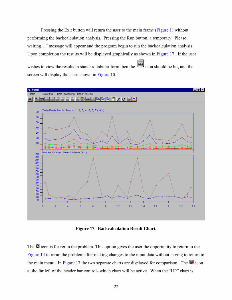
Pressing the Exit button will return the user to the main frame (Figure 1) without
performing the backcalculation analysis. Pressing the Run button, a temporary “Please
waiting…” message will appear and the program begin to run the backcalculation analysis.
Upon completion the results will be displayed graphically as shown in Figure 17. If the user
wishes to view the results in standard tabular form then the icon should be hit, and the
screen will display the chart shown in Figure 10.
Figure 17. Backcalculation Result Chart.
The icon is for rerun the problem. This option gives the user the opportunity to return to the
Figure 14 to rerun the problem after making changes to the input data without having to return to
the main menu. In Figure 17 the two separate charts are displayed for comparison. The icon
at the far left of the header bar controls which chart will be active. When the “UP” chart is
23
active the user can use the remaining icons to change what is graphed in the upper chart.
Initially the upper chart shows deflections at all seven sensors. To remove any of these from the
graph click any of the icons D1 thru D7 and that data will be removed from the plot. The
deflection data can be replaced by either load, error per sensor, or depth to bedrock by selecting
the other appropriate icons.
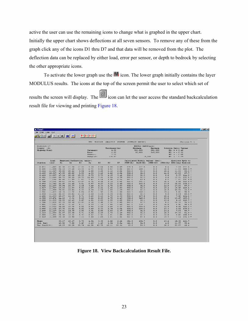
To activate the lower graph use the icon. The lower graph initially contains the layer
MODULUS results. The icons at the top of the screen permit the user to select which set of
results the screen will display. The icon can let the user access the standard backcalculation
result file for viewing and printing Figure 18.
Figure 18. View Backcalculation Result File.
24
Figure 18 shows the MODULUS outputs. The format is the same as the previous DOS
version MODULUS.
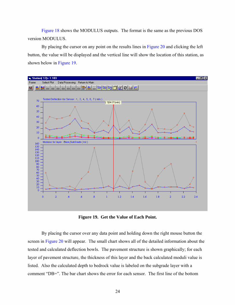
By placing the cursor on any point on the results lines in Figure 20 and clicking the left
button, the value will be displayed and the vertical line will show the location of this station, as
shown below in Figure 19.
Figure 19. Get the Value of Each Point.
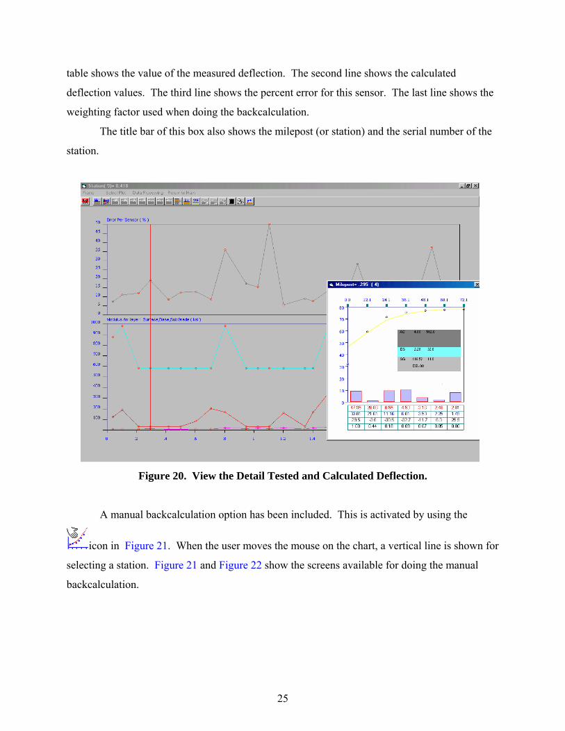
By placing the cursor over any data point and holding down the right mouse button the
screen in Figure 20 will appear. The small chart shows all of the detailed information about the
tested and calculated deflection bowls. The pavement structure is shown graphically; for each
layer of pavement structure, the thickness of this layer and the back calculated moduli value is
listed. Also the calculated depth to bedrock value is labeled on the subgrade layer with a
comment “DB=”. The bar chart shows the error for each sensor. The first line of the bottom
25
table shows the value of the measured deflection. The second line shows the calculated
deflection values. The third line shows the percent error for this sensor. The last line shows the
weighting factor used when doing the backcalculation.
The title bar of this box also shows the milepost (or station) and the serial number of the
station.
Figure 20. View the Detail Tested and Calculated Deflection.
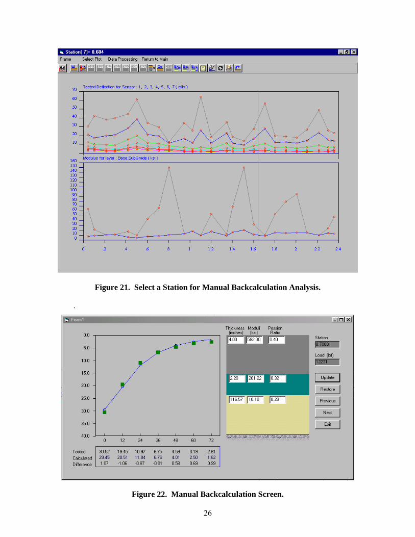
A manual backcalculation option has been included. This is activated by using the
icon in Figure 21. When the user moves the mouse on the chart, a vertical line is shown for
selecting a station. Figure 21 and Figure 22 show the screens available for doing the manual
backcalculation.
26
Figure 21. Select a Station for Manual Backcalculation Analysis.
.
Figure 22. Manual Backcalculation Screen.
27
The chart on the left of Figure shows the measured and calculated deflection bowls. The
right side shows the pavement structure. The bottom table shows the measured and the calculated
deflection values and the difference between these two values.
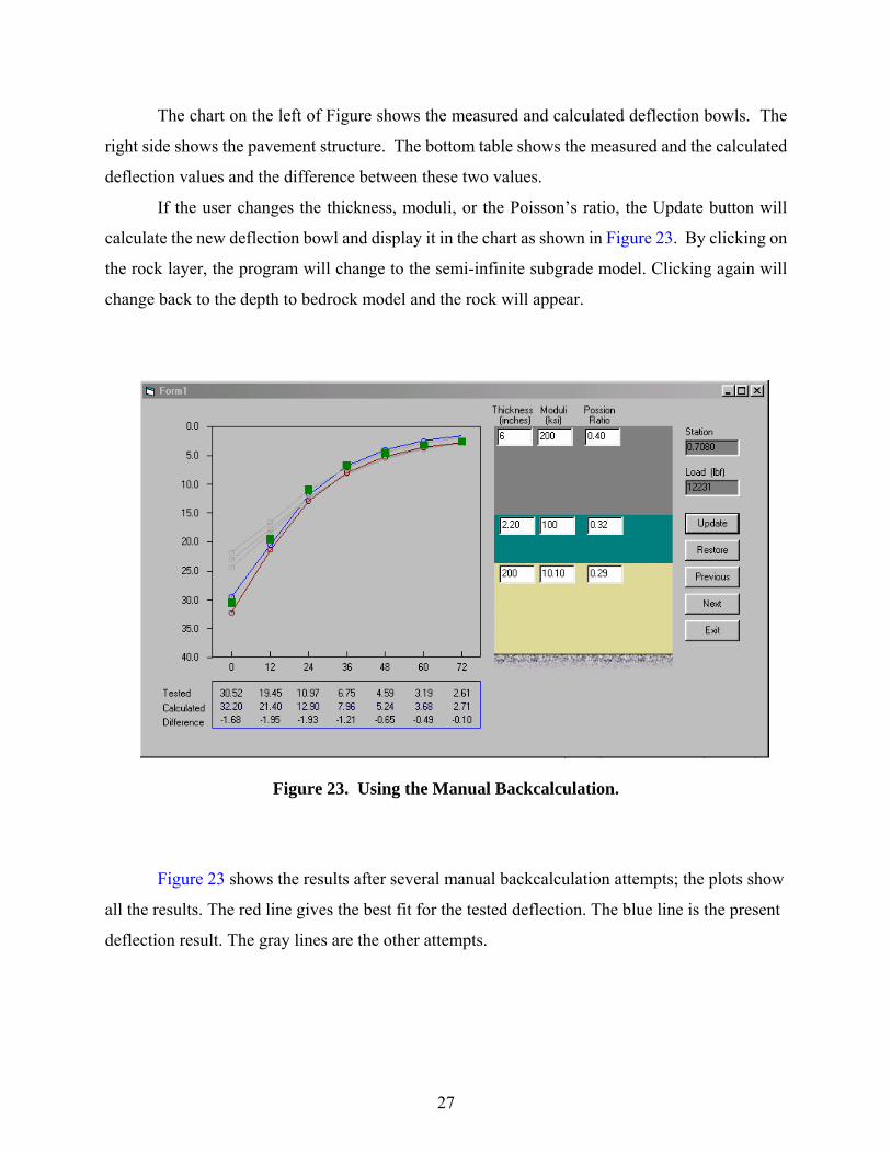
If the user changes the thickness, moduli, or the Poisson’s ratio, the Update button will
calculate the new deflection bowl and display it in the chart as shown in Figure 23. By clicking on
the rock layer, the program will change to the semi-infinite subgrade model. Clicking again will
change back to the depth to bedrock model and the rock will appear.
Figure 23. Using the Manual Backcalculation.
Figure 23 shows the results after several manual backcalculation attempts; the plots show
all the results. The red line gives the best fit for the tested deflection. The blue line is the present
deflection result. The gray lines are the other attempts.

29
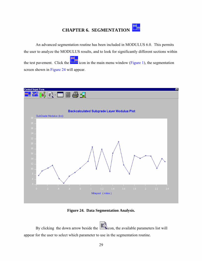
CHAPTER 6. SEGMENTATION
An advanced segmentation routine has been included in MODULUS 6.0. This permits
the user to analyze the MODULUS results, and to look for significantly different sections within
the test pavement. Click the icon in the main menu window (Figure 1), the segmentation
screen shown in Figure 24 will appear.
Figure 24. Data Segmentation Analysis.
By clicking the down arrow beside the icon, the available parameters list will
appear for the user to select which parameter to use in the segmentation routine.
30
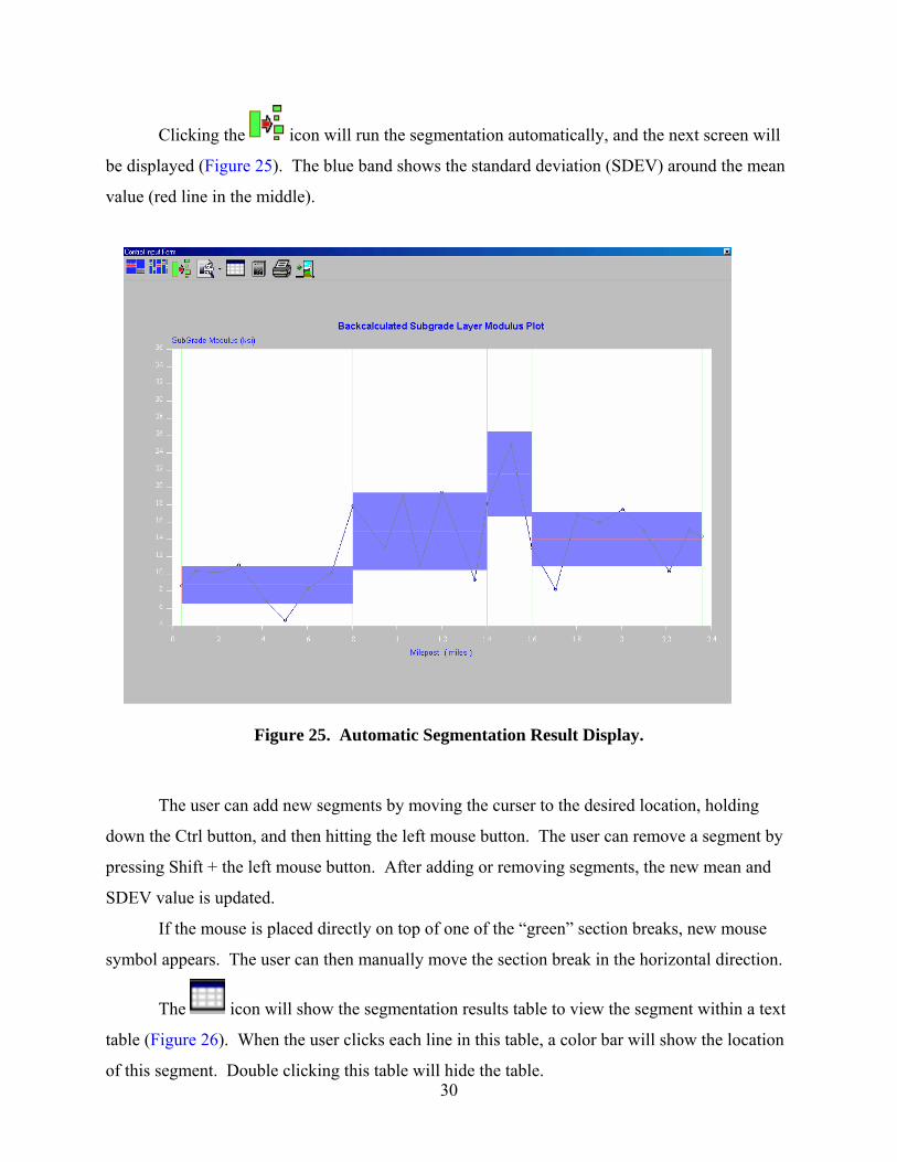
Clicking the icon will run the segmentation automatically, and the next screen will
be displayed (Figure 25). The blue band shows the standard deviation (SDEV) around the mean
value (red line in the middle).
Figure 25. Automatic Segmentation Result Display.
The user can add new segments by moving the curser to the desired location, holding
down the Ctrl button, and then hitting the left mouse button. The user can remove a segment by
pressing Shift + the left mouse button. After adding or removing segments, the new mean and
SDEV value is updated.
If the mouse is placed directly on top of one of the “green” section breaks, new mouse
symbol appears. The user can then manually move the section break in the horizontal direction.
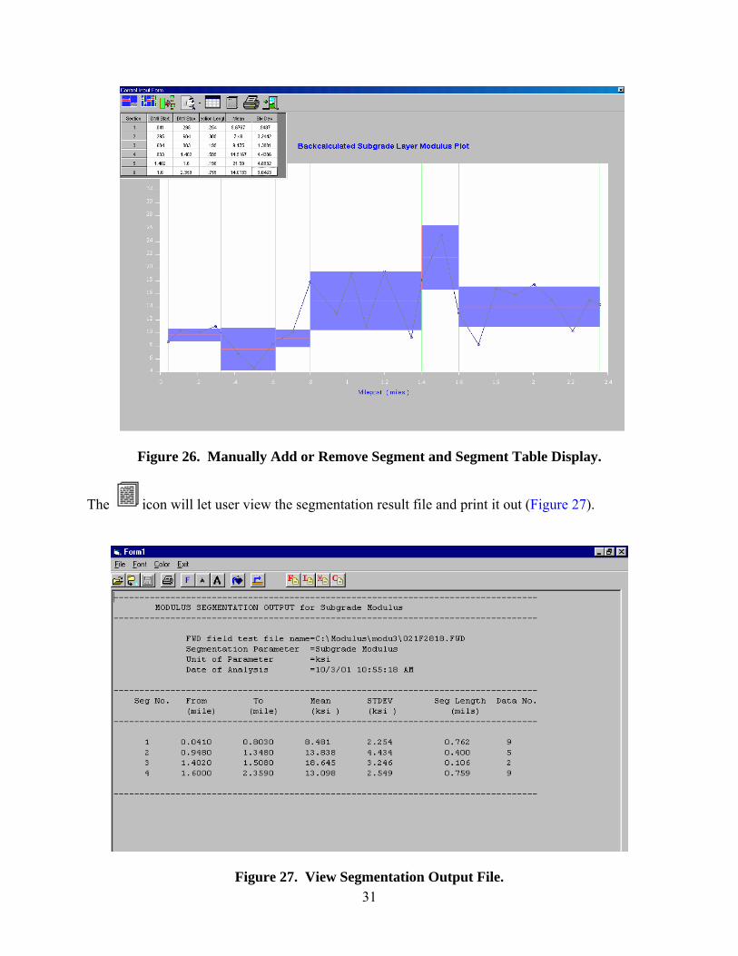
The icon will show the segmentation results table to view the segment within a text
table (Figure 26). When the user clicks each line in this table, a color bar will show the location
of this segment. Double clicking this table will hide the table.
31
Figure 26. Manually Add or Remove Segment and Segment Table Display.
The icon will let user view the segmentation result file and print it out (Figure 27).
Figure 27. View Segmentation Output File.

33
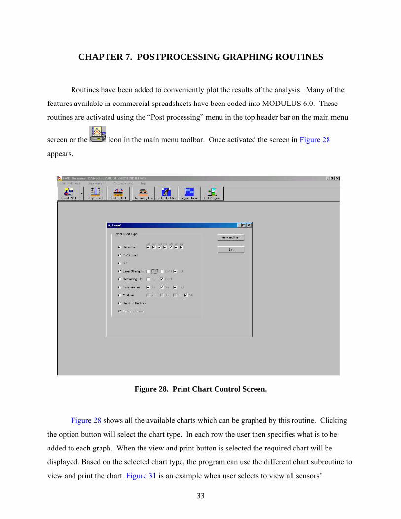
CHAPTER 7. POSTPROCESSING GRAPHING ROUTINES
Routines have been added to conveniently plot the results of the analysis. Many of the
features available in commercial spreadsheets have been coded into MODULUS 6.0. These
routines are activated using the “Post processing” menu in the top header bar on the main menu
screen or the icon in the main menu toolbar. Once activated the screen in Figure 28
appears.
Figure 28. Print Chart Control Screen.
Figure 28 shows all the available charts which can be graphed by this routine. Clicking
the option button will select the chart type. In each row the user then specifies what is to be
added to each graph. When the view and print button is selected the required chart will be
displayed. Based on the selected chart type, the program can use the different chart subroutine to
view and print the chart. Figure 31 is an example when user selects to view all sensors’
34
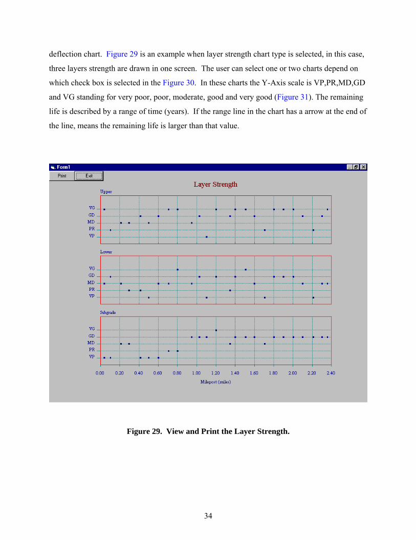
deflection chart. Figure 29 is an example when layer strength chart type is selected, in this case,
three layers strength are drawn in one screen. The user can select one or two charts depend on
which check box is selected in the Figure 30. In these charts the Y-Axis scale is VP,PR,MD,GD
and VG standing for very poor, poor, moderate, good and very good (Figure 31). The remaining
life is described by a range of time (years). If the range line in the chart has a arrow at the end of
the line, means the remaining life is larger than that value.
Figure 29. View and Print the Layer Strength.
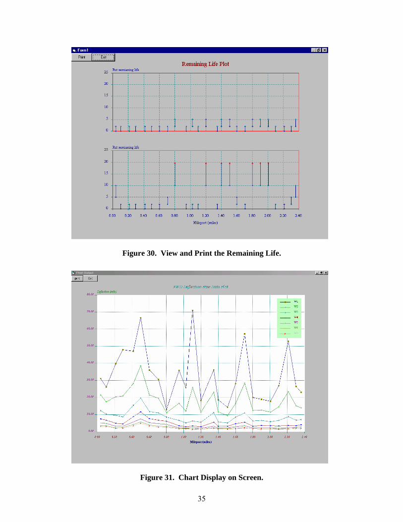
35
Figure 30. View and Print the Remaining Life.
Figure 31. Chart Display on Screen.
36
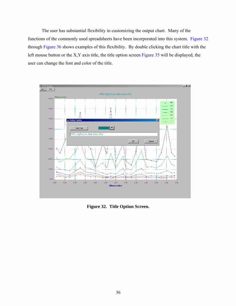
The user has substantial flexibility in customizing the output chart. Many of the
functions of the commonly used spreadsheets have been incorporated into this system. Figure 32
through Figure 36 shows examples of this flexibility. By double clicking the chart title with the
left mouse button or the X,Y axis title, the title option screen Figure 35 will be displayed, the
user can change the font and color of the title.
Figure 32. Title Option Screen.
37
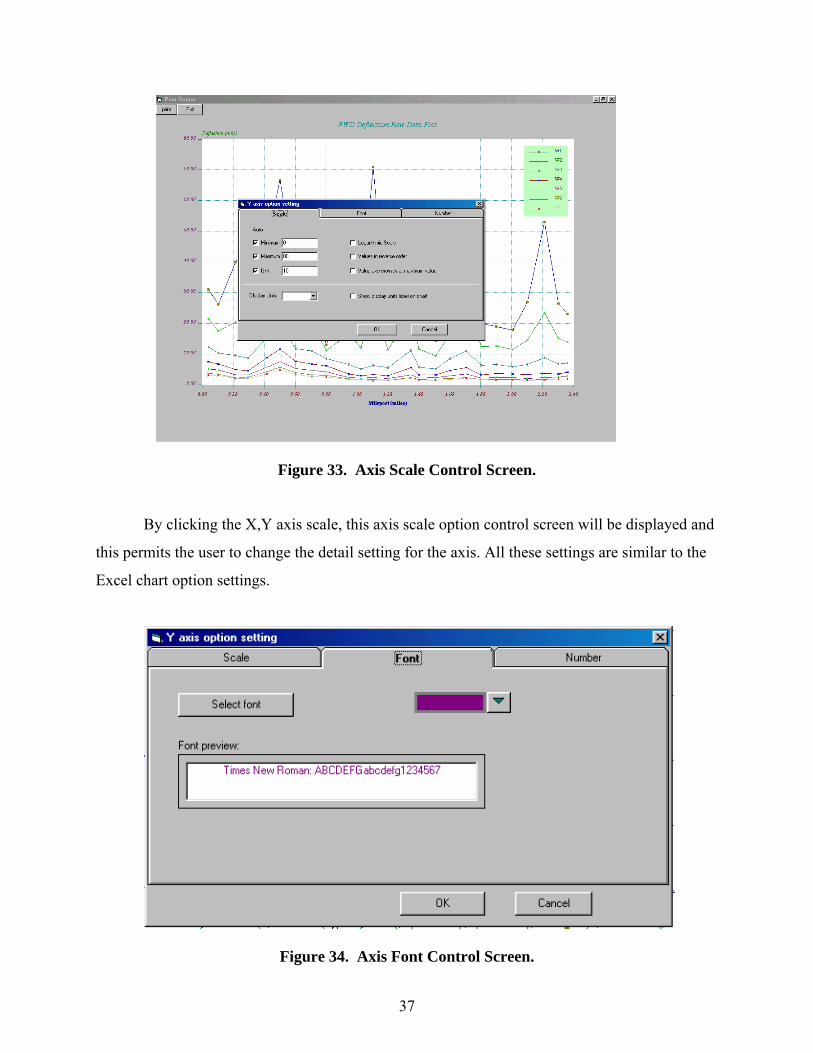
Figure 33. Axis Scale Control Screen.
By clicking the X,Y axis scale, this axis scale option control screen will be displayed and
this permits the user to change the detail setting for the axis. All these settings are similar to the
Excel chart option settings.
Figure 34. Axis Font Control Screen.
38
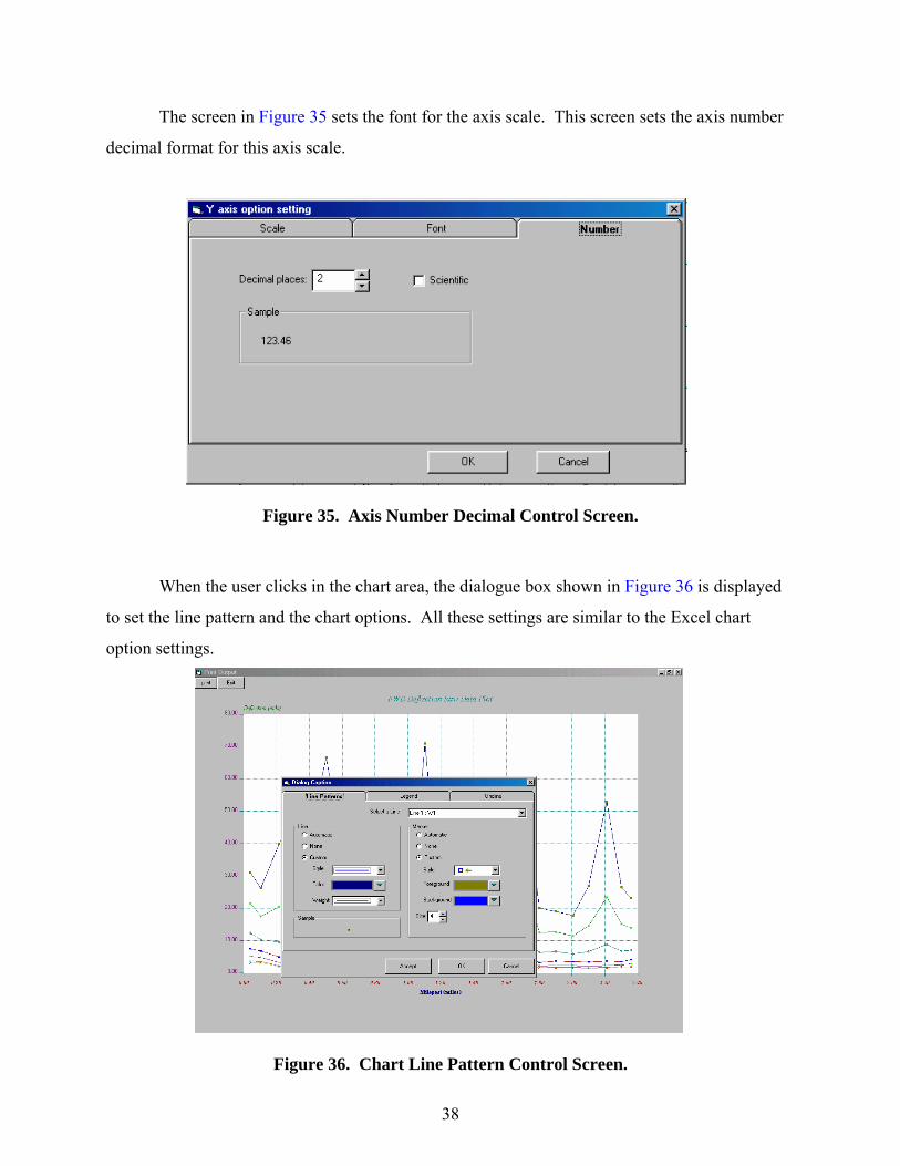
The screen in Figure 35 sets the font for the axis scale. This screen sets the axis number
decimal format for this axis scale.
Figure 35. Axis Number Decimal Control Screen.
When the user clicks in the chart area, the dialogue box shown in Figure 36 is displayed
to set the line pattern and the chart options. All these settings are similar to the Excel chart
option settings.
Figure 36. Chart Line Pattern Control Screen.
39
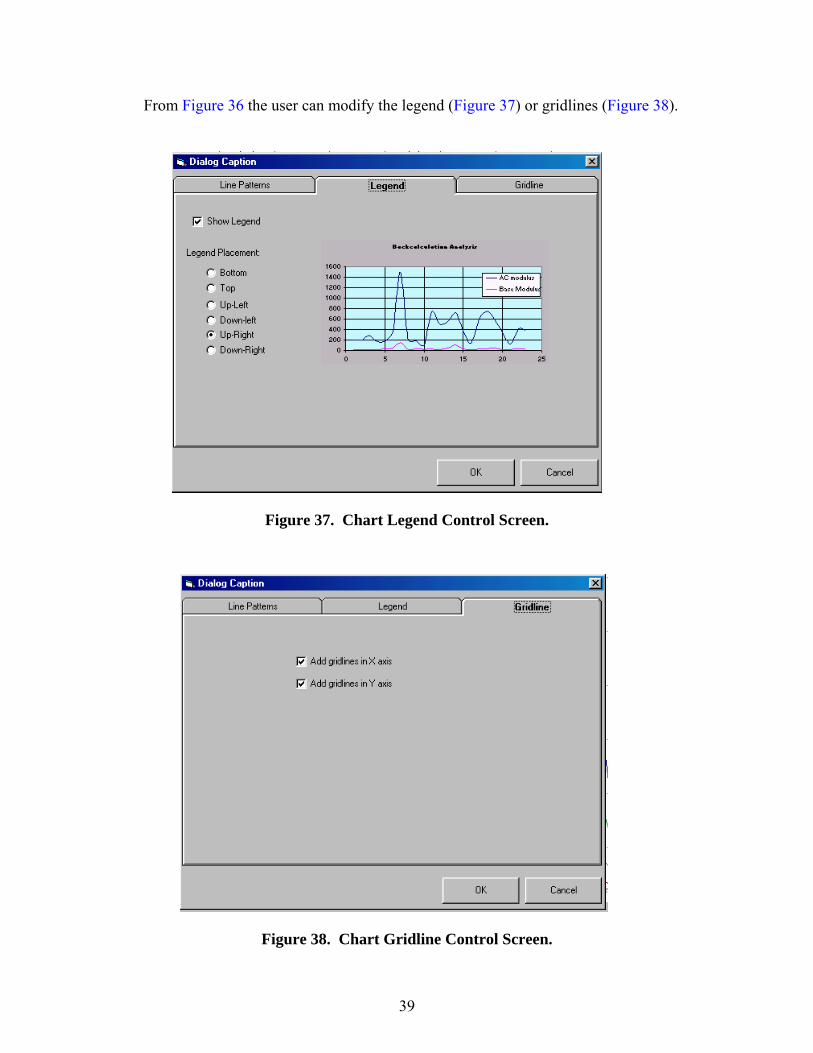
From Figure 36 the user can modify the legend (Figure 37) or gridlines (Figure 38).
Figure 37. Chart Legend Control Screen.
Figure 38. Chart Gridline Control Screen.


41
REFERENCES
1. C.H. Michalak and T. Scullion. MODULUS 5.0: User’s Manual, Research Report 1987-
1. Texas Transportation Institute, College Station, Texas, November 1995.