Embed Size (px)
Citation preview

AALTO UNIVERSITY
School of Engineering
Department of Energy Technology
Mohammad Mahmodul Hasan
Biomass based oxyfuel combustion in CHP power
plant with opportunity of oxygen storage system for
carbon capture and storage
Thesis submitted in partial fulfillment of the requirements of the degree of Master of
Science in Technology
Espoo, Finland
October 22, 2012
Supervisor: Prof. Mika Järvinen
Co-supervisor: Prof. Andrew Martin
Instructor: Dr. Timo Laukkanen and Dr. Loay Saeed
AALTO UNIVERSITY
SCHOOL OF ENGINEERING
PB 11000, 00076 AALTO
http://www.aalto.fi
ABSTRACT OF THE MASTER’S THESIS
Author: Mohammad Mahmodul Hasan 309332
Title of the work: Biomass based oxyfuel combustion in CHP power plant with
opportunity of oxygen storage system for carbon capture and storage
Department: Energy Technology
Professorship: Energy Technology Code: Ene-47
Supervisor: Prof. Mika Järvinen
Co-Supervisor: Prof. Andrew Martin
Instructor: Dr. Timo Laukkanen and Dr. Loay Saeed
Abstract:
Carbon dioxide (CO2) emission from coal-based power plants is one of the major
environmental concerns since coal will remain as a dominant source of energy for the
next few decades. Therefore, the CO2 emission requires to be decreased and move
towards renewable energy sources to meet the environmental and sustainability targets.
However, it will not be able to meet the worldwide energy demand because of the
limited commercialization of renewable energy sources. As coal is the most leading
energy source, it is necessary to divert a considerable phase of research work in CO2
capture and utilization for coal-based power plants to achieve the global environmental
targets.
In this thesis, overall features for power plant process modeling and optimization with
the provision of carbon capture, oxyfuel combustion and district heating have been
analyzed. The process model was designed and simulated by Prosim software changing
the key parameters of coal and biomass blending and various district heating loads. The
simulation results for the proposed power plant explain the effect of biomass co-firing
on net efficiency (heat and power) and power consumption for Air Separation Unit
(ASU), oxygen storage linked with grid electricity price and analysis of power to heat
ratio. From the analysis, increased net efficiency was originated with adding more
biomass with coal. This research work also focuses the general economic evaluation for
oxygen storage in relation to electricity and district heating price with optimization
software GAMS.
Most of the research works in this field are concentrating towards carbon capture and
storage only. The approach behind the thesis focuses to incorporate different variables
for a proposed system along with effect of selected key variables for the process
optimization.
Date: October 22, 2012 Language: English Number of pages: 73
Key words: Oxyfuel combustion, carbon capture, simulation, process optimization, oxygen storage

i | P a g e
Acknowledgements
First of all, I would like to thank the Almighty Allah for giving me the ability to
complete this thesis work and also for the opportunity to have M.S. degree.
I would like to express my appreciation to my supervisor Prof. Mika Järvinen for his
encouraging guidance and nice comments. I would thank Prof. Andrew Martin for his
nice suggestions. I do wish to express gratefulness to my instructors Dr. Timo
Laukkanen and Dr. Loay Saeed, who have guided me through the thesis work. Their
nice efforts have facilitated me to work with Prosim and GAMS software and broad
area of process simulation and optimization.
I gratefully acknowledge Reijo Kuivalainen, Foster Wheeler Energia Oy and CLEEN
Ltd’s CCSP programme for funding and supporting me.
I would like to thank Dr. Victoria Martin, Associate professor and Programme
Director, Erasmus Mundus SELECT for her academic cooperation and all staffs of
SELECT Programme in Finland and Sweden.
I must take the opportunity to thank all Researchers of the Research Unit: Energy
Engineering and Environmental Protection for their supports and good company in
the Coffee table. I want to thank my SELECT friends Sudip Kumar for sharing his
real experience from coal-based power plant and Nanda Kumar for clarification of
several features during thesis work.
Finally, my cordial gratitude is to my parents, my wife Kajal and my younger brother
Tarun for standing all the way in my side.
Espoo, October 22, 2012 Mohammad Mahmodul Hasan

ii | P a g e
Table of Contents
Acknowledgements ................................................................................................... i
Table of Contents ..................................................................................................... ii
List of abbreviations and notations ........................................................................ iv
List of Figures ......................................................................................................... vi
List of Tables ......................................................................................................... vii
1 Introduction ..................................................................................................... 1
1.1 Background ................................................................................................. 2
1.2 Research problem ........................................................................................ 4
1.3 Aim of the work .......................................................................................... 4
1.4 Scope of the work ........................................................................................ 5
1.5 Challenges ................................................................................................... 5
2 Carbon capture technologies and oxyfuel combustion ................................... 6
2.1 Types of capture technologies ...................................................................... 6
2.2 Oxyfuel combustion .................................................................................... 8
2.2.1 Characteristics of oxyfuel combustion .................................................. 9
2.3 Circulating Fludized Bed (CFB) boiler ...................................................... 12
2.4 Biomass blending with CCS ...................................................................... 14
2.5 District deating (DH) system in CHP plant ................................................ 14
2.6 Oxygen storage system .............................................................................. 17
2.7 Carbon capture and Storage ....................................................................... 17
2.7.1 Processing of CO2 .............................................................................. 17
2.7.2 Compression of CO2 ........................................................................... 17
2.7.3 Transportation of CO2 ........................................................................ 18
2.7.4 Storage of CO2 ................................................................................... 19
3 Methods .......................................................................................................... 21
3.1 System description .................................................................................... 21
3.1.1 Air Separation Unit (ASU) ................................................................. 22
3.1.2 Circulating Fluidized Bed (CFB) boiler .............................................. 23
3.1.3 Steam turbine ..................................................................................... 23
3.1.4 District heating system ....................................................................... 24

iii | P a g e
3.1.5 Carbon capture in the process model .................................................. 24
3.2 Simulation tool: Prosim process model ...................................................... 25
3.2.1 Blend of fuel in process model ........................................................... 25
3.2.2 Desiging parameters for DH load in process model............................. 26
3.2.3 Design cases for process model .......................................................... 27
3.3 Optimization tool: GAMS model ............................................................... 30
3.3.1 Formulation of model ......................................................................... 31
3.3.2 Objective function .............................................................................. 33
3.3.3 Equations for GAMS model ............................................................... 34
3.3.4 Operational methodology of oxygen storage ....................................... 36
4 Results ............................................................................................................ 37
4.1 Simulation results from process model ...................................................... 37
4.1.1 Relation between DH and net electricity ............................................. 37
4.1.2 Net efficiency versus biomass percentage with coal ............................ 41
4.1.3 O2 mass flow versus biomass percentage with coal ............................. 44
4.2 Optimization results from GAMS model ................................................... 45
4.2.1 Oxygen storage model ........................................................................ 45
4.2.2 Economic Evaluation considering O2 storage...................................... 47
5 Discussion ....................................................................................................... 49
6 Conclusion ...................................................................................................... 51
6.1 Future work ............................................................................................... 53
References .............................................................................................................. 55
APPENDICES ....................................................................................................... 59
APPENDIX A: Ongoing and proposed oxyfuel combustion projects ................... 59
APPENDIX B: Simulation results for all design cases ......................................... 60
APPENDIX C: Heat load duration curve ............................................................. 72
APPENDIX D: Elspot price for 2011 in Finland ................................................. 73

iv | P a g e
List of abbreviations and notations
ASU Air Separation Unit
CCS Carbon Capture and Storage
CFB Circulating Fluidized Bed
CHP Combined Heat and Power
CPU Carbon Compression and Purification Unit
CO Carbon monoxide
CO2 Carbon dioxide
DH District Heating
ETS Emission Trending Scheme
EU European Union
FG Flue gas
GAMS General Algebraic Modeling System
H2 Hydrogen
H2O Water
HP High pressure
HPC High pressure column
IGCC Integrated Gasification Combined Cycle
IP Intermediate pressure
IPCC The Intergovernmental Panel on Climate Change
kt Kiloton
kWh Kilowatt Hours
LHV Lower Heating Value
LP Low pressure
LPC Low pressure column
CNG Compressed natural gas
Mt Million tons
MW Megawatt
MWh Megawatt Hours
N2 Nitrogen

v | P a g e
NOX Nitrogen Oxide
O2 Oxygen
PF Pulverized Coal
RFG Recycled Flue Gas
SOX Oxides of Sulfur
USD United States Dollar
m mass flow
p pressure
P power
s second
T temperature
th thermal
e electrical
€ euro

vi | P a g e
List of Figures
Figure 1.1: World net electricity generation by fuel, 2008-2035 .................................. 2
Figure 1.2: World energy-related CO2 emission by fuel, 1990-2035 ............................ 3
Figure 1.3: Key technologies for reducing CO2 emissions ............................................ 3
Figure 2.1: Three categories of carbon capture technologies ...................................... 6
Figure 2.2: Progress of various oxyfuel pilot plants and demonstration projects ........ 8
Figure 2.3: Simple block of oxyfuel combustion ............................................................ 9
Figure 2.4: Diagram of a Circulating Fluidized Bed (CFB) boiler ............................ 13
Figure 2.5: CHP share of total national power production. ....................................... 15
Figure 2.6: Interface between CO2 capture and storage ............................................. 18
Figure 2.7: Trapping mechanism and timeframe for CO2 storage .............................. 20
Figure 3.1: Air separation unit (ASU) with 2 pressure columns ................................. 22
Figure 3.2: Process diagram for CO2 processing and purification ............................ 24
Figure 3.3: The proposed CHP power plant with CCS ............................................... 28
Figure 3.4: Overall system diagram including O2 storage with parameters and
variables ....................................................................................................................... 36
Figure 4.1: Relation between DH load and net electricity for design case 1 .............. 37
Figure 4.2: Relation between DH load and net electricity for design case 2 .............. 38
Figure 4.3: Relation between DH load and net electricity for design case 3 .............. 39
Figure 4.4: Relation between DH and net electricity for design case 4 ...................... 40
Figure 4.5: Change of net efficiency with biomass percentage (design case 1) .......... 41
Figure 4.6: Change of net efficiency with biomass percentage (design case 2) .......... 42
Figure 4.7: Change of net efficiency with biomass percentage (design case 3) .......... 42
Figure 4.8: Change of net efficiency with biomass percentage (design case 4) .......... 43
Figure 4.9: Change of O2 stream with biomass percentage (all design cases) ........... 44
Figure 4.10: Comparison between O2 storage and electricity price for year 2011 .... 46

vii | P a g e
List of Tables
Table 3.1: Blend of coal and biomass used in process model ..................................... 25
Table 3.2: Fuel analysis of coal and biomass.............................................................. 26
Table 3.3: DH load at plant side for process model .................................................... 27
Table 3.4: Design cases based on fuel mix and DH load ............................................ 27
Table 3.5: Assumption of parameters and data input .................................................. 29
Table 3.6: Key process parameters for Prosim model ................................................ 30
Table 3.7: Indices used in model ................................................................................. 31
Table 3.8: Sets required for the model......................................................................... 31
Table 3.9: Parameters used in GAMS Model .............................................................. 32
Table 3.10: Positive variables in GAMS Model .......................................................... 33
Table 4.1: Economic data used for process model ...................................................... 47
Table 4.2: O2 storage benefit potential for all design cases ........................................ 47

1 | P a g e
1 Introduction
Sustainable energy production is now an immense concern for the world. The reserve
of fossil fuels (oil, coal and natural gas) is depleting and renewable energy sources
(solar, wind, biomass, ocean wave and geothermal, etc.) are getting precedence for
power generation. However, fossil fuel will still be dominant (especially coal) over
the 21st century. In contrast, power generation from fossil fuel is one of the major
sources of greenhouse gases. Therefore, efficient usage of fossil fuel is a key question.
The carbon capture and storage technology includes the approaches by which
greenhouse gas like carbon dioxide (CO2) is captured from flue gas, mechanically
compressed and stored in the underground [1-2]. Oxyfuel combustion of coal is now a
promising technique, where coal burns with pure oxygen (O2) instead of air. In
addition, biomass can be used with coal to reduce fuel cost and positive effect on
environment [1,3].
Existing power plants are not equipped with the technologies of state of the art for
carbon capture. Authorities focus on flue gas cleaning and carbon tax. Carbon tax and
cost for scrubbing gas will increase in the future. On the other hand, oxyfuel
combustion and carbon capture method will reduce CO2 in the flue gas. This
combustion method has been conducted in several demonstration projects for power
generation plant since 2006 [1]. However, capture technology is still expensive.
Opportunities of the biomass based oxyfuel combustion and carbon capture highly
depend on precise results from the demonstration plants.
Energy production from conventional fossil fuel fired plants is the dominant
contributor to greenhouse gas emission. It is a well-known fact that greenhouse gas
emission can be reduced by the use of renewable energy sources. However, the
commercialization of the renewable energy sources is limited due to its intermittent
nature. Therefore, the role of the coal-fired power plants will remain dominant to
meet the global energy demand. As a result, the research associated with the emission
from the coal-fired power plants will be interesting field to pursue.

2 | P a g e
0.0
2.0
4.0
6.0
8.0
10.0
12.0
14.0
2008 2015 2020 2025 2030 2035
Liquids
Nuclear
Natural gas
Renewables
Coal
trill
ion
KW
h
Year
1.1 Background
In past and in foreseeable future, coal-based power plants will be the main sources of
electricity to satisfy the global energy demand, because 100 % transition to renewable
energy sources will be quite impossible within next few years. The current challenge
is to maintain the energy mix of coal-based power plants in a carbon-constrained
world by reducing the greenhouse gas emission from the utilization of coal as a source
of energy. To reduce CO2 emission from coal-based power plants, several
technologies or ideas are adopted like efficiency improvement of power plants,
oxyfuel combustion with flue gas recirculation, carbon capture and storage and co-
firing of coal with biomass [1,6,7,8,9]. This kind of research and development with
coal-based power plants is gaining interest among the big energy companies across
the globe. Therefore, the present thesis work will address this challenge of energy
industries to reduce CO2 emission from coal-based power plants.
In International Outlook Report 2011 [4], coal has been projected as dominant fuel for
electricity generation worldwide in future. Coal for electricity generation contributed
40% of total supply of electricity over the world in 2008. Unlike 2008, its share may
decline to 37% in the projected year of 2035. Figure 1.1 illustrates a clear domination
of coal in future energy sources for generating power.
Figure 1.1: World net electricity generation by fuel, 2008-2035 [4].

3 | P a g e
0.0
5.0
10.0
15.0
20.0
25.0
19
90
19
93
19
96
19
99
20
02
20
05
20
08
20
11
20
14
20
17
20
20
20
23
20
26
20
29
20
32
20
35
Bill
ion
me
tric
to
ns
Coal
Liquids
Natural gas
History Projections 2008
Year
Similarly, carbon dioxide (CO2) emission from coal will be large part in the projection
2035. Interestingly, coal share in worldwide CO2 emission indicates an inverse
pattern. Emission from coal accounts for 43% in 2008 and 45% in 2035 (projected).
Figure 1.2 shows that the most carbon intensive fossil fuel is still leading source of
CO2 emission, and no sign of changes will be observed until 2035 [4].
Due to the dominant characteristic of coal in electric power generation and CO2
emission in future, economic and environmental measures are greatly required to
control greenhouse gases with promising technologies. Carbon capture and
Figure 1.3: Key technologies for reducing CO2 emissions [5].
Figure 1.2: World energy-related CO2 emission by fuel, 1990-2035 [4].

4 | P a g e
storage (CCS) has vast potentiality to perform an important role in upcoming years.
Figure 1.3 represents International Energy Agency (IEA) Projection 2050 to reduce
CO2 emission. CCS will have 19% capability as key technology for combat to
declining CO2 level as well as global temperature [5].
1.2 Research problem
The objective for most of the researches done in this field was the investigation and
optimization of power plants with oxyfuel combustion and carbon capture only. In
this work, a slightly different formulation is used: “The objective is to design a multi
objective optimization routine of a co-firing (blend of coal and biomass) in combined
heat and power (CHP) plant considering oxyfuel combustion with 70% Flue gas
recirculation, traditional carbon capture with remaining 30 % flue gas, provision of
oxygen storage linked with grid electricity price and district heating provision as
variables”. This multi objective optimization results will provide a solid background
to make this new concept of carbon capture linked with distinctive variables
commercially feasible.
1.3 Aim of the work
The objective of the thesis focuses on development of optimization approaches using
multi objective variables, that will provide a scientific background for the
implementation of carbon capture and oxyfuel combustion concept in coal-based
power plants with environmental and commercial justification. The most critical part
of the optimization is the proper selection of the variables to make the results useful
for industries. It is also interesting from academic point of view to analyze and
optimize different types of variables related to carbon capture in fossil fuel power
plants.
5 | P a g e
1.4 Scope of the work
The focus of the thesis is to design a co-fired CHP plant with carbon capture to
address sustainability issues related with fossil fuel power plants. The methods
adapted to this work aim to solve the CO2 emission problems of coal-based power
plants along with commercial justification. The tasks in this research work are
formulated as follows:
(a) Selection of energy efficient Air Separation Unit (ASU)
(b) Investigation and validation for 70% recirculation of flue gas
(c) Optimization of oxyfuel combustion
(d) Incorporation of district heating system
(e) Provision for oxygen storage
(f) Linking the concept of oxygen storage with grid electricity price.
1.5 Challenges
In this thesis work, several distinctive variables are presented for the optimization
routine. The biggest challenge in this work is the appropriate incorporation of all these
different concepts or variables in simulation software Prosim 5.6 with accepted
justification model prepared by General Algebraic Modeling Software (GAMS) to
design a feasible solution. Moreover, there are several practical challenges for the
implementation of the optimization results, as listed below:
(a) Co-firing ratio of coal and biomass
(b) Burner design for oxyfuel combustion along with flue gas recirculation
(c) High energy consumption of ASU
(d) Dynamics of district heating price in the energy market
(e) Fluctuation of electricity price in the grid and oxygen storage concept.

6 | P a g e
2 Carbon capture technologies and oxyfuel combustion
2.1 Types of capture technologies
Carbon capture technologies can be divided into three categories: post-combustion,
pre-combustion and oxyfuel combustion [1,2,6,7,8]. These combustion methods have
different advantages and disadvantages. Figure 2.1 demonstrates these three types of
carbon capture methods in plant configuration.
Post-combustion technology refers to the approach of carbon scrubbing from flue
gas of the conventional pulverized coal-fired power plants by chemical absorption
with mono ethanol-amine (MEA) [1]. Regeneration of the chemical sorbent uses
about 80% of total energy of the system thus losing efficiency. However,
development and research are being conducted for better solvents and reduction of the
energy use in regeneration. Retrofitting to the existing plant is possible due to its
installation at downstream of the boiler and cleaning system of the flue gas [6].
Figure 2.1: Three categories of carbon capture technologies [1].

7 | P a g e
Secondly, in pre-combustion technique, capturing of carbon is executed before
combustion through gasification of coal. Coal is gasified to produce syngas containing
CO2, CO and H2. Furthermore, water-gas shift reaction generates CO2. H2 is
combusted in gas turbine. This combustion technique is combined with Integrated
Gasification Combined Cycle (IGCC), where heat recovery steam generator and
steam turbine are built-in [6]. Several experiments have been conducted for technical
and economic calculations that demonstrate better plant efficiency. In contrast, plant
construction requires high capital cost. There are few IGCC plants, but none of them
include carbon capture and storage (CCS) systems [1].
Finally, oxyfuel combustion technology is being considered as a promising
technique for carbon capture in conventional coal-based power plants [1,3,9,10]. This
combustion approach uses pure O2 rather than air. It results in a high portion of CO2
in flue gas and water vapor. When the water vapor is separated, CO2 becomes
available for elimination. Moreover, some fractions of flue gas recycles for reducing
the combustion temperature as pure O2 causes high temperature in the combustion
chamber [11].
This oxyfuel combustion method has several features those are significant for power
plants. It does not include chemical process. Furthermore, nitrogen-free flue gas
makes a difference. While separating O2 from air, nitrogen (N2) emits to atmosphere.
As a result, no N2 originated greenhouse gases (NOx) is found in the oxyfuel based
conventional power plants. Besides, separation of N2 has a direct effect on equipment
size and heat losses thus saving capital cost. Conventional power plants use air for
fuel combustion that leads high volume of N2 in flue gas. In power generation, N2
contained flue gas has no positive impact [1,11]. In addition, lower emission is
achieved in using oxyfuel combustion technique. Regular conventional boiler
technology can manage oxyfuel combustion methods. Retrofitting of oxyfuel
technology in existing power plants is being considered nowadays.

8 | P a g e
2.2 Oxyfuel combustion
Reduction of the CO2 got priority since 1990s especially in the power generation
industry. Abraham had proposed the concept of oxyfuel combustion in 1982, that was
considered for use in oil recovery [9]. Satisfied results from several pilot and
demonstration projects will contribute in commercialization of oxyfuel technology in
the coal-based power plant. Figure 2.2 displays different oxyfuel based projects over
the world that shows the increasing number of plants around the year of 2010.
Interestingly, no plant is still operated in full phase as commercial power generation
[12].
The pilot project all over the world ranges 0.3-3.0 MW (thermal) and proposed
demonstration projects varies from 30 MW (thermal) to 300 MW (electrical). More
plants can be seen in Appendix A.
Figure 2.3 demonstrates the fundamental concept of oxyfuel combustion, where coal
is burnt in O2-CO2 atmosphere (rather than O2-N2 atmosphere), then cleaned through
Figure 2.2: Progress of various oxyfuel pilot plants and demonstration projects [12].

9 | P a g e
gas cleaner and further sent for purification and compression. One portion of flue gas
returns to the burner for providing CO2 atmosphere with O2 [8-9].
Figure 2.3: Simple block of oxyfuel combustion (a-ASU, b- furnace & boiler, c & e- gas
cleaner, d- recycling flue gas, f- condenser, g- CO2 compression and purification) [9].
2.2.1 Characteristics of oxyfuel combustion
Oxyfuel combustion is one of three separation methods that results in the reduction of
greenhouse gases. Oxyfuel combustion method mostly emphasizes on the fossil fuel
based power plants. However, this separation method triggers the decreasing
efficiency of a power plant. The efficiency loss ranges 9-13%. However, it is likely to
convert 7-11% by optimization of the plant. The nature of oxyfuel combustion differs
from conventional air combustion in several ways. The furnace gas environment is a
mixture of O2 and CO2 for oxyfuel combustion. Unlikely, air combustion takes place
in O2-N2 environment. The characteristics include [9]:
2.2.1.1 Recycled flue gas (RFG) ratio
The main parameter for firing condition is flue gas ratio where a certain percentage of
CO2 adds to O2 in burner and leads to change in temperature and heat transfer.
Similarly, CO2-H2O retains higher specific heat capacity and different radiation and

10 | P a g e
absorption characteristics. As a result, it is very important to select a range of flue gas
ratio that will compensate the temperature characteristic of air combustion.
Remarkably, many pilot and demonstration projects all over the world have been
using the RFG ratio in the range of 0.6 - 0.85 [9,11].
2.2.1.2 Temperature of RFG
The temperature of flue gas has an impact on the combustion in relation to change the
temperature of oxidant flow as pure oxygen (approximately 95%) mixes with RFG.
Furthermore, the flue gas (CO2-H2O stream) mixed with oxygen affects the heat flux
through boiler and boiler efficiency [11]. It has been studied that the temperature of
the flue gas ranges over 100 °C to 400 °C considering different types of coal. For
instance, the flue gas temperature for South African coal burnt ranges from 100 °C
(RFG ratio 65.8%) to 400 °C (RFG ratio 68.6%). In contrast, flue gas shows 100 °C
(RFG ratio 67.8%) and 400 °C (RFG ratio 71.7%) for Lusatian lignite. However, RFG
temperature from the technically realistic purpose can be 200 °C – 400 °C. In that
situation, the RFG ratio should be around 68-70% [9].
2.2.1.3 Oxygen concentration
While mixing with RFG in burner, high percentage of O2 is required for better heat
balance [9]. It should be considered that impact from CO2 on coal ignition takes place
if RFG ratio and burner aerodynamic are not properly optimized. Several studies
show that high percentage of CO2 environment causes retardation in coal ignition
[13]. Moreover, less non-condensable impurities are found in CO2 stream to capture
while high percentage (more than 90%) of oxygen passes to the boiler. The optimal
level of O2 purity is 95%, which has been reported in several research works.
However, argon with some traces of N2 is also observed in oxygen production from
ASU [11]. Better improvement in burnout has the possibility to happen in high
concentration of O2. But, sufficient O2 is required to pass into the burner to ensure
adequate ignition and flame stability [7].

11 | P a g e
2.2.1.4 Heat transfer
The characteristic of heat transfer in oxyfuel combustion is not similar as a
conventional power plant. However, heat transfer is also related to the RFG ratio. A
bit higher RFG ratio provides better heat transfer in the oxyfuel combustion [9]. To
achieve better heat transfer, a reasonable RFG ratio should be adopted. In case of heat
transfer, radiation is an important factor. CO2, H2O and different particulate matters
(for instance, char, soot and fly ash particles) activate radiative heat transfer.
Moreover, high concentration of CO2 and H2O mixture in boiler causes different
emissive nature resulting manipulation of radiative heat transfer and absorption of
heat in coal combustion [8,14]. The complex feature of heat transfer also considers
the percentage of CO2 and H2O. As CO2-H2O mixture has high specific heat capacity
than N2, the mixture enables to retain more heat and contributes high heat transfer in
convection section. However, lower amount of gas compared to air combustion and
high heat transfer in radiative section results in decreased temperature in furnace exit
gas. These features also act in decreasing heat transfer in convective section of boiler.
Optimization is required in heat transfer in convective and radiative section of boiler
to achieve efficient operation [1,9].
2.2.1.5 Combustion characteristics
From the findings of several research works, delayed ignition has been observed
comparing to firing in air. However, situation changes when temperature increases.
Interestingly, high percentage of O2 indicates a higher rate of burnout of coal and
biomass blends. Burnout of this blend in 79% CO2-21% O2 is less than burnout in
70% CO2-30% O2. Higher O2 concentration has a vital effect in char combustion rate
and ignition temperature [7-8]. Lower ignition temperature caused by high O2 rate
provides higher combustion time that turns in reaching higher burnout values. In
addition, burnout value increases with more blending of biomass with coal. However,
ignition temperature increases in O2-CO2 atmosphere compared to O2-N2 (air)
atmosphere due to higher specific molar heat of CO2 in comparison to N2 [3,7]. It
should be considered that biomass has lower calorific value and moisture content is

12 | P a g e
higher than coal in firing. Due to these properties, declining rate of flame temperature
may happen and radiative heat flux can be affected and thus reducing the oxidation
rate. Furthermore, significant impact of ignition temperature should get priority in the
high blending of biomass concentration [3].
2.2.1.6 Pollutant formation
NOx Formation:
Formation of NOx during combustion is a complex phenomenon. The factors causing
the formation of NOx includes, flame condition, O2 concentration and flame
temperature. Nitric oxide (NO) covers 95% of total NOx. Decreased value of NOx was
found in several pilot-scale projects during oxyfuel combustion. The phenomenon
happens due to the absence of N2 gas in combustion atmosphere and decomposition of
NOx through the RFG (NOx is contacted with hydrocarbon generated in reducing
atmosphere) [15]. Besides, combustion mode and combustion temperature also result
in reduction of NOx. Technology used in the conventional coal power plants can be
utilized in oxyfuel based coal power plant [8-9].
2.3 Circulating Fluidized Bed (CFB) boiler
CFB boiler is considered as a matured technology in the conventional power plants.
The advantages of CFB boiler include better environmental performance and
flexibility to use different types of fuels. The characteristics including better mixing
of fuel, low air excess and good air staging enable CFB boiler for considering
combustion purpose and reduction for NOx emission. Furthermore, limestone used for
Sulphur capture also performs well due to good mixing. Bed materials inside the CFB
boiler demonstrate 90-98% of blending of fuel and bed materials. Sand and dolomite
are used as common bed materials. Better combustion takes place with low air excess
(lambda ranges over 1.1-1.2 for CFB plants) due to mixing and concentrated heat
transfer. However, combustion temperature should be kept in the ranges of 650 °C-
900 °C for preventing ash sintering in bed. CFB boiler is one of the best options for

13 | P a g e
using the wide range of fuel as good mixing is achieved through the bed. Particle size
of fuel should be less than 40 mm [16].
In addition, biomass blending with coal burns well in CFB. As a result, CFB boiler is
one of the best choices for combustion coal and biomass together for the characteristic
of fuel flexibility, longevity of combustion time and smooth combustion temperature
[17]. However, more research works are required in some areas that have been
proposed in many reviews includes [9]:
1. Combustion behaviors
2. Emission formation
3. Fouling, slagging and corrosion
4. heat transfer analysis
5. Validation of modeling and design tools.
Figure 2.4 presents diagram of a CFB boiler along with superheater, Economizer and
air-preheater [18].
Figure 2.4: Diagram of a Circulating Fluidized Bed (CFB) boiler [18].

14 | P a g e
2.4 Biomass blending with CCS
As a source of renewable energy, biomass is used for balancing CO2 emission. Using
biomass as single fuel or blending with other fuels contributes in reducing CO2 gases.
While burning the biomass, combustion generated CO2 gas is recycled to the
atmosphere due to containing carbon in biomass in its life cycle. This energy source is
accepted as carbon neutral. Co-firing of biomass with coal is getting priority in CHP
plant incorporated with environmental friendly combustion and emission behaviour.
Minor modification is required for co-firing coal with biomass. Moreover, using
biomass in blending for combustion provides the scope to utilize biomass residue
instead of land filling [3,17]. Maximum 10% of biomass blending is recommended
due to particle sized constraints [19]. Biomass portion approximately 5% in co-firing
does not cause any remarkable problem. On the other hand, high biomass percentage
in co-firing (approximately 30%) may create problems in combustor like slagging and
fouling [20].
In case of CCS strategies, the carbon neutral biomass can be easily adopted with co-
firing. Combination of biomass with coal will contribute in removal of CO2 emission.
In addition, higher efficiency and lower cost are achievable in co-firing [19]. As there
are no 100% efficient technologies available for CO2 capture from flue gas, biomass
usage in co-firing can compensate the losses and enable oxyfuel based CCS as net
zero carbon emission [2].
2.5 District heating (DH) system in CHP plant
The combined heat and power concept mainly considers the simultaneous usage of
heat and power from a source of fuel. Both types of demand for electricity and heat
for residential area, city and industrial level are met up from a single CHP plant,
where CHP is focused as a source of heat as a by-product with generation of
electricity [21]. The CHP technology is considered as a favorable system where large
portion of supplied fuel (70-95%) is used for both electricity and heat generation. In

15 | P a g e
this system, the share of electricity generation is 20-50% considering the fuel and
available technologies. In contrast, only 35-55% of fuel is driven for generation of
electricity and rest of the fuel ends as useless product [16]. More than 100 million
people over the EU and CEE countries get DH facilities. Moreover, DH system is
considered as a significant product for CHP plant, especially in Western Europe. For
instance, 75% DH supply is generated from CHP plant in Finland. Figure 2.5
demonstrates the several countries, like Denmark, Finland, Russia, Latvia and the
Netherlands have got success in CHP features, where the expansion of CHP usage
was achieved for 30-50% of total power generation [21].
Figure 2.5: CHP share of total national power production. (Data merged from years
2001, 2005, 2006) [21].
However, the highly integrated system of CHP and DH operates at low cost so that
earning of a huge amount of money is possible [22]. A number of advantages DH
systems offer including [21-23]:
Flexibility of fuel use: In DH system, one of the prominent advantages is a
wide range of fuel usage. Co-firing (blending of different fuels) of cheap fuel
contributes in economic advantage in DH system.
CH
P S
har
e (
%)
16 | P a g e
Usage of waste heat: Opportunities related to using waste heat for generating
hot water for residential heating has enabled DH system to incorporate with
CHP plant.
Co-generation for economic benefits: Establishment of power plant and
district heating together bring the economic benefits into light. Unit
investment, operational and maintenance cost gradually declines compared to
single unit. Furthermore, thermal efficiency is usually high in CHP plant.
Better environment in urban area: While generating electricity and usable
heat from the single CHP plant, various environmental parameters of air,
water and soil quality will be better. Less pollution from a CHP plant is one of
the promising characteristics from environmental view [24].
Higher efficiency: The CHP plant for co-generation has higher net efficiency
than a conventional power plant. The net efficiency for CHP plant ranges
80%-90%, whereas the normal power production unit has comparably lower
efficiency like 30%-50%.
As, limit imposes for electricity generation due to heat demand in DH system, CHP
plant gives the opportunities to earn a high profit in electricity generation keeping
high electricity to heat ratio when electricity price is high [24]. In contrary, the DH
suppliers are facing some business issues like reducing their business to some extent.
Reducing heat demand for implementation of different energy conservation measures,
increased number of low-energy houses and finally comparably hot and warm
climate. However, this problem can be eliminated with a CHP plant where a trade-off
is balanced between DH system and electricity production. Converting process
technologies between electricity and DH system leads a reduction trend of resource
utilization and greenhouse gases emission [25].

17 | P a g e
2.6 Oxygen storage system
Oxygen storage system in oxyfuel combustion method is a relatively new concept. In
oxyfuel combustion, pure O2 is required that ASU produces. Due to high electricity
consumption by this unit along with power plant, the concept of the O2 storage system
is considered. Liquid O2 storage may be better solution where oxyfuel based power
plant can use stored O2 considering demand and production of electricity in relation to
boiler load. It is also possible to switch from the oxyfuel-based combustion to air
firing mode within short time if ASU fails to operate. Moreover, O2 storage system
with electricity price is also now as new research area to explore. Power plant and
ASU for continue O2 production along with the storage system can be significant
option in future [1].
2.7 Carbon capture and storage
2.7.1 Processing of CO2
The CO2 stream will be transported through the pipeline. Before passing to pipeline
and reservoir, it should be specified with pressure and temperature. High pressure is
recommended for overcoming the frictional and static pressure drops. Furthermore, it
is essential to conduct precaution of risk of flashing of gas in the whole process. For
conditioning the CO2 flow, the suggested ranges of pressure include 80-120 bar and
temperatures 0-50 °C. The temperature should be above the critical temperature of
CO2 ( 31.1 °C) [1].
2.7.2 Compression of CO2
Acquiring CO2 from flue gas and compression requires intensive energy like
operation of oxygen production in ASU. Usually, electrical efficiency declines
approximately 2-3% point. The factors like compressor efficiency, a significant
amount of impurities in CO2 lead the changing of power consumption in CPU.

18 | P a g e
Figure 2.6 shows the interface between CO2 capture and storage [26].
2.7.3 Transportation of CO2
Transportation of CO2 is possible through pipelines and ship in form of gas as well as
through pipelines, tanker and ships as a liquid form. From economic perspective,
pipelines as a medium of CO2 transport are cost effective. Similarly, 1-5 Mt of CO2
can be transported in a year over 100-500 km [2].
2.7.3.1 CO2 transportation by pipeline
Transportation of supercritical CO2 through pipeline is proved technology. 50 Mt of
CO2 is transported per year by long-distance pipeline of 5600 km (diameters up to
0.762 meters) all over the world.
Dehydration is executed before passing into pipelines in relation to reduce corrosion
risk and dry CO2 cannot be activated for corrosion due to steel made pipelines. The
largest Cortez pipeline in United States can handle 30 Mt of CO2 over 800 km per
year. On the other hand, projection for Europe is considering that 30000 km-150000
km of pipeline is required for transporting CO2. In several technical papers, the
Figure 2.6: Interface between CO2 capture and storage [26].

19 | P a g e
estimations for CO2 transportation range from USD 2/t CO2 to USD 6/t CO2 (100
km/year) for 2 Mt. However, prices differ from USD 1/t CO2 to USD 3/t CO2 (100
km/year) for 10 Mt [2].
2.7.3.2 CO2 transportation by Ship
CO2 can be transported by ship with a capacity of 10 kt to 50 kt and flexibility of
collection and gathering product from different sizes of sources. It turns the reduction
for the infrastructure capital cost. While transportation by ship, compressed natural
gas (CNG) carriers or semi-refrigerated tank is used. The cost for transportation in
ship ranges from USD 15 (for 1000 km) to USD 30 (5000 km) per ton of CO2 [2].
2.7.4 Storage of CO2
IPCC demonstrate three mechanisms for CO2 storage in their report. Those trapping
mechanisms are as follows [2]:
1. Physical trapping: Physical trapping refers to the immobilization of gaseous
or supercritical phase of CO2 that can be trapped in the geological formation
of two types; namely, static trap that takes place in the structural trap and
porous structure keeps residual gas.
2. Hydrodynamic trapping: CO2 with very low motions may migrate upward
and can be kept in intermediate layer. This mechanism is better for vast
quantities of CO2. This mechanism limits the risk of leakage from the
formation [1].
3. Chemical trapping: In this type of storage mechanism, CO2 is trapped by the
ionic trapping or dissolution with water or hydrocarbon. Besides, chemical
reaction happens with mineral that refers mineral trapping. Similarly, CO2 is
adsorbed on the mineral surface as called adsorption trapping.

20 | P a g e
Figure 2.7 represents the different types of trapping mechanisms those have been
mentioned before. The physical trapping is considered as the key mechanism under
the injection period retains several decades. However, with no risk of leakage
phenomenon, CO2 storage lasts for hundreds or thousands of years [2].
Figure 2.7: Trapping mechanism and timeframe for CO2 storage [2].

21 | P a g e
3 Methods
3.1 System description
The technologies that are developed for CO2 capture and sequestration from coal-fired
plants including: CO2 capture from conventional plants by scrubbing the flue gas,
oxyfuel combustion and IGCC with an air separation unit to provide O2 [6]. However,
in the present analysis the proposed power plant considers the following concepts:
Co-firing with coal and biomass
Oxyfuel combustion with recirculation of flue gas
CO2 capture by conventional compression process
Storage of oxygen for linking of grid electricity price.
Finally, connecting all these concepts together in one power plant will be very
interesting from optimization points of view considering both sustainability and
economic factors.
The proposed system is a conventional power plant developed in simulation software
Prosim 5.6 where standard tools with CFB boiler, steam turbines and necessary
arrangements for oxyfuel combustion, flue gas recirculation and CO2 capture have
been included [27].
The main components of the proposed power plant are:
Air Separation Unit (ASU)
CFB boiler with air-preheater and economizer
Steam turbines with high pressure (HP), intermediate pressure (IP) and two
low pressure (LP) modules
District heating source by taking tapping after first LP turbine
Compression and purification unit (CPU).

22 | P a g e
The characteristic of the each subsystem is described below:
3.1.1 Air Separation Unit (ASU)
The Air separation unit (ASU) will separate atmospheric air into its primary
components, typically O2 and N2. Among various technologies in the separation
process, cryogenic distillation technology is used in this proposed plant. The
separated oxygen from this unit will be directly provided to the boiler burner that acts
as a secondary air for the combustion.
The cryogenic separation process requires an integration of low-pressure column
(LPC) and high-pressure column (HPC). The air is first compressed, and then the
pressurized air is liquefied to separate O2 and N2 in turn in the columns according to
their boiling temperatures. This ASU is a very energy intensive unit and electricity
consumption proportionally increases with the purity of O2 [28-29].
Figure 3.1: Air separation unit (ASU) with two pressure columns [29].

23 | P a g e
3.1.2 Circulating Fluidized Bed (CFB) boiler
The fluidized bed boiler consists of a sand bed where fuel is introduced and
combusted. The combustion air blows through the sand bed from an opening at the
bottom of the bed. The main advantage of these types of boilers is the fuel flexibility.
Biomass can also be co-fired with low-grade coal. In this case, the special designed
burners are used with a provision to incorporate 70 % recirculation of flue gas along
with fuel (coal and biomass) and combustion air.
The simulation model of CFB boiler consists of five parts: burner, superheater (2
nos.), economizer, air preheater and evaporator. In the burner module, the parameters
that are incorporated are fuel (coal and biomass), secondary air (pure O2 from ASU)
and 70 % recirculated flue gas. In an actual power plant, the mixture of recirculated
flue gas in the burner needs a lot of auxiliary systems and connections. The separated
O2 is preheated in air preheater to have temperature close to the recirculated flue gas.
Moreover, in conventional power plants, the temperature of the air (oxygen) is
increased by recovering heat from flue gas to enhance boiler efficiency. Two sets of
superheater namely, primary and final superheater are used to produce superheated
steam that will drive the steam turbine. The feed water generated from the
condensation of steam is preheated in economizer with the exit flue gas to improve
boiler efficiency. In the evaporator, the steam water mixture is formed by recovering
heat from combustion and finally, the steam is separated in the boiler drum and sent
directly to superheater for further superheating.
3.1.3 Steam turbine
There are four modules of steam turbine namely; HP, IP and two LP turbines
incorporated in the system to generate electrical power. Two extractions are taken for
feed heating system – one from IP turbine exit, and the other one is from an
intermediate stage in the first LP turbine. A considerable part of steam (around 75% at
24 | P a g e
full load condition) from the exit of first LP turbine is used to supply heat for district
heating system.
3.1.4 District heating system
The concept of combined heat and power plant adopts to increase the overall
efficiency of the co-generation power plant. In a conventional condensing power
Plant, a huge quantity of heat is wasted in the condenser. Therefore, the proposed
concept will utilize the heat to fulfill the district heating need and enhances the overall
efficiency of the plant.
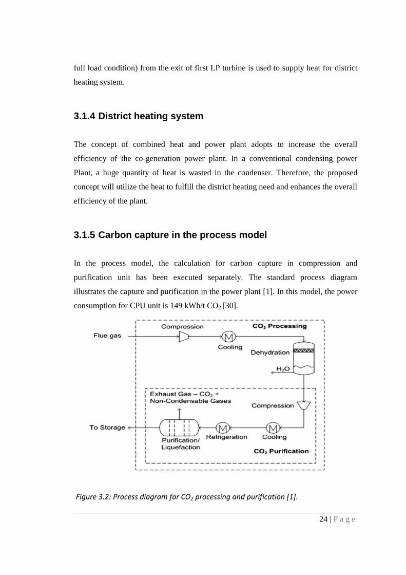
3.1.5 Carbon capture in the process model
In the process model, the calculation for carbon capture in compression and
purification unit has been executed separately. The standard process diagram
illustrates the capture and purification in the power plant [1]. In this model, the power
consumption for CPU unit is 149 kWh/t CO2 [30].
Figure 3.2: Process diagram for CO2 processing and purification [1].

25 | P a g e
3.2 Simulation tool: Prosim process model
After constructing the process model with simulation software Prosim 5.6, various
parameters and data have been selected and assumptions have been considered based
on literature review, objectives and goal of this proposed power plant. These data
were inserted into the Prosim model for simulation. The following works have been
performed for simulation activities.
1. Preparing the Process model with Prosim
2. Selection and verification of data to be used
3. Parameters identification
4. Assumption taken with consideration of literature review
5. Four design cases selection within the same process model
6. Conversion of design model to off-design mode
7. Changing parameters (DH load and fuel blend) in every design case
8. Simulation run and cross checking the data for validation.
3.2.1 Blend of fuel in process model
In this process model, fuel blending for co-firing has been categorized into four types.
Every type is denoted as ‘Fuel mix’. Every fuel mix has the different percentage of
coal and biomass. However, the total percentage will always be 100%. Table 3.1
represents the four types fuel mix considering coal and biomass value.
Table 3.1: Blend of coal and biomass used in process model.
Blend of fuel Coal Biomass
Fuel mix 1 100% 0%
Fuel mix 2 95% 5%
Fuel mix 3 90% 10%
Fuel mix 4 85% 15%

26 | P a g e
Table 3.2 shows the fuel analysis of coal and biomass used in this process model.
Analysis has been given in dry basis. Default value of the simulation programme has
been used. From Table 3.2, it is noticeable the biomass contains a high percentage of
O2 (42.5% dry wt.) whereas coal has low content of O2 (9.1% dry wt.). Due to high
content of O2, biomass has low energy density, and higher moisture also lowers the
energy content [19]. Furthermore, high moisture content in biomass accounts for
moderate level of carbon.
Table 3.2: Fuel analysis of coal and biomass.
Analysis in dry basis (wt.%) Coal Biomass
C 73.2 50.4
H 4.7 6.2
S 1.0 0.0
O 9.1 42.5
N 1.0 0.5
Ash 11.0 0.4
Water (% of total fuel) 9 55
LHV 29.31 18.80
3.2.2 Designing parameters for DH load in process model
An estimated load duration curve from the adopted empirical data has been generated
for providing input data to process model In the process model, the plant was
designed to be the base load plant in the DH network. Futhermore, it was assumed
that the the maximum heat generation of proposed plant will be 90% of peak head
demand (Appendix C, [31]). In this case, 100% DH load for the process model is 588
MWth. In Table 3.3, load of DH, DH load and extracted steam for DH have been
shown.

27 | P a g e
Table 3.3: DH load at plant side for process model.
Load of DH (at plant side)
DH load* (MW)
Extracted steam at DH (kg/s)
100% 588 280
90% 529 252
80% 470 224
70% 412 196
60% 353 168 *Value may be ± 5MW due to simulation in off-design as mass of steam was first given as parameter and
DH load was calculated afterwards.
3.2.3 Design cases for process model
Four design cases have been prepared based on fuel mix (1-4) and DH load (60-
100%). Simulation process on Prosim software has been executed on these four
design cases. Every fuel mix (1-4) and DH load (60-100%) have been changed and
simulated in four design cases regardless their base designing parameters. For
instance, design case 1 was prepared based on fuel mix 1 (100% coal) and 90% DH
load. However, in the simulation process for design case 1, every fuel type and DH
load have been changed and simulated separately in off-design mode. Simulation
process was identical for all design cases. Table 3.4 represents the four design cases
with their combination of designing parameters of fuel mix and DH load.
Table 3.4: Design cases based on fuel mix and DH load.
Fuel mix 1 Fuel mix 2 Fuel mix 3 Fuel mix 4
DH load 100%
DH load 90% Design Case 1
Design case 2
DH load 80%
DH load 70% Design Case 3
Design case 4
DH load 60%
Figure 3.3 illustrates the conceptual process model for oxyfuel based CHP plant with
CCS, which has been constructed in Prosim 5.6 software.

28 | P a g e
Figure 3.3: The proposed CHP power plant with CCS (designed and simulated by Prosim Software).
1/2/21: Mixer 8: Economizer 17: Feedwater tank 28: Alternator
3: Burner 9-13: Turbine stage 18/23: Splitter 29: CPU
4: Boiler Bed 14: Preheater 19/25: Condenser
5: Evaporator 15: Regulatory valve 22/26: Heat exchanger (gas/gas)
6-7: Superheater 16/20/27: Pump 24: Electrostatic precipitator (ESP)
[* Module 29: CPU and ASU were simulated externally].

29 | P a g e
Table 3.5: Assumption of parameters and data input.
Parameters Unit Value used
Fuel
Coal1 kg/s 34-40
Biomass1 kg/s 0-6
Temperature at fuel input °C 20
Pressure at fuel input bar 1
Air composition
O2 mol% 79
N2 mol% 21
ASU2
O2 mol% 95
N2 mol% 5
Excess air
1.1
Temperature of O2 (after preheater) °C 100
CFB
Average bed temperature3 °C 800
Burning efficiency3
100%
Boiler efficiency
95%
Steam cycle
Turbine isentropic efficiency3 % 93-97
Pump efficiency3
80
Temperature/Pressure °C/bar Steam in
500/70
Steam out
1st extraction to preheater
240/10
2nd extraction to feed water tank
165/5
3rd extraction to district heating
105/1.17
4th extraction to condensing
36/.06
DH
Temperature of Water in °C 45
Temperature of Water out °C 100
Thermal temperature Diff (TTD)3 °C 4
ESP
Separation Factor3
100%
Electricity consumption4
Air Separation Unit (ASU) kWh/tO2 212
Compression & Purification unit (CPU) kWh/tCO2 149 1 Fuel mix (1-4) represents different value [Table: 3.1]. 2 Due to no availability of argon (Ar) in Prosim software, N2 was used. 3 Default value of Prosim software was used in these parameters. 4 Ref: [30].

30 | P a g e
All data as input and assumptions have been shown in Table 3.5. In addition, the
following parameters represented in Table 3.6 have been considered as key process
parameters. In Chapter 2, these parameters have elaborately discussed considering
their significance in the oxyfuel combustion with CCS. In the process model, the
corresponding values used and their ranges have been shown separately. In Table 3.6,
the value under ranges category is considered as reference value [11].
Table 3.6: Key process parameters for Prosim model.
Parameter Units Used values Ranges
Oxygen purity % mole 95 90-100
Excess oxygen % theor. 3 0-19
Flue gas recycle ratio fraction 0.7 0.6-0.85
Flue gas recycle temperature °C 130-138 100-300
Flue gas moisture removal % 0 (wet recycle) 0-100
CO2 product purity % mole 92 90-100
3.3 Optimization tool: GAMS Model
Optimization process of the overall power plant system is a difficult and challenging
task. A trade-off plays a vital role in decision-making process including supply
technologies and mitigation of environmental pollutants as well as CO2 emission.
Several factors like economic variability, stress on environment, nature of operations
and construction time also lead the supply option. Furthermore, the ultimate goal is
minimizing overall cost [32].
A deterministic optimization model has been constructed to investigate several
parameters for the overall power plant with CCS. Likely, this model considers the
prices of fuel, electricity, district heating and particular time and cases dependent

31 | P a g e
variables generated by Prosim software to optimize the O2 storage system for 1-year
period. Moreover, optimal mix of fuel (coal and biomass) with different district
heating load has been derived from the GAMS model for this proposed power plant.
3.3.1 Formulation of model
The GAMS model consists of statements written in GAMS language. As input, sets,
data (parameters and tables), variables, equations, models, and solve statement are
defined and written in the form of text in GAMS model. Furthermore, GAMS tool
considers two features: declaration and definition. Declaration refers to something
exists with a particular name and definition indicates a specific value is given to that
particular object [33].
Table 3.7 and 3.8 represent indices used and set required in the model respectively
where sets are defined as basic building block for GAMS model and qualitatively
equivalent to indices in relation to algebraic illustration of model [33].
Table 3.7: Indices used in model.
Indices Description
t time period
fuelmix fuel mixture
Table 3.8: Sets required for the model.
Sets Description
T { } t is the time period
FUELMIX { } fuel mix is the fuel mixture of coal & biomass
Table 3.9 represents parameters used in GAMS model where each parameter is
defined with text, unit and reference value executed in the model.
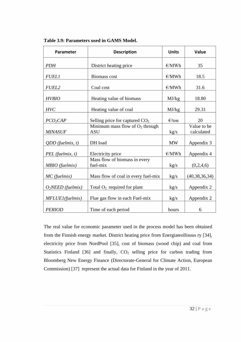
32 | P a g e
Table 3.9: Parameters used in GAMS Model.
Parameter Description Units Value
PDH District heating price €/MWh 35
FUEL1 Biomass cost €/MWh 18.5
FUEL2 Coal cost €/MWh 31.6
HVBIO Heating value of biomass MJ/kg 18.80
HVC Heating value of coal MJ/kg 29.31
PCO2CAP Selling price for captured CO2 €/ton 20
MINASUF
Minimum mass flow of O2 through
ASU kg/s
Value to be
calculated
QDD (fuelmix, t) DH load MW Appendix 3
PEL (fuelmix, t) Electricity price €/MWh Appendix 4
MBIO (fuelmix)
Mass flow of biomass in every
fuel-mix kg/s (0,2,4,6)
MC (fuelmix) Mass flow of coal in every fuel-mix kg/s (40,38,36,34)
O2NEED (fuelmix) Total O2 required for plant kg/s Appendix 2
MFLUE1(fuelmix) Flue gas flow in each Fuel-mix kg/s Appendix 2
PERIOD Time of each period hours 6
The real value for economic parameter used in the process model has been obtained
from the Finnish energy market. District heating price from Energiateollisuus ry [34],
electricity price from NordPool [35], cost of biomass (wood chip) and coal from
Statistics Finland [36] and finally, CO2 selling price for carbon trading from
Bloomberg New Energy Finance (Directorate-General for Climate Action, European
Commission) [37] represent the actual data for Finland in the year of 2011.

33 | P a g e
Positive variables in GAMS model have been shown in Table 3.10. These decision
variables have been declared with a statement and units.
Table 3.10: Positive variables in GAMS Model.
Positive variable Description Units
elnet(fuelmix,t) Electricity produced in power plant MW
elCO2comp(t) Electricity consumed in CO2 compression MW
elasu(t) Electricity consumed in ASU MW
elstg(t) Electricity consumed in Storage MW
m1O2asu(t) O2 flow out of ASU kg/s
m2O2asu(t) O2 flow out of ASU kg/s
mO2stgin(t) O2 flow into O2 storage kg/s
mO2stgout(t) O2 flow out from O2 storage kg/s
O2levstg(t) Level of O2 in storage kg/s
totO2(fuelmix,t) Total O2 need kg/s
3.3.2 Objective function
Objective function maximizes the profit in selling of electricity as well as buying of
fuel (fuel usage). Eq. (1) shows the structure of objective function that is denoted as
‘z’ and the corresponding equation has been illustrated as follows:
∑ ∑ (
) (1)

34 | P a g e
3.3.3 Equations for GAMS model
Equations in GAMS models require to be declaring and defining in the statement.
Equations are major power in the algebraic modeling language GAMS [33].
Eq. (2) shows the calculation for the power consumption in Air Separation Unit
(ASU) [11]:
(2)
Power consumption in carbon compression and purification unit (CPU) is expressed
by Eq. (3) [11]:
∑ ( )
(3)
Eq. (4) defines the power consumption in O2 storage and corresponding equation is as
follows:
(4)
Eqs. (4-8) represent power generation in every fuel mix (blend of coal and biomass)
( )
(5)
( )
(6)
( )
(7)
( )
(8)
35 | P a g e
Through the execution of GAMS Model, only one type of fuel mix for each period
was operated and Eq. (9) derives for the respective purpose.
∑ (9)
The mass flow of O2 required to the boiler for combustion of fuel is sum of the mass
of O2 from ASU to burner ( ) and O2 from storage ( ). Eq.
(10) defining the total oxygen requirement is as follows:
∑
(10)
Eq. (11) shows the mass of O2 from ASU splitting into two streams. For the better
optimization in GAMS Model, one O2 stream is denoted as O2 flow into storage
( ) and another stream as O2 from ASU to burner ( ).
(11)
The level of O2 in the storage system depends on time. To fit the equation, the
positive variables like O2 flow into storage ( ) and O2 from storage
( ) are considered. Eq. (12) defining the level of O2 in storage is
represented as follows:
( ) ( ) (12)
Usage of biomass in the process model has been limited. Eq. (13) for biomass usage
represents as:
∑ ∑( )
∑ ∑( ( ) ))
fuelmix FUELMIX, t T. (13)

36 | P a g e
3.3.4 Operational methodology of oxygen storage
Figure 3.4 demonstrates the overall operational methodology of O2 storage system for
proposed power plant. There should be two output lines from the ASU, one will
supply O2 directly to the boiler and another one connects the ASU with the O2 storage
facility. The control mechanism regarding the distribution of O2 in these two lines will
be entirely linked with grid electricity price. Suitable controllers and control strategy
will be adopted to execute the economical operation of ASU.
Figure 3.4: Overall system diagram including O2 storage with parameters and variables (based on Prosim and GAMS model parameters).

37 | P a g e
150
170
190
210
230
300.00 400.00 500.00 600.00
Ele
ctri
city
(M
W)
DH load (MW)
Fuel Mix 1
Fuel Mix 2
Fuel Mix 3
Fuel Mix 4
4 Results
4.1 Simulation results from process model
In this section, different curves have been developed to predict the behavior of
electricity and DH load for four design cases, built in Prosim by varying the following
two parameters:
(a) Fuel mix of coal and biomass
(b) District heating load.
4.1.1 Relation between DH and net electricity
These curves will provide a basis to optimize the plant from both technical and
economical point of view.
4.1.1.1 Design case 1: (Fuel mix 1 & DH load 90%)
Figure 4.1: Relation between DH load and net electricity for design case 1.

38 | P a g e
150
170
190
210
230
300.00 400.00 500.00 600.00
Ele
ctri
city
(M
W)
DH load (MW)
Fuel Mix 1
Fuel Mix 2
Fuel Mix 3
Fuel Mix 4
The design case 1 is prepared with fuel mix 1 (100% coal) and 90 % DH load. After
creating the design case 1, four types of fuel combination (fuel mix 1- 4), DH loads
(60-100%) are simulated on off-design mode in the design case. Figure 4.1 illustrates
that the behavior of electricity and DH load follows an inverse relation for all types of
fuel mix and at different DH loads. Therefore, it can be concluded that when DH load
increases, the electrical power from the plant decreases for all types of operating
condition.
4.1.1.2 Design case 2: (Fuel mix 4 & DH load 90%)
Like design case 1, the design case 2 is created from the same process model but
changing with fuel mix 2 (85% coal and 15% biomass) and 90 % DH load. Simulation
runs in off-design mode with changing the types of fuel combination and DH load.
The corresponding curve in Figure 4.2 is developed from the simulation results. In
Figure 4.2: Relation between DH load and net electricity for design case 2.
this case, the behavior of electricity and DH load follows an inverse relation with little
bit polynomial nature for all types of fuel mix and at different DH loads. The power
generation from design case 2 is less than design case 1 for all types of fuel mixes and
different DH load. For instance, the DH and electricity generation for design case 1

39 | P a g e
150
170
190
210
230
250
300.00 400.00 500.00 600.00
Ele
ctri
city
(M
W)
DH load (MW)
Fuel Mix 1
Fuel Mix 2
Fuel Mix 3
Fuel Mix 4
are 589.16 MWth and 197 MWe respectively (100% coal firing and 90% DH load)
while bit decreased value for design case 2 is shown as 584.59 MWth and 195.07
MWe respectively (same coal firing and DH load).
4.1.1.3 Design case 3: (Fuel mix 1 & DH load 70%)
The design parameter for case 3 is fuel mix 1 (100% coal firing) and 70 % DH load.
Running the simulation process is similar to design case 1 and 2. Fuel combination as
Fuel mix and DH load are simulated and the corresponding curve is shown in Figure
4.3.
Figure 4.3: Relation between DH load and net electricity for design case 3.
Figure 4.3 for design case 3 demonstrates the inverse behavior of electricity and DH
load for all types of fuel mix and different DH loads. Interestingly, the power
generation from this design case is almost equivalent to design case 1. The difference
between these two cases is the change in DH load. However, more electricity is
generated in design case 3 than design case 1 in case of fuel mixes (3-4). For example,
electricity generation in design case 1 and case 3 is 193.81 MWe and 195.71 MWe
respectively (for both case fuel mix 4 and DH load 60%) [Appendix: B]. However,

40 | P a g e
150
170
190
210
230
300.00 400.00 500.00 600.00
Ele
ctri
city
(M
W)
DH load (MW)
Fuel Mix 1
Fuel Mix 2
Fuel Mix 3
Fuel Mix 4
with the increase in DH load the electrical power from the plant decreases in all types
of operating condition.
4.1.1.4 Design case 4: (Fuel mix 4 & DH load 70%)
Figure 4.4: Relation between DH and net electricity for design case 4.
Fuel mix 4 (85% coal and 15% biomass) and 70 % DH load are key parameters to
construct the design case 4 in the process model. After simulating with different fuel
mixes and DH loads in off-design mode, the resultant data is shown as linear curve in
Figure 4.4. Like all three previous design cases, this case also demonstrates the
inverse behavior of electricity and DH load for all types of fuel mixes and different
DH loads. Higher electricity generation is observed in design case 4 compared to
design case 2 when the DH load is 60%-70%. In contrast, DH generation is bit higher
in design case 2 than in design case 1 for most of the fuel mixes.
The key target behind the development of four design cases for same parameters is to
suggest a best and optimized operational scenario for the plant. After a close analysis
of the curves, it can be concluded that the design case 3 offers maximum electrical
power for a certain DH load for all types of fuel mix.

41 | P a g e
0.500.530.560.590.620.650.680.710.740.770.800.83
0% 5% 10% 15% 20%
Ne
t e
ffic
ien
cy
Percentage of Biomass with coal (%)
DH load 100%
DH load 90%
DH load 80%
DH load 70%
DH load 60%
4.1.2 Net efficiency versus biomass percentage with coal
In the simulation of the process model, net efficiency refers to the combined
efficiency of net electrical power and useful heat for district heating. Moreover, the
net electricity is considered as the electricity available after electricity consumption
for all auxiliaries including ASU and CPU.
4.1.2.1 Design case 1: (Fuel mix 1 & DH load 90%)
In design case 1, the maximum efficiency was found in the operation at off- design
mode with DH load 90% and fuel mix 4. Efficiency value accounts for 76%.
However, running the model with DH load 60% and fuel mix 1 showed the minimum
net efficiency value of 56%. It is clearly observed that net efficiency increases with
adding the biomass portion to coal (Figure 4.5). Obviously, net efficiency is higher in
Fuel case 4 than rest of the type of mixture.
4.1.2.2 Design case 2: (Fuel mix 4 & DH load 90%)
Efficiency decreases by 1% in design case 2 (fuel Mix 4 and DH load 90%) regardless
changing DH load and fuel mix. Figure 4.6 represents the graph for design case 2.
Figure 4.5: Change of net efficiency with biomass percentage (design case 1).

42 | P a g e
0.500.530.560.590.620.650.680.710.740.770.800.83
0% 5% 10% 15% 20%
Ne
t e
ffic
ien
cy
Percentage of biomass with coal (%)
DH load 100%
DH load 90%
DH load 80%
DH load 70%
DH load 60%
0.500.530.560.590.620.650.680.710.740.770.800.83
0% 5% 10% 15% 20%
Ne
t e
ffic
ien
cy
Percentage biomass in coal (%)
DH load 100%
DH load 90%
DH load 80%
DH load 70%
DH load 60%
4.1.2.3 Design case 3: (Fuel mix 1 & DH load 70%)
Figure 4.7 for design case 3 illustrates the equivalence efficiency to design case 1.
Design case 3 also matches to design case 2 interim of efficiency to some extent.
Figure 4.6: Change of net efficiency with biomass percentage (design case 2).
Figure 4.7: Change of net efficiency with biomass percentage (design case 3).

43 | P a g e
0.500.530.560.590.620.650.680.710.740.770.800.83
0% 5% 10% 15% 20%
Ne
t e
ffic
ien
cy
Percentage of biomass in coal (%)
DH load 100%
DH load 90%
DH load 80%
DH load 70%
DH load 60%
4.1.2.4 Design case 4: (Fuel mix 4 & DH load 70%)
Design case 4 demonstrates the same trend of efficiency that other design cases have
shown. Figure 4.8 shows that net efficiency increases with more blending of biomass
like the other design cases. In this case, efficiency is close to the efficiency of design
case 2.
All the Figures show that there is an increase in net efficiency with the rise of biomass
percentage in co- firing with coal. The increasing amount of biomass percentage in
co-firing will cause a drop of fuel power which results in electrical power loss
because the DH is kept constant. Therefore, a drop of electrical power is favorable to
increase the net efficiency. Although the rate of increase of net efficiency (slope of
the lines are equal) is same in all DH cases, but the maximum efficiency will be
achieved in design case 1 and 3 (in both cases, same fuel mix 1 as design parameter,
but DH load is different). Replacing biomass with coal indicates a sense of
sustainability because of carbon neutral nature of biomass. The nature of the graphs
suggests that a sustainable operational mode of plant also results in the efficiency
increase.
Figure 4.8: Change of net efficiency with biomass percentage (design case 4).

44 | P a g e
72.00
74.00
76.00
78.00
80.00
82.00
84.00
86.00
0% 5% 10% 15% 20%
O2
mas
s fl
ow
(kg
/s)
Biomass percentage with coal (%)
Flue gas massflow
Theoretical concepts suggest that it is always economical to reduce the energy
conversion chain. In DH case, low-grade energy is used for generating heat thereby
reducing one-step in energy conversion. Consequently, it will always be better to use
most of the fuel power as heat rather than converting into electricity. Nevertheless, in
practical scenario there should be a balance between the utilization of heat and
electricity.
The rise of biomass percentages is closely related to the amount of electrical power
that can be compromised. Too much compromise on electrical power may not be
suitable for some particular cases in the grid. The mix of biomass in co-firing is
actually dependent on the grid electricity price and district heating price. A balanced
correlation needs to be developed to define the co-firing ratio.
4.1.3 O2 mass flow versus biomass percentage with coal
Figure 4.9 shows that the O2 requirement from ASU drops with the increase in
biomass percentage in the co-firing. From the chemical analysis of biomass, it is
found that the carbon content of biomass is less than coal. From the fuel analysis
(Table: 3.2), coal used in the process plant has 9.1% O2 (dry wt.%) whereas biomass
(wood chip) O2 value is 42.5% (dry wt.%). As the carbon content is less in biomass, it
Figure 4.9: Change of O2 stream with biomass percentage (all design cases).

45 | P a g e
is very natural that the oxygen will also drop in combustion. In the process model, O2
requirement was 93.65 kg/s in 100% coal input. Required O2 level decreases with
addition of biomass and it declined to 75 kg/s, when 15% biomass was added to
combust with 85% coal. Therefore, this graph encourages the co-firing of more
biomass with coal to reduce the power consumption of ASU.
4.2 Optimization results from GAMS model
4.2.1 Oxygen storage model
In the proposed power plant, ASU for the oxyfuel combustion is the biggest auxiliary
in the power plant. As a result, it will be interesting to investigate an economic
operational methodology of this high-energy consuming auxiliary equipment with the
help of GAMS optimization tools. To optimize the operational load of ASU, the
concept of oxygen storage is introduced based on grid electricity price.
In the optimization, Finnish electricity price from NordPool has been taken as
reference to link the feasibility of oxygen storage with electricity price. The control or
operational methodology for the ASU is as follows:
(a) When the grid electricity price is low then it is advisable to operate the ASU at
its maximum capacity, so that a certain amount of oxygen can be stored apart
from fulfilling the boiler demand.
(b) The stored oxygen can be used during high grid electricity price.
(c) Suitable control strategy should be adopted to sense the grid electricity price
and execute the ASU operation economically.
The market price of electricity for the 2011 taken from NordPool is simulated in
GAMS model to develop the yearly trend [35]. The data has been taken at an interval
of six hours for the whole year of 2011. The oxygen requirement for the oxyfuel
combustion is optimized in GAMS based on the model developed in Prosim 5.6.
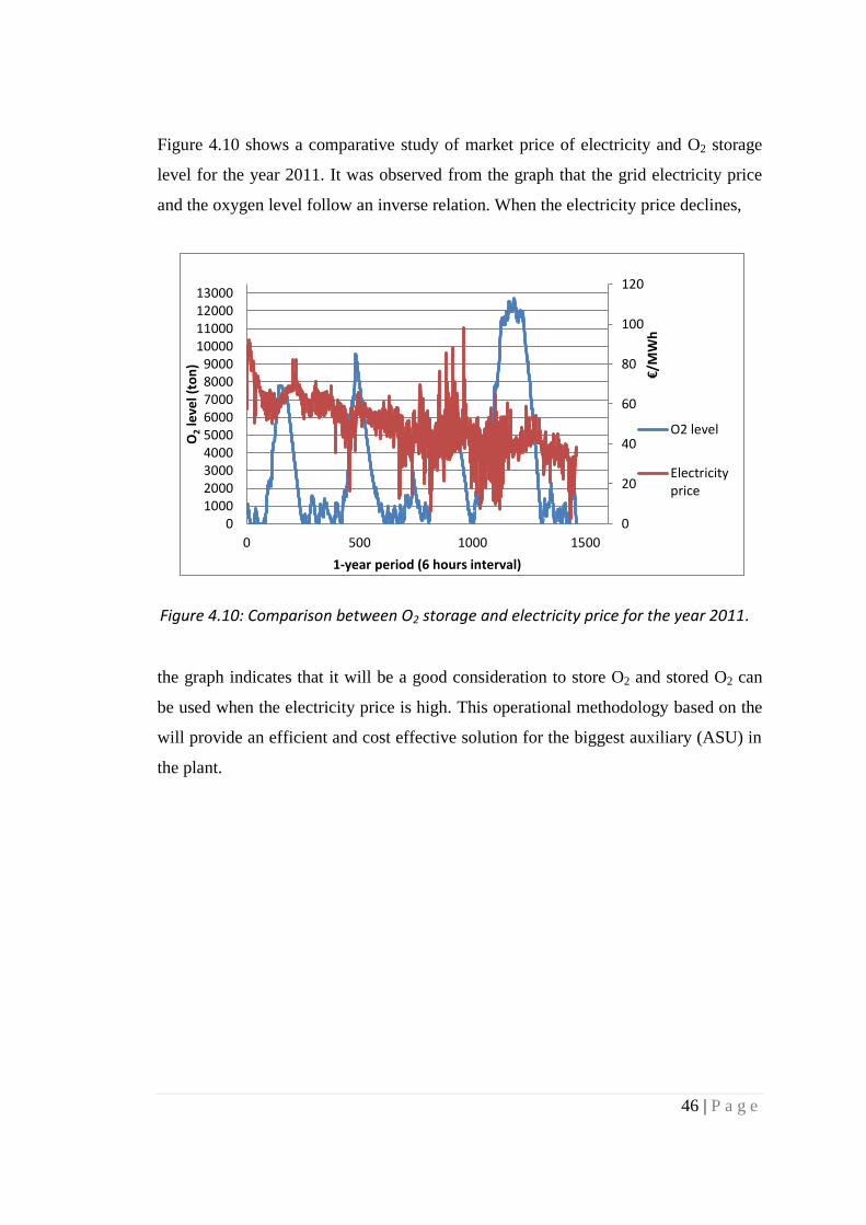
46 | P a g e
0
20
40
60
80
100
120
0100020003000400050006000700080009000
10000110001200013000
0 500 1000 1500
O2
leve
l (to
n)
1-year period (6 hours interval)
O2 level
Electricityprice
€/M
Wh
Figure 4.10 shows a comparative study of market price of electricity and O2 storage
level for the year 2011. It was observed from the graph that the grid electricity price
and the oxygen level follow an inverse relation. When the electricity price declines,
the graph indicates that it will be a good consideration to store O2 and stored O2 can
be used when the electricity price is high. This operational methodology based on the
will provide an efficient and cost effective solution for the biggest auxiliary (ASU) in
the plant.
Figure 4.10: Comparison between O2 storage and electricity price for the year 2011.

47 | P a g e
4.2.2 Economic evaluation considering O2 storage
In the thesis work, the economic evaluation has not been analyzed in detail. For the
optimization of O2 storage, the key economic parameters includes the cost of fuel
(coal and biomass), market electricity price, district heating price and selling price of
captured CO2 for carbon trading. All the economic data have been taken from Finnish
market value for the year 2011 (Table 4.1).
From the optimization of the process model with O2 storage system, positive value
has been derived. However, investment cost and maintenance cost were not
considered. It was preliminary assumed that positive value would indicate feasibility
of the plant with storage system, otherwise it will not be suggested to use O2 storage
system in case of negative value.
Table 4.1: Economic data used for process model.
Description Units Value References
District heating price €/MWh 35 [34]
Electricity price €/MWh Appendix D [35]
Cost of biomass (Forest chips) €/MWh 18.5 [36]
Cost of coal €/MWh 31.6 [36]
Price for selling captured CO2 €/ton 20 [37]
Table 4.2: O2 storage benefit potential for all design cases.
Design cases With
Storage (€) Without Storage(€)
Storage benefit potential (€)
Design case 1 3,038,951,000 2,959,353,000 79,598,000
Design case 2 3,036,412,000 2,956,806,000 79,606,000
Design case 3 3,039,524,000 2,959,927,000 79,597,000
Design case 4 3,037,718,000 2,958,559,000 79,159,000

48 | P a g e
From Table 4.2, it is clearly observed the positive value for storage of O2 in all design
cases. Among all four design cases, design case 3 (100% coal and DH load 70%)
indicates high profit from the process model considering Finnish market electricity
price and average value for district heating price for the year 2011.
The price for CO2 trading under EU Emission Trending Scheme (EU ETS) ranges
from 20 €/ton to 25 €/ton (projection year 2020-30 with real data of 2009), 16 €/ton.
In this process model, the assumption for CO2 price is 20 €/ton [37]. The higher price
for CO2 trading and district heating price will lead the profit in the proposed power
plant. In contrast, different prices are fixed in the market for district heating for
different European countries. Even, a wide range of DH price (€/MWh) has been
offered by DH wholesalers in the Finnish district heating market. In this research
work, the value for DH selling price is 35 €/MWh [34]. When the value rises, the
profit will gradually increase. Furthermore, there might be chance to purchase
electricity from the Nordic electricity market. In contrary, DH system is particularly
dependent inside the country with characteristic of local market strategy.

49 | P a g e
5 Discussion
The proposed model of the power plant is simulated in Prosim 5.6 for different design
cases by varying the fuel mix and DH load. The different design cases will analyze
the feasibility of oxyfuel combustion, flue gas recirculation, district heating, O2
storage and carbon capture for the proposed power plant. The state of art technology
suggests the feasibility of oxyfuel combustion with carbon capture, but there is no
explanation of reducing the energy consumption of ASU and a provision to use the
waste heat.
Keeping the background problem in mind, this research work has focused on
available state of art technologies related to carbon capture along with the
incorporation of different variables that may be beneficial for efficiency and
economic justification.
Oxyfuel combustion along with flue gas recirculation is an important issue related to
carbon capture. For the oxyfuel combustion, it is necessary to separate pure O2 from
air in a highly inefficient air separation unit. In the analysis, a special attention is
given to address the high-energy consumption problem of ASU. The design of
suitable burners for oxyfuel combustion is an important matter that needs to be
developed more in the future for commercial use. All the plants are still in
demonstration stage. The portion of flue gas recirculation is 70 %, as many research
projects have used this value in a better way. Although it is also possible to optimize
that amount, but it seems to be quite difficult with the present scope of this thesis
work. Therefore, a standard value of 70% for the flue gas recirculation amount has
been taken after proper literature review.
The district heating concept is one of the key features in this thesis. From economic
and efficiency perspective, it is a good impression to use the waste heat from the
power plant into district heating system. Relevant curves and data are developed to
justify the use of CHP plant for the proposed design. Furthermore, the results show a

50 | P a g e
good commercial justification for the increase in district heating load by
compromising on electrical power. There is an interesting phenomenon be considered
that increase in biomass in co-firing results in a rise in net efficiency.
Due to highly inefficient ASU unit, a promising concept of O2 storage is developed
through this research work. The operational strategy of O2 storage is linked with the
grid electricity price. The feasibility of this concept is clearly explained in the thesis
by proper scientific calculation and curves. The data for this analysis is taken from
Statistics Finland and Finnish energy market for the year 2011. Therefore, the idea of
O2 storage is well explained with real data and can be used for actual
implementations.
A total investigation has been done on the whole process to integrate and properly
optimize the proposed design in a scientific way with commercial justification.

51 | P a g e
6 Conclusion
In the upcoming years, coal will be a dominant source of energy. Although renewable
energy technologies will play an important role to meet the energy demand by
environmental friendly methods. However, renewable energy is still facing problems
for complete commercialization due to financial and technological constraints. These
issues will bring opportunities forward to develop a research field to generate clean
energy from coal by CCS.
In this thesis, process modeling and optimization have been executed for a co-firing
CHP power plant with a facility of carbon capture. The model of the proposed power
plant has been created in Prosim 5.6 with the help of suitable tools. For the
optimization part, a separate code with statements has written in GAMS programme
based on Prosim model. After creating the model, a set of variables have been
selected to define the optimization results. The variables are as follows:
(a) Co-firing of coal with biomass
(b) 70% recirculation of flue gas
(c) District heating
(d) O2 storage concept linked with grid electricity price
(e) Carbon capture and storage.
The proposed model in Prosim 5.6 and its corresponding optimization routine in
GAMS model provide us a number of important conclusions that are worth noting and
listed as follows:
There is a linear co-relation between the biomass percentage in co-firing and
the net efficiency. The results show a 4-5 % increase in net efficiency with the rise of
biomass percentage from 5% to 15 % in co-firing. Therefore, this result justifies the
co-firing of coal with biomass concerning net efficiency.
There is another important conclusion to be considered that the effect of
biomass percentage on oxygen requirement of boiler. With the rise of biomass

52 | P a g e
percentage in co-firing from 0 to 15%, the oxygen requirement of the boiler reduces
from 83 kg/s to 75 kg/s, because carbon content is less in biomass than coal and
decreasing the coal amount (from 100% to 85%) leads the less requirement of O2 from
ASU. Actually, this incident will reduce the power consumption of ASU, which is
good for the overall efficiency of a power plant. Therefore, it can be concluded in this
context that an increase in overall efficiency of plant can be possible with increase of
biomass percentage.
The concept of O2 storage introduced in the work will drastically increase the
economic efficiency of ASU. The main challenge for oxyfuel combustion is the high
power consumption of ASU. If the consumption is reduced then the results and
analysis are very relevant and important to the research field of carbon capture.
Furthermore, using cheap grid electricity for O2 separation and stored O2 for usage
during high grid electricity price makes sense for the economy of ASU operation.
An analysis of heat and power ratio for the CHP plant indicates positive effect
during high district heating price. In this thesis, a feasibility analysis with suitable
graphs has been conducted to link the variation of heat and power ratio with the grid
electricity and district heating price.
By combining the above variables, different design conditions are created in GAMS
model for the optimization of the proposed power plant. The design cases reflect the
optimized operational scenario that might be very useful for a real power plant. The
results will provide a solution for a power plant to modify and optimize their power
plant towards the goal of sustainability.
In future, fossil fuel price will be increased. More carbon tax will be imposed as well.
As a result, many power generation companies will switch to renewable energy
sources. Moreover, they will also focus on increasing efficiency in existing
conventional power plants. Biomass based oxyfuel combustion and carbon capture
system is one of the best options for reducing greenhouse gases. It will help not only
in cutting the amount of CO2 but in also emphasizing the renewable energy sources
for better environment. The implementation of carbon capture technologies in coal-

53 | P a g e
based power plant has significant contribution on GHG emission all over the world.
The main driver of biomass based oxyfuel combustion technology is zero emissions
CO2 and near zero for pollutant including NOx, SOx and particulates.
6.1 Future work
It has been explained that coal will dominate the fuel trend to be used for power
generation next couple of decades. Consistent supply, relatively cheap price and
availability in most parts of the world have enabled this fossil fuel to take a lead. No
doubt, carbon capture and storage will be a leading contributor for reduction of CO2
emissions. Moreover, oxyfuel combustion with CCS has the chance to be an attractive
technology for the declination of greenhouse gases.
Through this thesis, it has been tried to incorporate together some approaches, such as
fuel flexibility by blending coal and biomass, CHP plant for cogeneration concept,
using CFB boiler in oxyfuel combustion, CCS system and finally O2 storage system.
These approaches mentioned before have different characteristic with merits and
demerits as well. Many researchers and organizations are working collaboratively in
this field. All the plants are still in pilot project and demonstration mode. In near
future, we will observe the significant development in this CO2 mitigation field.
During this thesis with modeling of the proposed plant, some features came forward
to be considered in the future. These several features are mentioned as follows:
ASU and CPU consume large percentage of the gross power thus decreasing
overall efficiency. More research works is essential for a more efficient
system.
The combustion characteristic inside the boiler is an important issue. High
pure O2 with RFG (CO2-H2O) has complex characteristics, as combustion
atmosphere is quite different in oxyfuel combustion in comparison to
conventional power plant. The characteristics like ignition temperature, heat
54 | P a g e
transfer, pollution formation needs more experimental works for better
performance.
Blend of biomass with coal and their combustion behavior and ash properties
requires more investigation.
Effect of higher flame temperature and different combustion situations may
affect the boiler life. These issues require more evaluation.
As the O2 storage system in oxyfuel combustion and CCS is relatively new,
intensive research work is essential for optimization of storage system and
pricing of electricity and DH.

55 | P a g e
References
[1] M. B. Toftegaard, J. Brix, P. A. Jensen, P. Glarborg, and A. D. Jensen, "Oxy-
fuel combustion of solid fuels," Progress in Energy and Combustion Science,
vol. 36, no. 5, pp. 581-625, 2010.
[2] International Energy Agency (IEA), "CO2 Capture and Storage: A key carbon
abatement option," IEA Publication, Paris, 2008 [Online]. Available:
http://www.iea.org/textbase/nppdf/free/2008/CCS_2008.pdf. [Accessed:
March 10, 2012].
[3] J. Riaza, M. V. Gil, L. Álvarez, C. Pevida, J. J. Pis, and F. Rubiera, "Oxy-fuel
combustion of coal and biomass blends," Energy, vol. 41, no. 1, pp. 429-435,
2012.
[4] U.S. Energy Information Administration (EIA), "International Energy Outlook
2011," U.S. Energy Information Administration, Washington, DC, DOE/EIA-
0484(2011), 2011 [Online]. Available:
http://www.eia.gov/forecasts/ieo/pdf/0484(2011).pdf. [Accessed: March 29,
2012].
[5] International Energy Agency (IEA), "Energy Technology perspective 2010-
Scenarioes & Strategies to 2050," International Energy Agency (IEA), IEA
Publications, Paris, 2010 [Online]. Available:
http://www.iea.org/Textbase/nppdf/free/2010/etp2010_part1.pdf. [Accessed:
March 14, 2012].
[6] T. F. Wall, "Combustion processes for carbon capture," Proceedings of the
Combustion Institute, vol. 31, no. 1, pp. 31-47, 2007.
[7] B. Arias, C. Pevida, F. Rubiera, and J. J. Pis, "Effect of biomass blending on
coal ignition and burnout during oxy-fuel combustion," Fuel, vol. 87, no. 12,
pp. 2753-2759, 2008.
[8] L. Chen, S. Z. Yong, and A. F. Ghoniem, "Oxy-fuel combustion of pulverized
coal: Characterization, fundamentals, stabilization and CFD modeling,"
Progress in Energy and Combustion Science, vol. 38, no. 2, pp. 156-214,
2012.
[9] G. Scheffknecht, L. Al-Makhadmeh, U. Schnell, and J. Maier, "Oxy-fuel coal
combustion - A review of the current state-of-the-art," International Journal of
Greenhouse Gas Control, vol. 5, no. 3, pp. S16-S35, 2011.
56 | P a g e
[10] P. S. Pak, Y. D. Lee, and K. Y. Ahn, "Characteristics and economic evaluation
of a power plant applying oxy-fuel combustion to increase power output and
decrease CO2 emission," Energy, vol. 35, no. 8, pp. 3230-3238, 2010.
[11] E. S. Rubin, A. B. Rao, and M. B. Berkenpas, "Technical Documentation:
Oxygen-based Combustion Systems (Oxyfuels) with Carbon Capture and
Storage (CCS)," Department of Engineering and Public Policy, Carnegie
Mellon University, Pittsburgh, PA, Rep. 75, 2007 [Online]. Available:
http://repository.cmu.edu/epp/75. [Accessed: April 17, 2012].
[12] T. Wall and J. Yu, "Coal-fired oxyfuel technology status and progress to
deployment," in 34th International Technical Conference on Clean Coal &
Fuel Systems, Clearwater, FL, 2009. Available:
http://hdl.handle.net/1959.13/919253. [Accessed: February 26, 2012].
[13] H. Liu, R. Zailani, and B. M. Gibbs, "Pulverized coal combustion in air and in
O2/CO2 mixtures with NOx recycle," Fuel, vol. 84, no. 16, pp. 2109-2115,
2005.
[14] R. Viskanta, Radiative Transfer of Combustion Systems: Fundamentals and
Applications. New York: Begell House, 2005.
[15] B. J. P. Buhre, L. K. Elliott, C. D. Sheng, R. P. Gupta, and T. F. Wall, "Oxy-
fuel combustion technology for coal-fired power generation," Progress in
Energy and Combustion Science, vol. 31, no. 4, pp. 283-307, 2005.
[16] J. Koppejan and S. V. Loo, The Handbook of Biomass Combustion and Co-
firing. London, United Kingdom: Taylor & Francis, 2008.
[17] N. S. Yuzbasi and N. Selçuk, "Air and oxy-fuel combustion characteristics of
biomass/lignite blends in TGA-FTIR," Fuel Processing Technology, vol. 92,
no. 5, pp. 1101-1108, 2011.
[18] J. Zactruba. (2009). How does a Circulating Fluidized Bed Boiler Work ?
[Online]. Available: http://www.brighthubengineering.com/power-
plants/26547-how-does-a-circulating-fluidized-bed-boiler-work/. [Accessed:
May 20, 2012].
[19] Global Climate & Energy Project (GCEP), "An Assessment of Biomass
Feedstock and Conversion Research Opportunities," Global Climate & Energy
Project (GCEP), Stanford University, CA, 2005 [Online]. Available:
http://gcep.stanford.edu/pdfs/assessments/biomass_assessment.pdf. [Accessed:
June 29, 2012].

57 | P a g e
[20] D. Ciolkosz, "Renewable and Alternative Fact Sheet: Co-firing Biomass with
Coal," Ag Communications and Marketing, The Pennsylvania State
University, PA, 2010 [Online]. Available:
http://pubs.cas.psu.edu/FreePubs/PDFs/ub044.pdf. [Accessed: June 25, 2012].
[21] International Energy Agency (IEA), "Combined Heat and Power- Evaluating
the benefits of greater global investment," International Energy Agency (IEA),
Paris, France, 2008 [Online]. Available:
http://www.iea.org/papers/2008/chp_report.pdf. [Accessed: March 23, 2012].
[22] Energy Charter Secretariat, "Cogeneration and District Heating- Best Practices
for Municipalities," Brussels, Belgium, D/2005/7850/5, 2005 [Online].
Available: http://www.localpower.org/documents/reporto_ench_chp-dh.pdf.
[Accessed: April 02, 2012].
[23] EURELECTRIC, "European Combined Heat & Power: A Technical Analysis
of Possible Definition of the Concept of “Quality CHP”," Union of the
Electricity Industry (EURELECTRIC), Brussels, Belgium, Ref: 2002-112-
0004, 2002 [Online]. [Accessed: March 12, 2012].
[24] M. Danestig, A. Gebremehdin, and B. Karlsson, "Stockholm CHP potential-
An opportunity for CO2 reductions?," Energy Policy, vol. 35, no. 9, pp. 4650-
4660, 2007.
[25] K. Difs, "District Heating and CHP- Local Possibilites for global climate
change mitigation," Ph.D. dissertation, Department of Management and
Engineering, Linköping University, Linköping, Sweden, 2010.
[26] A. Aspelund and K. Jordal, "Gas conditioning—The interface between CO2
capture and transport," International Journal of Greenhouse Gas Control
vol. 1, no. 3, pp. 343-354, 2007.
[27] Endat Oy, Prosim Module reference manual, Endat Oy, Espoo, Finland, 2007.
[28] Y. Hu, "CO2 capture from oxyfuel combustion power plants," Licentiate
thesis, Dept. Chem. & Tech. , KTH Royal of Technology, Stockholm,
Sweden, 2011.
[29] J. Hong, G. Chaudhry, J. G. Brisson, R. Field, M. Gazzino, and A. F.
Ghoniem, "Analysis of oxy-fuel combustion power cycle utilizing a
pressurized coal combustor," Energy, vol. 34, no. 9, pp. 1332-1340, 2009.
[30] A. Seltzer, Z. Fan, and H. Hack, "Oxyfuel Coal Combustion Power Plant
System Optimization," in 7th Annual COAL-GEN Conference, Milwaukee,
WI, 2007 Available:
http://www.fwc.com/publications/tech_papers/files/TP_CCS_07_03.pdf.
[Accessed: July 30, 2012].

58 | P a g e
[31] L. Pirhonen, "Effects of Carbon Capture on a Combined Cycle Gas Turbine,"
M.S. thesis, Dept. Ind. Eng. & Manage., Tampere University of Technology,
Tampere, Finland, 2011.
[32] H. Mirzaesmaeeli, A. Elkamel, P. L. Douglas, E. Croiset, and M. Gupta, "A
multi-period optimization model for energy planning with CO2 emission
consideration," J Environ Manage, vol. 91, no. 5, pp. 1063-1070, 2010.
[33] R. E. Rosenthal. (2012). A GAMS Tutorial [Online]. Available:
http://www.gams.com/dd/docs/gams/Tutorial.pdf. [Accessed: April 23, 2012].
[34] Energiateollisuus ry, "District heating prices, type of houses in different
localities: District heating Prices 07/01/2011," Helsinki, Finland, 2012
[Online]. Available: http://energia.fi/tilastot/kaukolammon-hinnat-
tyyppitaloissa-eri-paikkakunnilla. [Accessed: August 1, 2012].
[35] Nord Pool Spot. (2012). Elspot prices [Online]. Available:
http://www.nordpoolspot.com/Market-data1/Elspot/Area-
Prices/ALL1/Hourly/. [Accessed: June 4, 2012].
[36] Official Statistics of Finland (OSF), "Energy prices," Helsinki: Statistics
Finland, ISSN=1799-800X, 2011 [Online]. Available:
http://www.stat.fi/til/ehi/2011/01/ehi_2011_01_2011-06-22_en.pdf.
[Accessed: June 25, 2012].
[37] Bloomberg New Energy Finance, "Emission performance Standards: Impacts
of power plant CO2 emission performance standards in the context of the
European carbon market " The Directorate-General for Climate Action,
Euroepan Commission, 2011 [Online]. Available:
http://ec.europa.eu/clima/policies/lowcarbon/ccs/docs/impacts_en.pdf.
[Accessed: July 24, 2012].
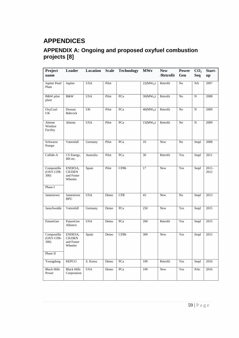
59 | P a g e
APPENDICES
APPENDIX A: Ongoing and proposed oxyfuel combustion projects [8]
Project
name
Leader Location Scale Technology MWe New
/Retrofit
Power
Gen
CO2
Seq
Start-
up
Jupiter Pearl
Plant
Jupiter USA Pilot 22(MWth) Retrofit No NA 2007
B&W pilot
plant
B&W USA Pilot PCa 30(MWth) Retrofit No N 2008
OxyCoal-
UK
Doosan
Babcock
UK Pilot PCa 40(MWth) Retrofit No N 2009
Alstom
Windsor
Facility
Alstom USA Pilot PCa 15(MWth) Retrofit No N 2009
Schwarze
Pumpe
Vattenfall Germany Pilot PCa 10 New No Seqd 2008
Callide-A CS Energy,
IHI etc.
Australia Pilot PCa 30 Retrofit Yes Seqd 2011
Compostilla
(OXY-CFB-300)
ENDESA,
CIUDEN and Foster
Wheeler
Spain Pilot CFBb 17 New Yes Seqd 2011–
2012
Phase I
Jamestown Jamestown
BPU
USA Demo CFB 43 New No Seqd 2013
Janschwalde Vattenfall Germany Demo PCa 250 New Yes Seqd 2015
FutureGen FutureGen
Alliance
USA Demo PCa 200 Retrofit Yes Seqd 2015
Compostilla
(OXY-CFB-300)
ENDESA,
CIUDEN and Foster
Wheeler
Spain Demo CFBb 300 New Yes Seqd 2015
Phase II
Youngdong KEPCO S. Korea Demo PCa 100 Retrofit Yes Seqd 2016
Black Hills
Power
Black Hills
Corporation
USA Demo PCa 100 New Yes NAc 2016

60 | P a g e
APPENDIX B: Simulation results for all design cases
Design Case 1: (Fuel mix 1 & DH 90%)
Parameter Unit Fuel mix 1 Fuel mix 2 Fuel mix 3 Fuel mix 4
Fuel flow
Coal kg/s 40 38 36 34
Biomass kg/s 0 2 4 6
Oxygen mass flow kg/s 83.65 80.76 77.88 75.00
Flue gas mass flow kg/s 413.48 404.03 394.57 385.11
Flue gas temperature inlet to Boiler °C 1861.93 1829.75 1796.19 1761.38
Flue gas mass flow for capture kg/s 106.62 103.09 99.95 96.01
Gas analysis (%)
N2
6.10 6.09 6.08 6.07
H2O
3.17 3.17 3.17 3.17
CO2
87.23 87.25 87.27 87.29
O2
3.02 3.01 3.01 3.01
SO2
0.45 0.44 0.43 0.42
Steam flow for 100% DH Load kg/s 280.00 280.00 280.00 280.00
DH load MW 589.16 590.26 590.06 593.33
Gross power MW 311.01 296.47 283.32 266.15
ASU MW 63.84 61.64 59.44 57.24
CPU MW 49.89 48.25 46.79 44.95
Net power MW 197.28 186.58 177.09 163.96
Fuel power MW 1039.32 1001.52 963.72 925.92
Electrical efficiency
0.19 0.19 0.18 0.18
Net efficiency (DH & net power)
0.76 0.78 0.80 0.82
Power to heat ratio
0.33 0.32 0.30 0.28
DH Temperature °C 100 100 100 100
Parameter Unit Fuel mix 1 Fuel mix 2 Fuel mix 3 Fuel mix 4
Fuel flow
Coal kg/s 40 38 36 34
Biomass kg/s 0 2 4 6
Oxygen mass flow kg/s 83.65 80.76 77.88 75.00
Flue gas mass flow kg/s 413.48 404.03 394.57 385.11
Flue gas temperature inlet to Boiler °C 1861.87 1829.69 1796.12 1761.32
Flue gas mass flow for capture kg/s 106.62 103.09 99.55 96.01
Gas analysis (%)
N2
6.10 6.09 6.08 6.07
H2O
3.17 3.17 3.17 3.17
CO2
87.23 87.25 87.27 87.29
O2
3.02 3.01 3.01 3.00
SO2
0.45 0.44 0.43 0.42
Steam flow for 90% DH Load kg/s 252.00 252.00 252.00 252.00
DH load MW 530.28 531.26 531.08 534.06
Gross Power MW 318.36 304.15 291.31 274.43
ASU MW 63.84 61.64 59.44 57.24
CPU MW 49.89 48.25 46.79 44.95
Net power MW 204.63 194.26 185.08 172.24
Fuel power MW 1039.32 1001.52 963.72 925.92
Electrical efficiency
0.20 0.19 0.19 0.19
Net efficiency (DH & net power)
0.71 0.72 0.74 0.76
Power to heat ratio
0.39 0.37 0.35 0.32
DH Temperature °C 100 100 100 100

61 | P a g e
Parameter Unit Fuel mix 1 Fuel mix 2 Fuel mix 3 Fuel mix 4
Fuel flow
Coal kg/s 40 38 36 34
Biomass kg/s 0 2 4 6
Oxygen mass flow kg/s 83.65 80.76 77.88 75.00
Flue gas mass flow kg/s 413.48 404.03 394.57 385.11
Flue gas temperature inlet to Boiler °C 1861.81 1829.62 1796.07 1761.25
Flue gas mass flow for capture kg/s 106.62 103.09 99.55 96.01
Gas analysis (%)
N2
6.10 6.09 6.08 6.07
H2O
3.17 3.17 3.17 3.17
CO2
87.23 87.25 87.27 87.29
O2
3.02 3.01 3.01 3.00
SO2
0.45 0.44 0.43 0.42
Steam flow for 80% DH Load kg/s 224.00 224.00 224.00 224.00
DH load MW 471.40 472.25 472.10 474.78
Gross power MW 325.22 311.31 298.72 282.13
ASU MW 63.84 61.64 59.44 57.24
CPU MW 49.89 48.25 46.79 44.95
Net power MW 211.49 201.42 192.49 179.94
Fuel power MW 1039.32 1001.52 963.72 925.92
Electrical efficiency
0.20 0.20 0.20 0.19
Net efficiency (DH & net power)
0.66 0.67 0.69 0.71
Power to heat ratio
0.45 0.43 0.41 0.38
DH Temperature °C 100 100 100 100
Parameter Unit Fuel mix 1 Fuel mix 2 Fuel mix 3 Fuel mix 4
Fuel flow
Coal kg/s 40 38 36 34
Biomass kg/s 0 2 4 6
Oxygen mass flow kg/s 83.65 80.76 77.88 75.00
Flue gas mass flow kg/s 413.48 404.03 394.57 385.11
Flue gas temperature inlet to Boiler °C 1861.76 1829.57 1796.01 1761.19
Flue gas mass flow for capture kg/s 106.62 103.09 99.55 96.01
Gas analysis (%)
N2
6.10 6.09 6.08 6.07
H2O
3.17 3.17 3.17 3.17
CO2
87.23 87.25 87.27 87.29
O2
3.02 3.01 3.01 3.00
SO2
0.45 0.44 0.43 0.42
Steam flow for 70% DH Load kg/s 196.00 196.00 196.00 196.00
DH load MW 412.50 413.24 413.13 415.48
Gross power MW 331.56 317.95 305.59 289.33
ASU MW 63.84 61.64 59.44 57.24
CPU MW 49.89 48.25 46.79 44.95
Net power MW 217.83 208.06 199.36 187.14
Fuel power MW 1039.32 1001.52 963.72 925.92
Electrical efficiency
0.21 0.21 0.21 0.20
Net efficiency (DH & net power)
0.61 0.62 0.64 0.65
Power to heat ratio
0.53 0.50 0.48 0.45
DH Temperature °C 100 100 100 100

62 | P a g e
Parameter Unit Fuel mix 1 Fuel mix 2 Fuel mix 3 Fuel mix 4
Fuel flow
Coal kg/s 40 38 36 34
Biomass kg/s 0 2 4 6
Oxygen mass flow kg/s 83.65 80.76 77.88 75.00
Flue gas mass flow kg/s 413.48 404.03 394.57 385.11
Flue gas temperature inlet to Boiler °C 1861.71 1829.52 1795.95 1761.14
Flue gas mass flow for capture kg/s 106.62 103.09 99.55 96.01
Gas analysis (%)
N2
6.10 6.09 6.08 6.07
H2O
3.17 3.17 3.17 3.17
CO2
87.23 87.25 87.27 87.29
O2
3.02 3.01 3.01 3.00
SO2
0.45 0.44 0.43 0.42
Steam flow for 60% DH Load kg/s 168.00 168.00 168.00 168.00
DH load MW 353.60 354.22 354.15 356.17
Gross power MW 337.37 324.07 311.94 296.00
ASU MW 63.84 61.64 59.44 57.24
CPU MW 49.89 48.25 46.79 44.95
Net power MW 223.64 214.18 205.71 193.81
Fuel power MW 1039.32 1001.52 963.72 925.92
Electrical efficiency
0.22 0.21 0.21 0.21
Net efficiency (DH & net power)
0.56 0.57 0.58 0.59
Power to heat ratio
0.63 0.60 0.58 0.54
DH Temperature °C 100 100 100 100

63 | P a g e
Design case 2: (Fuel mix 4 & DH 90%)
Parameter Unit Fuel mix 1 Fuel mix 2 Fuel mix 3 Fuel mix 4
Fuel flow
Coal kg/s 40 38 36 34
Biomass kg/s 0 2 4 6
Oxygen mass flow kg/s 83.65 80.76 77.88 75.00
Flue gas mass flow kg/s 413.48 404.03 394.57 385.11
Flue gas temperature inlet to Boiler °C 1862.55 1830.28 1796.59 1761.51
Flue gas mass flow for capture kg/s 106.62 103.09 99.55 96.01
Gas analysis (%)
N2
6.10 6.09 6.08 6.07
H2O
3.17 3.17 3.17 3.07
CO2
87.23 87.25 87.27 87.29
O2
3.02 3.01 3.01 3.00
SO2
0.45 0.44 0.43 0.42
Steam flow for 100% DH Load kg/s 280 280 280 280
DH load MW 584.59 587.23 587.85 588.42
Gross power MW 308.80 293.12 279.68 266.12
ASU MW 63.84 61.64 59.44 57.24
CPU MW 49.89 48.25 46.79 44.95
Net power MW 195.07 183.23 173.45 163.93
Fuel power MW 1039.32 1001.52 963.72 925.92
Electrical efficiency
0.19 0.18 0.18 0.18
Net efficiency (DH & net power)
0.75 0.77 0.79 0.81
Power to heat ratio
0.33 0.31 0.30 0.28
DH Temperature °C 100 100 100 100
Parameter Unit Fuel mix 1 Fuel mix 2 Fuel mix 3 Fuel mix 4
Fuel flow
Coal kg/s 40 38 36 34
Biomass kg/s 0 2 4 6
Oxygen mass flow kg/s 83.65 80.76 77.88 75.00
Flue gas mass flow kg/s 413.48 404.03 394.57 385.11
Flue gas temperature inlet to Boiler °C 1862.50 1830.22 1796.53 1761.44
Flue gas mass flow for capture kg/s 106.62 103.09 99.55 96.01
Gas analysis (%)
N2
6.10 6.09 6.08 6.07
H2O
3.17 3.17 3.17 3.07
CO2
87.23 87.25 87.27 87.29
O2
3.02 3.01 3.01 3.00
SO2
0.45 0.44 0.43 0.42
Steam flow for 90% DH Load kg/s 252.00 252.00 252.00 252.00
DH load MW 526.60 528.96 529.54 530.06
Gross power MW 314.75 299.62 286.74 273.71
ASU MW 63.84 61.64 59.44 57.24
CPU MW 49.89 48.25 46.79 44.95
Net power MW 201.02 189.73 180.51 171.52
Fuel power MW 1039.32 1001.52 963.72 925.92
Electrical efficiency
0.19 0.19 0.19 0.19
Net efficiency (DH & net power)
0.70 0.72 0.74 0.76
Power to heat ratio
0.38 0.36 0.34 0.32
DH Temperature °C 100 100 100 100

64 | P a g e
Parameter Unit Fuel mix 1 Fuel mix 2 Fuel mix 3 Fuel mix 4
Fuel flow
Coal kg/s 40 38 36 34
Biomass kg/s 0 2 4 6
Oxygen mass flow kg/s 83.65 80.76 77.88 75.00
Flue gas mass flow kg/s 413.48 404.03 394.57 385.11
Flue gas temperature inlet to Boiler °C 1862.46 1830.17 1796.47 1761.38
Flue gas mass flow for capture kg/s 106.62 103.09 99.55 96.01
Gas analysis (%)
N2
6.10 6.09 6.08 6.07
H2O
3.17 3.17 3.17 3.07
CO2
87.23 87.25 87.27 87.29
O2
3.02 3.01 3.01 3.00
SO2
0.45 0.44 0.43 0.42
Steam flow for 80% DH Load kg/s 224.00 224.00 224.00 224.00
DH load MW 468.51 470.59 471.15 471.61
Gross power MW 319.67 305.12 292.71 280.19
ASU MW 63.84 61.64 59.44 57.24
CPU MW 49.89 48.25 46.79 44.95
Net power MW 205.94 195.23 186.48 178.00
Fuel power MW 1039.32 1001.52 963.72 925.92
Electrical efficiency
0.20 0.19 0.19 0.19
Net efficiency (DH & net power)
0.65 0.66 0.68 0.70
Power to heat ratio
0.44 0.41 0.40 0.38
DH Temperature °C 100 100 100 100
Parameter Unit Fuel mix 1 Fuel mix 2 Fuel mix 3 Fuel mix 4
Fuel flow
Coal kg/s 40 38 36 34
Biomass kg/s 0 2 4 6
Oxygen mass flow kg/s 83.65 80.76 77.88 75.00
Flue gas mass flow kg/s 413.48 404.03 394.57 385.11
Flue gas temperature inlet to Boiler °C 1862.42 1830.14 1796.43 1761.33
Flue gas mass flow for capture kg/s 106.62 103.09 99.55 96.01
Gas analysis (%)
N2
6.10 6.09 6.08 6.07
H2O
3.17 3.17 3.17 3.07
CO2
87.23 87.25 87.27 87.29
O2
3.02 3.01 3.01 3.00
SO2
0.45 0.44 0.43 0.42
Steam flow for 70% DH Load kg/s 196.00 196.00 196.00 196.00
DH load MW 410.31 412.13 412.64 413.05
Gross power MW 323.52 309.53 297.64 285.66
ASU MW 63.84 61.64 59.44 57.24
CPU MW 49.89 48.25 46.79 44.95
Net power MW 209.79 199.64 191.41 183.47
Fuel power MW 1039.32 1001.52 963.72 925.92
Electrical efficiency
0.20 0.20 0.20 0.20
Net efficiency (DH & net power)
0.60 0.61 0.63 0.64
Power to heat ratio
0.51 0.48 0.46 0.44
DH Temperature °C 100 100 100 100
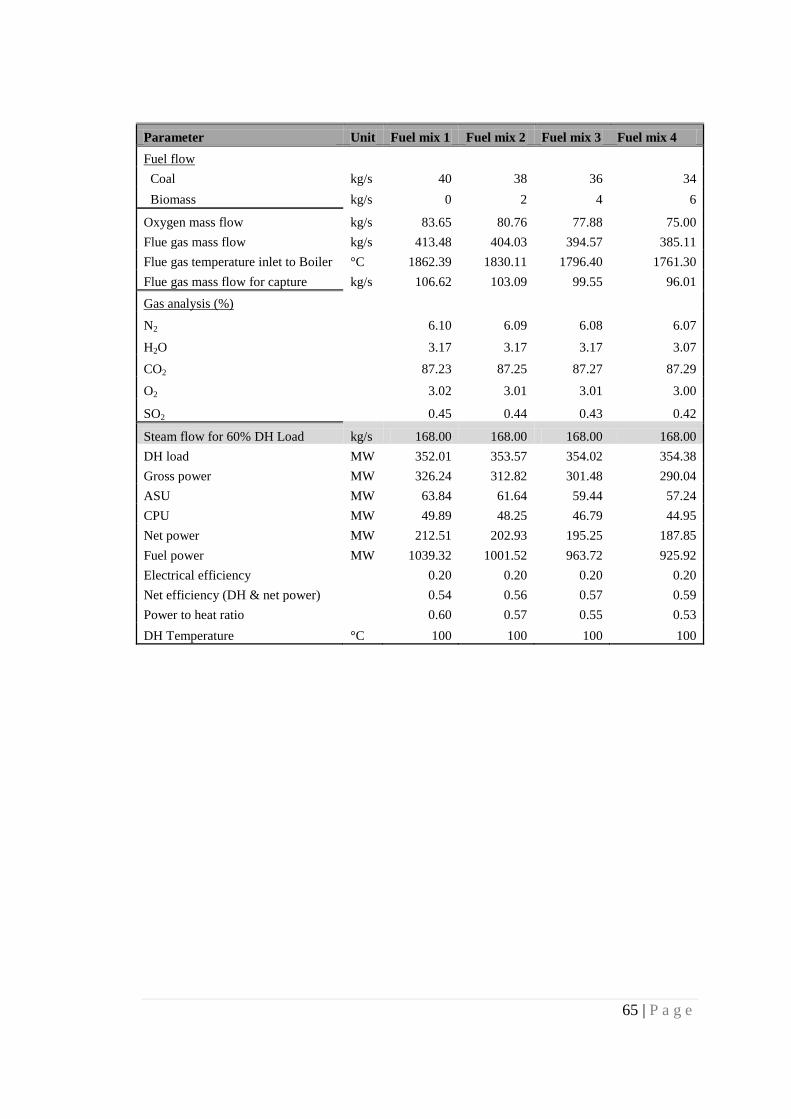
65 | P a g e
Parameter Unit Fuel mix 1 Fuel mix 2 Fuel mix 3 Fuel mix 4
Fuel flow
Coal kg/s 40 38 36 34
Biomass kg/s 0 2 4 6
Oxygen mass flow kg/s 83.65 80.76 77.88 75.00
Flue gas mass flow kg/s 413.48 404.03 394.57 385.11
Flue gas temperature inlet to Boiler °C 1862.39 1830.11 1796.40 1761.30
Flue gas mass flow for capture kg/s 106.62 103.09 99.55 96.01
Gas analysis (%)
N2
6.10 6.09 6.08 6.07
H2O
3.17 3.17 3.17 3.07
CO2
87.23 87.25 87.27 87.29
O2
3.02 3.01 3.01 3.00
SO2
0.45 0.44 0.43 0.42
Steam flow for 60% DH Load kg/s 168.00 168.00 168.00 168.00
DH load MW 352.01 353.57 354.02 354.38
Gross power MW 326.24 312.82 301.48 290.04
ASU MW 63.84 61.64 59.44 57.24
CPU MW 49.89 48.25 46.79 44.95
Net power MW 212.51 202.93 195.25 187.85
Fuel power MW 1039.32 1001.52 963.72 925.92
Electrical efficiency
0.20 0.20 0.20 0.20
Net efficiency (DH & net power)
0.54 0.56 0.57 0.59
Power to heat ratio
0.60 0.57 0.55 0.53
DH Temperature °C 100 100 100 100

66 | P a g e
Design case 3: (Fuel mix 1 & DH 70%)
Parameter Unit Fuel mix 1 Fuel mix 2 Fuel mix 3 Fuel mix 4
Fuel flow
Coal kg/s 40 38 36 34
Biomass kg/s 0 2 4 6
Oxygen mass flow kg/s 83.65 80.76 77.88 75.00
Flue gas mass flow kg/s 413.48 404.03 394.57 385.11
Flue gas temperature inlet to Boiler °C 1861.91 1829.73 1796.17 1761.35
Flue gas mass flow for capture kg/s 106.62 103.09 99.55 96.01
Gas analysis (%)
N2
6.10 6.09 6.08 6.07
H2O
3.17 3.17 3.17 3.07
CO2
87.23 87.25 87.27 87.29
O2
3.02 3.01 3.01 3.00
SO2
0.45 0.44 0.43 0.42
Steam flow for 100% DH Load kg/s 280 280 280 280
DH load MW 586.48 587.56 587.34 590.32
Gross power MW 311.64 296.96 283.71 266.73
ASU MW 63.84 61.64 59.44 57.24
CPU MW 49.89 48.25 46.79 44.95
Net power MW 197.91 187.07 177.48 164.54
Fuel power MW 1039.32 1001.52 963.72 925.92
Electrical efficiency
0.19 0.19 0.18 0.18
Net efficiency (DH & net power)
0.75 0.77 0.79 0.82
Power to heat ratio
0.34 0.32 0.30 0.28
DH Temperature °C 100 100 100 100
Parameter Unit Fuel mix 1 Fuel mix 2 Fuel mix 3 Fuel mix 4
Fuel flow
Coal kg/s 40 38 36 34
Biomass kg/s 0 2 4 6
Oxygen mass flow kg/s 83.65 80.76 77.88 75.00
Flue gas mass flow kg/s 413.48 404.03 394.57 385.11
Flue gas temperature inlet to Boiler °C 1861.83 1829.66 1796.09 1761.28
Flue gas mass flow for capture kg/s 106.62 103.09 99.55 96.01
Gas analysis (%)
N2
6.10 6.09 6.08 6.07
H2O
3.17 3.17 3.17 3.07
CO2
87.23 87.25 87.27 87.29
O2
3.02 3.01 3.01 3.00
SO2
0.45 0.44 0.43 0.42
Steam flow for 90% DH Load kg/s 252.00 252.00 252.00 252.00
DH load MW 528.44 529.43 529.23 531.96
Gross power MW 319.29 304.77 291.74 274.95
ASU MW 63.84 61.64 59.44 57.24
CPU MW 49.89 48.25 46.79 44.95
Net power MW 205.56 194.88 185.51 172.76
Fuel power MW 1039.32 1001.52 963.72 925.92
Electrical efficiency
0.20 0.19 0.19 0.19
Net efficiency (DH & net power)
0.71 0.72 0.74 0.76
Power to heat ratio
0.39 0.37 0.35 0.32
DH Temperature °C 100 100 100 100

67 | P a g e
Parameter Unit Fuel mix 1 Fuel mix 2 Fuel mix 3 Fuel mix 4
Fuel flow
Coal kg/s 40 38 36 34
Biomass kg/s 0 2 4 6
Oxygen mass flow kg/s 83.65 80.76 77.88 75.00
Flue gas mass flow kg/s 413.48 404.03 394.57 385.11
Flue gas temperature inlet to Boiler °C 1861.77 1829.58 1796.02 1761.21
Flue gas mass flow for capture kg/s 106.62 103.09 99.55 96.01
Gas analysis (%)
N2
6.10 6.09 6.08 6.07
H2O
3.17 3.17 3.17 3.07
CO2
87.23 87.25 87.27 87.29
O2
3.02 3.01 3.01 3.00
SO2
0.45 0.44 0.43 0.42
Steam flow for 80% DH Load kg/s 224.00 224.00 224.00 224.00
DH load MW 470.28 471.56 470.98 473.45
Gross power MW 326.67 312.34 299.46 282.85
ASU MW 63.84 61.64 59.44 57.24
CPU MW 49.89 48.25 46.79 44.95
Net power MW 212.94 202.45 193.23 180.66
Fuel power MW 1039.32 1001.52 963.72 925.92
Electrical efficiency
0.20 0.20 0.20 0.20
Net efficiency (DH & net electricity)
0.66 0.67 0.69 0.71
Power to heat ratio
0.45 0.43 0.41 0.38
DH Temperature °C 100 100 100 100
Parameter Unit Fuel mix 1 Fuel mix 2 Fuel mix 3 Fuel mix 4
Fuel flow
Coal kg/s 40 38 36 34
Biomass kg/s 0 2 4 6
Oxygen mass flow kg/s 83.65 80.76 77.88 75.00
Flue gas mass flow kg/s 413.48 404.03 394.57 385.11
Flue gas temperature inlet to Boiler °C 1861.70 1829.51 1795.95 1761.13
Flue gas mass flow for capture kg/s 106.62 103.09 99.55 96.01
Gas analysis (%)
N2
6.10 6.09 6.08 6.07
H2O
3.17 3.17 3.17 3.07
CO2
87.23 87.25 87.27 87.29
O2
3.02 3.01 3.01 3.00
SO2
0.45 0.44 0.43 0.42
Steam flow for 70% DH Load kg/s 196.00 196.00 196.00 196.00
DH load MW 411.98 412.75 412.62 414.79
Gross power MW 333.82 319.66 306.9 290.5
ASU MW 63.84 61.64 59.44 57.24
CPU MW 49.89 48.25 46.79 44.95
Net power MW 220.09 209.77 200.67 188.31
Fuel power MW 1039.32 1001.52 963.72 925.92
Electrical efficiency
0.21 0.21 0.21 0.20
Net efficiency (DH & net power)
0.61 0.62 0.64 0.65
Power to heat ratio
0.53 0.51 0.49 0.45
DH Temperature °C 100 100 100 100

68 | P a g e
Parameter Unit Fuel mix 1 Fuel mix 2 Fuel mix 3 Fuel mix 4
Fuel flow
Coal kg/s 40 38 36 34
Biomass kg/s 0 2 4 6
Oxygen mass flow kg/s 83.65 80.76 77.88 75.00
Flue gas mass flow kg/s 413.48 404.03 394.57 385.11
Flue gas temperature inlet to Boiler °C 1861.64 1829.45 1795.89 1761.06
Flue gas mass flow for capture kg/s 106.62 103.09 99.55 96.01
Gas analysis (%)
N2
6.10 6.09 6.08 6.07
H2O
3.17 3.17 3.17 3.07
CO2
87.23 87.25 87.27 87.29
O2
3.02 3.01 3.01 3.00
SO2
0.45 0.44 0.43 0.42
Steam flow for 60% DH Load kg/s 168.00 168.00 168.00 168.00
DH load MW 353.56 354.21 354.10 355.99
Gross Power MW 340.66 326.72 314.12 297.90
ASU MW 63.84 61.64 59.44 57.24
CPU MW 49.89 48.25 46.79 44.95
Net power MW 226.93 216.83 207.89 195.71
Fuel power MW 1039.32 1001.52 963.72 925.92
Electrical efficiency
0.22 0.22 0.22 0.21
Net efficiency (DH & net power)
0.56 0.57 0.58 0.60
Power to heat ratio
0.64 0.61 0.59 0.55
DH Temperature °C 100 100 100 100
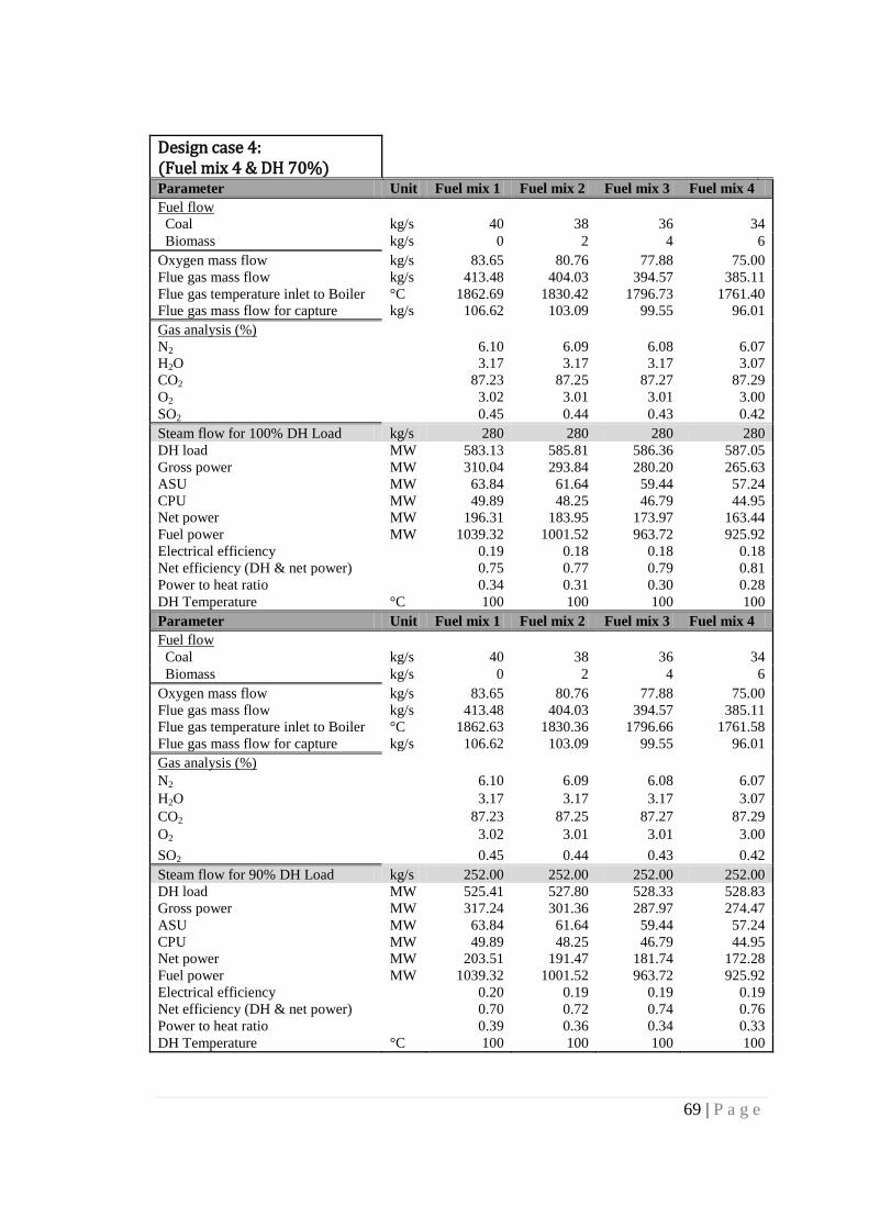
69 | P a g e
Design case 4: (Fuel mix 4 & DH 70%)
Parameter Unit Fuel mix 1 Fuel mix 2 Fuel mix 3 Fuel mix 4
Fuel flow
Coal kg/s 40 38 36 34
Biomass kg/s 0 2 4 6
Oxygen mass flow kg/s 83.65 80.76 77.88 75.00
Flue gas mass flow kg/s 413.48 404.03 394.57 385.11
Flue gas temperature inlet to Boiler °C 1862.69 1830.42 1796.73 1761.40
Flue gas mass flow for capture kg/s 106.62 103.09 99.55 96.01
Gas analysis (%)
N2
6.10 6.09 6.08 6.07
H2O
3.17 3.17 3.17 3.07
CO2
87.23 87.25 87.27 87.29
O2
3.02 3.01 3.01 3.00
SO2
0.45 0.44 0.43 0.42
Steam flow for 100% DH Load kg/s 280 280 280 280
DH load MW 583.13 585.81 586.36 587.05
Gross power MW 310.04 293.84 280.20 265.63
ASU MW 63.84 61.64 59.44 57.24
CPU MW 49.89 48.25 46.79 44.95
Net power MW 196.31 183.95 173.97 163.44
Fuel power MW 1039.32 1001.52 963.72 925.92
Electrical efficiency
0.19 0.18 0.18 0.18
Net efficiency (DH & net power)
0.75 0.77 0.79 0.81
Power to heat ratio
0.34 0.31 0.30 0.28
DH Temperature °C 100 100 100 100
Parameter Unit Fuel mix 1 Fuel mix 2 Fuel mix 3 Fuel mix 4
Fuel flow
Coal kg/s 40 38 36 34
Biomass kg/s 0 2 4 6
Oxygen mass flow kg/s 83.65 80.76 77.88 75.00
Flue gas mass flow kg/s 413.48 404.03 394.57 385.11
Flue gas temperature inlet to Boiler °C 1862.63 1830.36 1796.66 1761.58
Flue gas mass flow for capture kg/s 106.62 103.09 99.55 96.01
Gas analysis (%)
N2
6.10 6.09 6.08 6.07
H2O
3.17 3.17 3.17 3.07
CO2
87.23 87.25 87.27 87.29
O2
3.02 3.01 3.01 3.00
SO2
0.45 0.44 0.43 0.42
Steam flow for 90% DH Load kg/s 252.00 252.00 252.00 252.00
DH load MW 525.41 527.80 528.33 528.83
Gross power MW 317.24 301.36 287.97 274.47
ASU MW 63.84 61.64 59.44 57.24
CPU MW 49.89 48.25 46.79 44.95
Net power MW 203.51 191.47 181.74 172.28
Fuel power MW 1039.32 1001.52 963.72 925.92
Electrical efficiency
0.20 0.19 0.19 0.19
Net efficiency (DH & net power)
0.70 0.72 0.74 0.76
Power to heat ratio
0.39 0.36 0.34 0.33
DH Temperature °C 100 100 100 100

70 | P a g e
Parameter Unit Fuel mix 1 Fuel mix 2 Fuel mix 3 Fuel mix 4
Fuel flow
Coal kg/s 40 38 36 34
Biomass kg/s 0 2 4 6
Oxygen mass flow kg/s 83.65 80.76 77.88 75.00
Flue gas mass flow kg/s 413.48 404.03 394.57 385.11
Flue gas temperature inlet to Boiler °C 1862.57 1830.29 1796.59 1761.51
Flue gas mass flow for capture kg/s 106.62 103.09 99.55 96.01
Gas analysis (%)
N2
6.10 6.09 6.08 6.07
H2O
3.17 3.17 3.17 3.07
CO2
87.23 87.25 87.27 87.29
O2
3.02 3.01 3.01 3.00
SO2
0.45 0.44 0.43 0.42
Steam flow for 80% DH Load kg/s 224.00 224.00 224.00 224.00
DH load MW 467.56 469.66 470.16 470.61
Gross power MW 324.10 308.51 295.31 282.04
ASU MW 63.84 61.64 59.44 57.24
CPU MW 49.89 48.25 46.79 44.95
Net power MW 210.37 198.62 189.08 179.85
Fuel power MW 1039.32 1001.52 963.72 925.92
Electrical efficiency
0.20 0.20 0.20 0.19
Net efficiency (DH & net power)
0.65 0.67 0.68 0.70
Power to heat ratio
0.45 0.42 0.40 0.38
DH Temperature °C 100 100 100 100
Parameter Unit Fuel mix 1 Fuel mix 2 Fuel mix 3 Fuel mix 4
Fuel flow
Coal kg/s 40 38 36 34
Biomass kg/s 0 2 4 6
Oxygen mass flow kg/s 83.65 80.76 77.88 75.00
Flue gas mass flow kg/s 413.48 404.03 394.57 385.11
Flue gas temperature inlet to Boiler °C 1862.51 1830.23 1796.53 1761.44
Flue gas mass flow for capture kg/s 106.62 103.09 99.55 96.01
Gas analysis (%)
N2
6.10 6.09 6.08 6.07
H2O
3.17 3.17 3.17 3.07
CO2
87.23 87.25 87.27 87.29
O2
3.02 3.01 3.01 3.00
SO2
0.45 0.44 0.43 0.42
Steam flow for 70% DH Load kg/s 196.00 196.00 196.00 196.00
DH load MW 409.58 411.41 411.87 412.27
Gross power MW 330.59 315.29 302.28 289.25
ASU MW 63.84 61.64 59.44 57.24
CPU MW 49.89 48.25 46.79 44.95
Net power MW 216.86 205.40 196.05 187.06
Fuel power MW 1039.32 1001.52 963.72 925.92
Electrical efficiency
0.21 0.21 0.20 0.20
Net efficiency (DH & net power)
0.60 0.62 0.63 0.65
Power to heat ratio
0.53 0.50 0.48 0.45
DH Temperature °C 100 100 100 100

71 | P a g e
Parameter Unit Fuel mix 1 Fuel mix 2 Fuel mix 3 Fuel mix 4
Fuel flow
Coal kg/s 40 38 36 34
Biomass kg/s 0 2 4 6
Oxygen mass flow kg/s 83.65 80.76 77.88 75.00
Flue gas mass flow kg/s 413.48 404.03 394.57 385.11
Flue gas temperature inlet to Boiler °C 1862.46 1830.18 1796.47 1761.38
Flue gas mass flow for capture kg/s 106.62 103.09 99.55 96.01
Gas analysis (%)
N2
6.10 6.09 6.08 6.07
H2O
3.17 3.17 3.17 3.07
CO2
87.23 87.25 87.27 87.29
O2
3.02 3.01 3.01 3.00
SO2
0.45 0.44 0.43 0.42
Steam flow for 60% DH Load kg/s 168.00 168.00 168.00 168.00
DH load MW 351.47 353.04 353.45 353.80
Gross power MW 336.70 321.68 308.86 296.05
ASU MW 63.84 61.64 59.44 57.24
CPU MW 49.89 48.25 46.79 44.95
Net power MW 222.97 211.79 202.63 193.86
Fuel power MW 1039.32 1001.52 963.72 925.92
Electrical efficiency
0.21 0.21 0.21 0.21
Net efficiency (DH & net power)
0.55 0.56 0.58 0.59
Power to heat ratio
0.63 0.60 0.57 0.55
DH Temperature °C 100 100 100 100
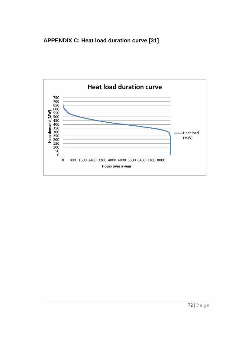
72 | P a g e
APPENDIX C: Heat load duration curve [31]
050
100150200250300350400450500550600650700750
0 800 1600 2400 3200 4000 4800 5600 6400 7200 8000
He
at d
em
and
(M
W)
Hours over a year
Heat load duration curve
Heat load(MW)

73 | P a g e
APPENDIX D: Elspot price for 2011 in Finland [35]