Embed Size (px)
Citation preview

Molecular Design and Quantum Chemistry
edited by Béla Viskolcz
Contents:
1) Introduction and overview
2) White papers
2a) Computation program (Gaussian)
2b) Vibrational analisys (written by Joseph W. Ochterski)
2c) Thermochemistry (written by Joseph W. Ochterski)
2d) NMR Computation (written by James Cheesman and Aelen Frisch)
3) Practice
3a) Input
3b) Z-matrix
4) Visualisation tools
4a) Gaussview
4b) Webtools
Appendix
Files:
INTERREG IIIA Community Initiative Program
Szegedi Tudományegyetem Prirodno-matematički fakultet, Univerzitet u Novom Sadu
„Computer-aided Modelling and Simulation in Natural Sciences“
University of Szeged,
Project No. HUSER0602/066

Molecular Design and Quantum Chemistry
1 Introduction
Most of the organic compounds have a structurally well defined carbon skeleton,
frequently denoted by R (the first letter of the word: Radical) and carry a single functional
group (G)
G-R
1.1.1—1. eq.
Simple examples of these molecular structures are:
halide organicAn Cl-R
1.1.1—2. eq.
alcohol organicAn OH-R
1.1.1—3. eq.
The purpose of classical organic chemistry is to study the structure of organic molecules
and the reaction which interconverts one organic structure to another. These interconversions
or chemical reactions need some reagents which may be inorganic or organic:
Structure1
ReagentStructure2
1.1.1—4. eq.
R - G1
ReagentR - G2
1.1.1—5. eq.
R - ClOH
-
R - OH + Cl-
1.1.1—6. eq.
When we are dealing with the structure of organic molecules we are concerned with the
architecture of the molecule and the architecture is three dimensional. The 3D-structural
chemistry is frequently referred to as stereochemistry.
Molecular structure is very important not only because it is pre-requisite knowledge for
organic synthesis but also because it predetermines the physical property, chemical reactivity
and biological activity of the organic molecule in question. In other words the architecture or
the structure of the molecules is an independent variable, while

Molecular Design and Quantum Chemistry
Physical properties
1.1.1—7. eq.
Chemical reactivities
1.1.1—8. eq.
Biological activities
1.1.1—9. eq.
are dependent variables. Consequently, we can specify symbolically such functional
dependence:
Property=f(structure)
1.1.1—10. eq.
Reactivity=F(structure)
1.1.1—11. eq.
Activity=f (structure)
1.1.1—12. eq.
Yet, we are not sure, at this time, of the explicit functional dependence. Thus, we may
only guess on the basis of accumulated experience what molecular structure will give us a
bright red color, what structural feature of a plastic may enhance chemical or biodegradability
and what drug candidate could perhaps have the desired pharmacological effect. In other
words, at this point in history, we are not in the position to do precise molecular engineering,
i.e. to design a molecular structure that delivers the desired physical, chemical and biological
characteristics. One may anticipate, at this time, that a great deal of advancement along this
line will occur in the 21st century.
1.1 Experimental Background
1.1.1 Stable structures and Transition States
The term stable structure refers to the structure of a molecule with the lowest
(minimum) internal energy (E) over a range of geometrical distortions, which the molecule
can have.

Molecular Design and Quantum Chemistry
G eom etrica l d istortion
In ternalenergy
Figure. 1.1.1—1. A schematic illustration showing that a stable structure corresponds to
a minimum of internal energy.
When comparing two different structures the energy difference (∆E) is a measure of
their relative stabilities.
G eom etrical distortion
Internal
energy
∆Ε
Figure. 1.1.1—2. A schematic illustration showing that the energy differences (∆∆∆∆E) is a
measure of relative stability.
If there is a path between the two minima, i.e. if the system can go from one minima to
another, then ∆E is related to the equilibrium constant (K) between the two stable structures
stable structure 1 stable structure 2K
1.1.1—1. eq.
If there is a path between the two structures, the geometrical distortion necessary to go
from stable structure1 to stable structure2 is called the reaction coordinate. The reaction
coordinate measures the reaction’s progress from one structure to another. In a one-step
reaction the energy rises to a maximum value, then lowers as it passes along the reaction
coordinate from the reactant state (R) to the product state (P). The energy maximum between
R and P is normally referred to as the transition state and is frequently denoted as TS or ‡. 11
The variation in energy along the reaction coordinate is frequently called the energy profile of
the chemical change from reactant to product.
1 Ruff, Csizmadia Fizikai szerves kémia

Molecular Design and Quantum Chemistry
R → [TS‡] → P
1.1.1—2. eq.
Figure 1.1.1—3. A schematic illustration showing the reaction profile for a one-step
reaction.
While ∆E is related to the equilibrium constant (K), the energy of activation (Ea), or the
barrier height, predetermines the specific rate (k), or specific velocity of the reaction
k = Ae -Ea/RT
1.1.1—3. eq
where A is the frequency factor, R is the universal gas constant and T is the absolute
temperature.
A reaction intermediate is also an energy minimum. Thus, for an overall reaction there
must be two transition states, one proceeding and one following a reaction intermediate ( I )
R → [TS‡
1] → I → [TS‡
2] → P
1.1.1—4. eq.
The corresponding reaction profile is shown in Figure 1.1.1—4
Figure 1.1.1—4. A schematic illustration showing the reaction profile for a two-step
reaction.
Reaction Coordinate
Internal energy
∆ E
Ea
R
P
Reaction Coordinate
Internal energy
∆ E
E a (1)
R
P
E a (2)
1
2

Molecular Design and Quantum Chemistry
Usually the first step, characterized by Ea(1)
, determines the overall rate of the reaction
to a good degree of approximation. The possession of this information will enable us to
consider the details, the mechanism, of the chemical reaction. Now we can expand on our
description of what the purpose of organic chemistry is. The purpose of modern organic
chemistry is to study the structure of organic molecules and their reactions as well as the
mechanisms involved in converting one organic structure to another.
In order to illustrate this, let us reconsider the reaction presented in the Introduction as
shown in 1.1.1—6. eq.:
HO-+R-Cl HO-R+Cl
-
Bond makeingBond breaking
1.1.1—5. eq.
In this reaction, we are breaking one bond and making another bond. In principle, we
have two mechanisms, but if the bond breaking and bond making are occurring
simultaneously, then we have a one-step or concerted mechanism:
HO-+R-Cl [HO--R--Cl
-]‡
HO-R+Cl-
1.1.1—6. eq.
Such a reaction is an example of a substitution (S), i.e. Cl is substituted by HO. Since
the reagent HO(-)
is negatively charged and, therefore, nucleophilic (N) or “nucleus-loving”
and because two (2) molecules (i.e. HO(-) and R-Cl) are involved in the reaction, this reaction
path is called an SN2 mechanism. In this case the reaction profile will look something like the
one shown in Figure 1.1.1—3
In contrast to the above, if the bond breaking precedes the bond making, then only one
molecule is involved; and therefore this nonsynchronous or stepwise path is called an SN1
mechanism. In this case, the bond breaking process clearly leads to a stable intermediate; thus,
the reaction profile will be like the one shown in Figure 1.1.1—4.
The two mechanisms are shown together in1.1.1—7. eq.:
HO-+R-Cl
[HO--R--Cl-]‡
HO-R+Cl-
HO-+R
++Cl
-
1.1.1—7. eq.
There are two questions associated with competing mechanisms such as the ones shown
in1.1.1—7. eq. First of all "which mechanism will dominate the reaction?" The answer to this
question is simple; the mechanism which is faster will dominate the reaction, and the one that
has the smallest overall activation energy (Ea), i.e. the lowest barrier height, will be the faster
one. The second question is "what makes one barrier lower than the other?" The answer to
this question is "the molecular structure". This was hinted at in the Introduction in equation 11
eq. Three molecular structures are given below. In Case I, the SN2 mechanism dominates. In
Case II, a mixture of SN1 and SN2 mechanisms occurs side by side and in Case III the SN1
mechanism dominates.

Molecular Design and Quantum Chemistry
H3C
H3CH3C
H3C
H3C
H3C
R= R= R=
Case I Case II Case III
Figure 1.1.1—5. A schematic illustration of how structural change (i.e. a variation in R)
can influence the dominating reaction mechanism. [See appendix 1]
1.1.2 Fundamentals of Thermodynamics and Kinetics
Both thermodynamics and kinetics are important in the elucidation of reaction
mechanisms. The area of investigation of these two topics is illustrated by the figure below.
RTGeNhRTk /#
)/( ∆−=
RTGeq eK /
0∆−
=
Kinetics
Thermodinamics
Rate=k[A]t[B]t
Keq=[C][D] / [A][B]
A+B
C+D
∆G#
∆G0
∆G0=∆H
0-T∆S
0
∆G#=∆H
#-T∆S
#
A+B C+D
A+B C+Dk
Keq
Figure1.1.2—1. A schematic illustration of the effective domain of thermodynamics and
kinetics in studying chemical reactions.

Molecular Design and Quantum Chemistry
Since not all reactions reach the equbrium we shall illustrate the thermodynamics of
reactions via the ionization of acids, which almost always reach equilibrium within a short
time.
The thermodynamics of equilibria
As may be inferred from Hiba! A hivatkozási forrás nem található., proton transfer
reactions are very fast because the energy barriers (‡1 and ‡2) along the reaction coordinates
are very small. Consequently, proton transfer equilibrium is established almost immediately.
CH3C
O
O
H
CH3C
O
O
+ H2O + H3O(+)
(-)
1.1.2—1. eq.
Keq=[CH3COO
(-)] [H3O
(+)]
[CH3COOH] [H2O]
1.1.2—2. eq.
As 1.1.2—1. eq. indicates, the equilibrium in this case is shifted to the left; thus, less
than 50% of acetic acid is dissociated in aqueous solution. The energetics of the process
certainly predetermines the position of the equilibrium and, therefore, the equilibrium
constant Keq. For this reason, a review of the basic principles of thermodynamics (usually
taught, but seldom learned in first year chemistry courses) is in order.
There are two ways to carry out an experiment, at constant pressure or at constant
volume. Most of our experiments are done in open vessels and the atmospheric pressure is
usually constant during the experiment. For a constant volume experiment, we need a sealed
piece of equipment usually referred to as an autoclave, like a pressure cooker. The two modes
of measurements, constant volume and constant pressure, yield slightly different results and
we need to give different names to these thermodynamic functions.
At constant volume, the observed heat of the reaction corresponds to the energy change
(∆E) and at constant pressure the heat of the reaction corresponds to the enthalpy change
(∆H). These two quantities do not differ from each other by very much; fundamentally the
difference is due to ∆(PV). Sometimes the difference is only RT which amounts to 0.6
kcal/mol at 300K. However, the distinction between ∆E and ∆H is important. Since most of
our experiments are carried out at constant pressure, ∆H is quoted more often than ∆E. We
might mention, in passing, that in Quantum Chemistry, ∆E needs to be augmented by a
correction term to obtain ∆H.
Thermal energy or enthalpy cannot freely be converted to work. In other words, the
conversion efficiency can never be 100%! The reason for this is due to the fact that thermal
energy and enthalpy are partially disordered and only the ordered portion can be converted to
work. The extent of disorder is proportional to the absolute temperature, T(K), and the
proportionality constant is called the entropy change: ∆S

Molecular Design and Quantum Chemistry
Extent of disorder = T∆S
1.1.2—3. eq.
This quantity, the extent of disorder, is the same for the energy and the enthalpy change.
Consequently, the portion of the energy, which is freely convertible to work, the “free energy”
or “Helmholz free energy”, corresponds to the following difference (Volume = const.):
∆A = ∆E - T∆S
1.1.2—4. eq.
One may write a similar difference for the enthalpy (Pressure = const):
∆G = ∆H - T∆S
1.1.2—5. eq.
This quantity (∆G) denotes “free enthalpy”, but it is usually referred to as “Gibbs free
energy” in honour of the great thermodynamicist Josiah W. Gibbs (1839-1903) who was
professor at Yale from 1869 until 1903.
The equilibrium constant Keq, such as the one given in 1.1.3-2 for the ionization of an
acid, is related to ∆G° according to 1.1.3-7. Note that superscript ° in ∆G° implies standard
Gibbs free energy at 1 atm pressure for gases and 1M concentration for solutions.
K eq = e -∆G°/RT
1.1.2—6. eq.
∆G° = -2.303RT log Keq
or ∆G° = -RT ln Keq
1.1.2—7. eq.
where R = 1.987 cal/mol ≈ 0.002 kcal/mol/K and T is the absolute temperature in
Kelvin units; [i.e., T(K) = 273.2 + t (°C)]. This equation clearly shows that the driving force
for any reaction is ∆G°. If ∆G°<< 0 the reaction is driven to the right (Keq >> 1); if ∆G°>> 0
then Keq << 1, and if ∆G°=0 then Keq=1.0. [For further exercise see appendix 5]

Molecular Design and Quantum Chemistry
2 White papers
����������������� �������������������������������
&� ����'���������(�� ���������'������ ���� ��(� ������� ��� �����)������������*��� ��()������ � + ��(��� ��)�� + �)����������,�'
������� ��()�'������� ���������'������ ���&�����������)���������� ��+�������� ����� �- )��������������� ����� �� �������(��� ������
(� *�����������( ��� �����- )���������)�������� ��(�'������ ��
&� �(���������' ������� �������������� ��+���' ������������*������������� �,�'��)� ��(��������� ������ ���)�' ��� ���.�� �����
�� ���' ��������)����)����������/������*�(� 0� ��� �*����������/�'���)�����������1���� ������������������ ��(� ���+���' �(��
���� �- ��� ������2� ��� �������������(��� ��� ��(���- )��������0� ������(���� ����3�
4(����� �����- )���������� ��(� �*������������ ��������� �����- )��������)�' ��� (�� ��')���(������ �5�� �� ������ ��
��+ (��������*���(������ ������ ���� �5�� ���+ (��������*�������(���� ������ ���� �5�� ���+ (���������(��� 6��� *�����*�
����*������� ���������+���' ���)�(�������� 57��-*���� ����)�7���������� �����*�8�!*��4.���������.�������9��
� ��5 �������� � ��� ����������� ���*������9"� � ��� �1���� ���������)��������������� ������ �����) ���+���' �
4��� � ��*������������ ������������������������������� *����������������� �������� ��(��� ����������� ���������� ������
��� + �*��� � ��� � 6� ������
�������)�' ��� ��(� �������������������� 0� ������8::�7�������������������� ��������������� ������
����������������,�'��� 0��� ������ �� ������� ��(������������� + �*��� )��� ���+ ������������������ ����� ��������
- )�����
&� �(���� ���"���� ���!�� ����' ���� +����)���)�' ��� ������ � ��� ��������������������/������(��� ��')������� ������
��������������� �������/ ��� �� ��)�
���-�� � ��������������� �� 6��� ������

Product InformationLast update: 15 March 2005
Gaussian 03:
Expanding the limits of Computational
Chemistry
Gaussian 03 brings enhancements and performance boosts to existing
methods along with new features applying electronic structure methods to
previously inaccessible areas of investigation and types of molecules.
Gaussian 03 is the latest in the Gaussian series of electronic structure
programs. Gaussian 03 is used by chemists, chemical engineers,
biochemists, physicists and others for research in established and emerging
areas of chemical interest.
Starting from the basic laws of quantum mechanics, Gaussian predicts the
energies, molecular structures, and vibrational frequencies of molecular
systems, along with numerous molecular properties derived from these basic
computation types. It can be used to study molecules and reactions under a
wide range of conditions, including both stable species and compounds
which are difficult or impossible to observe experimentally such as
short-lived intermediates and transition structures. This article introduces
several of its new and enhanced features.
Traditionally, proteins and other large biological molecules have been out of
the reach of electronic structure methods. However, Gaussian 03's ONIOM
method overcomes these limitations. ONIOM first appeared in Gaussian 98,
and several significant innovations in Gaussian 03 make it applicable to
much larger molecules.
This computational technique models large molecules by defining two or
three layers within the structure that are treated at different levels of
accuracy. Calibration studies have demonstrated that the resulting
predictions are essentially equivalent to those that would be produced by the
high accuracy method.
The ONIOM facility in Gaussian 03 provides substantial performance gains
for geometry optimizations via a quadratic coupled algorithm and the use of
micro-iterations. In addition, the program's option to include electronic
embedding within ONIOM calculations enables both the steric and
electrostatic properties of the entire molecule to be taken into account when
modeling processes in the high accuracy layer (e.g., an enzyme's active site).
These techniques yield molecular structures and properties results that are in
very good agreement with experiment.
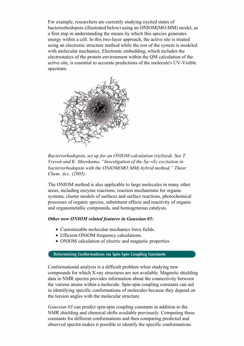
For example, researchers are currently studying excited states of
bacteriorhodopsin (illustrated below) using an ONIOM(MO:MM) model, as
a first step in understanding the means by which this species generates
energy within a cell. In this two-layer approach, the active site is treated
using an electronic structure method while the rest of the system is modeled
with molecular mechanics. Electronic embedding, which includes the
electrostatics of the protein environment within the QM calculation of the
active site, is essential to accurate predictions of the molecule's UV-Visible
spectrum.
Bacteriorhodopsin, set up for an ONIOM calculation (stylized). See T.
Vreven and K. Morokuma, “Investigation of the S0→S1 excitation in
bacteriorhodopsin with the ONIOM(MO:MM) hybrid method,” Theor.
Chem. Acc. (2003).
The ONIOM method is also applicable to large molecules in many other
areas, including enzyme reactions, reaction mechanisms for organic
systems, cluster models of surfaces and surface reactions, photochemical
processes of organic species, substituent effects and reactivity of organic
and organometallic compounds, and homogeneous catalysis.
Other new ONIOM related features in Gaussian 03:
Customizable molecular mechanics force fields.
Efficient ONIOM frequency calculations.
ONIOM calculation of electric and magnetic properties.
Conformational analysis is a difficult problem when studying new
compounds for which X-ray structures are not available. Magnetic shielding
data in NMR spectra provides information about the connectivity between
the various atoms within a molecule. Spin-spin coupling constants can aid
in identifying specific conformations of molecules because they depend on
the torsion angles with the molecular structure.
Gaussian 03 can predict spin-spin coupling constants in addition to the
NMR shielding and chemical shifts available previously. Computing these
constants for different conformations and then comparing predicted and
observed spectra makes it possible to identify the specific conformations

that were observed. In addition, the assignment of observed peaks to
specific atoms is greatly facilitated.
Gaussian 03 expands the range of chemical systems that it can model to
periodic systems such as polymers and crystals via its periodic boundary
conditions (PBC) methods. The PBC technique models these systems as
repeating unit cells in order to determine the structure and bulk properties of
the compound.
For example, Gaussian 03 can predict the equilibrium geometries and
transition structures of polymers. It can also study polymer reactivity by
predicting isomerization energies, reaction energetics, and so on, allowing
the decomposition, degradation, and combustion of materials to be studied.
Gaussian 03 can also model compounds' band gaps.
Other PBC capabilities in Gaussian 03:
2D PBC methods can be used to model surface chemistry, such as
reactions on surfaces and catalysis. In addition, using Gaussian 03
allows you to study the same problem using a surface model and/or a
cluster model, using the same basis set >and Hartree-Fock or DFT
theoretical method in both cases. Using Gaussian 03 enables you to
choose the appropriate approach for the system you are studying,
rather than being forced to frame the problem to fit the capabilities
and limitations of a particular model.
3D PBC: The structures and available bulk properties of crystals and
other three-dimensional periodic systems can be predicted.
Gaussian 03 can compute a very wide range of spectra and spectroscopic
properties. These include:
IR and Raman
Pre-resonance Raman
UV-Visible
NMR
Vibrational circular dichroism (VCD)
Electronic circular dichroism (ECD)
Optical rotary dispersion (ORD)
Harmonic vibration-rotation coupling
Anharmonic vibration and vibration-rotation coupling
g tensors and other hyperfine spectra tensors
For example, Gaussian 03 computes many of the tensors which contribute
to hyperfine spectra. These results are useful for making spectral
assignments for observed peaks, something which is usually difficult to
determine solely from the experimental data (see the example below). Using
theoretical predictions to aid in interpreting and fitting observed results
should make non-linear molecules as amenable to study as linear ones.

The observed (yellow) and computed (blue) hyperfine spectra for H2 C6 N
(N=4-3). The predicted spectrum allows spectral assignments to be made
for the observed peaks, a task which is often difficult or impossible from the
experimental data alone due to spectral overlap. Experimental data
provided by S. E. Novick, W. Chen, M. C. McCarthy and P. Thaddeus
(article in preparation).
Molecular properties and chemical reactions often vary considerably
between the gas phase and in solution. For example, low lying
conformations can have quite different energies in the gas phase and in
solution (and in different solvents), conformation equilibria can differ, and
reactions can take significantly different paths.
Gaussian 03 offers the Polarizable Continuum Model (PCM) for modeling
system in solution. This approach represents the solvent as a polarizable
continuum and places the solute in a cavity within the solvent.
The PCM facility in Gaussian 03 includes many enhancement that
significantly extend the range of problems which can be studied:
Excitation energies and related properties of excited states can be
calculated in the presence of a solvent (see the surfaces in the diagram
below).
NMR spectra and other magnetic properties.
Vibrational frequencies, IR and Raman spectra, and other properties
computed via analytic second derivatives of the energy.
Polarizabilities and hyperpolarizabilities.
General performance improvements.

(excited state-ground state)solvated - (excited state-ground state)gas phase
These surfaces represent the electron density difference between the ground
state and the charge transfer excited state in paranitroaniline (the molecule
is at the near right). The small surface at the top right shows the electron
density difference in the gas phase, and the one to its left shows the
difference in acetonitrile solution. Electron density moves from the green
areas to the red areas in the excited state.
The larger surface below the small ones is the difference of these difference
densities (solution minus gas phase), and it illustrates how the charge
transfer from NH2 to NO2 from the ground state to the excited state is
larger in solution than it is for the same gas phase transition. In addition,
as the level diagrams indicate, the ordering of the lowest two excited states
changes between the gas phase and in solution with acetonitrile (the yellow
states have 0 oscillator strengths and are not observed in ordinary
UV-Visible spectra).

Gaussian 03 Online ManualLast update: 2 October 2006
The combination of method and basis set specifies a model chemistry to Gaussian, specifying the level of theory. Every Gaussian job
must specify both a method and basis set. This is usually accomplished via two separate keywords within the route section of the input
file, although a few method keywords imply a choice of basis set.
The following table lists methods which are available in Gaussian, along with the job types for which each one may be used. Note that
the table lists only analytic optimizations, frequencies, and polarizability calculations; numerical calculations are often available for
unchecked methods (see the discussion of the specific keyword in question for details).
If no method keyword is specified, HF is assumed. Most method keywords may be prefaced by R for closed-shell restricted
wavefunctions, U for unrestricted open-shell wavefunctions, or RO for restricted open-shell wavefunctions: for example, ROHF,
UMP2, or RQCISD. RO is available only for Hartree-Fock, all Density Functional methods, AM1, MINDO3 and MNDO and PM3
semi-empirical energies and gradients, and MP2 energies; note that analytic ROMP2 gradients are not yet available.
In general, only a single method keyword should be specified , and including more than one of them will produce bizarre results.
However, there are exceptions:
CASSCF may be specified along with MP2 to request a CASSCF calculation including electron correlation.
ONIOM and IRCMax jobs require multiple method specifications. However, they are given as options to the corresponding
keyword.
The form model2 // model1 described previously may be used to generate an automatic optimization followed by a single point
calculation at the optimized geometry.
Click here to go on to the next section.

Vibrational Analysis in Gaussian
Joseph W. Ochterski, [email protected]
October 29, 1999
Abstract
One of the most commonly asked questions about Gaussian is “What is the defini-tion of reduced mass that Gaussian uses, and why is is different than what I calculatefor diatomics by hand?” The purpose of this document is to describe how Gaussian cal-culates the reduced mass, frequencies, force constants, and normal coordinates whichare printed out at the end of a frequency calculation.
Contents
1 The short answer 1
2 The long answer 22.1 Mass weight the Hessian and diagonalize . . . . . . . . . . . . . . . . . . . . 22.2 Determine the principal axes of inertia . . . . . . . . . . . . . . . . . . . . . 32.3 Generate coordinates in the rotating and translating frame . . . . . . . . . . 42.4 Transform the Hessian to internal coordinates and diagonalize . . . . . . . . 52.5 Calculate the frequencies . . . . . . . . . . . . . . . . . . . . . . . . . . . . . 52.6 Calculate reduced mass, force constants and cartesian displacements . . . . . 5
3 Summary 7
4 A note about low frequencies 8
5 Acknowledgements 10
1 The short answer
So why is the reduced mass different in Gaussian? The short answer is that Gaussian usesa coordinate system where the normalized cartesian displacement is one unit. This differsfrom the coordinate system used in most texts, where a unit step of one is used for thechange in interatomic distance (in a diatomic). The vibrational analysis of polyatomics inGaussian is not different from that described in “Molecular Vibrations” by Wilson, Decius
1

and Cross. Diatomics are simply treated the same way as polyatomics, rather than using adifferent coordinate system.
2 The long answer
In this section, I’ll describe exactly how frequencies, force constants, normal modes andreduced mass are calculated in Gaussian, starting with the Hessian, or second derivativematrix. I’ll outline the general polyatomic case, leaving out details for dealing with frozenatoms, hindered rotors and the like.
I will try to stick close to the notation used in “Molecular Vibrations” by Wilson, Deciusand Cross. I will add some subscripts to indicate which coordinate system the matrix is in.
There is an important point worth mentioning before starting. Vibrational analysis,as it’s descibed in most texts and implemented in Gaussian, is valid only when the firstderivatives of the energy with respect to displacement of the atoms are zero. In other words,the geometry used for vibrational analysis must be optimized at the same level of theoryand with the same basis set that the second derivatives were generated with. Analysis attransition states and higher order saddle points is also valid. Other geometries are notvalid. (There are certain exceptions, such as analysis along an IRC, where the non-zeroderivative can be projected out.) For example, calculating frequencies using HF/6-31g* onMP2/6-31G* geometries is not well defined.
Another point that is sometimes overlooked is that frequency calculations need to beperformed with a method suitable for describing the particular molecule being studied. Forexample, a single reference method, such as Hartree-Fock (HF) theory is not capable ofdescribing a molecule that needs a multireference method. One case that comes to mind ismolecules which are in a 2Π ground state. Using a single reference method will yield differentfrequencies for the Πx and Πy vibrations, while a multireference method shows the cylindricalsymmetry you might expect. This is seldom a large problem, since the frequencies of theother modes, like the stretching mode, are are still useful.
2.1 Mass weight the Hessian and diagonalize
We start with the Hessian matrix fCART, which holds the second partial derivatives of thepotential V with respect to displacement of the atoms in cartesian coordinates (CART):
fCARTij =
(∂2V
∂ξi∂ξj
)0
(1)
This is a 3N × 3N matrix (N is the number of atoms), where ξ1, ξ2, ξ3 · · · ξ3N are usedfor the displacements in cartesian coordinates, ∆x1,∆y1,∆z1, · · ·∆zN . The ()0 refers to thefact that the derivatives are taken at the equilibrium positions of the atoms, and that thefirst derivatives are zero.
The first thing that Gaussian does with these force constants is to convert them to mass
2

weighted cartesian coordinates (MWC).
fMWCij =fCARTij√mimj
=
(∂2V
∂qi∂qj
)0
(2)
where q1 =√m1ξ1 =
√m1∆x1, q2 =
√m1ξ2 =
√m1∆y1 and so on, are the mass weighted
cartesian coordinates.A copy of fMWC is diagonalized, yielding a set of 3N eigenvectors and 3N eigenvalues.
The eigenvectors, which are the normal modes, are discarded; they will be calculated againafter the rotation and translation modes are separated out. The roots of the eigenvalues arethe fundamental frequencies of the molecule. Gaussian converts them to cm−1, then printsout the 3N (up to 9) lowest. The output for water HF/3-21G* looks like this:
Full mass-weighted force constant matrix:Low frequencies --- -0.0008 0.0003 0.0013 40.6275 59.3808 66.4408Low frequencies --- 1799.1892 3809.4604 3943.3536
In general, the frequencies for for rotation and translation modes should be close to zero.If you have optimized to a transition state, or to a higher order saddle point, then therewill be some negative frequencies which may be listed before the “zero frequency” modes.(Freqencies which are printed out as negative are really imaginary; the minus sign is simplya flag to indicate that this is an imaginary frequency.) There is a discussion about how closeto zero is close enough, and what to do if you are not close enough in Section 4 of this paper.
You should compare the lowest real frequencies list in this part of the output with thecorresponding frequencies later in the output. The later frequencies are calculated afterprojecting out the translational and rotational modes. If the corresponding frequencies inboth places are not the same, then this is an indication that these modes are contaminatedby the rotational and translational modes.
2.2 Determine the principal axes of inertia
The next step is to translate the center of mass to the origin, and determine the momentsand products of inertia, with the goal of finding the matrix that diagonalizes the momentof inertia tensor. Using this matrix we can find the vectors corresponding to the rotationsand translations. Once these vectors are known, we know that the rest of the normal modesare vibrations, so we can distinguish low frequency vibrational modes from rotational andtranslational modes.
The center of mass (RCOM) is found in the usual way:
RCOM =
∑αmαrα∑αmα
(3)
where the sums are over the atoms, α. The origin is then shifted to the center of massrCOMα = rα−RCOM. Next we have to calculate the moments of inertia (the diagonal elements)and the products of inertia (off diagonal elements) of the moment of inertia tensor (I).
I =
Ixx Ixy IxzIyx Iyy IyzIzx Izy Izz
=
∑αmα(y2
α + z2α) −
∑αmα(xαyα) −
∑αmα(xαzα)
−∑αmα(yαxα)
∑αmα(x2
α + z2α) −
∑αmα(yαzα)
−∑αmα(zαxα) −
∑αmα(zαyα)
∑αmα(x2
α + y2α)
(4)
3

This symmetric matrix is diagonalized, yielding the principal moments (the eigenvalues I′)and a 3×3 matrix (X), which is made up of the normalized eigenvectors of I. The eigenvectorsof the moment of inertia tensor are used to generate the vectors corresponding to translationand infinitesimal rotation of the molecule in the next step.
2.3 Generate coordinates in the rotating and translating frame
The main goal in this section is to generate the transformation D from mass weighted carte-sian coordinates to a set of 3N coordinates where rotation and translation of the moleculeare separated out, leaving 3N − 6 or 3N − 5 modes for vibrational analysis. The rest ofthis section describes how the Sayvetz conditions are used to generate the translation androtation vectors.
The three vectors (D1, D2, D3) of length 3N corresponding to translation are trivial togenerate in cartesian coordinates. They are just
√mi times the corresponding coordinate
axis. For example, for water (using mH = 1 and mO = 16) the translational vectors are:
D1 = (1, 0, 0, 4, 0, 0, 1, 0, 0)t
D2 = (0, 1, 0, 0, 4, 0, 0, 1, 0)t
D3 = (0, 0, 1, 0, 0, 4, 0, 0, 1)t
Generating vectors corresponding to rotational motion of the atoms in cartesian coordi-nates is a bit more complicated. The vectors for these are defined this way:
D4j,i = ((Py)iXj,3 − (Pz)iXj,2)/√mi
D5j,i = ((Pz)iXj,1 − (Px)iXj,3)/√mi
D6j,i = ((Px)iXj,2 − (Py)iXj,1)/√mi
(5)
where j = x, y, z; i is over all atoms and P is the dot product of R (the coordinates of theatoms with respect to the center of mass) and the corresponding row of X, the matrix usedto diagonalize the moment of inertia tensor I.
The next step is to normalize these vectors. If the molecule is linear (or is a singleatoms), any vectors which do not correspond to translational or rotational normal modesare removed. The scalar product is taken of each vector with itself. If it is zero (or veryclose to it), then that vector is not an actual normal mode and it is eliminated. (If the scalarproduct is zero, this mode will disappear when the transformation from mass weighted tointernal coordinates is done, in Equation 6.) Otherwise, the vector is normalized using thereciprocal square root of the scalar product. Gaussian then checks to see that the number ofrotational and translational modes is what’s expected for the molecule, three for atoms, fivefor linear molecules and six for all others. If this is not the case, Gaussian prints an errormessage and aborts.
A Schmidt orthogonalization is used to generate Nvib = 3N − 6 (or 3N − 5) remainingvectors, which are orthogonal to the five or six rotational and translational vectors. The resultis a transformation matrix D which transforms from mass weighted cartesian coordinates qto internal coordinates S = Dq, where rotation and translation have been separated out.
4

2.4 Transform the Hessian to internal coordinates and diagonalize
Now that we have coordinates in the rotating and translating frame, we need to transform theHessian, fMWC (still in mass weighted cartesian coordinates), to these new internal coordinates(INT). Only the Nvib coordinates corresponding to internal coordinates will be diagonalized,although the full 3N coordinates are used to transform the Hessian.
The transformation is straightforward:
fINT = D†fMWCD (6)
The Nvib × Nvib submatrix of fINT, which represents the force constants internal coordi-nates, is diagonalized yielding Nvib eigenvalues λ = 4π2ν2, and Nvib eigenvectors. If we callthe transformation matrix composed of the eigenvectors L, then we have
L†fINTL = Λ (7)
where Λ is the diagonal matrix with eigenvalues λi.
2.5 Calculate the frequencies
At this point, the eigenvalues need to be converted frequencies in units of reciprocal cen-timeters. First we change from frequencies (νi) to wavenumbers (ν̃i), via the relationshipνi = ν̃ic, where c is the speed of light. Solving λ = 4π2ν̃2c2 for ν̃2
i we get
ν̃i =
√λi
4π2c2(8)
The rest is simply applying the appropriate conversion factors: from a single molecule toa mole, from hartrees to joules, and from atomic mass units to kilograms. For negativeeigenvalues, we calculate ν̃i using the absolute value of λi, then multiply by −1 to make thefrequency negative (which flags it as imaginary). After this conversion, the frequencies areready to be printed out.
2.6 Calculate reduced mass, force constants and cartesian dis-placements
All the pieces are now in place to calculate the reduced mass, force constants and cartesiandisplacements. Combining Equation 6 and Equation 7, we arrive at
L†D†fMWCDL = Λ = lMWC†fMWClMWC (9)
where l = DL is the matrix needed to diagonalize fMWC. Actually, lMWC is never calculateddirectly in Gaussian. Instead, lCART = MDL is calculated, where M is a diagonal matrixdefined by:
Mi,i = 1/√mi (10)
5

and i runs over the x, y, and z coordinates for every atom. The individual elements of lCART
are given by:
lCARTk,i =3N∑j
(Dk,jLj,i√
mj
). (11)
The column vectors of these elements, which are the normal modes in cartesian coordi-nates, are used in several ways. First of all, once normalized by the procedure describedbelow, they are the displacements in cartesian coordinates. Secondly, they are useful forcalculating a number of spectroscopic properties, including IR intensities, Raman activies,depolarizations and dipole and rotational strengths for VCD.
Normalization is a relatively straight forward process. Before it is printed out, each ofthe 3N elements of lCARTi is scaled by normalization factor Ni, for that particular vibrationalmode. The normalization is defined by:
Ni =
√√√√√( 3N∑k
lCART2k,i
)−1
(12)
The reduced mass µi for the vibrational mode is calculated in a similar fashion:
µi =
(3N∑k
lCART2k,i
)−1
=
3N∑k
(lMWCk,i√mj
)2−1
=
(3N∑k
(lMWC
2k,i
mj
))−1
= N 2i (13)
Note that since D is orthonormal, and we can (and do) choose L to be orthonormal, then l isorthonormal as well. (Since D†D = 1,L†L = 1 then l†l = (DL)†DL = L†D†DL = L†1L =1).
We now have enough information to explain the difference between the reduced massGaussian prints out, and the one calculated using the formula usually used for diatomics:
1
µ=
1
m1
+1
m2
(14)
The difference is in the numerator of each term in the summation. Gaussian uses lMWC2k,i
rather than 1. Using the elements of lMWC yields the consistent results for polyatomic cases,and automatically takes symmtery into consideration. Simply extending the formula fromEquation 14 to 1
µ=∑atomsi
1mi
would (incorrectly) yield the same reduced mass for everymode of a polyatomic molecule.
The effect of using the elements of lMWC in the numerator is to make the unit length ofthe coordinate system Gaussian uses be the normalized cartesian displacement. In otherwords, in the coordinate system that Gaussian uses, the sum of the squares of the cartesiandisplacements is 1. (You can check this in the output). In the more common coordinatesystem for diatomics, the unit length is a unit change in internuclear distance from theequilibrium value.
One of the consequences of using this coordinate system is that force constants which youthink should be equal are not. A simple example is H2 versus HD. Since the Hessian dependsonly on the electronic part of the Hamiltonian, you would expect the force constants to be
6

the same for these to molecules. In fact, the force constant Gaussian prints out is different.The different masses of the atoms leads to a different set of Sayvetz conditions, which in turn,change the internal coordinate system the force constants are transformed to, and ultimatelythe resulting force constant.
The coordinates used to calculate the force constants, the reduced mass and the carte-sian displacements are all internally consistent. The force constants ki are given by ki =
4π2ν̃2µi, since ν̃ = 12π
√kiµi
. The force constants are converted from atomic units to milli-
dyne/angstrom.
3 Summary
To summarize, the steps Gaussian uses to perform vibrational analysis are:
1. Mass weight the Hessian
fMWCij =fCARTij√mimj
2. Determine the principal axes of inertia
I′ = X†IX
3. Generate coordinates in the rotating and translating frame
S = Dq
4. Transform the Hessian to internal coordinates and diagonalize
fINT = D†fMWCD
L†fINTL = Λ
5. Calculate the frequencies
ν̃i =
√λi
4π2c2
6. Calculate reduced mass, force constants and cartesian displacements
µi =
(3N∑k
lCART2k,i
)−1
ki = 4π2ν̃2i µi
lCART = MDL
7

Criteria Low frequenciesOpt −0.0008 0.0003 0.0013 40.6275 59.3808 66.4408Opt=Tight 0.0011 0.0013 0.0015 4.1908 −6.8779 12.4224Opt=VeryTight −0.0011 0.0014 0.0015 −0.9207 −1.1831 −1.6023
Table 1: The effect of optimization criteria on the low frequencies of water using HF/3-21G*.The frequencies are sorted by increasing absolute value, so that it’s easier to distinguishrotational modes from vibrational modes.
4 A note about low frequencies
You’ll find that the frequencies for the translations are almost always extremely close tozero. The frequencies for rotations are quite a bit larger. So, how “close to zero” is closeenough? For most methods (HF, MP2, etc.), you’d like the rotational frequencies to bearound 10 wavenumbers or less. For methods which use numerical integration, like DFT,the frequencies should be less than a few tens of wavenumbers, say 50 or so.
If the frequencies for rotations are not close to zero, it may be a signal that you need todo a tighter optimization. There are a couple of ways to accomplish this. For most methods,you can use Opt=Tight or Opt=Verytight on the route card to specify that you’d like to usetighter convergence criteria. For DFT, you may also need to specify Int=Ultrafine, whichuses a more accurate numerical integration grid.
As an example, I reran the water HF/3-21G* calculation above, with both Opt=Tightand Opt=VeryTight. You can see in Table 1 that the rotational frequencies are an order ofmagnitude better for Opt=Tight than they were for just Opt. Using Opt=Verytight makesthem even better. This raises the question of whether the you need to use tighter convergence.The answer is: it depends – different users will be interested in different results. There is atrade off between accuracy and speed. Using Opt=Tight or Int=Ultrafine makes the calulationtake longer in addition to making the results more accurate. The default convergence criteriaare set to give an accuracy good enough for most purposes without spending time to convergethe results beyond this accuracy. You may find that you need to use the tighter criteria tocompare to spectroscopic values, or to resolve a strucutre witha particularly flat potentialenergy surface.
In the water frequency calculation above, using tighter convergence criteria makes almostno difference in terms of energy or bond lengths, as Table 2 demonstrates. The energy isconverged to less then 1 microHartree, and the OH bond length is converged to 0.0002angstroms. Tightening up the convergence criteria is useful for getting a couple of extradigits of precision in the symmetric stretch frequency.
You can also see that the final geometry parameters obtained with the default optimiza-tion criteria depend somewhat on the initial starting geometry. Using Opt=VeryTight allbut eliminates these differences. I’ve included the starting geometries in Table 3, for thosewho wish to reproduce these results. (Using the default convergence criteria may give some-what different results than those I’ve shown if you use a different machine, or even the samemachine using different libraries or a different version of the compiler).
With DFT, Opt=VeryTight alone is not necessarily enough to converge the geometry to
8

Start Symmetric Antisymm.Criteria Geom Energy ROH AHOH Bend Stretch Stretch
Opt A −75.5859596012 0.9669 107.7241 1799.1892 3809.4604 3943.3536Opt B −75.5859596488 0.9665 107.6348 1799.5957 3814.2216 3947.2011
Opt=Tight A −75.5859597578 0.9667 107.6784 1799.3335 3812.3499 3945.7723Opt=Tight B −75.5859597580 0.9667 107.6811 1799.3156 3812.2440 3945.6938
Opt=Verytight A −75.5859597582 0.9667 107.6818 1799.2877 3812.3779 3945.8339Opt=Verytight B −75.5859597582 0.9667 107.6820 1799.2854 3812.3847 3945.8418
Table 2: The default optimization settings yield results accurate enough for most purposes.Tighter optimizations make almost no difference for this HF/3-21G* frequency calculationon water.
Geometry A Geometry BO OH,1,R2 H,1,R2H,1,R2,2,A3 H,1,R2,2,A3
R2=0.96 R2=1.0A3=109.47122063 A3=109.5
Table 3: Initial geometries for water optimization calculations. Geometry A was producedby Geom=ModelA. Geometry B is a slightly modified version of Geometry A.
the point where the low frequencies are as close to zero as you would like. To demonstratethis, I have run B3LYP/3-21G* optimizations on water, starting with geometry B fromTable 3, with Opt, Opt=Tight and Opt=VeryTight. The results are in Table 4. The lowfrequencies from these two jobs hardly change, and in fact get worse for the Tight andVeryTight optimizations.
Given the straight forward convergence seen with Hartree-Fock theory, this might notseem to make sense. However, it does make sense if you recall that DFT is done usinga numerical integration on a grid of points. The accuracy of the default grid is not highenough for computing low frequency modes very precisely. The solution is to use a morenumerically accurate grid. The tighter the optimzation criteria, the more accurate the gridneeds to be. As you can see in Table 4, increasinfg the convergence criteria from Tightto VeryTight without increasing the numerical accuracy of the grid yields no improvementin the low frequencies. For Opt=Tight, we recommend using the Ultrafine grid. This is agood combination to use for systems with hindered rotors, or if exact conformation is ofconcern. If still more accuracy is necessary, then an unpruned 199974 grid can be used withOpt=VeryTight. Again, the higher accuracy comes at a higher cost in terms of CPU time.The VeryTight optimization with a 199974 grid is very expensive, even for medium sizedmolecules. The default grids are accurate enough for most purposes.
9

Criteria Grid Low frequenciesOpt FineGrid −0.0005 −0.0011 0.0011 16.5776 17.8265 −38.2354Opt=Tight FineGrid −0.0011 −0.0011 0.0005 25.8979 −29.0202 37.0170Opt=VeryTight FineGrid −0.0006 −0.0007 −0.0008 25.8977 −29.0203 37.0168Opt=Tight UltraFine 0.0012 0.0022 0.0024 −1.5386 −4.8182 −9.0313Opt=VeryTight UltraFine 0.0012 0.0022 0.0024 −1.5386 −4.8182 −9.0313Opt=VeryTight Grid=199974 −0.0004 0.0010 0.0011 −4.8721 −5.3561 −6.3672
Table 4: The effect of grid size on the low frequencies from B3LYP/3-21G* on water withOpt, Opt=Tight and Opt=VeryTight. More accurate grids are necessary for a truly convergedoptimization. The frequencies are sorted by increasing absolute value, so that it’s easier todistinguish rotational modes from vibrational modes.
5 Acknowledgements
I’d like to thank John Montgomery for his constructive suggestions, Michael Frisch for clari-fying several points, and H. Berny Schlegel for taking the time to discuss this material withme. Thanks also to Jim Cheeseman, for lending me his copy of Wilson, Decius and Cross.
10

Thermochemistry in Gaussian
Joseph W. Ochterski, [email protected]
c©2000, Gaussian, Inc.
June 2, 2000
Abstract
The purpose of this paper is to explain how various thermochemical values arecomputed in Gaussian. The paper documents what equations are used to calculatethe quantities, but doesn’t explain them in great detail, so a basic understandingof statistical mechanics concepts, such as partition functions, is assumed. Gaussianthermochemistry output is explained, and a couple of examples, including calculatingthe enthalpy and Gibbs free energy for a reaction, the heat of formation of a moleculeand absolute rates of reaction are worked out.
Contents
1 Introduction 2
2 Sources of components for thermodynamic quantities 22.1 Contributions from translation . . . . . . . . . . . . . . . . . . . . . . . . . . 32.2 Contributions from electronic motion . . . . . . . . . . . . . . . . . . . . . . 42.3 Contributions from rotational motion . . . . . . . . . . . . . . . . . . . . . . 42.4 Contributions from vibrational motion . . . . . . . . . . . . . . . . . . . . . 6
3 Thermochemistry output from Gaussian 83.1 Output from a frequency calculation . . . . . . . . . . . . . . . . . . . . . . 83.2 Output from compound model chemistries . . . . . . . . . . . . . . . . . . . 11
4 Worked-out Examples 114.1 Enthalpies and Free Energies of Reaction . . . . . . . . . . . . . . . . . . . . 124.2 Rates of Reaction . . . . . . . . . . . . . . . . . . . . . . . . . . . . . . . . . 124.3 Enthalpies and Free Energies of Formation . . . . . . . . . . . . . . . . . . . 14
5 Summary 17
1

1 Introduction
The equations used for computing thermochemical data in Gaussian are equivalent to thosegiven in standard texts on thermodynamics. Much of what is discussed below is coveredin detail in “Molecular Thermodynamics” by McQuarrie and Simon (1999). I’ve cross-referenced several of the equations in this paper with the same equations in the book, tomake it easier to determine what assumptions were made in deriving each equation. Thesecross-references have the form [McQuarrie, §7-6, Eq. 7.27] which refers to equation 7.27 insection 7-6.
One of the most important approximations to be aware of throughout this analysis isthat all the equations assume non-interacting particles and therefore apply only to an idealgas. This limitation will introduce some error, depending on the extent that any systembeing studied is non-ideal. Further, for the electronic contributions, it is assumed that thefirst and higher excited states are entirely inaccessible. This approximation is generally nottroublesome, but can introduce some error for systems with low lying electronic excitedstates.
The examples in this paper are typically carried out at the HF/STO-3G level of theory.The intent is to provide illustrative examples, rather than research grade results.
The first section of the paper is this introduction. The next section of the paper, I give theequations used to calculate the contributions from translational motion, electronic motion,rotational motion and vibrational motion. Then I describe a sample output in the thirdsection, to show how each section relates to the equations. The fourth section consists ofseveral worked out examples, where I calculate the heat of reaction and Gibbs free energy ofreaction for a simple bimolecular reaction, and absoloute reaction rates for another. Finally,an appendix gives a list of the all symbols used, their meanings and values for constants I’veused.
2 Sources of components for thermodynamic quanti-
ties
In each of the next four subsections of this paper, I will give the equations used to calculatethe contributions to entropy, energy, and heat capacity resulting from translational, elec-tronic, rotational and vibrational motion. The starting point in each case is the partitionfunction q(V, T ) for the corresponding component of the total partition function. In thissection, I’ll give an overview of how entropy, energy, and heat capacity are calculated fromthe partition function.
The partition function from any component can be used to determine the entropy con-tribution S from that component, using the relation [McQuarrie, §7-6, Eq. 7.27]:
S = NkB +NkB ln
(q(V, T )
N
)+NkBT
(∂ ln q
∂T
)V
The form used in Gaussian is a special case. First, molar values are given, so we candivide by n = N/NA, and substitute NAkB = R. We can also move the first term into the
2

logarithm (as e), which leaves (with N = 1):
S = R +R ln (q(V, T )) +RT
(∂ ln q
∂T
)V
= R ln (q(V, T )e) +RT
(∂ ln q
∂T
)V
= R
(ln(qtqeqrqve) + T
(∂ ln q
∂T
)V
)(1)
The internal thermal energy E can also be obtained from the partition function [Mc-Quarrie, §3-8, Eq. 3.41]:
E = NkBT2
(∂ ln q
∂T
)V
, (2)
and ultimately, the energy can be used to obtain the heat capacity [McQuarrie, §3.4,Eq. 3.25]:
CV =
(∂E
∂T
)N,V
(3)
These three equations will be used to derive the final expressions used to calculate thedifferent components of the thermodynamic quantities printed out by Gaussian.
2.1 Contributions from translation
The equation given in McQuarrie and other texts for the translational partition function is[McQuarrie, §4-1, Eq. 4.6]:
qt =
(2πmkBT
h2
)3/2
V.
The partial derivative of qt with respect to T is:(∂ ln qt
∂T
)V
=3
2T
which will be used to calculate both the internal energy Et and the third term in Equation 1.The second term in Equation 1 is a little trickier, since we don’t know V . However, for
an ideal gas, PV = NRT =(nNA
)NAkBT , and V = kBT
P. Therefore,
qt =
(2πmkBT
h2
)3/2kBT
P.
which is what is used to calculate qt in Gaussian. Note that we didn’t have to make thissubstitution to derive the third term, since the partial derivative has V held constant.
The translational partition function is used to calculate the translational entropy (whichincludes the factor of e which comes from Stirling’s approximation):
St = R(
ln(qte) + T(
3
2T
))= R(ln qt + 1 + 3/2).
3

The contribution to the internal thermal energy due to translation is:
Et = NAkBT2
(∂ ln q
∂T
)V
= RT 2(
3
2T
)=
3
2RT
Finally, the constant volume heat capacity is given by:
Ct =∂Et
∂T
=3
2R.
2.2 Contributions from electronic motion
The usual electronic partition function is [McQuarrie, §4-2, Eq. 4.8]:
qe = ω0e−ε0/kBT + ω1e
−ε1/kBT + ω2e−ε2/kBT + · · ·
where ω is the degeneracy of the energy level, εn is the energy of the n-th level.Gaussian assumes that the first electronic excitation energy is much greater than kBT .
Therefore, the first and higher excited states are assumed to be inaccessible at any tempera-ture. Further, the energy of the ground state is set to zero. These assumptions simplify theelectronic partition function to:
qe = ω0,
which is simply the electronic spin multiplicity of the molecule.The entropy due to electronic motion is:
Se = R
(ln qe + T
(∂ ln qe
∂T
)V
)= R (ln qe + 0) .
Since there are no temperature dependent terms in the partition function, the electronicheat capacity and the internal thermal energy due to electronic motion are both zero.
2.3 Contributions from rotational motion
The discussion for molecular rotation can be divided into several cases: single atoms, linearpolyatomic molecules, and general non-linear polyatomic molecules. I’ll cover each in order.
For a single atom, qr = 1. Since qr does not depend on temperature, the contributionof rotation to the internal thermal energy, its contribution to the heat capacity and itscontribution to the entropy are all identically zero.
4

For a linear molecule, the rotational partition function is [McQuarrie, §4-6, Eq. 4.38]:
qr =1
σr
(T
Θr
)where Θr = h2/8π2IkB. I is the moment of inertia. The rotational contribution to theentropy is
Sr = R
(ln qr + T
(∂ ln qr
∂T
)V
)= R(ln qr + 1).
The contribution of rotation to the internal thermal energy is
Er = RT 2
(∂ ln qr
∂T
)V
= RT 2(
1
T
)= RT
and the contribution to the heat capacity is
Cr =
(∂Er
∂T
)V
= R.
For the general case for a nonlinear polyatomic molecule, the rotational partition functionis [McQuarrie, §4-8, Eq. 4.56]:
qr =π1/2
σr
(T 3/2
(Θr,xΘr,yΘr,z)1/2)
)
Now we have(∂ ln q∂T
)V
= 32T
, so the entropy for this partition function is
Sr = R
(ln qr + T
(∂ ln qr
∂T
)V
)
= R(ln qr +3
2).
Finally, the contribution to the internal thermal energy is
Er = RT 2
(∂ ln qr
∂T
)V
= RT 2(
3
2T
)=
3
2RT
5

and the contribution to the heat capacity is
Cr =
(∂Er
∂T
)V
=3
2R.
The average contribution to the internal thermal energy from each rotational degree offreedom is RT/2, while it’s contribution to Cr is R/2.
2.4 Contributions from vibrational motion
The contributions to the partition function, entropy, internal energy and constant volumeheat capacity from vibrational motions are composed of a sum (or product) of the contri-butions from each vibrational mode, K. Only the real modes are considered; modes withimaginary frequencies (i.e. those flagged with a minus sign in the output) are ignored. Eachof the 3natoms− 6 (or 3natoms− 5 for linear molecules) modes has a characteristic vibrationaltemperature, Θv,K = hνK/kB.
There are two ways to calculate the partition function, depending on where you choosethe zero of energy to be: either the bottom of the internuclear potential energy well, orthe first vibrational level. Which you choose depends on whether or not the contributionsarising from zero-point energy will be coputed separately or not. If they are computedseparately, then you should use the bottom of the well as your reference point, otherwise thefirst vibrational energy level is the appropriate choice.
If you choose the zero reference point to be the bottom of the well (BOT), then thecontribution to the partition function from a given vibrational mode is [McQuarrie, §4-4,Eq. 4.24]:
qv,K =e−Θv,K/2T
1− e−Θv,K/T
and the overall vibrational partition function is[McQuarrie, §4-7, Eq. 4.46]:
qv =∏K
e−Θv,K/2T
1− e−Θv,K/T
On the other hand, if you choose the first vibrational energy level to be the zero of energy(V=0), then the partition function for each vibrational level is
qv,K =1
1− e−Θv,K/T
and the overall vibrational partition function is:
qv =∏K
1
1− e−Θv,K/T
Gaussian uses the bottom of the well as the zero of energy (BOT) to determine the otherthermodynamic quantities, but also prints out the V=0 partition function. Ultimately, the
6
only difference between the two references is the additional factor of Θv,K/2, (which is thezero point vibrational energy) in the equation for the internal energy Ev. In the expressionsfor heat capacity and entropy, this factor disappears since you differentiate with respect totemperature (T ).
The total entropy contribution from the vibrational partition function is:
Sv = R
(ln(qv) + T
(∂ ln q
∂T
)V
)
= R
(ln(qv) + T
(∑K
Θv,K
2T 2+∑K
(Θv,K/T2)e−Θv,K/T
1− e−Θv,K/T
))
= R
(∑K
(Θv,K
2T+ ln(1− e−Θv,K/T )
)+ T
(∑K
Θv,K
2T 2+∑K
(Θv,K/T2)e−Θv,K/T
1− e−Θv,K/T
))
= R
(∑K
ln(1− e−Θv,K/T ) +
(∑K
(Θv,K/T )e−Θv,K/T
1− e−Θv,K/T
))
= R∑K
(Θv,K/T
eΘv,K/T − 1− ln(1− e−Θv,K/T )
)
To get from the fourth line to the fifth line in the equation above, you have to multiply byeΘv,K/T
eΘv,K/T
.The contribution to internal thermal energy resulting from molecular vibration is
Ev = R∑K
Θv,K
(1
2+
1
eΘv,K/T − 1
)
Finally, the contribution to constant volume heat capacity is
Cv = R∑K
eΘv,K/T
(Θv,K/T
e−Θv,K/T − 1
)2
Low frequency modes (defined below) are included in the computations described above.Some of these modes may be internal rotations, and so may need to be treated separately,depending on the temperatures and barriers involved. In order to make it easier to correct forthese modes, their contributions are printed out separately, so that they may be subtractedout. A low frequency mode in Gaussian is defined as one for which more than five percent ofan assembly of molecules are likely to exist in excited vibrational states at room temperature.In other units, this corresponds to about 625 cm−1, 1.9×10¹³ Hz, or a vibrational temperatureof 900 K.
It is possible to use Gaussian to automatically perform some of this analysis for you, viathe Freq=HindRot keyword. This part of the code is still undergoing some improvements, soI will not go into it in detail. See P. Y. Ayala and H. B. Schlegel, J. Chem. Phys. 108 2314(1998) and references therein for more detail about the hindered rotor analysis in Gaussianand methods for correcting the partition functions due to these effects.
7

3 Thermochemistry output from Gaussian
This section describes most of the Gaussian thermochemistry output, and how it relates tothe equations I’ve given above.
3.1 Output from a frequency calculation
In this section, I intentionally used a non-optimized structure, to show more output. Forproduction runs, it is very important to use structures for which the first derivatives are zero— in other words, for minima, transition states and higher order saddle points. It is occa-sionally possible to use structures where one of the modes has non-zero first derivatives, suchas along an IRC. For more information about why it is important to be at a stationary pointon the potential energy surface, see my white paper on “Vibrational Analysis in Gaussian ”.
Much of the output is self-explanatory. I’ll only comment on some of the output whichmay not be immediately clear. Some of the output is also described in “Exploring Chemistrywith Electronic Structure Methods, Second Edition” by James B. Foresman and ÆleenFrisch.
-------------------
- Thermochemistry -
-------------------
Temperature 298.150 Kelvin. Pressure 1.00000 Atm.
Atom 1 has atomic number 6 and mass 12.00000
Atom 2 has atomic number 6 and mass 12.00000
Atom 3 has atomic number 1 and mass 1.00783
Atom 4 has atomic number 1 and mass 1.00783
Atom 5 has atomic number 1 and mass 1.00783
Atom 6 has atomic number 1 and mass 1.00783
Atom 7 has atomic number 1 and mass 1.00783
Atom 8 has atomic number 1 and mass 1.00783
Molecular mass: 30.04695 amu.
The next section gives some characteristics of the molecule based on the moments of iner-tia, including the rotational temperature and constants. The zero-point energy is calculatedusing only the non-imaginary frequencies.
Principal axes and moments of inertia in atomic units:
1 2 3
EIGENVALUES -- 23.57594 88.34097 88.34208
X 1.00000 0.00000 0.00000
Y 0.00000 1.00000 0.00001
Z 0.00000 -0.00001 1.00000
THIS MOLECULE IS AN ASYMMETRIC TOP.
ROTATIONAL SYMMETRY NUMBER 1.
ROTATIONAL TEMPERATURES (KELVIN) 3.67381 0.98044 0.98043
8
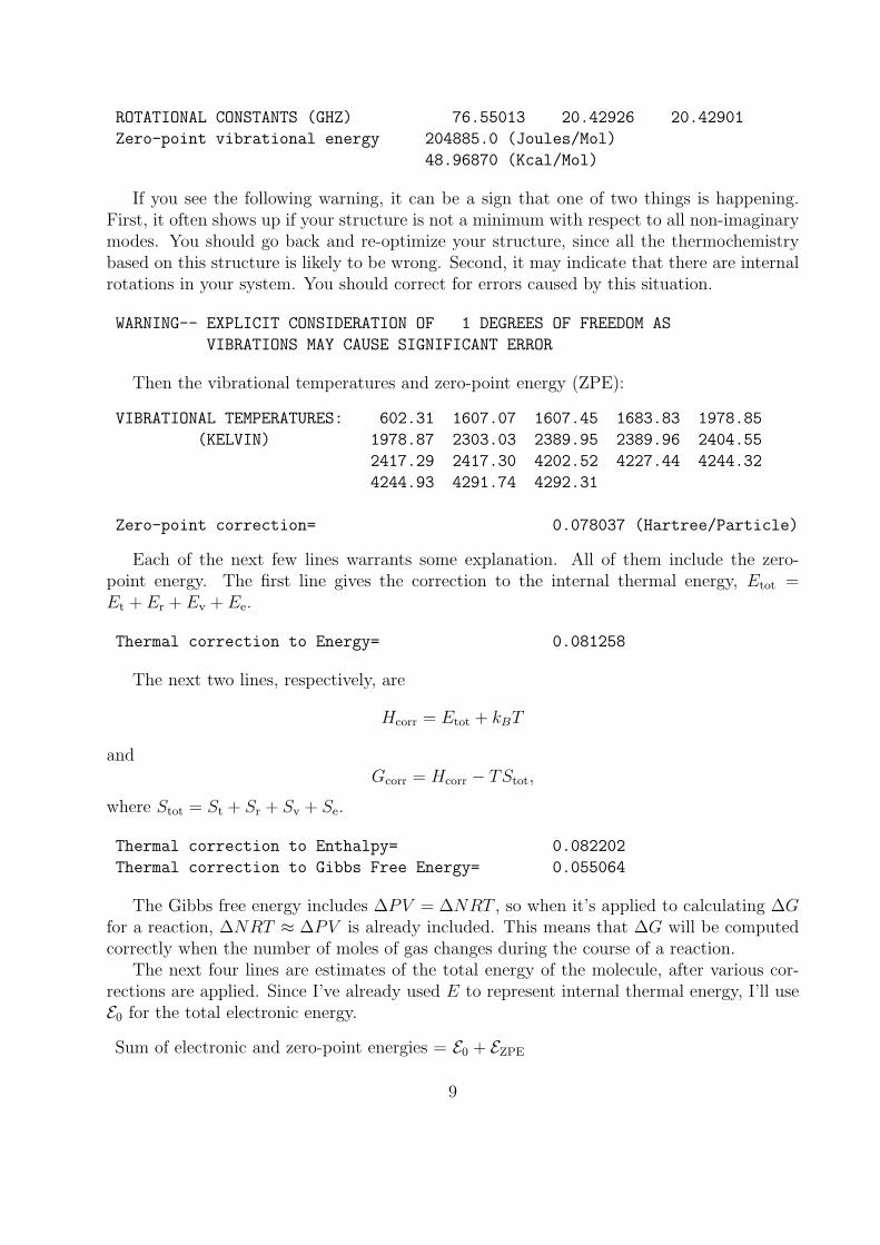
ROTATIONAL CONSTANTS (GHZ) 76.55013 20.42926 20.42901
Zero-point vibrational energy 204885.0 (Joules/Mol)
48.96870 (Kcal/Mol)
If you see the following warning, it can be a sign that one of two things is happening.First, it often shows up if your structure is not a minimum with respect to all non-imaginarymodes. You should go back and re-optimize your structure, since all the thermochemistrybased on this structure is likely to be wrong. Second, it may indicate that there are internalrotations in your system. You should correct for errors caused by this situation.
WARNING-- EXPLICIT CONSIDERATION OF 1 DEGREES OF FREEDOM AS
VIBRATIONS MAY CAUSE SIGNIFICANT ERROR
Then the vibrational temperatures and zero-point energy (ZPE):
VIBRATIONAL TEMPERATURES: 602.31 1607.07 1607.45 1683.83 1978.85
(KELVIN) 1978.87 2303.03 2389.95 2389.96 2404.55
2417.29 2417.30 4202.52 4227.44 4244.32
4244.93 4291.74 4292.31
Zero-point correction= 0.078037 (Hartree/Particle)
Each of the next few lines warrants some explanation. All of them include the zero-point energy. The first line gives the correction to the internal thermal energy, Etot =Et + Er + Ev + Ee.
Thermal correction to Energy= 0.081258
The next two lines, respectively, are
Hcorr = Etot + kBT
andGcorr = Hcorr − TStot,
where Stot = St + Sr + Sv + Se.
Thermal correction to Enthalpy= 0.082202
Thermal correction to Gibbs Free Energy= 0.055064
The Gibbs free energy includes ∆PV = ∆NRT , so when it’s applied to calculating ∆Gfor a reaction, ∆NRT ≈ ∆PV is already included. This means that ∆G will be computedcorrectly when the number of moles of gas changes during the course of a reaction.
The next four lines are estimates of the total energy of the molecule, after various cor-rections are applied. Since I’ve already used E to represent internal thermal energy, I’ll useE0 for the total electronic energy.
Sum of electronic and zero-point energies = E0 + EZPE
9

Sum of electronic and thermal energies = E0 + Etot
Sum of electronic and thermal enthalpies = E0 +Hcorr
Sum of electronic and thermal free energies = E0 +Gcorr
Sum of electronic and zero-point Energies= -79.140431
Sum of electronic and thermal Energies= -79.137210
Sum of electronic and thermal Enthalpies= -79.136266
Sum of electronic and thermal Free Energies= -79.163404
The next section is a table listing the individual contributions to the internal thermalenergy (Etot), constant volume heat capacity (Ctot) and entropy (Stot). For every low fre-quency mode, there will be a line similar to the last one in this table (labeled VIBRATION 1).That line gives the contribution of that particular mode to Etot, Ctot and Stot. This allowsyou to subtract out these values if you believe they are a source of error.
E (Thermal) CV S
KCAL/MOL CAL/MOL-KELVIN CAL/MOL-KELVIN
TOTAL 50.990 8.636 57.118
ELECTRONIC 0.000 0.000 0.000
TRANSLATIONAL 0.889 2.981 36.134
ROTATIONAL 0.889 2.981 19.848
VIBRATIONAL 49.213 2.674 1.136
VIBRATION 1 0.781 1.430 0.897
Finally, there is a table listing the individual contributions to the partition function. Thelines labeled BOT are for the vibrational partition function computed with the zero of energybeing the bottom of the well, while those labeled with (V=0) are computed with the zeroof energy being the first vibrational level. Again, special lines are printed out for the lowfrequency modes.
Q LOG10(Q) LN(Q)
TOTAL BOT 0.470577D-25 -25.327369 -58.318422
TOTAL V=0 0.368746D+11 10.566728 24.330790
VIB (BOT) 0.149700D-35 -35.824779 -82.489602
VIB (BOT) 1 0.419879D+00 -0.376876 -0.867789
VIB (V=0) 0.117305D+01 0.069318 0.159610
VIB (V=0) 1 0.115292D+01 0.061797 0.142294
ELECTRONIC 0.100000D+01 0.000000 0.000000
TRANSLATIONAL 0.647383D+07 6.811161 15.683278
ROTATIONAL 0.485567D+04 3.686249 8.487901
10

3.2 Output from compound model chemistries
This section explains what the various thermochemical quantities in the summary out of acompound model chemistry, such as CBS-QB3 or G2, means.
I’ll use a CBS-QB3 calculation on water, but the discussion is directly applicable to allthe other compound models available in Gaussian. The two lines of interest from the outputlook like:
CBS-QB3 (0 K)= -76.337451 CBS-QB3 Energy= -76.334615
CBS-QB3 Enthalpy= -76.333671 CBS-QB3 Free Energy= -76.355097
Here are the meanings of each of those quantities.
• CBS-QB3 (0 K): This is the total electronic energy as defined by the compound model,including the zero-point energy scaled by the factor defined in the model.
• CBS-QB3 Energy: This is the total electronic energy plus the internal thermal energy,which comes directly from the thermochemistry output in the frequency part of theoutput. The scaled zero-point energy is included.
• CBS-QB3 Enthalpy: This is the total electronic energy plus Hcorr, as it is describedabove with the unscaled zero-point energy removed. This sum is appropriate for cal-culating enthalpies of reaction, as described below.
• CBS-QB3 Free Energy: This is the total electronic energy plus Gcorr, as it is describedabove, again with the unscaled zero-point energy removed. This sum is appropriatefor calculating Gibbs free energies of reaction, also as described below.
4 Worked-out Examples
In this section I will show how to use these results to generate various thermochemicalinformation.
I’ve run calculations for each of the reactants and products in the reaction where ethylradical abstracts a hydrogen atom from molecular hydrogen:
C2H5 +H2 → C2H6 +H
as well as for the transition state (all at 1.0 atmospheres and 298.15K). The thermochemistryoutput from Gaussian is summarized in Table 1.
Once you have the data for all the relevant species, you can calculate the quantitiesyou are interested in. Unless otherwise specified, all enthalpies are at 298.15K. I’ll use298K ≈ 298.15K to shorten the equations.
11

C2H5 H2 C2H6 H CE0 −77.662998 −1.117506 −78.306179 −0.466582 −37.198393EZPE 0.070833 0.012487 0.089704 0.000000 0.000000Etot 0.074497 0.014847 0.093060 0.001416 0.001416Hcorr 0.075441 0.015792 0.094005 0.002360 0.002360Gcorr 0.046513 0.001079 0.068316 −0.010654 −0.014545E0 + EZPE −77.592165 −1.105019 −78.216475 −0.466582 −37.198393E0 + Etot −77.588501 −1.102658 −78.213119 −0.465166 −37.196976E0 +Hcorr −77.587557 −1.101714 −78.212174 −0.464221 −37.196032E0 +Gcorr −77.616485 −1.116427 −78.237863 −0.477236 −37.212938
Table 1: Calculated thermochemistry values from Gaussian for the reaction C2H5 + H2 →C2H6 +H. All values are in Hartrees.
4.1 Enthalpies and Free Energies of Reaction
The usual way to calculate enthalpies of reaction is to calculate heats of formation, and takethe appropriate sums and difference.
∆rH◦(298K) =
∑products
∆fH◦prod(298K)−
∑reactants
∆fH◦react(298K).
However, since Gaussian provides the sum of electronic and thermal enthalpies, there is ashort cut: namely, to simply take the difference of the sums of these values for the reactantsand the products. This works since the number of atoms of each element is the same onboth sides of the reaction, therefore all the atomic information cancels out, and you needonly the molecular data.
For example, using the information in Table 1, the enthalpy of reaction can be calculatedsimply by
∆rH◦(298K) =
∑(E0 +Hcorr)products −
∑(E0 +Hcorr)reactants
= ((−78.212174 +−0.464221)− (−77.587557 +−1.101714)) ∗ 627.5095
= 0.012876 ∗ 627.5095
= 8.08 kcal/mol
The same short cut can be used to calculate Gibbs free energies of reaction:
∆rH◦(298K) =
∑(E0 +Gcorr)products −
∑(E0 +Gcorr)reactants
= ((−78.237863 +−0.477236)− (−77.616485 +−1.116427)) ∗ 627.5095
= 0.017813 ∗ 627.5095
= 11.18 kcal/mol
4.2 Rates of Reaction
In this section I’ll show how to compute rates of reaction using the output from Gaussian. I’llbe using results derived from transition state theory in section 28-8 of “Physical Chemistry,
12

Compound E0 E0 +Gcorr
HF −98.572847 −98.579127HD −98.572847 −98.582608Cl −454.542193 −454.557870
HCl −455.136012 −455.146251DCl −455.136012 −455.149092F −97.986505 −98.001318
FHCl −553.090218 −553.109488FDCl −553.090218 −553.110424
Table 2: Total HF/STO-3G electronic energies and sum of electronic and thermal free ener-gies for atoms molecules and transition state complex of the reaction FH + Cl → F + HCland the deuterium substituted analog.
A Molecular Approach” by D. A. McQuarrie and J. D. Simon. The key equation (number28.72, in that text) for calculating reaction rates is
k(T ) =kBT
hc◦e−∆‡G◦/RT
I’ll use c◦ = 1 for the concentration. For simple reactions, the rest is simply plugging inthe numbers. First, of course, we need to get the numbers. I’ve run HF/STO-3G frequencycalculation for reaction FH + Cl → F + HCl and also for the reaction with deuteriumsubstituted for hydrogen. The results are summarized in Table 2. I put the total electronicenergies of each compound into the table as well to illustrate the point that the final geometryand electronic energy are independent of the masses of the atoms. Indeed, the cartesianforce constants themselves are independent of the masses. Only the vibrational analysis,and quantities derived from it, are mass dependent.
The first step in calculating the rates of these reactions is to compute the free energy ofactivation, ∆‡G◦ ((H) is for the hydrogen reaction, (D) is for deuterium reaction):
∆‡G◦(H) = −553.109488− (−98.579127 +−454.557870)
= 0.027509 Hartrees
= 0.027509 ∗ 627.5095 = 17.26 kcal/mol
∆‡G◦(D) = −553.110424− (−98.582608 +−454.557870)
= 0.030054 Hartrees
= 0.030054 ∗ 627.5095 = 18.86 kcal/mol
Then we can calculate the reaction rates. The values for the constants are listed in theappendix. I’ve taken c◦ = 1.
k(298, H) =kBT
hc◦e−∆‡G◦/RT
13

=1.380662× 10⁻²³(298.15)
6.626176× 10⁻³⁴(1)exp
(−17.26 ∗ 1000
1.987 ∗ 298.15
)= 6.2125× 10¹²e−29.13
= 1.38s−1
k(298, D) = 6.2125× 10¹² exp(−18.86 ∗ 1000
1.987 ∗ 298.15
)= 6.2125× 10¹²e−31.835
= 0.0928s−1
So we see that the deuterium reaction is indeed slower, as we would expect. Again, thesecalculations were carried out at the HF/STO-3G level, for illustration purposes, not for re-search grade results. More complex reactions will need more sophisticated analyses, perhapsincluding careful determination of the effects of low frequency modes on the transition state,and tunneling effects.
4.3 Enthalpies and Free Energies of Formation
Calculating enthalpies of formation is a straight-forward, albeit somewhat tedious task, whichcan be split into a couple of steps. The first step is to calculate the enthalpies of formation(∆fH
◦(0K)) of the species involved in the reaction. The second step is to calculate theenthalpies of formation of the species at 298K.
Calculating the Gibbs free energy of reaction is similar, except we have to add in theentropy term:
∆fG◦(298) = ∆fH
◦(298K)− T (S◦(M, 298K)−∑
S◦(X, 298K))
To calculate these quantities, we need a few component pieces first. In the descriptionsbelow, I will use M to stand for the molecule, and X to represent each element which makesup M , and x will be the number of atoms of X in M .
• Atomization energy of the molecule,∑D0(M):
These are readily calculated from the total energies of the molecule (E0(M)), the zero-point energy of the molecule (EZPE(M)) and the constituent atoms:∑
D0(M) =∑
atoms
xE0(X)− E0(M)− EZPE(M)
• Heats of formation of the atoms at 0K, ∆fH◦(X, 0K):
I have tabulated recommended values for the heats of formation of the first and secondrow atomic elements at 0K in Table 3. There are (at least) two schools of thought withrespect to the which atomic heat of formation data is most appropriate. Some authorsprefer to use purely experimental data for the heats of formation (Curtiss, et. al., J.
14

Chem. Phys. 106, 1063 (1997)). Others (Ochterski, et. al., J. Am. Chem. Soc. 117,11299 (1995)), prefer to use a combination of experiment and computation to obtainmore accurate values. The elements of concern are boron, beryllium and silicon. Ihave arranged Table 3 so that either may be used; the experimental results are on thetop, while the computational results for the three elements with large experimentaluncertainty are listed below that.
• Enthalpy corrections of the atomic elements, H◦X(298K)−H◦X(0K) :
The enthalpy corrections of the first and second row atomic elements are also includedin Table 3. These are used to convert the atomic heats of formation at 0K to thoseat 298.15K, and are given for the elements in their standard states. Since they do notdepend on the accuracy of the heat of formation of the atom, they are the same forboth the calculated and experimental data.
This is generally not the same as the output from Gaussian for a calculation onan isolated gas-phase atom. These values are referenced to the standard states ofthe elements. For example, the value for hydrogen atom is 1.01 kcal/mol. This is(H◦H2
(298K) − H◦H2(0K))/2, and not H◦H(298K) − H◦H(0K), which is what Gaussian
calculates.
• Enthalpy correction for the molecule, H◦M(298K)−H◦M(0K) :
For a molecule, this is Hcorr − EZPE(M), where Hcorr is the value printed out in theline labeled “Thermal correction to Enthalpy” in Gaussian output. Remember,though, that the output is in Hartrees/particle, and needs to be converted to kcal/mol.The conversion factor is 1 Hartree = 627.5095 kcal/mol.
• Entropy for the atoms, S◦X(298K) :
These are summarized in Table 3. The values were taken from the JANAF tables(M. W. Chase, Jr., C. A. Davies, J. R. Downey, Jr., D. J. Frurip, R. A. McDonald,and A. N. Syverud, J. Phys. Ref. Data 14 Suppl. No. 1 (1985)). Again, these valuesare referenced to the standard states of the elements, and will disagree with valuesGaussian calculates for the gas-phase isolated atoms.
• Entropy for the molecule, S◦M(298K) :
Gaussian calculates G = H − TS, and prints it out on the line labeled “Thermalcorrection to Gibbs Free Energy”. The entropy can be teased out of this usingS = (H −G)/T .
Putting all these pieces together, we can finally take the steps necessary to calculate∆fH
◦(298K) and ∆fG◦(298K):
1. Calculate ∆fH◦(M, 0K) for each molecule:
∆fH◦(M, 0K) =
∑atoms
x∆fH◦(X, 0K)−
∑D0(M)
=∑
atoms
x∆fH◦(X, 0K)−
( ∑atoms
xE0(X)− E0(M)
)
15

Experimentala
Element ∆fH◦(0K) H◦(298K)−H◦(0K) S◦(298K)
H 51.63±0.001 1.01 27.418±0.004Li 37.69±0.2 1.10 33.169±0.006Be 76.48±1.2 0.46 32.570±0.005B 136.2 ±0.2 0.29 36.672±0.008C 169.98±0.1 0.25 37.787±0.21N 112.53±0.02 1.04 36.640±0.01O 58.99±0.02 1.04 38.494±0.005F 18.47±0.07 1.05 37.942±0.001
Na 25.69±0.17 1.54 36.727±0.006Mg 34.87±0.2 1.19 8.237±d
Al 78.23±1.0 1.08 39.329±0.01Si 106.6 ±1.9 0.76 40.148±0.008P 75.42±0.2 1.28 39.005±0.01S 65.66±0.06 1.05 40.112±0.008Cl 28.59±0.001 1.10 39.481±0.001
Calculatedb
Element ∆fH◦(0K) H◦(298K)−H◦(0K) S◦(298K)
Be 75.8 ±0.8 0.46 32.570±0.005B 136.2 ±0.2 0.29 36.672±0.008Si 108.1 ±0.5 0.76 40.148±0.008
Table 3: Experimental and calculated enthalpies of formation of elements (kcal mol−1) andentropies of atoms (cal mol−1 K−1) . a Experimental enthalpy values taken from J. Chem.Phys. 106, 1063 (1997). b Calculated enthalpy values taken from J. Am. Chem. Soc. 117,11299 (1995). H◦(298K) −H◦(0K) is the same for both calculated and experimental, andis taken for elements in their standard states. c Entropy values taken from JANAF Ther-mochemical Tables: M. W. Chase, Jr., C. A. Davies, J. R. Downey, Jr., D. J. Frurip,R. A. McDonald, and A. N. Syverud, J. Phys. Ref. Data 14 Suppl. No. 1 (1985). d No errorbars are given for Mg in JANAF.
2. Calculate ∆fH◦(M, 298K) for each molecule:
∆fH◦(M, 298K) = ∆fH
◦(M, 0K) + (H◦M(298K)−H◦M(0K))
−∑
atoms
x(H◦X(298K)−H◦X(0K))
3. Calculate ∆fG◦(M, 298K) for each molecule:
∆fG◦(M, 298K) = ∆rH
◦(298K)− 298.15(S◦(M, 298K)−∑
S◦(X, 298K))
Here is a worked out example, where I’ve calculated ∆fH◦(298K) for the reactants and
products in the reaction I described above.
16

First, I’ll calculate ∆fH◦(0K) for one of the species:
∆fH◦(C2H6, 0K) = 2 ∗ 169.98 + 6 ∗ 51.63
−627.5095 ∗ (2 ∗ (−37.198393) + 6 ∗ (−0.466582)− (−78.216475))
= 649.74− 627.5095 ∗ 1.020197
= 9.56
The next step is to calculate the ∆fH◦(298K):
∆fH◦(C2H6, 298K) = 9.56 + 627.5095 ∗ (0.094005− 0.089704)− (2 ∗ 0.25 + 6 ∗ 1.01)
= 9.56 + 2.70− 6.56
= 5.70
To calculate the Gibbs free energy of formation, we have (the factors of 1000 are toconvert kcal to or from cal) :
∆fG◦(C2H6, 298K) = 5.70 + 298.15(627.5095 ∗ (0.094005− 0.068316)/298.15−
(2 ∗ 37.787 + 6 ∗ 27.418)/1000
= 5.70 + 298.15 ∗ (0.054067− 0.240082)
= −49.76
5 Summary
The essential message is this: the basic equations used to calculate thermochemical quantitiesin Gaussian are based on those used in standard texts. Since the vibrational partitionfunction depends on the frequencies, you must use a structure that is either a minimum ora saddle point. For electronic contributions to the partition function, it is assumed that thefirst and all higher states are inaccessible at the temperature the calculation is done at. Thedata generated by Gaussian can be used to calculate heats and free energies of reactions aswell as absolute rate information.
17

Appendix
Symbols
Ce = contribution to the heat capacity due to electronic motion
Cr = contribution to the heat capacity due to rotational motion
Ctot = total heat capacity (Ct + Cr + Cv + Ce)
Ct = contribution to the heat capacity due to translation
Cv = contribution to the heat capacity due to vibrational motion
Ee = internal energy due to electronic motion
Er = internal energy due to rotational motion
Etot = total internal energy (Et + Er + Ev + Ee)
Et = internal energy due to translation
Ev = internal energy due to vibrational motion
Gcorr = correction to the Gibbs free energy due to internal energy
Hcorr = correction to the enthalpy due to internal energy
I = moment of inertia
K = index of vibrational modes
N = number of moles
NA = Avogadro’s number
P = pressure (default is 1 atmosphere)
R = gas constant = 8.31441 J/(mol K) = 1.987 kcal/(mol K)
Se = entropy due to electronic motion
Sr = entropy due to rotational motion
Stot = total entropy (St + Sr + Sv + Se)
St = entropy due to translation
Sv = entropy due to vibrational motion
T = temperature (default is 298.15)
V = volume
Θr,Θr,(xyz) = characteristic temperature for rotation (in the x, y or z plane)
Θv,K = characteristic temperature for vibration K
kB = Boltzmann constant = 1.380662× 10⁻²³ J/K
εn = the energy of the n-th energy level
ωn = the degeneracy of the n-th energy level
18

σr = symmetry number for rotation
h = Planck’s constant = 6.626176× 10⁻³⁴ J s
m = mass of the molecule
n = number of particles (always 1)
qe = electronic partition function
qr = rotational partition function
qt = translational partition function
qv = vibrational partition function
EZPE = zero-point energy of the molecule
E0 = the total electronic energy, the MP2 energy for example
H◦, S◦, G◦ = standard enthalpy, entropy and Gibbs free energy — each compound is in itsstandard state at the given temperature
∆‡G◦ = Gibbs free energy of activation
c◦ = concentration (taken to be 1)
k(T ) = reaction rate at temperature T
19

1
Predicting Magnetic Properties with ChemDraw and Gaussian
By James R. Cheeseman and Æleen Frisch
Introduction
NMR chemical shifts are an important tool in characterizing molecular systems and structures. Accordingly, predicting NMR spectra is an essential feature of computational chemistry software. In this article, we’ll look at two very different NMR facilities, each of which is very useful when applied to the appropriate sort of molecules.
ChemDraw Ultra includes the CS ChemNMR Pro facility which can be used to estimate the 13C and 1H (proton) chemical shifts with respect to TMS. This facility is accessed from the Estimate menu within the product. When a molecule has been selected, the two items on the menu become active, and selecting one of them causes the NMR chemical shifts for the corresponding atom type to be calculated.
Figure 1 illustrates the use of this facility; here we estimate the 13C chemical shifts with respect to TMS for adenine. The Estimate menu and selected molecule appear on the left in the figure, and the resulting graphic output appears on the right. The latter consists of another copy of the molecule to which numbers denoting the chemical shift (in ppm) have been added at each atom location. Note that numbers are ordinary ChemDraw text labels and thus may be moved as needed in order to make them fully legible. Additional output is presented in text form via a Notepad document (which is opened automatically by ChemDraw).
Figure 1. Example CS ChemNMR Pro Output

Predicting Magnetic Properties with ChemDraw and Gaussian
2
CS ChemNMR Pro uses a heuristically-driven procedure in order to estimate chemical shifts; it starts with a base value determined from the molecular mechanics atom type of the atom in question, and then applies corrections for each of the groups to which it is bonded in order to compute its final value. This process is illustrated in this excerpt from the textual output from a calculation on taxol:
Protocol of the 13C NMR Estimation Node Estim. Base Incr. Comment (ppm rel. to TMS) C 138.5 123.3 1-ethylene -8.9 1 -C-C-C-C -7.4 1 -C 17.3 1 -C-C-C-C 14.2 1 -C-O
The main advantage of this approach to computing chemical shifts is its speed: chemical shifts can be computed almost instantaneously even for very large molecules. However, the method has an important weakness which must be kept in mind. Since it relies on a fixed set of parameters corresponding to atom types and subgroups, the method will be reliable only for molecules for which parameters are available and for which the assumptions about molecular structure and bonding which are built-in to the parameters are valid.
In simple terms, this NMR estimation method is appropriate only for ordinary organic molecules. It produces reasonable results for such systems, but becomes quite unreliable for systems with any unusual features: unusual bonding, strained systems, systems for which electron correlation is important for accurate modeling of the molecular structure or properties, and so on. In these cases, a more accurate computational method is required.
Systematic Prediction of Magnetic Properties
Gaussian 98 includes a facility for predicting magnetic properties, including NMR shielding tensors and chemical shifts. These calculations compute magnetic properties from first principles, as the mixed second derivative of the energy with respect to an applied magnetic field and the nuclear magnetic moment. As a result, they can produce high accuracy results for the entire range of molecular systems studied experimentally via NMR techniques.
Thus, Gaussian 98’s facility has several important advantages over the simple computation procedure used by CS ChemNMR Pro:
• Accurate prediction of magnetic properties for all types of molecular systems • Ability to predict chemical shifts for atoms other than hydrogen and carbon (nitrogen, phosphorous,
boron, and so on). • NMR properties can be computed as part of a systematic and self-consistent study of the molecule.

Predicting Magnetic Properties with ChemDraw and Gaussian
3
Some Sample Results
As we’ve noted, CS ChemNMR Pro does an adequate job of estimating chemical shifts for ordinary organic compounds. Taxol provides an example of this. For this molecule, CS ChemNMR Pro’s mean absolute error with respect to the observed 13C chemical shifts is 3.8 ppm, with a standard deviation of 4.6, and the largest error is 19.0 ppm. Gaussian also does well for this molecule: its mean absolute error is 4.2, with a standard deviation of 3.8 and a maximum error of 23.6.

Predicting Magnetic Properties with ChemDraw and Gaussian
4
Table 1 presents 13C chemical shifts for adenine as computed by CS ChemNMR Pro and predicted by Gaussian 98, comparing them to the experimentally observed values. For this molecule, Gaussian 98 performs slightly better than CS ChemNMR Pro. However, the errors that Gaussian makes are systematic, always over estimating the magnitude of the chemical shift. In contrast, the estimated shifts computed by CS ChemNMR Pro contain large errors with respect to the observed values in both directions.
Table 1. Predicted 13C Chemical Shifts for Adenine
Atom CS ChemNMR Pro ∆Experiment Gaussian 98 ∆Experiment Experiment C1 150.2 -2.2 161.2 +9.2 152.4 C2 154.9 +3.6 156.8 +5.5 151.3 C3 147.9 +8.6 139.5 +0.2 139.3 C4 128.4 +10.8 124.8 +7.2 117.6 C5 144.8 -10.5 160.7 +5.4 155.3
Table 2 lists the estimated and predicted 13C chemical shifts for a series of three strained system, cyclopropane, bicyclobutane and [1.1.1]propellane, and for another unusual system, oxaspiropentene (left to right in the illustration). Both values for the carbon shift in cyclopropane are reasonable, but with the larger molecules, the limitations of the heuristically-based approach become clear. CS ChemNMR Pro cannot estimate either the values of the chemical shifts nor the difference in shift between the two different types of carbon atoms within the molecule. Finally, the results for oxaspiropentene are only fair. In contrast, the values predicted by Gaussian 98agree very well with with the observed values in all cases.
Table 2. Chemical Shifts for Three Strained Hydrocarbons
Molecule and Atom CS ChemNMR Pro Gaussian 98 Experiment
Cyclopane (C3H6)
C1 -2.8 -6.7 -4.0
Bicyclobutane ( C5H6)
C1 6.6 26.6 32.0
C2 -0.2 -7.1 -5.7
Shift Difference 6.8 33.7 37.7

Predicting Magnetic Properties with ChemDraw and Gaussian
5
Molecule and Atom CS ChemNMR Pro Gaussian 98 Experiment
[1.1.1]Propellane(C5H6)
C1 30.3 70.6 79.3
C2 26.0 -3.4 3.4
Shift Difference 4.3 74.0 82.7
Oxaspiropentene
C1 46.0 39.2 38.9
C2 129.3 120.8 116.7
C3 44.6 31.13 30.76
Table 3 lists some sample results for predicted 15N and 11B chemical shifts as predicted by Gaussian 98. The predicted values are again in very good agreement with experimental observations.
Table 3. Predicted 15N and 11B Chemical Shifts
Molecule and Atom Gaussian 98 Experiment
C2B3H5
C 99.9 103.3
Bb -0.1 3.5
CH3CN
C -4.1 0.4
C 114.3 114.3
Nc 290.8 272.6
bShift with respect to B2H6. cShift with respect to NH3.
Selected References
All reported Gaussian 98 chemical shifts except those for taxol were computed via NMR calculations using the B3LYP/6-311+G(2d,p) level at the B3LYP/6-31G(d) optimized geometries. The taxol chemical shifts were computed from NMR calculations performed at the HF/6-31G(d) level using STO-3G optimized geometries.
“A comparison of models for calculating nuclear magnetic resonance shielding tensors,” James R. Cheeseman, Gary W. Trucks, Todd A. Keith and Michael J. Frisch, J. Chem. Phys. 104 (1996) 5497. [A discussion of the method used to predict magnetic properties as well as results for a wide variety of molecules. See the references to this paper for the sources of the experimental values cited here.]
“Synthesis of Oxaspiropentene,” W. E. Billups, Vladislav A. Litosh, Rajesh K. Saini and Andrew D. Daniels, Org. Lett. 1 (1999) 115. [NMR predictions are used to confirm the identiy of the synthesized compound.]

Predicting Magnetic Properties with ChemDraw and Gaussian
6
“NMR Chemical Shifts. 3. A Comparison of Acetylene, Allene, and the Higher Cumulenes,” Kenneth B. Wiberg, Jack D. Hammer, Kurt W. Zilm and James R. Cheeseman, J. Org. Chem. 64 (1999) 6394. [An example of a recent application study using the Gaussian NMR facility.]
“NMR Methods Blossom,” Chemical and Engineering News, 76:39, 28 September 1999. [Overview of a recent ACS symposium on NMR.]
Acknowledgments The authors thank Ken Wiberg, Berny Schlegel, Andrew Daniels, Gustavo Scuseria and Mike Frisch for their invaluable assistance in preparing this article.

Molecular Design and Quantum Chemistry
3 Practice
Gaussian 03 Online ManualLast update: 2 October 2006
Gaussian 03 input consists of a series of lines in an ASCII text file. The basic structure of
a Gaussian input file includes several different sections:
Link 0 Commands: Locate and name scratch files (not blank line terminated).
Route section (# lines): Specify desired calculation type, model chemistry and other
options (blank line terminated).
Title section: Brief description of the calculation (blank line terminated).
Molecule specification: Specify molecular system to be studied (blank line
terminated).
Optional additional sections: Additional input needed for specific job types (usually
blank line terminated).
Many Gaussian 03 jobs will include only the second, third, and fourth sections. Here is an
example of such a file, which requests a single point energy calculation on water:
# HF/6-31G(d) Route section
water energy Title section
0 1 Molecule specification O -0.464 0.177 0.0 H -0.464 1.137 0.0
H 0.441 -0.143 0.0
In this job, the route and title sections each consist of a single line. The molecule
specification section begins with a line giving the charge and spin multiplicity for the
molecule: 0 charge (neutral molecule) and spin multiplicity 1 (singlet) in this case. The
charge and spin multiplicity line is followed by lines describing the location of each atom
in the molecule; this example uses Cartesian coordinates to do so. Molecule specifications
are discussed in more detail later in this chapter.

The following input file illustrates the use of Link 0 commands and an additional input
section:
%Chk=heavy Link 0 section
#HF/6-31G(d) Opt=ModRedundant Route section
Opt job Title section
0 1 Molecule Specification section
atomic coordinates …
3 8 Add a bond and an angle to the internal
2 1 3 coordinates used during the geom. opt.
This job requests a geometry optimization. The input section following the molecule
specification is used by the Opt=ModRedundant keyword, and it serves to add an
additional bond and angle in the internal coordinates used in the geometry optimization.
The job also specifies a name for the checkpoint file.
Link 0 commands were introduced in the last chapter and are discussed individually in the
penultimate section of this chapter. The remaining input sections are discussed in the
subsequent subsections of this introductory section. For convenience, the table below lists
all possible sections that might appear within a Gaussian 03 input file, along with the
keywords associated with each one.

In general, Gaussian input is subject to the following syntax rules:
Input is free-format and case-insensitive.
Spaces, tabs, commas, or forward slashes can be used in any combination to
separate items within a line. Multiple spaces are treated as a single delimiter.
Options to keywords may be specified in any of the following forms:
keyword = option
keyword(option)
keyword=(option1, option2, ...)
keyword(option1, option2, ...)
Multiple options are enclosed in parentheses and separated by any valid delimiter
(commas are conventional and are shown above). The equals sign before the
opening parenthesis may be omitted, or spaces may optionally be included before
and/or after it.
Note that some options also take values; in this case, the option name is followed by
an equals sign: for example, CBSExtrap(NMin=6).
All keywords and options may be shortened to their shortest unique abbreviation
within the entire Gaussian 03 system. Thus, the Conventional option to the SCF
keyword may be abbreviated to Conven, but not to Conv (due to the presence of the
Convergence option). This holds true whether or not both Conventional and
Convergence happen to be valid options for any given keyword.
The contents of an external file may be included within a Gaussian 03 input file
using the following syntax: @filename. This causes the entire file to be placed at the
current location in the input stream. Appending /N to such commands will prevent
the included file's contents from being echoed at the start of the output file.
Comments begin with an exclamation point (!), which may appear anywhere on a
line. Separate comment lines may appear anywhere within the input file.
Gaussian 03 Input Section Ordering
Section KeywordsFinal blank
line?
Link 0 commands % commands no
Route Section (# lines) all yes
Extra Overlays ExtraOverlays yes
Title section all yes
Molecule specification all yes
Connectivity specifications Geom=Connect or ModConnect yes
Modifications to coordinates Opt=ModRedundant yes
2nd title and molecule
specificationOpt=QST2 or QST3 yes
Connectivity specifications for
2nd
set of coordinates
Geom=Connect or ModConnect
and
Opt=ModRedun and QST2 or
QST3
yes
Modifications to 2nd set of
coordinates
Opt=ModRedun and QST2 or
QST3yes
3rd title and initial TS structure Opt=QST3 yes for both

Connectivity specifications for
3rd
set of coordinates
Geom=Connect or ModConnect
Opt=(ModRedun, QST3)yes
Modifications to 3rd set of
coordinatesOpt=(ModRedun, QST3) yes
Atomic masses IRC=ReadIsotopes yes
Frequency of interest CPHF=RdFreq yes
Molecular Mechanics parameters HardFirst, SoftFirst, SoftOnly,
Modify yes
Initial force constants (Cartesian) Opt=FCCards yes
Accuracy of energy & forces Opt=ReadError no
BOMD/ADMP input (1 or more
sections)ADMP and BOMD yes
Basis set specification Gen, GenECP, ExtraBasis yes
Basis set alterations Massage yes
Finite field coefficients Field=Read yes
ECP specificationExtraBasis, Pseudo=Cards,
GenECPyes
Density fitting basis set
specificationExtra Density Basis yes
Background charge distribution Charge yes
Symmetry types to combine Guess=LowSymm no
Orbital specifications (separate α
& β)Guess=Cards yes
Orbital alterations (separate α &
β)Guess=Alter yes
Orbital reordering (separate α &
β)Guess=Permute yes
PCM solvation model input SCRF=Read yes
Weights for CAS state averaging CASSCF=StateAverage no
States of interest for spin orbit
couplingCASSCF=Spin no
# Orbitals/GVB pair GVB no
Atoms list for spin-spin coupling
constants NMR=ReadAtoms yes
Alternate atomic radii Pop=ReadRadii or ReadAtRadii yes
Data for electrostatic properties Prop=Read or Opt yes
Cube filename (& Cards input) Cube yes
NBO input Pop=NBORead no
Orbital freezing information ReadWindow options yes
OVGF orbitals to refine OVGF=ReadOrbitals yes
Temperature, pressure, atomic
massesFreq=ReadIsotopes no
PROAIMS/Pickett output
filenameOutput=WFN or Pickett no
Click here to go on to the next section.

Gaussian 03 Online ManualLast update: 2 October 2006
This page presents a brief overview of traditional Z-matrix descriptions of
molecular systems.
Using Internal Coordinates
Each line of a Z-matrix gives the internal coordinates for one of the atoms
within the molecule. The most-used Z-matrix format uses the following
syntax:
Element-label, atom 1, bond-length, atom 2, bond-angle, atom 3,
dihedral-angle [,format-code]
Although these examples use commas to separate items within a line, any
valid separator may be used. Element-label is a character string consisting
of either the chemical symbol for the atom or its atomic number. If the
elemental symbol is used, it may be optionally followed by other
alphanumeric characters to create an identifying label for that atom. A
common practice is to follow the element name with a secondary
identifying integer: C1, C2, etc.
Atom1, atom2, atom3 are the labels for previously-specified atoms and are
used to define the current atoms' position. Alternatively, the other atoms'
line numbers within the molecule specification section may be used for the
values of variables, where the charge and spin multiplicity line is line 0.
The position of the current atom is then specified by giving the length of
the bond joining it to atom1, the angle formed by this bond and the bond
joining atom1 and atom2, and the dihedral (torsion) angle formed by the
plane containing atom1, atom2 and atom3 with the plane containing the
current atom, atom1 and atom2. Note that bond angles must be in the range
0º < angle < 180º. Dihedral angles may take on any value.
The optional format-code parameter specifies the format of the Z-matrix
input. For the syntax being described here, this code is always 0. This code
is needed only when additional parameters follow the normal Z-matrix
specification data, as in an ONIOM calculation.
As an initial example, consider hydrogen peroxide. A Z-matrix for this
structure would be:
H
O 1 0.9
O 2 1.4 1 105.0
H 3 0.9 2 105.0 1 120.0
The first line of the Z-matrix simply specifies a hydrogen. The next line
lists an oxygen atom and specifies the internuclear distance between it and
the hydrogen as 0.9 Angstroms. The third line defines another oxygen with

an O-O distance of 1.4 Angstroms (i.e., from atom 2, the other oxygen) and
having an O-O-H angle (with atoms 2 and 1) of 105 degrees. The fourth
and final line is the only one for which all three internal coordinates need
be given. It defines the other hydrogen as bonded to the second oxygen
with an H-O distance of 0.9 Angstroms, an H-O-O angle of 105 degrees
and a H-O-O-H dihedral angle of 120 degrees.
Variables may be used to specify some or all of the values within the
Z-matrix. Here is another version of the previous Z-matrix:
H
O 1 R1
O 2 R2 1 A
H 3 R1 2 A 1 D
Variables:
R1 0.9
R2 1.4
A 105.0
D 120.0
Symmetry constraints on the molecule are reflected in the internal
coordinates. The two H-O distances are specified by the same variable, as
are the two H-O-O bond angles. When such a Z-matrix is used for a
geometry optimization in internal coordinates (Opt=Z-matrix), the values
of the variables will be optimized to locate the lowest energy structure. For
a full optimization (FOpt), the variables are required to be linearly
independent and include all degrees of freedom in the molecule. For a
partial optimization (POpt), variables in a second section (often labeled
Constants:) are held fixed in value while those in the first section are
optimized:
Variables:
R1 0.9
R2 1.4
A 105.0
Constants:
D 120.0
See the examples in the discussion of the Opt keyword for more
information about optimizations in internal coordinates.
Mixing Internal and Cartesian Coordinates
Cartesian coordinates are actually a special case of the Z-matrix, as in this
example:
C 0.00 0.00 0.00
C 0.00 0.00 1.52
H 1.02 0.00 -0.39
H -0.51 -0.88 -0.39
H -0.51 0.88 -0.39
H -1.02 0.00 1.92
H 0.51 -0.88 1.92
H 0.51 0.88 1.92
It is also possible to use both internal and Cartesian coordinates within the
same Z-matrix, as in this example:
O 0 xo 0. zo
C 0 0. yc 0.
C 0 0. -yc 0.

N 0 xn 0. 0.
H 2 r1 3 a1 1 b1
H 2 r2 3 a2 1 b2
H 3 r1 2 a1 1 -b1
H 3 r2 2 a2 1 -b2
H 4 r3 2 a3 3 d3
Variables:
xo -1.
zo 0.
yc 1.
xn 1.
r1 1.08
r2 1.08
r3 1.02
a1 125.
a2 125.
d3 160.
b1 90.
b2 -90.
This Z-matrix has several features worth noting:
The variable names for the Cartesian coordinates are given
symbolically in the same manner as for internal coordinate variables.
The integer 0 after the atomic symbol indicates symbolic Cartesian
coordinates to follow.
Cartesian coordinates can be related by a sign change just as dihedral
angles can.
Alternate Z-matrix Format
An alternative Z-matrix format allows nuclear positions to be specified
using two bond angles rather than a bond angle and a dihedral angle. This
is indicated by a 1 in an additional field following the second angle (this
field defaults to 0, which indicates a dihedral angle as the third
component):
C4 O1 0.9 C2 120.3 O2 180.0 0
C5 O1 1.0 C2 110.4 C4 105.4 1
C6 O1 R C2 A1 C3 A2 1
The first line uses a dihedral angle while the latter two use a second bond
angle.
Using Dummy Atoms
This section will illustrate the use of dummy atoms within Z-matrices,
which are represented by the pseudo atomic symbol X. The following
example illustrates the use of a dummy atom to fix the three-fold axis in
C3v ammonia:
N
X 1 1.
H 1 nh 2 hnx
H 1 nh 2 hnx 3 120.0
H 1 nh 2 hnx 3 -120.0
nh 1.0
hnx 70.0

The position of the dummy on the axis is irrelevant, and the distance 1.0
used could have been replaced by any other positive number. hnx is the
angle between an NH bond and the threefold axis.
Here is a Z-matrix for oxirane:
X
C1 X halfcc
O X ox C1 90.
C2 X halfcc O 90. C1 180.0
H1 C1 ch X hcc O hcco
H2 C1 ch X hcc O -hcco
H3 C2 ch X hcc O hcco
H4 C2 ch X hcc O -hcco
halfcc 0.75
ox 1.0
ch 1.08
hcc 130.0
hcco 130.0
This example illustrates two points. First, a dummy atom is placed at the
center of the C-C bond to help constrain the cco triangle to be isosceles. ox
is then the perpendicular distance from O to the C-C bond, and the angles
oxc are held at 90 degrees. Second, some of the entries in the Z-matrix are
represented by the negative of the dihedral angle variable hcco.
The following examples illustrate the use of dummy atoms for specifying
linear bonds. Geometry optimizations in internal coordinates are unable to
handle bond angles of l80 degrees which occur in linear molecular
fragments, such as acetylene or the C4 chain in butatriene. Difficulties may
also be encountered in nearly linear situations such as ethynyl groups in
unsymmetrical molecules. These situations can be avoided by introducing
dummy atoms along the angle bisector and using the half-angle as the
variable or constant:
N
C 1 cn
X 2 1. 1 90.
H 2 ch 3 90. 1 180.
cn 1.20
ch 1.06
Similarly, in this Z-matrix intended for a geometry optimization, half
represents half of the NCO angle which is expected to be close to linear.
Note that a value of half less than 90 degrees corresponds to a cis
arrangement:
N
C 1 cn
X 2 1. 1 half
O 2 co 3 half 1 180.0
H 4 oh 2 coh 3 0.0
cn 1.20
co 1.3
oh 1.0
half 80.0
coh 105.
Model Builder Geometry Specifications

The model builder is another facility within Gaussian for quickly
specifying certain sorts of molecular systems. It is requested with the
ModelA or ModelB options to the Geom keyword, and it requires
additional input in a separate section within the job file.
The basic input to the model builder is called a short formula matrix, a
collection of lines, each of which defines an atom (by atomic symbol) and
its connectivity, by up to six more entries. Each of these can be either an
integer, which is the number of the line defining another explicitly
specified atom to which the current atom is bonded, or an atomic symbol
(e.g. H, F) to which the current atom is connected by a terminal bond, or a
symbol for a terminal functional group which is bonded to the current
atom. The functional groups currently available are OH, NH2, Me, Et, NPr,
IPr, NBu, IBu, and TBu.
The short formula matrix also implicitly defines the rotational geometry
about each bond in the following manner. Suppose atoms X and Y are
explicitly specified. Then X will appear in row Y and Y will appear in row
X. Let I be the atom to the right of X in row Y and J be the atom to the
right of Y in row X. Then atoms I and J are put in the trans orientation
about the X-Y bond. The short formula matrix may be followed by optional
lines modifying the generated structure. There are zero or more of each of
the following lines, which must be grouped together in the order given
here:
AtomGeom,I,Geom
Normally the local geometry about an atom is defined by the number and
types of bond about the atom (e.g., carbon in methane is tetrahedral, in
ethylene is trigonal, etc.). All bond angles at one center must be are equal.
The AtomGeom line changes the value of the bonds at center I. Geom may
be the angle as a floating point number, or one of the strings Tetr, Pyra,
Trig, Bent, or Line.
BondRot,I,J,K,L,Geom
This changes the orientations of the I-J and K-L bonds about the J-K bond.
Geom is either the dihedral angle or one of the strings Cis (≥0), Trans
(≥180), Gaup (≥+60), or Gaum (≥-60).
BondLen,I,J,NewLen
This sets the length of the I-J bond to NewLen (a floating point value).
The model builder can only build structures with atoms in their normal
valencies. If a radical is desired, its extra valence can be "tied down" using
dummy atoms, which are specified by a minus sign before the atomic
symbol (e.g., -H). Only terminal atoms can be dummy atoms.
The two available models (A and B) differ in that model A takes into
account the type (single, double, triple, etc.) of a bond in assigning bond
lengths, while model B bond lengths depend only on the types of the atoms
involved. Model B is available for all atoms from H to Cl except He and
Ne. If Model A is requested and an atom is used for which no Model A
bond length is defined, the appropriate Model B bond length is used
instead.

Molecular Design and Quantum Chemistry
4 Visualization tools
Viewing Gaussian Structures with GaussView(GaussView Version: 3.09)
Download The Files Associated With This Example
Input
File
Output
File
Checkpoint
File
Formatted
Checkpoint
File
In GaussView, there are several ways to visualize structures from a Gaussian output file. The log file,
checkpoint file, and formatted checkpoint file can be read into GaussView.
Generating Formatted Checkpoint Files
When running the Gaussian calculation there are two ways in which you can get the desired formatted
checkpoint file.
As a keyword, enter formcheck. This will create a .FChk file when the Gaussian calculation is
complete.
1.
After the Gaussian calculation is complete, open Gaussian. Select Utilities|FormChk. In the
dialog box that appears, browse for the checkpoint file that was previously created. Select it. This
will create a formatted checkpoint file with the extension .fch that has the same name as the
checkpoint file. (This is the preferred method.)
2.
Viewing Structures with GaussView
Open GaussView.
Select File|Open. A new dialog box opens.
Select the type of file you wish to open
.gjf
.log
.chk
.fch
Select OK.
Note: Even if the calculation ends in an error, GaussView will still read in the last structure so that
you are able to view what the calculation was doing at the time of termination.

Acetic Acid Gaussian Input File – Viewed in GaussView
Naphthalene Gaussian Formatted Checkpoint File –
Viewed in GaussView

Viewing Molecular Orbitals with GaussView(GaussView Version: 3.09)
Download The Files Associated With This Example
AzuleneInput
File
Output
File
Formatted
Checkpoint
File
NaphthaleneInput
File
Output
File
Formatted
Checkpoint
File
GaussView has the ability to read any formatted checkpoint file to display the molecular orbitals of a
molecule. Cube file generation is done behind the scenes from the GaussView interface. However, cube
files can still be created using the Gaussian utility Cubegen and then loaded in GaussView by selecting
Results|Surfaces. However, viewing the molecular orbitals is much easier now.
Generating Formatted Checkpoint Files
When running the Gaussian calculation there are two ways in which you can get the desired formatted
checkpoint file.
As a keyword, enter formcheck. This will create a .FChk file when the Gaussian calculation is
complete.
1.
After the Gaussian calculation is complete, open Gaussian. Select Utilities|FormChk. In the
dialog box that appears, browse for the checkpoint file that was previously created. Select it. This
will create a formatted checkpoint file with the extension .fch that has the same name as the
checkpoint file. (This is the preferred method.)
2.

background to generate
cube files for the requested
orbitals.
After they are generated,
you may select to view an
orbital by selecting the box
to the far right in the Alpha
MOs list. The active
orbital will have a red box
(the inactive orbitals will
have grey boxes). All
visualization of the MO is
done in the frame in the
left of the MOs window.
Visualizing the Orbitals in
GaussView
Select File|Open. Select
the checkpoint file or
formatted checkpoint file.
Select OK.
Select Edit|MOs
A new window will open
with a display of the
molecule, and a list of
Alpha MOs on the right
Select the orbitals you want
cube files generated for by
clicking on the number of
the orbital on the list to the
right.
Select the Visualize Tab
from the bottom of the
window, and then click the
Update button.
Cubegen will run in the
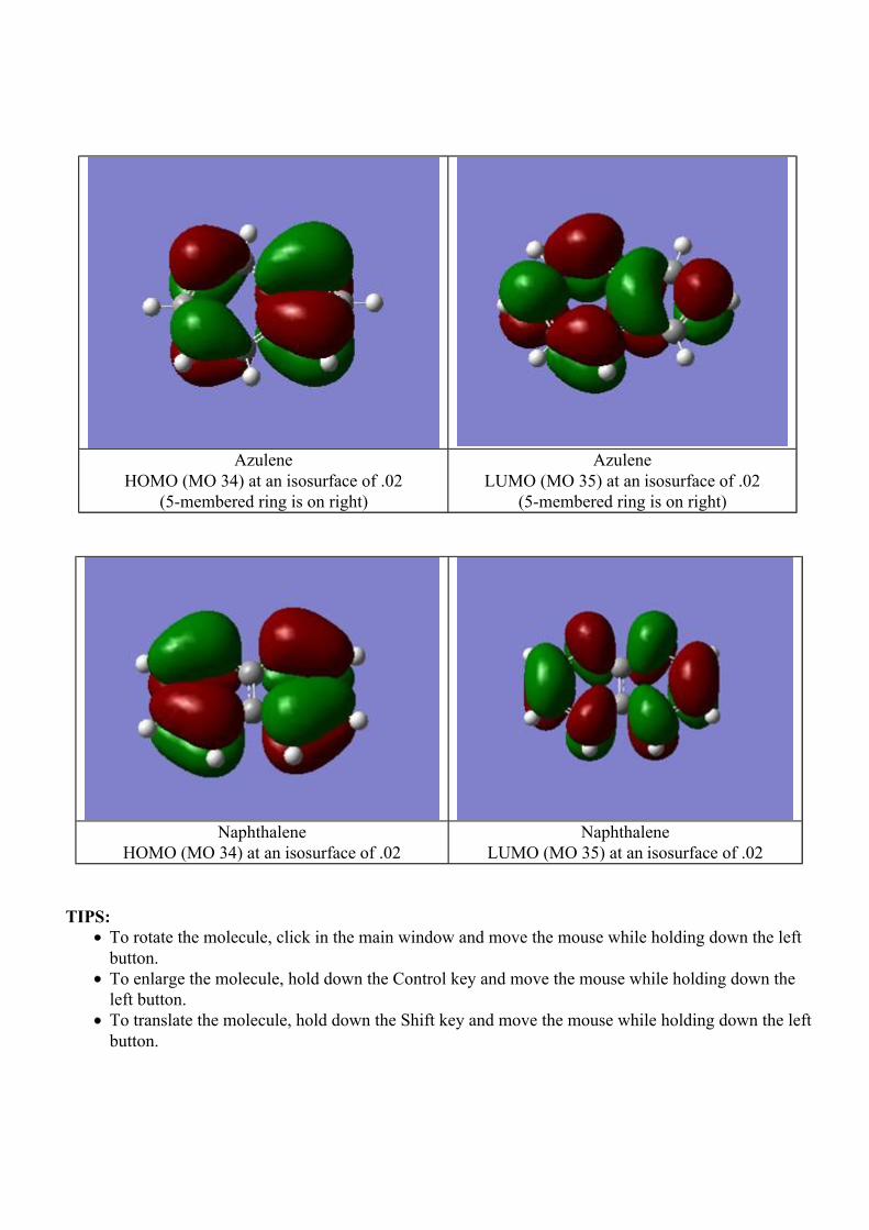
Naphthalene
HOMO (MO 34) at an isosurface of .02
Naphthalene
LUMO (MO 35) at an isosurface of .02
TIPS:
To rotate the molecule, click in the main window and move the mouse while holding down the left
button.
To enlarge the molecule, hold down the Control key and move the mouse while holding down the
left button.
To translate the molecule, hold down the Shift key and move the mouse while holding down the left
button.
Azulene
HOMO (MO 34) at an isosurface of .02
(5-membered ring is on right)
Azulene
LUMO (MO 35) at an isosurface of .02
(5-membered ring is on right)

Viewing Electrostatic Potential with GaussView(GaussView Version: 3.09)
Download The Files Associated With This Example
AzuleneInput
FileOutput File
Formatted
Checkpoint File
NaphthaleneInput
FileOutput File
Formatted
Checkpoint File
GaussView has the ability to view painted isosurfaces. These painted isosurfaces require two input files.
The isosurface of one value allows the second property to be displayed on it. This is particularly useful for
examining electrostatic potential. The electrostatic potential is mapped onto a particular value of the total
electron density. This can be done two ways in GaussView. The first way is to create the cube files using
the Gaussian CubeGen utility and then reading the cube file into GaussView. The second way is to have
GaussView generate the cube files internally from a previously created checkpoint file or formatted
checkpoint file.
Generating Formatted Checkpoint Files
When running the Gaussian calculation there are two ways in which you can get the desired formatted
checkpoint file.
As a keyword, enter formcheck. This will create a .FChk file when the Gaussian calculation is
complete.
1.
After the Gaussian calculation is complete, open Gaussian. Select Utilities|FormChk. In the dialog
box that appears, browse for the checkpoint file that was previously created. Select it. This will
create a formatted checkpoint file with the extension .fch that has the same name as the checkpoint
file. (This is the preferred method.)
2.
Generating Cube Files in Gaussian
After the Gaussian calculation is complete, open Gaussian.
Select Utilities|CubeGen.
The following dialog box appears:
Property[Density]? Density
Formatted Checkpoint File? C:\Filename.fch (note that you will need to specify the path to your
.fch file here)

Cube File [ ]? Filename.cub3 (this is the name of your cube file Cubegen will create)
Approximate Points per Side [O]? 40 (This puts roughly 40 points on each side of the cube,
giving it 403 points)
Header in cube file [H]? H (make sure to have a header so you can get the exact dimensions of
the cube file. T3D will require them)
Visualizing the Orbitals in GaussView
Select File|Open. Select the checkpoint file or formatted checkpoint file. Select OK.
Select Results|Surfaces. A Surfaces and Cubes window will appear.
Select the Cube Actions drop down menu. Select New Cube.
In the Kind box using the drop down menu select Total Density.
Leave all options as the default.
Select OK.
A line of data will appear in the Cubes Available box.
Select the Cube Actions drop down menu. Select New Cube.
In the Kind box using the drop down menu select ESP.
Leave all options as the default.
Select OK.
A second line of data will appear in the Cubes Available box.
Select an appropriate isosurface value (such as 0.020)
Adjust the isosurface value until you obtain a visualization of the difference densities that is
ideal.
Using the drop down button under Cubes Available, select the line that says Electron Density from
Total SCF Density.
Select the Surface Actions drop down menu. Select New Mapped Surface.
A Surface Mapping window appears. Select circle next to Use an Existing Cube. Under Cubes
Available, make sure that Electrostatic Potential from Total SCF Density is selected. Select OK.
A line of data will appear in the Surfaces Available box.
This will generate a graphical window with the mapped electrostatic potential displayed.
If the visualization is not ideal, select the Surface Actions drop down menu. Select Remove
Surface. Change the isosurface value. Select the Surface Actions drop down menu. Select
New Surface.
Repeat these steps until the visualization for the molecular orbital is ideal.
Using the drop down button under Cubes Available, select the line that says Electrostatic Potential
from Total SCF Density.
Select the Surface Actions drop down menu. Select New Surface.
A line of data will appear in the Surfaces Available box.
This will generate a graphical window with the molecular orbitals displayed
If the visualization is not ideal, select the Surface Actions drop down menu. Select Remove
Surface. Change the isosurface value. Select the Surface Actions drop down menu. Select
New Surface.
Repeat these steps until the visualization for the molecular orbital is ideal.
To change the display of the orbitals
Select View|Display Format.
Click on the Surface tab.
At the format drop down menu select either mesh, solid, or transparent.
The Z-Clip slider (min to max) can also be adjusted to alter the way the surface is viewed.
It may be used to remove the frontmost portions of the image to allow views into the interior
of the molecular display.

Azulene Electron Density – Viewed in GaussView Naphthalene Electron Density– Viewed in
GaussView
Azulene MEP – Viewed in GaussView Naphthalene MEP – Viewed in GaussView
TIPS:
To rotate the molecule, click in the main window and move the mouse while holding down the left
button.
To enlarge the molecule, hold down the Control key and move the mouse while holding down the left
button.
To translate the molecule, hold down the Shift key and move the mouse while holding down the left
button.

Viewing Gaussian Difference Densities with
GaussView(GaussView Version: 3.09)
Download The Files Associated With This Example
Ground State Input File Output File Cube File
Excited State 2 Input File Output File Cube File
Excited State 3 Input File Output File Cube File
Gaussview can be utilized to view the total electron density difference between ground and excited states.
The program reads the formatted checkpoint file or the cube file from a Gaussian calculation. This
example looks at several of the excited states of acrolein.
Generating Cube Files
For a Ground State Density
CIS/6-31G(d) density(SCF) cube=density NoSymm
At the end of input information
Blank line > filename_gs.cube > Blank line
For an Excited State Density
Input information located directly below last blank line from Ground State Density input
information
--link1--
%chk=filename.chk
# geom=allcheck guess(read, only) density(checkpoint,cis=n) cube=density
NoSymm
Where n represents the number for the excited state (example: n=2 for the second excited
state)
Blank line > filename_ex.cube > Blank line
Note: There are numerous ways to generate cube files. The method instructed above is simply the way
chosen for this particular demonstration. Also, the NoSymm keyword is included to ensure that Gaussian
does not reorient the molecule between calculations due to symmetry. If this occurs, the cube files could
have different coordinates and not line up properly when viewed.
Creating Difference Density Cube Files in Gaussian
Select Utilities|CubMan. A small window will appear.
Enter “su” for subtract at the initial prompt
This operation subtracts two cube files to produce a new cube file.
For the first input file type the name of the excited state cube file (example: filename_ex.cube)
Is the file formatted? Answer “y” for yes.
For the second input file type the name of the ground state cube file (example: filename_gs.cube)
Is the file formatted? Answer “y” for yes.
For the output file type in the name desired for the difference density output file (example:

filename_diffex.cube)
Should it be formatted? Answer “y” for yes.
Follow the above procedure for each of the excited states that you want to visualize the difference densities
for in GaussView.
Generating Formatted Checkpoint Files
When running the Gaussian calculation there are two ways in which you can get the desired formatted
checkpoint file.
1. As a keyword, enter formcheck. This will create a .FChk file when the Gaussian calculation is
complete.
2. After the Gaussian calculation is complete, open Gaussian. Select Utilities|FormChk. In the
dialog box that appears, browse for the checkpoint file that was previously created. Select it. This
will create a formatted checkpoint file with the extension .fch that has the same name as the
checkpoint file. (This is the preferred method.)
Visualizing Difference Densities in GaussView
GaussView can be used to read in two formatted checkpoint files or two cube files, take the difference, and
create an isosurface rendering of the result.
Select File|Open. Select the formatted checkpoint file for the excited state that you want to visualize
the difference density for in GaussView. Select OK.
Select Results|Surfaces. A Surfaces and Cubes window will appear.
Select the Cube Actions drop down menu. Select Load Cube. Find the cube file that represents the
difference density calculated with CubMan. Select OK.
A line of data will appear in the Cubes Available box.
Select an appropriate isosurface value (such as 0.004)
Adjust the isosurface value until you obtain a visualization of the difference densities that is ideal.
Select the Surface Actions drop down menu. Select New Surface.
A line of data will appear in the Surfaces Available box.
This will generate a graphical window with the molecule and difference density for your excited
state.
The blue represents where the electrons are coming from, and the purple represents where the
electrons are going.
If the visualization is not ideal, select the Surface Actions drop down menu. Select Remove
Surface. Change the isosurface value. Select the Surface Actions drop down menu. Select New
Surface.
Repeat these steps until the visualization for the difference density is ideal.

Acrolein Difference Density (Excited State 2 and Ground State) – Viewed in GaussView
Acrolein Difference Density (Excited State 3 and Ground State) – Viewed in GaussView
TIPS:
To rotate the molecule, click in the main window and move the mouse while holding down the left
button.
To enlarge the molecule, hold down the Control key and move the mouse while holding down the left
button.
To translate the molecule, hold down the Shift key and move the mouse while holding down the left
button.

Viewing Vibrational Frequencies in GaussView(GaussView Version: 3.09)
Download The Files Associated With This
Example
Input File Output File
The Vibrational Frequencies and IR Spectra of a molecule can be read by GaussView from any Gaussian
output file resulting from a Vibrational Frequencies calculation. This means either a file with the
extension .out or .log can be used.
Steps:
· Open GaussView
· Select File|Open
· Locate an output file from the Gaussian calculation (.out or .log)
· The molecule will appear in a new window
· Select Results|Vibrations
· A new window titled “Display Vibrations” will appear
· Select a Frequency and click Start
The molecule will now animate the vibrations associated the frequency selected. You can change the
frequency at any time during the animation by simply clicking on another frequency in the “Display
Vibrations” window.
There is no easy way to capture the vibrations from GaussView. However, there is the option of showing
displacement vectors, which displays arrows pointing the in direction each atom is moving. This could be
useful for displaying online or on paper to illustrate. To view displacement vectors, simply click the
“show displacement vectors” checkbox in the “Display Vibrations” window mentioned previously.

Picture of N,N-dimethylacetamide with displacement vectors
Similarly, The infrared spectra can be viewed by clicking the “Spectrum” button in the “Display
Vibrations” window. Sections of the IR Spectrum can be enlarged by selecting the IR Spectrum window,
the clicking and dragging a box around the region of interest. After selecting a region, you can return to
the full spectrum by right clicking in the window and selecting “Zoom Out”

Viewing NMR Tensors with GaussView(GaussView Version: 3.09)
Download The Files Associated With This Example
Ethane: Input OutputFormatted
Checkpoint File
Ethene: Input OutputFormatted
Checkpoint File
Ethyne: Input OutputFormatted
Checkpoint File
NMR Tensors can be viewed in GaussView if you have generated cube files from either the checkpoint file
or the formatted checkpoint file. The process for doing so is described below:
The first step in this process is to format the checkpoint file from the NMR Gaussian job.
In Gaussian 03, select Utilities|FormChk
Using the File Browser that opens, locate the checkpoint file from the NMR calculation and click OK
A command line window will open, and the checkpoint file will be formatted
Next you must use this file to generate Cube Files
Open GaussView
Select File|Open
Open the formatted checkpoint file resulting from the Gaussian NMR calculation
Select Results|Surfaces
A window titled Surfaces and Cubes will spawn
Click on the Cube Actions pulldown and select “New Cube”
Kind: Current Density
Shielding Tensor Component: Z
Grid: Medium
A command line will open in the background and run Cubegen, a Gaussian utility, to create the cube
file which is now available in the list of available cubes in the “Surfaces and Cubes” window
The next two cubes will be Shielding Density cubes. Creating Shielding Density cubes requires that
you specify an atom. To help you choose the correct atom number, you can select View|Display
Format and under the General tab, click “Show Tags”. This will number each atom for you.
First Cube
Kind: Shielding Density
Shielding Tensor Component: ZZ
Grid: Medium
Atom: 1 (Carbon)
Second Cube
Kind: Shielding Density
Shielding Tensor Component: ZZ
Grid: Medium
Atom: 3 (Hydrogen)
You can save the cube files by selecting them in the pulldown menu and then going to the Cube
Actions pulldown menu and selecting “Save Cube”

Now you are ready to view the newly generated cube files
To show an isosurface of the current density, select the Current Density cube under the Available
Cubes heading, and type an isosurface value at the bottom of the window. Then click on the Surface
Actions pulldown menu and select “New Surface”. The isosurface of current density will appear.
Once you have an appropriate value for the isosurface, pull down the Surface Actions pulldown and
either hide or remove that surface.
To Map Shielding Density on the Current Density Isosurface
Select the Current Density Cube file from the
available cubes pulldown menu, and then enter an
isosurface value at the bottom of the window. Go to
the Surface Actions pulldown menu and select
“New Mapped Surface”. Choosing the Current
Density cube before selecting this option signifies
that the Current Density isosurface is the surface
that will be use to map on.
Select “New Mapped Surface” and then select one of the Shielding Density cube files from the
pulldown menu. Click OK
The Shielding Density will now map onto the Current Density Isosurface. There will be a color map
at the top of the molecule window. You can adjust the range of the color map by changing the values
in either end of the color map.
Note: In the pictures below, the negative values represent deshielding while the positive values represent shielding
Ethane
Shielding Density as seen by Nucleus 3 (H) in the ZZ direction mapped
between the values of -.05 to .1 on the Current Density=Z isosurface at
a value of .00004
Ethene
Shielding Density as seen by Nucleus 1 (C) in the YY direction
mapped between the values of -1 to 1 on the Current Density=1
isosurface at a value of .0003

Ethene
Shielding Density seen by Nucleus 3 (H) in the ZZ
direction mapped between the values of -.3 to .3 on
the Current Density=Z isosurface at a value of .0002
Ethyne
Shielding Density seen by Nucleus 1 (C) in the
ZZ direction mapped between values of -.5 to .5
onto the Current Density=Z isosurface at a value
of .0004

Viewing a Reaction Path with GaussView(GaussView Version: 3.09)
Download the Files Associated With This Example
Input File Output FileFormatted Checkpoint
File
Gaussview can be utilized to view the reaction pathway. The program reads the formatted checkpoint file
or the output file from a Gaussian calculation. This example looks at the reaction pathway of H2 and
acetone.
Generating Formatted Checkpoint Files
When running the Gaussian calculation there are two ways in which you can get the desired formatted
checkpoint file.
1. As a keyword, enter formcheck. This will create a .FChk file when the Gaussian calculation is
complete.
2. After the Gaussian calculation is complete, open Gaussian. Select Utilities|FormChk. In the
dialog box that appears, browse for the checkpoint file that was previously created. Select it. This
will create a formatted checkpoint file with the extension .fch that has the same name as the
checkpoint file. (This is the preferred method.)
Preparing to Visualize Reaction Path
Create reactants, products, and an educated guess at the transition structure
Run these through a Gaussian optimization job
Use additional keywords opt (QST3, CalcFC)
QST3 is a search for a transition structure
This option requires the reactant, product, and initial transition structure
structures as input
CalcFC specifies that the force constants be computed at the first point
Create a formatted checkpoint file
Next, run these through a Gaussian frequency job
Create a formatted checkpoint file
Finally, run these through a Gaussian Reaction Path job (IRC)
Use additional keywords IRC (Maxpoints=24, RCFC, phase=(1,2)) NOSYMM
IRC requests that a reaction path be followed
Maxpoints represents the number of points along the reaction path to be examined
RCFC specifies that the computed force constants in Cartesian coordinates from a
frequency calculation be read from the checkpoint file
Phase defines the phase for the transition vector
If two atom numbers are given, the coordinate is a bond stretch between the two
atoms
Create a formatted checkpoint file
Note: IRC Calculations require initial force constants to proceed. These must be provided to the

calculation in some way. The usual method is to save the checkpoint file from the preceding frequency
calculation (used to verify that the optimized geometry to be used in the IRC calculation is in face a
transition state).
Visualizing Reaction Paths in GaussView
Select File|Open. Select either the formatted checkpoint file or the output file that was created
from the IRC Calculation. Select OK.
A window will appear with the selected structure displayed with the option of showing all the steps
along the reaction pathway.
The formatted checkpoint file will have 1 of 49 steps of the reaction pathway
The output file will have 1 of 48 steps of the reaction pathway
To view each of the steps along the reaction pathway, simply click on the up or down arrow located
next to the first number.
To view a timeline of all the steps along the reaction pathway, click on the button that shows a split
screen with two molecules located next to the second number (the one that is fixed). The button
will now only show one molecule. To view only one step at a time, click on the same button.
To view a slideshow of all the stops along the reaction pathway, click on the green button located
next to the first number. The green button will turn into a red “X”. To stop the slideshow, click on
the red “X”.
Reaction Pathway Timeline – Viewed in GaussView
TIPS:
To rotate the molecule, click in the main window and move the mouse while holding down the left
button.
To enlarge the molecule, hold down the Control key and move the mouse while holding down the
left button.
To translate the molecule, hold down the Shift key and move the mouse while holding down the left
button.

Webtools
Mainpage of the molecule database
Molecule editor interface

Topic editor interface
Visualization of the molecular database

Molecular Design and Quantum Chemistry
Appendix
To solve exercises we used Gaussian03 ab-initio program package. Other ab-initio programs and free demos can be found in the next location
http://www.theochem.uni-stuttgart.de/theolinks/links.html below the Program Packages and Documentations Ab initio program packages titles
Appendix 1
Problem
Compute the energy profile of the concreted (A) and stepwise (B) mechanism of reaction between metil-cloride and Brom ion.
Solution of SN2 (concreted) reaction.
To solve this problem we use Gaussian 03 and gview programs. As we calculate the energy in gas phase the energy profile is similar to the next
TS
C2
E
reaction coordinate
C1
First we have to optimize the starting complex (C1) and product complex (C2). One of the input files is below
%chk=SNopt.chk %mem=6MW %nproc=1 #p opt hf/3-21g optimization at 3-21g basis set Metilklorid - bromide ion kiindulasi complex(C1) optimizacioja note

Molecular Design and Quantum Chemistry -1 1 charge -1, multiplicity singlet C 0.61552264 0.78757807 0.54621719 atomic coordinates in Cartesian frame H 0.97217707 -0.22123193 0.54621719 H 0.97219548 1.29197626 1.41986870 H 0.97219548 1.29197626 -0.32743431 Cl -1.14447736 0.78759976 0.54621719 Br 3.84149447 0.83548548 0.70019980 Then we make a redundant coordinate between the Brom ion and carbon atom of metil-cloride. During the optimization we increase the distance between the two atoms with 0.01Å in each step. %chk= %mem=6MW %nproc=1 #p opt=modredundant hf/3-21g geom=connectivity optimization at 3-21g basis set SN reakció scan a szén-bromion tavolsag csökkentésével -1 1 C atomic coordinates in Z-matrix form H 1 B1 H 1 B2 2 A1 H 1 B3 2 A2 3 D1 Cl 1 B4 4 A3 3 D2 Br 1 B5 4 A4 3 D3 B1 1.06717105 B2 1.06718052 B3 1.06716759 B4 1.99526909 B5 3.11779504 A1 114.18106258 A2 114.19157479 A3 104.19767784 A4 75.81809217 D1 133.94956808 D2 113.03179128 D3 -66.94632404 1 2 1.0 3 1.0 4 1.0 2 3 4 5 6 redundant parameters: Bond between atom no.6 and 1 step no.150 B 6 1 S 150 -0.010000 step -0.010000Å
You can see the results in the gwiev. You have to choose in the open dialog box read intermediate geometries and open the out file. If in the results dialog box you choose the scan option you will get a diagram of C-Br distance versus Energy of molecule. The diagram is false after the second minima, because the C-Br distance too short, so we have to calculate with other redundant coordinate.

Molecular Design and Quantum Chemistry
Appendix 2
Problem: Use Gaussian X program package to compute the dipole momentum of following species: CH4, C2H6, C3H8, Butan (4 conformers), MeCl, MeBr, MeF, MeOH, MeSH, MeNH2, MeMgCl.
Solution: Input file for methane:
%chk=metan.chk
%mem=6MW
%nproc=1
#p opt hf/3-21g
Methan dipole moment
0 1
C
H 1 B1
H 1 B2 2 A1
H 1 B3 3 A2 2
D1
H 1 B4 3 A3 2
D2
B1 1.07000000
B2 1.07000000
B3 1.07000000
B4 1.07000000
A1 109.47120255
A2 109.47125080
A3 109.47121829
D1 -119.99998525
D2 120.00000060
Results:
Species Computed
Metane 0 debey
Ethane 0 debey
Propane 0 debey
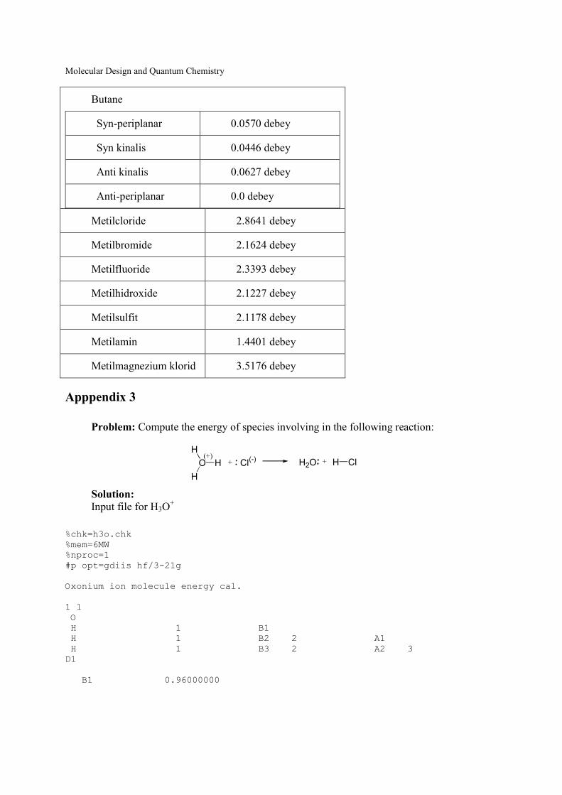
Molecular Design and Quantum Chemistry
Butane
Syn-periplanar 0.0570 debey
Syn kinalis 0.0446 debey
Anti kinalis 0.0627 debey
Anti-periplanar 0.0 debey
Metilcloride 2.8641 debey
Metilbromide 2.1624 debey
Metilfluoride 2.3393 debey
Metilhidroxide 2.1227 debey
Metilsulfit 2.1178 debey
Metilamin 1.4401 debey
Metilmagnezium klorid 3.5176 debey
Apppendix 3
Problem: Compute the energy of species involving in the following reaction:
Cl(-) H2O H Cl
(+)O
H
H
H ++
Solution:
Input file for H3O+
%chk=h3o.chk
%mem=6MW
%nproc=1
#p opt=gdiis hf/3-21g
Oxonium ion molecule energy cal.
1 1
O
H 1 B1
H 1 B2 2 A1
H 1 B3 2 A2 3
D1
B1 0.96000000

Molecular Design and Quantum Chemistry B2 0.96000000
B3 0.96000000
A1 109.47122063
A2 109.47122063
D1 120.00000000
Species Energy in a.u.
H3O+ -75.89122771
Cl- -457.35358538
H2O -75.58580978
HCl -457.86943112