Molecular Dynamics Department of Computer Science and Engineering Prof. Jesus Izaguirre Alice Ko

Molecular Dynamics

Department of Computer Science and Engineering

Prof. Jesus Izaguirre

Alice Ko

Outline

1. What is biomolecular modeling?

2. Historical perspective

3. Theory and experiments

4. Simulation procedures

5. MDSimAid

What is biomolecular modeling?

• Application of computational models to understand the structure, dynamics, and thermodynamics of biological molecules

• The models must be tailored to the question at hand: Schrodinger equation is not the answer to everything! Reductionist view bound to fail!

• This implies that biomolecular modeling must be both multidisciplinary and multiscale

Historical Perspective

1. 1946 MD calculation

2. 1960 force fields

3. 1969 Levinthal’s paradox on protein folding

4. 1970 MD of biological molecules

5. 1971 protein data bank

a. 1998 ion channel protein crystal structure

b. 1999 IBM announces blue gene project

Theoretical Foundations

1. Born-Oppenheimer approximation (fixed nuclei)2. Force field parameters for families of chemical

compounds3. System modeled using Newton’s equations of

motion4. Examples: hard spheres simulations (alder and

Wainwright, 1959); Liquid water (Rahman and Stillinger, 1970); BPTI (McCammon and Karplus); Villin headpiece (Duan and Kollman, 1998)

Study of Dynamics I

• The computational study of atomic fluctuations in BPTI and other proteins has shown that :– Directional character of active-site fluctuations

in enzymes contributes to catalysis– Small amplitude fluctuations are “lubricant”– It may be possible to extrapolate from short

time fluctuations to larger-scale protein motions

Study of Dynamics II

• Collective motions particularly important for biological function, e.g., displacements for transition from inactive to active – Extended nature of these motions makes them

sensitive to environment: great difference between vacuum and solution simulations

– Collective motions transmit external solvent effects to protein interior

Study of Dynamics III• For the transport protein hemoglobin there are

several important motions:– Oxygen binding produces tertiary structural change

– A quaternary structural change from deoxy (low oxygen affinity) to oxy configuration takes place. This transmits information over a long distance

– From the X-ray deoxy and oxy structures, a stochastic reaction path has been found. Detailed ligand binding has been performed using MD. A statistical mechanical model has provided coupling between these two processes

Study of Dynamics IV

• For the related storage protein, myoglobin:– Fluctuations in the globin are essential to

binding: the protein matrix in X-ray is so tightly packed that there is no low energy path for the ligand to enter or leave the heme pocket

– Only through structural fluctuations can the barriers be lowered sufficiently

– Demonstrated through energy minimization and molecular dynamics

Study of Dynamics VI

• Three open problems are the following:1. Ion channel gating: highly correlated fluctuations are

likely to be of great importance. Long time dynamics problem

2. Flexible docking: for MMP, enzymes, etc., fluctuations enter into thermodynamics and kinetic of reactions. Sampling problem

3. Protein folding: too complicated for full treatment but for smallest proteins, beyond current methodology. Coarsening problem

An Introduction to Molecular Dynamics Simulations

Macroscopic properties are often determined by molecule-level behavior.

Quantitative and/or qualitative information about macroscopic behavior of macromolecules can be obtained from simulation of a system at atomistic level.

Molecular dynamics simulations calculate the motion of the atoms in a molecular assembly using Newtonian dynamics to determine the net force and acceleration experienced by each atom. Each atom i at position ri, is treated as a point with a mass mi and a fixed charge qi.NOTE: This material is courtesy of Klaus Schulten, www.ks.uiuc.edu

Steps in Molecular Dynamics Simulations

1) Build realistic atomistic model of the system

2) Simulate the behavior of your system over time using specific conditions (temperature, pressure, volume, etc)

3) Analyze the results obtained from MD and relate to macroscopic level properties

What you need to know to build a realistic atomistic model of your system

• What is a forcefield?

• How to prepare your system for MD?

• What specific conditions (temperature, pressure, volume, etc) will be used in MD?

What is a Forcefield?

To describe the time evolution of bond lengths, bond angles and torsions, also the nonbond van der Waals and elecrostatic interactions between atoms, one uses a forcefield.The forcefield is a collection of equations and associated constants designed to reproduce molecular geometry and selected properties of tested structures.

In molecular dynamics a molecule is described as a series of charged points (atoms) linked by springs (bonds).

Energy Terms Described in the CHARMm forcefield

Bond Angle

Dihedral Improper

Energy Functions

Ubond = oscillations about the equilibrium bond lengthUangle = oscillations of 3 atoms about an equilibrium angleUdihedral = torsional rotation of 4 atoms about a central bondUnonbond = non-bonded energy terms (electrostatics and Lenard-Jones)

Topology and Parameter Files

Topolgy files contain:• atom types are assigned to identify different elements and different molecular orbital environments• charges are assigned to each atom • connectivities between atoms are established

Parameter files contain:• force constants necessary to describe the bond energy, angle energy, torsion energy, nonbonded interactions (van der Waals and electrostatics)• suggested parameters for setting up the energy calculations

Example of Topology File

MASS HS 1.0080 ! thiol hydrogen MASS C 12.0110 ! carbonyl C, peptide backbone MASS CA 12.0110 ! aromatic C........ (missing data here)!----------------------------------------------------------- AUTOGENERATE ANGLES=TRUE DIHEDRALS=TRUE END!----------------------------------------------------------- RESIDUE ALA

GROUP ATOM N TYPE=NH1 CHARGE= -.4700 END ! | ATOM HN TYPE=H CHARGE= .3100 END ! N--HN ATOM CA TYPE=CT1 CHARGE= .0700 END ! | HB1 ATOM HA TYPE=HB CHARGE= .0900 END ! | / GROUP ! HA-CA--CB-HB2 ATOM CB TYPE=CT3 CHARGE= -.2700 END ! | \ ATOM HB1 TYPE=HA CHARGE= .0900 END ! | HB3 ATOM HB2 TYPE=HA CHARGE= .0900 END ! O=C ATOM HB3 TYPE=HA CHARGE= .0900 END ! | GROUP ! ATOM C TYPE=C CHARGE= .5100 END ATOM O TYPE=O CHARGE= -.5100 END !END GROUP BOND CB CA BOND N HN BOND N CA BOND O C BOND C CA BOND CA HA BOND CB HB1 BOND CB HB2 BOND CB HB3 DONOR HN N ACCEPTOR O C END {ALA }

CA CB

N

HN

HAC

O

HB3

HB1

HB2

!BOND PARAMETERS: Force Constant, Equilibrium Radius BOND C C 600.000 {SD=.022} 1.335 ! ALLOW ARO HEM BOND CA CA 305.000 {SD=.031} 1.375 ! ALLOW ARO

!ANGLE PARAMETERS: Force Constant, Equilibrium Angle, Urie-Bradley Force Const., U.-B. equilibrium (if any) ANGLE CA CA CA 40.00 {SD=.086} 120.0000 UB 35.000 2.416 ANGLE CP1 N C 60.00 {SD=.070} 117.0000 ! ALLOW PRO

!DIHEDRAL PARAMETERS: Energy Constant, Periodicity, Phase Shift, Multiplicity DIHEDRAL C CT2 NH1 C 1.60 {SD=.430} 1 180.0000 ! ALLOW PEP DIHEDRAL C N CP1 C .80 {SD=.608} 3 .0000 ! ALLOW PRO PEP

!IMPROPER PARAMETERS: Energy Constant, Periodicity(0), Phase Shift(0)! Improper angles are introduced for PLANARITY maintaining IMPROPER HA C C HA 20.00 {SD=.122} 0 .0000 ! ALLOW PEP POL ARO IMPROPER HA HA C C 20.00 {SD=.122} 0 180.0000 ! ALLOW PEP POL ARO

! -----NONBONDED-LIST-OPTIONS------------------------------- CUTNB= 13.000 TOLERANCE= .500 WMIN= 1.500 ATOM INHIBIT= .250! -----ELECTROSTATIC OPTIONS-------------------------------- EPS= 1.000 E14FAC= 1.000 CDIELECTRIC SHIFT! -----VAN DER WAALS OPTIONS-------------------------------- VSWITCH! -----SWITCHING /SHIFTING PARAMETERS----------------------- CTONNB= 10.000 CTOFNB= 12.000! -----EXCLUSION LIST OPTIONS------------------------------- NBXMOD= 5! ------------! EPS SIGMA EPS(1:4) SIGMA(1:4)

NONBONDED C .1100 4.0090 .1100 4.0090 ! ALLOW PEP POL ARO NONBONDED CA .0700 3.5501 .0700 3.5501 ! ALLOW ARO

Example ofParameter File





Preparing Your System for MD (1)

What you have up to now: • pdb file, • topology file• parameter file

What you need next: a program capable of reading and manipulating this information

Programs: X-PLOR, CHARMm, NAMD2, AMBER, GROMOS, EGO, PROTOMOL, etc.

Preparing Your System for MD (2)Minimization

The energy of the system can be calculated using the forcefield. The conformation of the system can be altered to find lower energy conformations through a process called minimization.

Minimization algorithms:• steepest descent (slowly converging – use for highly restrained systems• conjugate gradient (efficient, uses intelligent choices of search direction – use for large systems)• BFGS (quasi-newton variable metric method)• Newton-Raphson (calculates both slope of energy and rate of change)

Conformational change

Energy

Preparing Your System for MD (3)Solvation

Biological activity is the result of interactions between molecules and occurs at the interfaces between molecules (protein-protein, protein-DNA, protein-solvent, DNA-solvent, etc).

Why model solvation?• many biological processes occur in aqueous solution• solvation effects play a crucial role in determining molecular conformation, electronic properties, binding energies, etc

How to model solvation?• explicit treatment: solvent molecules are added to the molecular system • implicit treatment: solvent is modeled as a continuum dielectric





Molecular Dynamics –what does it mean?

MD = change in conformation over time using a forcefield

Conformational change

EnergyEnergy supplied to the minimized system at the start of the simulation

Conformation impossible to access through MD

MD: Verlet Method

Newton’s equation represents a set of N second order differential equations which are solved numerically at discrete time steps to determine the trajectory of each atom.

Advantage of the Verlet Method: requires only one force evaluation per timestep

Energy function:

used to determine the force on each atom:

Molecular Dynamics Ensembles

Constant energy, constant number of particles (NE)

Constant energy, constant volume (NVE)

Constant temperature, constant volume (NVT)

Constant temperature, constant pressure (NPT)

Choose the ensemble that best fits your system and start the simulations

Happy computing!

Steps in Molecular Dynamics Simulations

1) Build realistic atomistic model of the system

2) Simulate the behavior of your system over time using specific conditions (temperature, pressure, volume, etc)

3) Analyze the results obtained from MD and relate to macroscopic level properties

Example: MD Simulations of the K+ Channel Protein

Ion channels are membrane - spanning proteins that form a pathway for the flux of inorganic ions across cell membranes.

Potassium channels are a particularly interesting class of ion channels, managing to distinguish with impressive fidelity between K+ and Na+ ions while maintaining a very high throughput of K+ ions when gated.

Setting up the system (1)

• retrieve the PDB (coordinates) file from the Protein Data Bank

• use topology and parameter files to set up the structure

• add hydrogen atoms using X-PLOR

• minimize the protein structure using NAMD2

Setting up the system (2)

Simulate the protein in its natural environment: solvated lipid bilayer

lipids

Setting up the system (3)Inserting the protein in the lipid bilayer

gaps

Automatic insertion into the lipid bilayer leads to big gaps between the protein and the membrane => long equilibration time required to fill the gaps.Solution: manually adjust the position of lipids around the protein

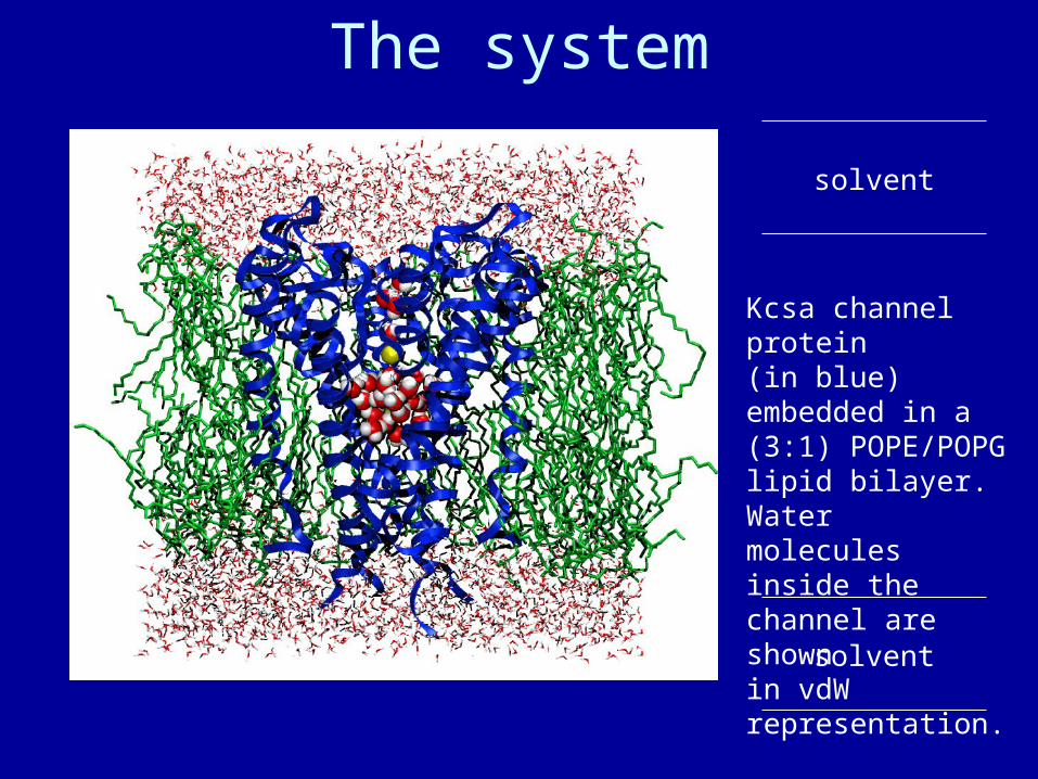
The system

solvent

solvent

Kcsa channel protein(in blue) embedded in a (3:1) POPE/POPGlipid bilayer. Watermolecules inside thechannel are shownin vdW representation.

Summary of simulations:• protein/membrane system contains 38,112 atoms, including 5117 water molecules, 100 POPE and 34 POPG lipids, plus K+ counterions• CHARMM26 forcefield• periodic boundary conditions, PME electrostatics• 1 ns equilibration at 310K, NpT• 2 ns dynamics, NpT

Program: NAMD2

Platform: Cray T3E (Pittsburgh Supercomputer Center)

Simulating the system:Free MD

MD Results

RMS deviations for the KcsA protein and its selectivity filer indicate that the protein is stable during the simulation with the selectivity filter the most stable part of the system.

Temperature factors for individual residues in the four monomers of the KcsA channel protein indicate that the most flexible parts of the protein are the N and C terminal ends, residues 52-60 and residues 84-90. Residues 74-80 in the selectivity filter have low temperature factors and are very stable during the simulation.

Simulating the system:Steered Molecular Dynamics (SMD)

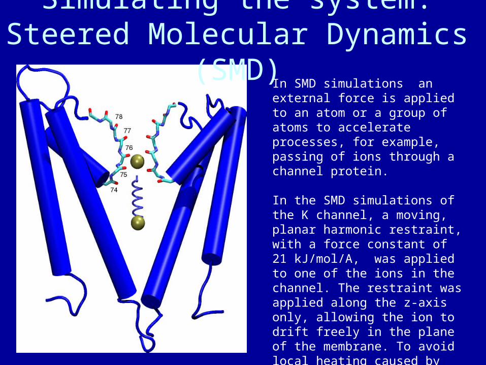
In SMD simulations an external force is applied to an atom or a group of atoms to accelerate processes, for example, passing of ions through a channel protein.

In the SMD simulations of the K channel, a moving, planar harmonic restraint, with a force constant of 21 kJ/mol/A, was applied to one of the ions in the channel. The restraint was applied along the z-axis only, allowing the ion to drift freely in the plane of the membrane. To avoid local heating caused by applied external forces, all heavy atoms were coupled to a Langevin heat bath with a coupling constant of 10/ps.

SMD Results

After 400 ps, the leading ion moves into chamber 77. The intervening chamber is left unfilled by the trailing ion for ~ 100 ps. At 500 ps, the trailing ion moves into chamber 76 behind the leading ion, overcoming its attraction for Thr75 and Val76 but moving into a more favorable interaction position with Gly77. The trailing ion overcomes an energy barrier of ~50 kJ/mol due to interactions with the backbone. Just after this trailing ion moves in, PRO3 isomerizes to bring the carbonyl oxygen of Gly77 into favorable alignment with both potassium ions. The isomerization stabilizes the backbone by ~30 kJ/mol. Around 795-800 ps, the two ions make a concerted transition to the next pair of chambers. Almost simultaneously, Gly77 carbonyl oxygen swings back to its former position.

Steered ion 78777675

MD –Shortcomings• Quality of the forcefield

• Size and Time – atomistic simulations can be performed only for systems of a few tenths of angstroms on the length scale and for a few nanoseconds on the time scale

• Conformational freedom of the molecule – the number of possible conformations a molecule can adopt is enormous, growing exponentially with the number or rotatable bonds.

• Only applicable to systems that have been parameterized

• Connectivity of atoms cannot change during dynamics – no chemical reactions

Multiple time stepping (MTS):Verlet-I/r-RESPA/Impulse

F_fast

F_slow

Grubmuller (1989)Grubmuller, Heller, Windemuth & Schulten (1991)Tuckerman, Berne & Martyna (1992)

1. Fast/slow force splitting (Grubmuller ’89, ’91, and Tuckerman ’92)2. Use switching functions on potentials/forces (Tuckerman ’92)

F_fastF_fastF_fastF_fastF_fast F_fastTime

F_slow F_slowTime

Time step barrier

• Even for MTS, theory and experiment indicate that energy growth occur unless

longest t < 1/3 period.

• Note: This resonance is purely numerical artifact, natural resonance only happens at

longest t = period.

Ma, Izaguirre & Skeel (2001)

.

DM computes dynamics correctly: self-diffusion coefficients

Type t(fs)

t(fs)

(ps-1)

D(10-5cm2/s)

= 10-7

D(10-5cm2/s)

= 10-12

LF - 1 - 3.64 ± 0.05 3.71 ± 0.02

VI 4 1 - 3.62 ± 0.06 3.77 ± 0.09

DM 16 2 4.05 3.65 ± 0.05 3.70 ± 0.05

Table 1. Diffusion coefficient computed using different methods for 400 ps simulation of 141 water molecules, PBC, Ewald

DM provides substantial speedup

Type t(fs)

t(fs)

(ps-1)

Time and Speedup

(hours, = 10-7)

Time and Speedup

(hours, = 10-12)

LF - 1 - 49.83, 1.00 68.28, 1.00

VI 4 1 - 18.68, 2.67 23.50, 2.91

DM 16 2 4.05 10.09, 4.94 11.40, 5.99

Table 2. Speedup comparisons for different methods for 400 ps simulation of 141 water molecules, PBC, Ewald

Summary of Dissipative MOLLY

• Time reversible, momentum preserving and temperature preserving MTS integrator for molecular dynamics.

• Computes dynamics correctly using step sizes up to 16 fs.

• Substantial speedup for sequential executions.

Simulation Procedure Overview

Simulation Procedures

• Setup1. PDB file

– Protein Databank (http://www.rcsb.org/pdb/)

2. PSF file– Generated specifically for the molecule

– Contains the detailed composition and connectivity of the molecule(s) of interest

http://www.rcsb.org/pdb/






• Setup1. Topology file

– information for putting molecules together, such as what atoms are to be used, which of these atoms are bonded to each other, and the sets of atoms that form bond angles

2. Parameter file– physical parameters (force constants, van der

Waals forces, bonds, angles, etc.)


• Solvation– Create water box or shell to enclose the

molecule

• Minimization– Minimize the energy of the system in order to

reach the most favorable configuration


• Heating– Initial velocities are assigned at a

low temperature. Periodically, new velocities are assigned at a slightly higher temperature and the simulation is allowed to continue. This is repeated until the desired temperature is reached.


• Equilibration– The point of the equilibration phase

is to run the simulation until the structure, pressure, temperature and energy become stable with respect to time.


• Dynamics– Normal/Periodic boundary condition– Single/Multiple time stepping– Integrators– Electrostatics


• Analysis– Mean energy

– RMS difference between two structures


• Visualization– molecular graphics programs

• VMD

• InsightII

MDSimAid

• Purpose– To help setup molecular simulations– To avoid being overwhelmed by the amount of

technical details– To choose optimal parameters based on desire

accuracy

MDSimAid

• Python interpreter

• CHARMM– Bob.nd.edu– http://yuri.harvard.edu/

• ProtoMol– Bob.nd.edu– www.nd.edu/~lcls/ProtoMol

http://yuri.harvard.edu/







http://www.nd.edu/~lcls/ProtoMol

MDSimAid

• PSF generation

• Solvation

• Minimization

• Heating

• Equilibration

• Dynamics

Future Work

• Extend to multiple time stepping methods

• Multiple ensembles (currently NVE)

• Interface to more programs (NAMD, CHARMm – for dynamics)

• Collaborations, incorporate suggestions

• GUI

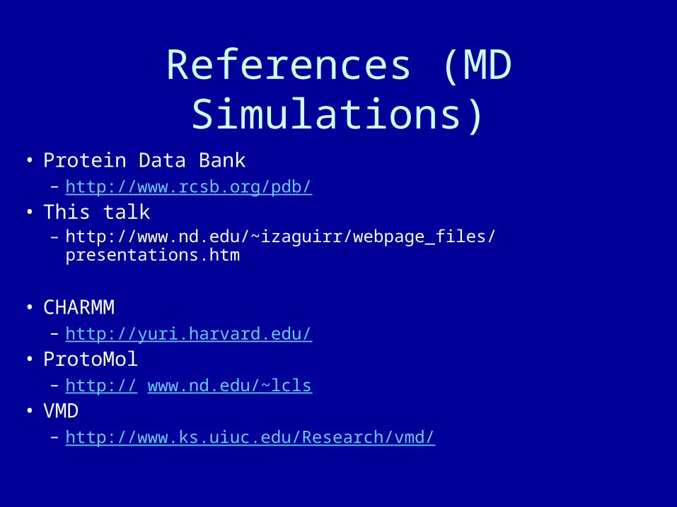
References (MD Simulations)

• Protein Data Bank– http://www.rcsb.org/pdb/

• This talk– http://www.nd.edu/~izaguirr/webpage_files/presentations.htm

• CHARMM– http://yuri.harvard.edu/

• ProtoMol– http:// www.nd.edu/~lcls

• VMD– http://www.ks.uiuc.edu/Research/vmd/














http://www.nd.edu/~lcls

http://www.nd.edu/~lcls

http://www.ks.uiuc.edu/Research/vmd/

References (MTS)[1] E. Barth and T. Schlick. Extrapolation versus impulse in multiple-time-stepping schemes: Linear analysis and applications to Newtonian and

Langevin dynamics. J. Chem. Phys., 1997. In press.[2] A. Brunger, C. B. Brooks, and M. Karplus, Stochastic boundary conditions for molecular dynamics simulations of ST2 water, Chem. Phys. Lett. 105

(1982), 495-500.[3] G. Besold, I. Vattulainen, M. Kartunnen, and J. M. Polson. Towards better integrators for dissipative particle dynamics simulations. Physical Review

E, 62(6):R7611–R7614, Dec. 2000.[4] B. Garcya-Archilla, J. M. Sanz-Serna, and R. D. Skeel. The mollified impulse method for oscillatory differential equations. In D. F. Griffiths and G.

A. Watson, editors, Numerical Analysis 1997, pages 111–123, Pitman, 1998[5] R. D. Groot and P. B. Warren. Dissipative particle dynamics: Bridging the gap between atomistic and mesoscopic simulation. J. Chem. Phys.,

107(11):4423–4435, Sep 15 1997.[6] H. Grubmuller. Dynamiksimulation sehr grober Makromoleckule auf einem Parallelrechner, Master’s thesis, Physik-Dept. der Tech. Univ. Munchen,

Munich, 1989[7] H. Grubmuller, H. Heller, A. Windemuth, and K. Schulten, Generalized Verlet algorithm for efficient molecular dynamics simulations with long

range interactions, Molecular Simulations 6 (1991), 121-142.[8] J. A. Izaguirre, D. P. Catarello, J.M.Wozniak, and R. D. Skeel. Langevin stabilization of molecular dynamics. J. Chem. Phys., 114(5):2090–2098,

Feb. 1, 2001.[9] J. A. Izaguirre, Q. Ma, T. Matthey, J. Willcock, T. Slabach, B. Moore, and G. Viamontes. Overcoming instabilities in verlet-i/r-RESPA with the

mollified impulse method. In T. Schlick, editor, Proceedings of International Workshop on Methods for Macromolecular Modeling, volume 24, Berlin-New York, 2002. Springer Verlag. In press, preprint at http://www.nd.edu/˜izaguirr/papers/newM3paper.pdf.

[10] J. A. Izaguirre, S. Reich, and R. D. Skeel. Longer time steps for molecular dynamics. J. Chem. Phys., 110(19):9853–9864, May 15, 1999.[11] L. Kale, R. Skeel, M. Bhandarkar, R. Brunner, A. Gursoy, N. Krawetz, J. Phillips, A. Shinozaki, K. Varadarajan, and K. Schulten. NAMD2: Greater

scalability for parallel molecular dynamics. J. Comp. Phys., 151:283–312, 1999.[12] Q. Ma, J. A. Izaguirre, and R. D. Skeel. Verlet-I/r-RESPA is limited by nonlinea instability. Submitted to SIAM Journal on Scientific Computing,

2001.[13] I. Pagonabarraga and D. Frenkel. Dissipative particle dynamics for interacting systems. J. Chem. Phys., 115(11):5015–5026, September 15 2001.[14] I. Pagonabarraga, M. Hagen, and D. Frenkel. Self-consistent dissipative particle dynamics algorithm. Europhysics Letters, 42(4):377–382, May 15

1998.[15] R. D. Skeel. Integration schemes for molecular dynamics and related applications. In M. Ainsworth, J. Levesley, and M. Marletta, editors, The

Graduate Student’s Guide to Numerical Analysis, SSCM, pages 119-176. Springer-Verlag, Berlin, 1999[16] R. D. Skeel & J. A. Izaguirre. An impulse integrator for Langevin dynamics, submitted, 2002.[17] M. Tuckerman, B. J. Berne, and G. J. Martyna, Reversible multiple time scale molecular dynamics, J. Chem. Phys 97 (1992), no. 3, 1990-2001[18] R. Zhou, , E. Harder, H. Xu, and B. J. Berne. Efficient multiple time step method for use with ewald and partical mesh ewald for large biomolecular

systems. J. Chem. Phys., 115(5):2348–2358, August 1 2001.

The LCLS would like to thank the following--

National Science Foundation Biocomplexity grant PHY-0083653

Department of Computer Science and Engineering, Univ. of Notre Dame

and our Collaborators:

• Dr. Mark Alber, Mathematics and Center for Applied Mathematics, Notre Dame

• Dr. Petter E. Bjorstad, Institutt for Informatikk, U. of Bergen, Norway

• Dr. Gabor Forgacs, Physics and Biology, University of Missouri-Columbia

• Dr. James A. Glazier, Physics, Notre Dame

• Dr. George Hentschel, Physics, Emory University

• Dr. Edward Maginn, Chemical Engineering, Notre Dame

• Dr. J. Andrew McCammon, Chemistry & Biochemistry, University of California, San Diego

• Dr. Stuart Newman, Cell Biology and Anatomy, New York Medical College

• Dr. Martin Tenniswood, Biological Sciences and Walther Cancer Institute, Notre Dame

• Dr. Robert Skeel, Computer Science and Beckman Institute, University of Illinois at Urbana-Champaign

Acknowledgements

Documents

Molecular Dynamics Department of Computer Science and Engineering Prof. Jesus Izaguirre Alice Ko