Reprinted from:

T B E J O U R N A L O F C I I E M I C A L PflYSICS .VOLUME 55, SUMBER i I O C T O B E R l7il

Molecular Dynamics Study of Liquid Water*

ANEESUR RAHMAN

Argonne National Laboratory, Argonne, Illinois 60439

AND

F RANK H. ST I L L I N C E R

Bell Telephone Laboratories, Incorporated, .Wflrray II%, New Jersey 07974

(Received 6 May 1971)

A sample of water, consisting of 216 rigid molecules at mass density 1 gm/cm”, has been simulated bycomputer using the molecular dynamics technique. The system evolves in time by the laws of classicaldynamics, subject to an effective pair potential that incorporates the principal structural effects of many-body interactions in real water. Both static structural properties and the kinetic behavior havebeen examined in considerable detail for a dynamics “run” at nominal temperature 34.3”C. In those fewcases where direct comparisons with experiment can be made, agreement is moderately good; a simple energyresealing of the potential (using the factor 1.06) however improves the closeness of agreement considerably.A sequence of stereoscopic pictures of the system’s intermediate configurations reinforces conclusionsinferred from the various “run” averages: (a) The liquid structure consists of a highly strained randomhydrogen-bond network which bears little structural resemblance to known aqueous crystals; (b)the diffusion process proceeds continuously by cooperative interaction of neighbors, rather than througha seauence of discrete hons between Dositions of temnorarv residence. A nreliminarv assessmentof temperature variations confirms the’ ability ofrealistically.

I . I N T R O D U C T I O N

Although water occupies a preeminent positionamong liquids, this substance has not enjoyed theattention of a rapidly developing body of statisticalmechanical theory devoted specifically to its ownproperties.’ One obvious reason for this retardationis the internal structure of the water molecule, whichat the very least requires considering orientationaldegrees of freedom. In addition, the potentials ofinteraction for water molecules have until very re-cently2-5 been imperfectly known. Furthermore, it nowappears that these interactions are nonadditive to asignificant degree.6--9 Finally, the maximum cohesivebinding between pairs of molecules, in units of kaTat the triple point, is roughly an order of magnitudegreater than the same quantity for the theoreticallypopular liquified noble gases.

This combination of complications renders imprac-tical a large part of conventional liquid state theoryfor studying water. One must forego reliance on theintegral equation approaches to static pair correlationfunctions on the one hand, while it is clear on theother hand that the fundamental theory of kineticprocesses becomes even more complex than usual.

Under these circumstances, the most promising ap-proach at present seems to be the direct simulationof liquid water by electronic computer. Both the“Monte Carlo” method”’ and the technique of rrmo-lecular dynamics”” are available for this purpose. Theformer offers the possibility of generating canonicalensembles of given temperature, but it is entirelyrestricted to a study of static structural properties.Molecular dynamics (which is nominally microcanon-ical) however can probe both static and kinetic be-

. -this dynamical model to represent -liquid water

havior, so in -principle it is the more powerful tool.We have therefore chosen to utilize this more powerfulapproach. This paper provides details of computa-tional strate,v, and initial results, in our moleculardynamics investigation of liquid water.

The following Sec. II specifies the Hamiltonianused for our dynamical water model. The individualmolecules are treated as rigid asymmetric rotors,i.e., their internal bond lengths and bond angles areinvariant.

Classical mechanics describes the temporal evolu-tion of our model system. The coupled differentialequations for translational and rotational motion areconsidered in Sec. III for the model water system.Special choices are introduced there for system size(216 molecules), boundary conditions (periodic unitcell corresponding to liquid at 1 gm/cm3), and timeincrement for numerical integration of the coupleddynamical equations (AI=4.355X lo-l6 set). Discussedas well in Sec. III is a force truncation scheme.

Section IV presents a body of results thus far ac-cumulated which specifically bears on the static mo-lecular structure for our water model. Separate radialcorrelation functions are reported for the three dis-tinct types of nuclear pairs present (O-O, O-H, andH-H), and these are used to synthesize the hypo-thetical x-ray scattering pattern for the model liquid.Several aspects of the elaborate local orientationalorder are presented in Sec. IV by examining dipoledirection correlation in successive concentric shellsabout a given molecule and by analyzing the oxygen-oxygen pairs in separate icosahedral sectors about afixed molecule. The character of hydrogen bonding inthe liquid has also been examined using the distribu-tion function for pair interaction energy.

3336

M O L E C U L A R D Y N A M I C S STIJDY O F L I Q U I D WATElZ 3337

Having thus described the main features of equi-librium molecular order, we pass on to kinetic prop-erties of the water model in Sec. V. Several autocorre-lation functions are presented which reveal distinctivecharacteristics of translational and rotational motion.These autocorrelation functions permit one in prin-ciple to calculate the self-diffusion constant, the di-electric relaxation spectrum, neutron inelastic scat-tering, and NMR spin-lattice relaxation.

In order to supplement these conventional moleculardynamics quantities, we have also produced stereo-scopic photographs (of a cathode-ray display) whichvisually present instantaneous configurations of the216 molecules during the system’s temporal evolution.Unfortunately, a printed paper such as this one doesnot provide an effective direct way to communicatethese elaborate stereoscopic pictures. However, wehave attempted verbally to summarize their contribu-tion to our own understanding of liquid water at theappropriate points in Sets. IV and V. In particular,these pictures allow one to perceive the global fea-tures of liquid water hydrogen-bond patterns, and toappreciate details of local cooperativity in molecularBrownian motion.

The results in Sets. IV and V refer to a singlecomputer “run” corresponding to water at a fixedtemperature. Some early results for a substantiallylower temperature are mentioned in Sec. VI. Althoughwe reserve most of the details concerning temperaturevariations for a later publication, these few observa-tions strengthen our conviction that the model used isa relatively faithful representation of real water.

Several items are taken up for discussion in thefinal Sec. VII. We list there some estensions of thepresent project that appear to us to have relativelyhigh scientific merit. Included among these are pos-sible modifications of the Hamiltonian that could wellbe required at the nest precision level of computersimulation for aqueous fluids. In particular, we stressa simple energy resealing that may be applied to thepresent results, which seems to produce substantialimprovement in agreement with experiment.

II. WATER MODEL HAMILTONIAN

Neutron diffraction studies on heavy iceI have con-firmed earlier reasoning by Bernal and Fowlerr andb\- Pauling14 that water molecules maintain theiridentity in condensed phases with very little distor-tion of their molecular geometry. In other words, theforces of interaction between neighbors tend to belargely ineffective in perturbing the stiff covalentbonds within the molecules. From our point of viewthis offers the distinct advantage that the water mole-cules may be treated as rigid asymmetric rotors (sixdegrees of mechanical freedom), rather than explicittriads of nuclei (nine degrees of freedom).

The classical Hamiltonian HN for a collection of Nrigid-rotor molecules consists of kinetic energy fortranslational and rotational motions, plus interactionpotential energy v~:

27N=$f (mIVj12+oj’Ij’Oj)+VN(X1”‘XN). ( 2 . 1 )j=l

The molecules all have mass m. Their linear andangular velocities are, respectively, denoted by vjand w;, while the inertial moment tensors (whoseelements depend on the molecular orientation) aresymbolized by I+ The configurational vectors x1. - -xNfor the rigid molecules each comprise six components:three specify the center-of-mass position and threeEuler angles fix the spatial orientation about thecenter of mass.

The potential energy function for any substancemay always be resolved systematically into pair,triplet, quadruplet, - * - , contributionP:

IIN(X1’ * - XN) = E Yc2’ (Xi, X j ) + E v”3’(X;, Xj, X/c)i< j=l i< j<k=l

+ 5 vc4’(Xi, Xj, Xl;, Xl)+“.+V’*“(Xl.‘-XN).i<j<k<l=l

( 2 . 2 )

The component subset functions Tlcn) occurring herehave unique definitions that are generated by succes-sive reversion of expressions (2.2) for two, three,four, sm., molecules:

P”‘(X;, Xj)sv2(X<, X j ) ,

V(‘) (Xi, Xj, Xk) = V3(Xi, Xj, Xk) - V(‘) (Xi, Xj)

- ‘v(‘) (Xi, Xl;) - Vc2’ (Xj, Xk) 7

p” (iI. . . in) = v,L (il. - - i,)

71-l

-C 2 W)(j~-.ajm). ( 2 . 3 )m=2 j,<. ..<j,=l

In the case of fluids which consist of simple non-polar particles, such as liquid argon, it is widelybelieved that VN is nearly pairwise additive. In otherwords, the functions I/Ttn) for gz>2 are small andhence exert insignificant ,influence on the local struc-ture of the fluid. We have already noted though thatwater fails to conform to this sort of simplificationin the strict sense. Local structure in liquid waterand its solutions thus depends to a significant degreeon the character of at least the three-body terms T/o)in Eq. (2.3)) if not those of even higher order.

While it is thus unrealistic to terminate the exactwater VN after the pair terms in Eq. (2.3), it is stilllegitimate to employ the format of a pairwise ad-ditive potential, provided one understands that thepair functions are effeclire pair potentials, TIeno) (Xi, Xj) .-4 variational criterion is availablelG which optimall?

3338 A . R A H M A N A N D I;. H . S T I L L I N G E R

assigns a sum of effective pair potentials to any givenfunction V&x1. - -xN); the assignment causes V&nto differ from V”) in such a way that it creates es-sentially the same structural shifts at equilibrium thatwould be produced by the aggregate of triplet, quad-ruplet, - * - , terms in Eq. (2.3). Specit%ally V.&2) isto be chosen so as to minimize the nonnegativequantityr6:

/ /[. . . exp[-%Wdxl---xN)l

Our molecular dynamics calculations have beenbased upon a specific estimate for the liquid waterVerfc2) that has been proposed by Ben-Naim andStillinger.” This estimate consists of a part om de-pending only on oxygen-oxygen separation rij, plusa function v,l [modulated by a factor S(rij)] thatsensitively depends upon orientations about the oxy-gen nuclei:

V&(2’(%, Xj) =vIJ(7;j)+S(7ij)‘u,l(Xi, Xj). (2.5)

The quantity ‘um is a potential of the Lennard-Jones(12-6) type:

Z&J(Yij) =4E[(Q/rij)12- (U/rij)6J* (2.6)

Since the water molecule and the neon atom areisoelectronic closed-shell systems, parameters e and uin Eq. (2.6) were chosen by Ben-Naim and Stillingerto be the accepted neon values?:

r=5.01X10-15 erg=7.21X1W2 kcal/mole,

u = 2.82 ;i. (2.7)

Four point charges, each exactly 1 d from the oxy-gen nucleus, are imagined to be embedded in eachwater molecule in order to produce r,r. These chargesare arranged to form the vertices of a regular tetra-hedron. Two of them are positive (+O.l9e each) tosimulate partially shielded protons, while the remain-ing two (-0.19e each) act roughly as unshared elec-tron pairs. The set of 16 charge pair interactionsbetween two molecules forms r,r:

&1(X<, Xj) =(0.19e)2 2 (-l)a’+aj/d,,(Xi, Xj). ( 2 . 8 )oi,njpl

Here the indices ai and aj are even for positive charges,odd for negative charges. The distance cE,i,j betweenthe subscripted charges obviously depends on the fullset of relative configurational variables for moleculesi and j.

If the radial distance rij between oxygen nucleiwere 2 A or less, it would be possible for one of the

distances u&j to be zero. The resultant divergenceof ~~1 surely would be physically meaningless. The“switching function” S(rij) however suppresses thispossibility by vanishing identically at these smallseparations. In fact S varies continuously and dif-ferentially between 0 (small rij) and 1 (large rij) :

=l

where”

(Ru<r& * ), (2.9)

R~=2.0379 ;I, Rv=3.1877 d. (2.10)

The effective pair potential (2.5) incorporates thetendency of water molecules to associate by hydrogenbonding. The absolute minimum of V,ff(2) (xi, Xi) isachieved when one molecule forms a linear H bond(of length rijz2.76 8) to the rear of the other mole-cule, i.e., when 0a charge +O.l9e on one is lined upwith (but 0.76 A distant from) a charge -0.19e onthe other. In this minimum energy configuration, thefully formed H bond has energyI

Veffc2)(Xi, Xj) (min= -4..514X10-‘3 erg

= -6.50 kcal/mole pairs. (2.11)

Figure 1 illustrates this pair configuration, which afteridentification of its positive charges as proton posi-tions agrees rather well with the stable dimer geom-etry predicted by ab initio quantum mechanical cal-culations.Gg

The distribution of mass in each molecule followsthe tetrahedral geometry utilized in V,#). The oxy-gen atom mass (2.65.5.5X 10-B g) is concentrated atthe center of the tetrahedron (the force center forurn). A mass equal to & this value is placed at eachof Othe two positions bearing charges +0_19e that are1 A away from the tetrahedron center, to act as

r/i

r’:’

+(H) -)_____----

,’ I’-4’ ‘ - f(H)

+(H)

FIG. 1. Minimum enerfiy configuration for two water molecules,according to potential (2.5) _ Each oxygen nucleus is symmetricallysurrounded by a tetrad of four-point charges (fO.l9e), thepositive members of which represent partially shielded protons.The configuration shown has a plane of symmetry and incorporatesa single linear H bond.

M O L E C U L A R D Y N A M I C S S T U D Y OF L I Q U I D W A T E R 3339

hydrogen atom masses. I9 The center of mass is there-fore disp!aced along the molecular symmetry axis by0.06415 A, away from the oxygen mass. This rigidmass distribution of course fixes the inertial momenttensor for each molecule.

Investigation of the structure of ice crystals andthe clathrate hydrates is not our primary objectivein this paper. But the tetrahedral charge arrangementswhich underlie I’,rP strongly favor the local tetra-hedral pattern of H bonds about each molecule ob-served in these aqueous solids. Therefore there canbe little doubt that T”c#) in Eq. (2.8) will permitthe existence of mechanically stable H-bond networksfilling space in the ice and clathrate patterns. Ourtask now is to employ the effective pair potentialversion of the Hamiltonian:

1JN=+$ (fl2 (Vj 12+Wj’Ij’Oj)+ 5 Voffc2)(Xi, X j )j=l i<j=l

(2.12)

under liquid-phase conditions, to see what type ofnonperiodic, strained, and defective H-bond networksspontaneously appear.

III. DYNAMICAL EQUATIONS AND METHODOF SOLUTION

The configurational vector Xj for molecule j involvesthe following components:

xj= (xj, yj, zj, aj, Pj, ri) . (3.1)

The first three are the Cartesian coordinates of themolecule’s center of mass. The Euler angles aj, pj,and yj specify the orientation of the molecule’s prin-cipal axes relative to a standard laboratory fixedorientation in the manner shown by Fig. 2. Theseangles have the following limits:

OlcY, r<2?r, 0<p<?r. (3.2)

The dynamical equations required to describe thetemporal evolution of a set of rigid-rotor moleculesare the coupled Newton-Euler equations. In the caseof the center-of-mass position Rj= (Xj, Yj, Zj) formolecule j we have

wz (d’Rj/dP) = Fj, (3.3)

where Fj is the total force exerted on that moleculeby all others:

Fj= - VR~ C P’crr(2) (Xj, Xk) .k&i)

(3.4)

In an analogous fashion, rotational motion involvesthe torque Nj exerted on molecule j. The inertialmoment tensor Ij is diagonal (1r,12, IT3) in a Carte-sian coordinate system affixed to the molecule asshown in Fig. 2. If we denote this molecule fixed

t=

HAto ” yC.O.M.

x

STANDARD

CONFIGURATION

zl:s =

* LI69’ __ ___---- ,I CD.M Y

Y ’P x’

Y

EULER

ANGLES

FIG. 2. Euler angle definition for waler molecule orientation.The “standard configuration” relative to laboratory fixed co-ordinate system has cu=@=r=O; the molecule lies in the ysplane, and s is the twofold mo1ec:;s.r axis. The arcs denoted bvo[, 8, and y on the sphere surface are the path described by thkmolecule fixed axis 2’. LY is an angle of rotation about the initialz=z’ axis, 0 gives a rotation about the resulting y’ axis, andfinally, y is a rotation angle about the displaced z’ axis.

system by primes, then the corresponding torque com-ponents are

NY= (Arjzf, Nju,, NjZt). (3.5)

In the same coordinate system, the angular velocitycomponents must obey the Euler equations20:

Il(dUjzf/dt) -Wjy’Wjz* (12-13) =Njzr,

I&2(dUjut/dt) -Wj2’Wjzt(13--11) =Njv*,

13(dbJj*t/dt) -OjztWjyf (11-12) =Nj,t. (3.6)

The angular velocity components have the followingrepresentation in terms of the Euler angles of Fig. 221:

Ujz’ = (dClj/dt) Six$j siWfj+ (dpj/dt) COSyj,

Wjf = (dCtj/dt) SiX@j COSyj- (dpj,/dt) Sinyj,

Wjz’ = (dLuj/dt) COSpj+ (d+fj/dt) . (3.7)

From the computational point of view, it is con-venient to cast the dynamical equations into dimen-sionless form. The parameters E and u, Eqs. (2.7),serve as units for energ and length. Then by in-voking the total molecular mass nz, the natural timeunit becomes u(m/~)r/~; for water this is 2.179Xlo-r2 sec.

Our calculations involve N=216 water moleculesplaced in a cubical container and subject to periodicboundary conditions so as to eliminate undesirablewall effects. This assembly is maintained at massdensity 1 g/cm3 by fixing the cube side at 6.604u=18.62 A. The corresponding number density p is3.344X 10B/cm3.

Under periodic boundary conditions, each moleculewould interact with .an infinite number of others,including the remaining 215 in the same unit cell aswell as all periodic images filling the entire space.In principle, then, Ewald sums would have to becarried out to evaluate the potential energy. In order

3340 A . RAHMAN ;\ND F. H . S T I L L I N G E R

to facilitate the moIecular dynamics calculation,22 itis advisable instead to include interactions only up tosome finite limiting distance. In the present work,each moIecuIe’s oxygen nucleus is regarded as residingat the center of a sphere with radius 3.25u, and onlythose other molecules having oxygens within thissphere are considered in computing the force andtorque on the central molecule. By experimentationwith various cutoff radii, it seems that the choice ofcutoff at 3.2% probabIy commits little error in pre-dicted liquid structure, relative to a full Ewald sum(infinite cutoff radius). As with the full Ewald sum,the truncated dynamical equations maintain the ini-tial periodicity at all times.

In the case of a substance such as Ar, with spheri-cally symmetric particles, a force cutoff in the New-tonian equations of motion does not affect the roleof energy as a constant of the motion, i.e., the systemremains conservative. However with noncentral inter-actions as water requires, a truncation of force andtorque terms in the coupled Newton-Euler equationsleads in principIe to a nonconservative situation.29Over a long dynamical run, this irreversibility wouldlead to a secular rise in temperature, as though thesystem were weakly coupled to a high-temperatureheat reservoir. We have found, however, that thiseffect is manageable for the runs involved in thepresent investigation.

The calculations were carried out at the ArgonneNational Laboratory on an IBM 360-50-75 computer.24Details of the algorithm utilized to integrate the dif-ferential equations of motion are contained in Ap-pendix A. By experimenting with two-molecule dy-namics, an appropriate choice for the basic timeincrement for the numerical integration was found tobe the following:

At=2X10-4Xa(m/~)“”

=4.353X 1O-1G sec. (3.8)

The smallness of this increment (relative to that re-quired in liquid Ar calculationsz2) stems from therapid angular velocity of the water molecules, whichin turn derives from the small mass of the protons.To advance the system by At, the computer requiresabout 40 set, so a time dilation factor of about 101’applies in the relationship of real water molecule mo-tions to those in our computation.

The 216 molecules were placed initially within theperiodic cell at arbitrary positions, with randomorientations, and with no translational or rotationalvelocities. Since this configuration corresponded to avery large potential energy, the velocities quicklyincreased to a distribution characteristic of about2X104 “K within a few At steps. The system was theninterrupted, and all velocities set to zero at the mo-mentary configuration that obtained. This served to

remove some of the excess energy. After several moreAt steps, the molecules again had achieved high ve-locities, so once again they were set equal to zero.Several repetitions of this ener,y reduction procedurewere required to bring the ambient temperature nearto the desired range. Thereafter, fractional uniformadjustment of all velocities permitted fine temperaturecontrol. In all, over 5000 steps of length At were es-pended in achieving the proper system ener,gy and inallowing the system to “age.” After this interval, thesubsequent period of 5000 At was actually the timeinterval over which the molecular dynamics statisticalaverages reported below were calculated. We believethat the system had developed in time long enoughto eliminate any undesirable remanent effects due tothe choice of initial conditions.

Temperature is inferred from the average values ofthe translational and rotational kinetic energies overthe molecular dynamics run; in a sufficiently long run:

(~~~m!vilz)=(t~~~j.lj’~j)

= ;NknT. (3.9)

Temperature variations for a new calculation can beimplemented by suitably modifying linear and angularmomenta at the end of a previous run, provided thesystem is allowed to ‘<age” appropriately.

Integrating the dynamical equations in dimension-less form has the advantage that if length or strengthresealing of the potential ultimately proves to be re-quired, results may be trivially renormalized to accom-modate those changes. Thus if P’&2) were to bemultiplied by the scalar factor I+[, the energy unitwould become (l+{)~, and the unit of time wouldchange t’o a[m/(l+<)~]*‘~. In view of Eq. (3.9), thiswould require that the temperature T originally as-signed to a given molecular dynamics run be reinter-preted as (l+r)T.

IV. STATIC STRUCTURE

From the average kinetic energy calculated for the5000 step molecular dynamics run, the temperatureof the system was determined to be 307S”K (34.3”(Z).The force-torque cutoff irreversibility actually causedthe total ener,y to drift upward by 1.5% during therun, with a mean value per molecule:

(HN)/N = - 101.85 e; (4.1)

the potential energy contribution to this total was

(VN)/J= -127.3 e

= -9.184 kcal/mole. (4.2)

(The experimental value of this last quantity at34.3”C is -9.84 kcal/mole.) Though the temperatureeffectively drifted upward during the computation,

M O L E C U L A R D Y N A M I C S S T U D Y 01; L I Q U I D W A T E R 3341

the structural features to be reported as run averagesshould correspond to the computed mean temperature34.3”C for the run.

A. Radial Pair Correlation Functions

In water the three distinct types of nuclear pairslead to three corresponding radial pair correlationfunctions, go,@)(r), Gus, and gnn(2)(r). These aredefined for present purposes by the requirement that

,oc@gup) (r) dsdv2 (a,P=QW (4.3)

equal the fraction of time that differential volumeelements tivl and dvz (separated by distance r) simul-taneously and respectively contain nuclei of species

LY and p from distinct molecules. Here pa and pa standfor the number densities of the nuclei. In the largesystem limit, these radial pair correlation functionsfor a fluid phase all approach unity as r-+m.

Figure 3 exhibits t$e computed gooc2)(r), out todistance 3.25u (9.165 A), along with the “running co-ordination number”:

J

r1200 (r) =4xpo ?goo(“’ (s) ns. (4.4)

0

The important features of the goo@)(r) curve to noteare the following:

(a) The relatively narrow first peak, with maximumat r/a=0.975, comprises an average of 5.5 neighborsout to the following minimum at r/u=1.22.

(b) The second peak is low and broad, with a masi-mum at about r/u= 1.65. The ratio of second-peak tofirst-peak distances (1.69) is close to that observed forthe ideal ice structure (2\‘2/ds= 1.633)) where succes-sive neighbor hydrogen bonds occur at the tetrahedralangle 109”28’.

(c) There is substantial filling between the first andsecond peaks.

3.0 1534.3"C

F I G. 3. Oxygen nucleus pair correlation function goo@). Themonotonically rising curve noo shows the average number ofneighbor orygens within any radial distance r. The liquid hastemperature 34.3”C and density 1 g/cm3.

3I3o;5 -20

m n

- IO

I O1.0 1.5 2.0 2.5 3.0

r/uF I G. 4. Pair correlation function for liquid Ar. The reduced

state parameters arc p*=p2=0.81 and T*=knT/e=0.74. n(r)gives the running neighbor count (right-hand scale).

(d) Although a weak third peak appears at r/uG2.45, the go<,@) curve has begun to damp rapidly tooitsasymptotic value unity. Beyond r/a=3.00 (8.46 A),deviations from unity are apparently insignificant.

This liquid water pair correlation function standsin distinct contrast to its analog in liquid Ar, forwhich it is traditional to assume that the pair po-tential involves only a central Lennard-Jones inter-action, and no directional forces. Figure 4 presentsa liquid Ar gc2) (r), specially computed by the mo-lecular dynamics procedure of Ref. 22, for comparison.Not only does the first peak encompass more neighborsthan water (12.2 with a cutoff at the first minimum),but the distance ratio of second and first peaks (1.90)is considerably larger.

Evidently there is a substantial difference in thetype of disordering attendant upon melting ice toliquid water on the one hand, and melting a face-centered cubic crystal of Ar to the correspondingliquid Ar on the other hand. The ice lattice second-neighbor peak, although broadened considerably,clearly remains after melting. The same is not thecase for Ar, however, since Fig. 4 shows no persistenceof the fee lattice second-neighbor distance at 21/2 timesthe first neighbor distance. Obviously the directionalityof interactions in liquid water exerts a profound in-fluence, not present in other liquids, on local order.

Figures 5 and 6, respectively, show goHc2) and gEn(‘)for water (these of course have no analogs in liquidAr). The former of these functions plays a role inthe theory of solute structural shifts in aqueous solu-tions.% The prominent first two peaks displayed bygOH@' evidently arise from neighboring molecules thatare hydrogen bonded; the peak at smaller separationinvolves the proton along the bond and the acceptoroxygen toward which it points, while the larger dis-

3342 .4 . RAHM.XN ASD 1:. H . S T I L L I N G E R

1

I.0 1.5 2 .0 2 .5

r/c

0 . 5

FIG. 5. Cross correlation function go#)(r) for water; 34.3”Cand 1 g/cm?. The vertical line indicates the intramolecular O-Hcovalent bond length.

tance second peak comprises all remaining oxygen-proton distances across the bonded pair of molecules.The interpretation of grin@) is less direct, owing tothe multiplicity of possible proton pairs in hydrogen-bond networks, but it seems safe to assign the firstpeak to a proton along a hydrogen bond and a proton inthe acceptor molecule. The very distinct shoulder ingnn(2) in the region r/u=O.S is especially interesting,since these very close proton pairs may in part arisefrom the situation in which three proton donorscrowd together at the negative rear of an acceptormolecule.

Even in the absence of further information, thethree water correlation functions lead to a picture ofliquid water as a random, defective, and highly

*‘O/i1.5 -

0.5 -

0 I I I I0 0.5 1.0 1.5 2.0 2 .5

FIG. 6. Proton pair correlation function g&s)(r) for water;34.3”C and 1 g/cm3. The vertical line indicates the intramolecularH-H pair distance.

strained network of hydrogen bonds that fills spacerather uniformly. The fact that each of the threecorrelation functions approaches its asymptotic valueunity rather quickly as r increases indicates that large,low density clusters or “icebergs” are not present toa significant degree, though they have occasionallybeen advocated to explain the properties of waterF6tnRecent small angle x-ray scattering measurements onliquid water appear to be consistent with this ob-servation.28

Unfortunately, experiments have not been carriedout to provide measurements of the separate func-

-1.0 I I I0 5 IO I5

S (A-II

FIG. ‘I. Theoretical (solid line), and experimental (dottedline), x-ray scattering intensities for liquid water. The latter aretaken from Narten, Ref. 29, and refer to 25°C.

tions gooo), gonc2), and gnn(2) for direct comparisonwith the molecular dynamics results. In principle thiscould be done by combining x-ray scattering resultswith neutron scattering intensities for isotopically sub-stituted waters. At present, though, only x-ray scat-tering has been carried out, which provides a weightedaverage of the three pair correlation functions.2g Wehave therefore utilized our separate correlation func-tions, along with tabulated atomic scattering factors,2gto synthesize the x-ray scattering intensity I(S)[s= (47r/i) sin& the magnitude of the scatteringvector].

Figure 7 presents computed values of sl(s), alongwith Narten, Danford, and Levy’s measurements ofthe same quantity at their nearest temperature, 2S°CBAgreement obtains only in modest degree, with theprincipal discrepancy occurring at the first peak(~~1.7 to 3.0 i-l). At present it is not clear thatthe disagreement arises entirely from shortcomings in

M O L E C U L A R D Y N A M I C S S T U D Y O F L I Q U I D W A T E R 3343

our basic water model. It may be, for example, thatcovalent intramolecular chemical bonds, and inter-molecular hydrogen bonds, distort electron distribu-tions sufficiently to invalidate the conventional as-sumption of independent spherically symmetric atomicscattering factors. In addition, we have treated theintramolecular geometry of nuclear positions as rigid,whereas the substantial zero-point motions shouldactually be taken into account to predict I(s). Morework is clearly required in this area, beyond thescope of the present paper.

B. Icosahedral goo@) Resolution

The radial pair correlation function goo@)(r) givesthe mean density of oxygen nuclei over concentricspherical shells about a fixed oxygen nucleus. It thus

-_

?

\\

(a) (b)FIG. 8. Geometric basis of the icosahedral goo@) resolution.

In (a), a tetrahedrally directed quartet of directions passessimultaneously through the centroids (open circles) of four facesof a regular icosahedron. The correspondingly oriented watermolecule is shown in (b). The four pierced faces in (a) formclass I, the 12 faces sharing an edge with these four form classII, and the remaining four faces form class III.

provides little information about the angular distribu-tion of oxygens on those shells if the molecule towhich the central one belongs is held fixed in orienta-tion. This angular information is important, however,if one is to understand the detailed architecture ofhydrogen bond networks in liquid water.

The basic tetrahedral symmetry of our model watermolecules suggests a convenient way to resolve someof the angular detail. Figure 8(a) shows that the fourtetrahedral directions emanating from a point can bemade to pass simultaneously through the centroidsof four noncontiguous triangular faces of a regularicosahedron centered at that point, The four tetra-hedral vectors in fact are perpendicular to the facesthat they pierce. In Fig. 8(b), accordingly, a watermolecule has been placed with its o.sygen nucleus atthe icosahedron center, and has been oriented so thatthe directions of the four undistorted hydrogen bondsin which it can engage pass through face centroids.

Let us denote the pierced triangular faces by I.Then first neighbors of a given water molecule whichinteract via undistorted hydrogen bonds with that

0 1.0 I.5 2.0 2.5 3.0

r/u

F I G. 9. gr(r) and 121(r) for water at 34.3”C and 1 g/en+.

molecule (as in ice) will invariably have their oxygennuclei within those solid angles about the icosahedroncenter which are generated by class I faces.

Twelve more icosahedron faces share edges withthe four of class I. This new class of faces will becalled class II. It is clear from Fig. 8(b) that secondneighbor oxygens, located along a sequence of twoundistorted hydrogen bonds, will occur within solidangles generated only by class II faces. Rotationaround linear hydrogen bonds can cause the second-neighbor oxygen-oxygen direction to move acrossclass II faces in an arc, but this arc will pass fromone II face to another II face through a shared vertex.

The four I faces and twelve II faces leave fourother faces to be accounted for. These are the “anti-tetrahedral faces,” which lie directly opposite those ofclass I, across the icosahedron. We shall denote themby III. In a network of undistorted hydrogen bonds,oxygen nuclei from third- or higher-order neighborsonly can occur in solid angles generated by classIII faces.

The fact that the full solid angle 4n about the,central oxygen in Figs. 8 has been split into threeparts, I, II, and III, means that a correspondingresolution of goo@) can be effected:

gooC2’(r) =gI(~)+gII(~)+gIII(~), (4.5)

where the three functions with Roman numeral sub-

2.0 - - IO

L3c

- 5

1.0 1.5 2.0 2.5 3.0

r/u

F I G. 10. Gus and srr(r) for water at 34.3”C and 1 6/cm3.

3344 A . R A H M A N A N D F. H . S T I L L I N G E R

FIG. 11. grrr(r) and PZIII(~) for water at 34.3”C and 1 g/cm3.

scripts represent the relative occurrence probabilities,at radial distance r, of oxygen nuclei in the respectivesolid angle classes. We will have

limgl (r) = 1imgIII (r) = 3,r-m r-m

limgrr (r> = Q, (4.6)

reflecting merely the fraction of all 20 icosahedralfaces in the respective classes.

Figures 9-l 1, respectively, present our computedfunctions gr, grI, and grI1 for 34.3”C. Shown as wellin each of these Figures are the corresponding run-ning coordination numbers, defined in analogy toEq. (4.4), e.g.,

These results very clearly demonstrate that substan-tial deviations from ideal hydrogen-bonding directionsare present. Although gr (r) exhibits a large peak atthe position of the first goo”) (7) maximum (r/&l),gIl(r) also has substantial weight there as well. Evi-

1.0, I

P

FIG. 12. Distribution function N(p) for p=cosO~, defined byEq. (4.13). The decline with increasing p indicates a tendencyfor ~1(1) and NI to be antiparallel.

dently some of the hydrogen bonds to neighbors havebeen bent out of class I solid angles into those con-tiguous solid angles of class II. On the basis of thecurves rzoo(r) and nor, evaluated at the firstgoo(2)(r) minimum, 2.25/5.50, or 415?$, of the bondssuffer this fate. In addition, neither gr nor gIrr vanishat r/g = 1.633, where ideally bonded second neighborsshould appear only in gn.

The function grrr(r) shown in Fig. 11 is nearly flatfrom r/a=O.75 onward. For r/u2 2 this is easy tounderstand merely in terms of the large number ofways that successive hydrogen bonds can link neigh-boring molecules so as to place ultimately an oxygennucleus in a class III solid angle region. But whenr/c is near unity, the pairs which contribute to g111

1.2-

1.0 -r/r =.775

.8 -

';I

dr .6-

.4 -

.2 -

0-I

P

FIG. 13. Distribution function N(r, r) for the angle cosine(p) between a given molecule’s dipole direction and the dircc-tion of the total moment of neighbors at distance r. Distancesare reckoned in terms of oxygen atom positions. For this graph,r=0.775ls.

are necessarily so seriously misaligned that no hopefor a hydrogen bond between them exists. One pos-sible explanation would be that an “interstitial” mole-cule were involved in such a pair, surrounded by, butonly weakly interacting with, an enclosing networkof hydrogen bonds. Alternatively, two molecules eachincompletely hydrogen bonded to their surroundings,could by chance simply back into one another.

C. Dipole Direction Correlation

The dipole moment of an undisturbed water mole-cule bisects its HOH bond angle. As another aspectof static orientational order in liquid water, it isinteresting to see how these dipole directions are dis-tributed for neighboring molecules.

M O L E C U L A R D Y N A M I C S S T U D Y OF L I Q U I D W A T E R 334s

Let lJ$l) represent a unit vector along the dipoledirection of molecule i, and set M equal to theirvector sum for all AT=216 molecules:

M = 5 F”‘_ (4.8)i=l

If the dipole directions were entirely uncorrelated,

(W)/h~= 1 (uncorrelated) . (4.9)

Instead, the average computed for the molecular dy-namics run turns out to be

@P)/N=0.171 (molecular dynamics), (4.10)

so evidently the molecular interactions act in a wayto quench the system’s net moment.

6 -

-1 -3 .3

FIG. 14. Orientational distribution function N(p, r) for r= 0.97%.

This quenching effect may be examined in a varietyof alternative ways. One can, for instance, isolate oneof the molecules (which for convenience we take tobe the one numbered l), and ask how its own dipoledirection correlates with

N1=M-Q’, (4.1 .)

the total moment of all the other molecules. Of coursethe magnitude of N1 fluctuates, as revealed by thedifference in computed averages:

(I N1 I)=569

(hr~2)“2=6.13, (4.12)

as well as its direction relative to pro). The relevant

r/U = 1.225

.4

.2

101 I I I

-I -.5 0 .5

P

FIG. 15. Orientational distribution function N(p, r) for r= 1.22%.

angle 01 is defined by

cose1=fi~‘l@, $=I%/1 N1 I.

For our molecular dynamics run:

(4.13)

(co&) = - 0.129, (4.14)

showing that on the average, N1 and p,,,(r) point inopposite directions.

Figure 12 shows the full distribution function N(p)for p= co&, for which the average value shown in(4.14) applies. Although this distribution is nearlylinear, a slight positive curvature beyond statisticaluncertainty seems to be present.

5

4

z 3

iz

2

I

C I I I

-I -.5 0 .5 I

P

IilG. 16. Orientational distribution functionN(p,r) forr= 1.675~.

3346 A . R A H M A N A N D F . H . S T I L L I N G E R

I.1

1.0

.9

cr” .8

.7

.6

r/O- q 3.025

:-.5 0 .5

P

FIG. 17. Orientational distribution function N(p, r) for r=3.02%.

It is also instructive to analyze the separate con-tributions to N1 from distinct spherical shells centeredabout the oxygen nucleus of molecule 1. Figures 13-17exhibit partial distribution functions _V(p, r) for 12,the cosine of the angle between pl(l) and the momentof a molecule contained within a shell of mean ra-dius r, and width 0.0%. The first two of the figures(r/a=0.755 and 0.975, respectively) show that pairsof molecules close enough to hydrogen bond have astrong tendency toward dipole parallelism (p = + 1) ,in spite of the over-all opposite tendency which ismanifest in Fig. 12. At the somewhat larger distancer/a=1.225 (Fig. l.S), the alignment effect is less dis-tinct, and it has reversed at r/a= 1.675 (Fig. 16).Figure 17 indicates a relatively flat distribution forr/6=3.025.

The static dielectric constant co for polar fluids isintimately connected to the orientational correlationsbetween neighboring molecules. The Kirkwood theoryof polar dielectrics30 expresses e. in terms of the meanmolecular polarizability (Y, the liquid phase dipole mo-ment pl, and an orientational correlation function gK:

(co- 1) (2Eo+1)/3Eo=4WJ[~+ (1112gR/3kBT)l. (4.15)

The Rirkwood orientations1 correlation factor gK maybe expressed in terms of the full orientation and positiondependent pair correlation function g@) (XI, ~2) 17s31:

gK=l+(dW Id~z(pl(“-~~~‘))g(~)(x1, a ) ; ( 4 . 1 6 )

in this expression one must be careful to use onlythe infinite system limit function gf2) (x1, x2).

Our molecular dynamics calculation has not beenset up in such a way that direct evaluation of Q ispossible. No external electric field is involved, of

course. Furthermore, PI is unknown except to theextent that it should exceed the free molecule mo-ment; even in ice, where the local structure is com-pletely known, estimates of the mean molecular dipolemoment vary considerably.32*33

Nevertheless, enough information is supplied by ourcalculation to evaluate gK. The evaluation is notdirect, however, since the infinite system limit re-quired of gc2) in Eq. (4.16) is not available. Instead,only a finite system gc2) is at hand, and its finite limitintegral analog of (4.16) gives an apparent Rirkwoodorientational correlation factor GK. The fundamentaldifference between gK and GK stems from inclusiononly in the latter of a weak macroscopic polarizationcontribution associated with electrostatic boundaryconditions at finite distance; in the present circum-stance the “boundary” is generated by the interactioncutoff. One may show (Appendix B) that

GK=[9th/(~O+2) (2EO+i)]gK.

For the present calculations,

(4.17)

GK = (M2 j/N, (4.18)

whose value has already been presented in Eq. (4.10).If we employ the measured dielectric constant forwater at 34.3”C (75.25) to compute the conversionfactor shown in Eq. (4.17), the implied result is

gK=2.96. (4.19)

This agrees roughly with values that have previouslybeen proposed; Harris, Haycock, and AlderY4 work,for instance, implies that gxZ2.6 at 34.3”C. It shouldbe pointed out however that the energy resealing ofour molecular dynamics results, which is discussed inSec. VII, improves the agreement.

D. Bond Energy Distribution

Up to this point we have frequently invoked theconcept of “hydrogen bonding” to interpret thoseaspects of water molecule correlation which stem fromthe characteristic tetrahedral directionality of the ef-fective pair potential. We now require a precise def-inition of “hydrogen bond,” so that precise statementsmay be formulated about the geometrical and topo-logical character of the random networks that existin liquid water.

The most obvious way to define hydrogen bondsin the present circumstance uses the effective pairinteraction itself. Whenever the interaction energyfor a given pair of molecules lies below a negativecutoff value Ir,,, we shall say that the pair is hydrogenbonded; if their interaction equals or exceeds Van,they are by definition not hydrogen bonded:

(i, j hydrogen bonded),

(i, j not hydrogen bonded).

(4.20)

M O L E C U L A R D Y N A M I C S S T U D Y O F L I Q U D W A T E R 3347

The cutoff parameter V~U is arbitrary, at least withincertain limits; the fullest understanding of the natureof hydrogen-bond networks in water would result byvarying this parameter and observing the conse-quences.

In order t.o identify the range of values for Vnnof greatest chemical relevance and interest, it isvaluable to examine the entire distribution of effectivepair interactions in the liquid. This interaction den-sity, p, may be expressed in terms of the followingintegral:

p(V) = (p/87?) JliXj6[P- Vcffc2’(Xi, Xj)]g(‘)(X;, Xj).

With this normalization,(4.21)

??.( V, V’) =I

“’ p( Y”)W” (4.22)V

will be the mean number of neighbors of any moleculewhose instantaneous interaction with that moleculelies between V and V’. Naturally p(V) will vanishif V declines below the absolute minimum of V,J2)noted in Eq. (2.11). One easily establishes further-more that p(V) will diverge as V+- near V=O, owingto the preponderance of weak dipolar pair interactionsat large distances.

The distribution p(V) has been calculated for themolecular dynamics run and the result is displayedin Fig. 18. The espected divergence at the origin isobvious in the Figure, but it is uninteresting since itconveys no specific structural information. The pri-mary point of interest in the curve is the large, essen-tially flat region in the range of V from -4.5 kcal/moleto -2.0 kcal/mole. Evidently, this reveals a wideclass of moderately strong “bonds,” which often sufferconsiderable strain. The apparent relative maximumin p(V) at about +2.5 kcal/mole we believe is a realeffect, not a misleading statistical fluctuation. Prob-

5t34.3-cIgm/em3

"IO "8 "6 "4 "'2I

6- II I II I III1

I 2 3 4 5 6V (kcal / m o l e )

F I G. 18. Distribution function for effective pair interactionstrength in water. The curves show relative numbers of moleculesin successive energy intervals of width Av=4e=0.288 kcal/mole.

FIG. 10. Distribution of molecules according to the numberof hydrogen bonds in which they engage. The set of cutoff ener:;icsJ’Hn used as alternative hydrogen-bond definitions is ?)l,:,;n inEq. (4.24).

ably it arises from pairs of molecules which are simul-taneously bound to a third, but in such a relativeconfiguration that they repel one another.35

On account of the negative-V plateau in p(V), i tseems plausible to select Vnn near the middle orupper limit of this range, for example,

VI,,, = - 2.9 kcal/mole. (4.23)

This choice would certainly be consistent with thechemical suggestion that a large number of hydrogenbonds are still present in the liquid after ice is melted,without at the same time being so permissive as toinclude pairs of molecules much more widely separatedthan nearest neighbors in the ice lattice.

Using several alternative choices for VHB, includingthe range indicated by (4.23), the concentrations ofmolecules engaging in different numbers of hydrogenbonds simultaneously has been calculated. This set ofcoordination number distributions is displayed in Fig.19. The alternative values selected for Vnn are equallyspaced, and have the values

Vj=-S(j-l)C

= -O..577(j- 1) kcal/mole,

j=l, 2, -.*, 10. (4.24)

It is clear from Fig. 19 that these choices span a widerange of hydrogen bond definitions, from an extremelypermissive limit which assigns many more than fourbonded neighbors to all molecules, to a very strigentlimit which makes hydrogen bonding between neigh-bors a rare event.

The most significant conclusion to be drawn fromFig. 19 is that as VEIN is varied, the coordinationnumber distribution shifts, but it always maintainsa single-maximum character. This fact alone seemsto rule out the class of two-state liquid water models26~27

3348 X. R A H M A N A N D F. H . STILLINGER

4

which post’ulate large side-by-side regions of bondedand of unbonded molecules. For such models, onewould expect to observe for some VHB choice a bi-modal distribution with simultaneous maxima at zeroand at four bonds.

It is clear from Fig. 19 that choice (4.23) for VHU(essentially the value V,) makes the most probablenumber of hydrogen bonds equal to three. At thesame time a not insignificant number of moleculeshave fivefold coordination. From a detailed knowledgeof V&2) potential curves” it is possible to assert thatessentially all molecules in ordinary ice will haveprecisely four bonded neighbors with choice (4.23),so the corresponding liquid phase distribution leadsto a vivid picture of the nature of network disruptionthat accompanies melting.

It is instructive to place these bond distributionconsiderations for liquid water in the wider contextof general liquid behavior. Thus, the anomalous char-acter of water again stands out in comparison withthe simple liquified noble gases. For liquid argon, thepair interaction distribution p(V) may readily be ex-pressed as an explicit, closed-form functional of thepair correlation function, provided Y for that sub-stance has the traditional Lennard- Jones (12-6) form.Using this hypothesis, and the argon correlation func-tion of Fig. 4, the corresponding p(V) was calculated.The result is presented in Fig. 20. Some of the ob-vious differences between this p(V) and the oneshown in Fig. 18 for water reflect the lack of rota-tional degrees of freedom for argon that can cause Vto vary; the sharp peak at the minimum attainable Vis one example. The most significant structural dif-ference, though, is that no particularly suggestivefeatures arise for negative V (such as a plateau regionfor water) that would imply a useful energy definitionof “bond” between two argon atoms.

E. Stereoscopic Pictures

Intermediate configurations of the 216 water mole-cules, occurring every SOOAt = 2.177.5 X lo-l3 set, wereplaced on punched cards and then processed at Mur-ray Hill to produce stereo slides. The computer pro-gram used for this purpose produces left and righteye views separately on a cathode-ray tube, whosedisplay is then photographed with 3.5 mm film. Thesubsequently mounted slides can then be examinedwith a commercially available viewer,36 to give a strik-ing impression of the three-dimensional order.

The individual molecules in these pictures are ren-dered into stick figure form. The oxygen nucleus andthe distinguishable hydrogen nucleus positions are in-dicated by small 0, G, and H, respectively, with thecovalent bonds between them (at the tetrahedralangle) drawn as straight lines. The time interval be-tween successive pictures is sufficiently small that thesame molecule can easily be identified and followed

through the entire sequence, and the motion of itsindividual nuclei perceived.

The inevitabIe immediate impression conveyed bythese pictures upon first viewing is that a high degreeof disorder is present. Anything else of course wouldmake one properly suspicious that a liquid was ac-tually being simulated. Beyond this general feature,several more detailed observations can be listed:

(1) There is a very clear tendency for neighboringmolecules to be oriented into rough approximationsto tetrahedral hydrogen bonds, but the average degreeof bending away from bond linearity and ideal ap-proach directions is considerable.

(2) Except on the smallest scale, the random mo-lecular configurations are rather homogeneous in den-sity. No large “clusters” of anomalous density seemto occur.

(3) No recognizable patterns characteristic of theknown ices or clathrates appear, beyond occasionalpolygons of hydrogen bonds. Such polygons occurwith 4, 5, 6, 7 (and perhaps more) sides, but theytend to be distorted out of their most natural con-formations.

(4) Dangling OH bonds exist, which are not in-cluded in hydrogen bonds. These entities persist farlonger than water molecule vibrational periods, andhence may hold the key to the structurally sensitiveband shapes that arise in infrared3? and Raman38v39spectroscopy of water and its solutions.

(5) No obvious separation of molecules into “net-work” vs “interstitial” types suggests itself. This factis consistent with the single-peak character of thehydrogen-bond coordination number distributions ex-hibited in Fig. 19. It also seems to diminish thevalidity of the interstitial models that have beenproposed to explain liquid water.4O-&

(6) In the case of moderately well-formed (i.e.,undistorted) hydrogen bonds, all angles of rotation

I I 1

1.0

75 I .0075

;rx

SO ‘.,.25

0

,-1... .0050

/' .0025XI0

-I -.5 0 .I .2

V/E

FI G. 20. Bond energy distribution for liquid Ar. The stateparameters, and the correlation function employed, are thoseof Fig. 4.

M O L E C U L A R D Y N A M I C S S T U D Y O F L I Q U I D W A T E R 3349

of the molecules about the bond axis seem to befrequently represented. This behavior may have directrelevance in study of nonelectrolyte solvation, wherethe geometric requirements attendant upon formationof a hydrogen-bonded solvation cage forces the rota-tion angles into “eclipsed” configurations only,43 thuslowering configurational entropy.

(7) No significant examples of network interpene-tration were found, analogous to the interpenetrationknown to obtain in ice VII and ice VIILM

V. KINETIC PROPERTJES

The internal structure of t.he water molecule requiresthat the static structure of the liquid be examinedfrom many more independent points of view, for agiven level of comprehension, than is required forliquid argon. This increased elaborateness persists intothe regime of kinetic properties too. We now shallsuccessively examine several aspects of the temporaldevelopment of our model water system. As in thestatic case, these aspects are not certainly the onlyinformative ones that might have been chosen forstudy. Nevertheless, we believe that this selectionserves to illuminate the dominant characteristics ofwater molecule motions in the liquid phase.

A. Self-Diffusion

The most obvious fa.cet of the water molecule mo-tions is their long time diffusion rate, which is mea-sured by the self-diffusion coefficient D. This param-eter may be related, in the long time limit, to themean-square displacement of any fixed point in agiven molecule. In the case of the molecular centerof mass, at position Rj(t) at time t,

D=lim(6t)-1(@j(L) -Rj(O)]‘); (5.1)L-cc

implicit in this limit expression is a previous infinitesystem size limit operation.

In the molecular dynamics calculations, one natu-rally is limit.ed both in time interval, and by finitesystem size. However, as in the case of such studiesfor liquid Ar,22 the computed mean-square center-of-mass displacement appears to approach a limitingslope sufficiently rapidly that D may conveniently beextracted from the calculations. But at the sametime, the molecules do not diffuse far enough to spana periodicity cell edge length, which would invalidateuse of (5.1) in the present context.

Figure 21 shows the computed curve for the watermolecule center-of-mass mean-square displacement.Included as well is the mean-square displacement fora proton in the liquid. At sufficiently long times,these curves would become parallel straight lines, withthe proton curve displaced upward from the centerof mass curve by

2(0.3419~)~=0.2338$, (5.2)

I I I I I I I I I0 I 2 3 4 5 6 7 8 9 IO

t ( IO-l3 S E C 1

FIG. 21. Mean-square displacement of center-of-mass motion(CUIW A), and of proton motion (Curve I3). The apparentlimiting slope of Curve A gives D=4.2X lo-& cm*/sec.

i.e., twice the OH bond length squared. In Fig. 21though it is clear that the proton curve is still risingaway from the essentially linear center-of-mass curve,due to the incompleteness of molecular rotation duringthe time allowed for computation. The motion of thecenter of mass therefore constitutes by far the moreconvenient means of estimating D .

The apparent limiting slope of the center-of-massmean-square displacement curve in Fig. 21 implies

D = 4.2X 1O-5 cmz/sec (5.3)

for water at 34.3”C, and 1 g/cm3. This value is sig-nificantly larger than the value that may be inferredfrom recent spin-echo experiments4”f46:

D=2.85&0.15X10-5 cm2/sec. (5.4)

But in view of the rapid variation of the experimentalD with temperature, the comparison should not beviewed as unfavorable. Evidently, a small change inthe ener,y scale of v,#) could el iminate the dis-crepancy (see Sec. VII below).

In principle, the self-diffusion constant D could alsobe obtained from the velocity autocorrelation functionfor the molecular center-of-mass motion:

D=$ Vj(t) =dRj(l)/dt. ( 5 . 5 )

This velocity autocorrelation function has been com-puted from the molecular dynamics run, and it isshown in normalized form in Fig. 22. Since only alimited average can be performed with the run oftotal length 2.1775X 1O-‘2 set, this autocorrelationfunction necessarily represents an incomplete phasespace average. The resulting statistical error is espe-cially noticeable for “large” times (6-7X 10-13 set)where the exact autocorrelation function is apparentl;quite small. The “cutoff” indicated in Fig. 22 at

A . R A H M A K _IND I;. H . S T I L L I N G E R

- 0 . 2 L I I I0 I 2 3 4 5 6 7 8

t(10-‘3SEC)

34.3”CI gm/cm’

0 I w(IO’~SEC-‘) 5 6 7

F I G. 22. Center-of-mass velocity autocorrelation function(normalized at t=O) for water and its Fourier cosine transform.The “cutoff” locates approximately the point beyond whichstatistical noise dominates the autocorrelation function.

3

6

as much as lOTo, compared to the model’s preciseself-diffusion constant at 34.3”C and 1 g/cm3.

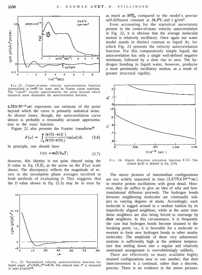
Even accounting for the statistical uncertaintypresent in the center-of-mass velocity autocorrelationin Fig. 22, it is obvious that the average molecularmotion is relatively oscillatory. Once again our watermodel stands in distinct contrast to liquid Ar, forwhich Fig. 23 presents the velocity autocorrelationfunction. For this comparatively simple liquid, theautocorrelation has only a single well-defined negativeminimum, followed by a slow rise to zero. The hy-drogen bonding in liquid water, however, producesa more persistently oscillatory motion, as a result ofgreater structural rigidity.

4.78X1O-13 set represents our estimate of the pointbeyond which the curve is primarily statistical noise.At shorter times, though, the autocorrelation curveshown is probably a reasonably accurate approxima-tion to the exact function.

Figure 22 also presents the Fourier transform4’

F(w) = /d (v(0) -v(O))- (v(O) -v(t) > cos(ot)dt

. (5.6)

In principle, one should have

F(0) =mD/kBT; (5.7)

however, this identity is not quite obeyed using theD value in Eq. (5.3), as the arrow on the F(w) scaleshows. The discrepancy reflects the magnitude of er-rors in the incomplete phase averages involved inboth methods of evaluating D. This suggests thatthe D value shown in Eq. (5.3) may be in error by

1.5

A 1.0

N>

\vr\z=-t. .5zX”

0

-.20 _I 5 .30 45 .60 .75 .90

t*

F I G. 23. Normalized velocity autocorrelation function forliquid argon; p*=O.Sl, T*=O.74. The reduced time t* is measuredin units ~~(vt/e)“~.

0 .436 .a71 1.306 1.742

t ( 10-12 S E C )

F I G. 24. Dipole direction relaxation function T,(l). Therelated $1(t) is defined in Eq. (5.9).

The stereo pictures of intermediate configurationsare too widely separated in time (2.177.5)<10-13 set)to resolve proton oscillations with great detail. How-ever, they do suffice to give an idea of why and howtranslational diffusion proceeds. The hydrogen bondsbetween neighboring molecules are continually sub-ject to varying degrees of strain. Accordingly, eachmolecule is tugged around in a random fashion by itsimperfectly aligned neighbors, while at the same timethose neighbors are also being forced to rearrange byfhei~ neighbors. In this circumstance, it is frequentlythe case that hydrogen bonds become strained to thebreaking point; i.e., it is favorable for a molecule toreorient to form new hydrogen bonds to other nearbymolecules. The amplitude of these very anharmonicmotions is sufficiently high at the ambient tempera-ture that settling down into a regular and relativelyunstrained arrangement is overwhelmingly unlikely.

There are effectively so many available highlystrained configurations near to one another, that theirinterconversion is a continual, rather than a discrete,process. There is no evidence in the stereo pictures

M O L E C U L A R D Y N A M I C S S T U D Y O F L I Q U I D W A T E R 3351

for a hopping process between alternative positionsof mechanical stability. Instead, translational diffu-sion proceeds via individual molecule participation inthe continual restructuring of the labile random hy-drogen-bond network.

B. Dipole Direction Relaxation

The forces of hydrogen bonding between moleculesprevent rapid turning over of those molecules. Theautocorrelation function for the dipole direction of agiven molecule

rl(l) = (l@)(O) ‘p+(r)(t) >= (P1[cosej(l)]) (5.8)

clearly shows this rotational retardation. It is plottedin Fig. 24 both in direct form, as well as logarith-mically in terms of the quantity

$1(t) = - (103At/lt) ln(Pr[cosej(t)]). (5.9)

After a brief period of initial libration lasting roughlylo-r3 set, a long monotonic decay ensues which ap-parently persists well beyond the time limit imposedby the computation. By fitting a simple exponentialfunction to I’1 in the monotonic range, one infers alongest relaxation time 71 equal to about 5.6X lo-r2 sec.

It has been claimed48~4g that the macroscopic dielec-tric relasation time (for polar liquids with large co)should be $ or 2 times as large as rl. Our calculationswould then imply for water at 34.3”C:

8.4X10-r2 set _<7d<11.2X10-12 sec. (5.10)

The measured dielectric relaxation time at this tem-perature is50

ra=6.7X 1O-*2 set, (5.11)

so taking the various imprecisions into account, ourwater model seems not to be too far out of line.

0 .436 ,871 1.306 1.7,

t ( lO-'2 SEC )

FIG. 25. Relaxation function I’*(t) for the dipole directionsecond harmonic. The related function &(t) is defined in Eq.(5.14).

The autocorrelation function I’r(t) may be regardedas the leading member of an infinite sequence ofautocorrelation functions for spherical harmonics ofascending order:

rZ(t) = (PL[Pj”‘(O) ‘Q)(t)]), (5.12)

where PE is the Zth Legendre polynomial. If the unitdipole direction vector pi(l) moved in time by a truerotational Brownian motion, the rr would decay ex-ponentially with relaxation times rr all simply relatedto 71:

r2=271/1(lfl). (5.13)

In order partially to test this possibility, r2(t) wasevaluated for the present water model, along withthe Z=2 analog of $.J,:

&(t)=-(103At/t) lnrz(l). (5.14)

These two functions are plotted in Fig. 25. Again aninitial rapid libration shows up, followed by a longermonotonic decay. This monotonic portion is certainlynot precisely characteristic of a single exponentialdecay, but indicates that the most persistent com-ponent exhibits a relaxation time

r2S2.1X 10-r* sec.

The ratio of I= 1 to I= 2 relaxationwater model computation is thereforethan the ideal Brownian motion ratio

(5.15)

times for thesomewhat less3:

(5.16)

This diminution should be espected however, sincethe water molecule rotational motion corresponds moreclosely to a sequence of finite stochastic jumps, ratherthan to the infinitely rapid infinitesimal jumps im-plied by classical Brownian motion (Wiener processsr) .

The nuclear magnetic resonance spin-lattice relaxa-tion time T1 contains a contribution, due to molecularrotation, that in principle measures r2(t) if the rota-tion is isotropic.52 Krynicki53 has inferred from his T1measurements how 72 should vary with temperature;his results imply that

7221.9x 10-l* sec. (5.17)

In view of the several uncertainties involved in inter-pretation of the experiments, the r2 values (5.15)and (5.17) are in satisfactory agreement.

C. Dielectric Relaxation

The autocorrelation lYl(l) is central to the fre-quency dependence of the liquid’s dielectric constant.We have already noted (Sec. IV. C) that ignoranceof the correct liquid-phase molecular dipole momentlimits one’s ability to predict the static dielectric con-stant co. This ignorance naturally hinders full under-standing of (F(W) as well, as does the present lack

-

3352 A . R A H M A N AND E’. H . S T I L L I N G E R

0 .I .2 .3 .4 .5 .6 .7 .8 9 1.0

E

F I G. 26. Cole-Cole plots for the frequency-dependent di-electric constant e(w). The curves are based upon the Nee-Zwanzig theory, Ref. 49. The reduced coordinates are definedby Eq. (5.19), and c depned by Eq. (5.20). Marks on the curvesindicate frequency in units 1W2 set-I.

of a fully general theory of time-dependent dielectricresponse in polar fluids.

Nevertheless, the recent approximate analysis ofdielectric relaxation by Nee and Zwanzig4g providesa convenient tentative basis on which to convert ourmolecular dynamics results into traditional Cole-Coleplots. 54 They derive the following relation:

EOCE(W) -4 P(W) +4=-

E(W) (eo-6.Y) (2eof%o) /

- & exp(iwt) drl(o .

0 dt ’

(5.18)

for present purposes the high-frequency dielectric con-stant E, corresponds to about the lo-cm+ wavelengthregion, which has been reportes5 to yield an E, of4.5 for water.

By using the previously evaluated I’l(t) and asimple exponential extrapolation beyond the rangeshown in Fig. 24, it is possible to evaluate t(w) andv(w), the real and imaginary parts of ~(w)/Q:

E(W)/EO=S(W)+G(W), (5.19)

from expression (5.18). The precise value of

c = &/EO (5.20)

for our specific model is unknown, but if real waterat 34.3”C gives a reliable indication, it should beroughly 0.06.

Figure 26 shows the Cole-Cole plots obtained forthe G values 0.05 and 0.15. The curves are ratherclose to the classic semicircular shape for w< 2X 1O-12set-I. However for high frequencies, “curlicues” ap-pear which may be attributed to the rapid initiallibrational motion in ITI(

D. Proton Motion and Neutron Scattering

Owing to the fact that protons are strong incoherentscatterers, cold neutron scattering provides a conven-ient experimental tool for the study of single protonmotions in water. It is therefore important to extractinformation from the molecular dynamics computa-

tion that bears specifically on these motions. Thereare in fact several independent dynamical quantitiesthat deserve attention, beyond the mean-square dis-placement that has already been considered.

The angular velocity autocorrelations about thethree principle axes of the molecule:

&z(O)%(t) >/&X2), (Y=l, 2, 3, (5.21)

illustrate one aspect of proton motion. Figure 27presents these three rapidly decaying functions. Allthree indicate a substantial librational, or oscillatory,character. The rates of libration are in the same orderas the reciprocals of the respective moments of inertia:

12-l> 13-l> 11-l; (5.22)

as the insert in Fig. 27 indicates, axis 1 is perpen-dicular to the molecular plane, axis 2 is in the mo-lecular plane, and axis 3 is the twofold molecularsymmetry axis.

A magnified view of the initial portion of I’l(t)(shown previously in Fig. 24) is also included inFig. 27. Only rotations about axes 1 and 2 affectthe dipole direction pj”’ for molecule j, so it is a com-bination of these two motions which affects I’l. Sincethe librational rates are distinctly different aboutthese two “dipole active” axes, we-see why the com-

FIG. 27. Angular velocity autocorrelation functions. Includedfor comparison (bottom) is the initial behavior of I’t(l), shownearlier in Fig. 24. The principal axis numbering is shown in theinsert.

M O L E C U L A R D Y N A M I C S S T U D Y O F L I Q U I D W A T E R 3353 i

bination in I’1 exhibits the oscillatory character lessvividly than the w, autocorrelations themselves.

The spectral resolutions, or Fourier transforms, ofthe W, autocorrelations are defined thus:

MW =l (!&)

Co h&h&) > cos(nt)dt

. (5.23)They are shown in Fig. 28. The positions of theirrespective maxima and centroids again reflect theordering of librational rates according to the inertialmoments.

The autocorrelation of the total angular velocityfor a given molecule,

MO) *o(l) >/(I Q.J 1% (5.24)

may be obtained from a linear combination of theseparate normalized autocorrelations (5.21)) usingweights that follow from the thermal equilibriumconditions,

(w,~) = kBT/I,. (5.25)

The resulting spectrum, jt0t(!2), that follows from(5.24) is presented in Fig. 29.

If the vector @ denotes the position of a givenproton relative to the center of mass of the moleculecontaining it, then the velocity of that proton mea-sured relative to the center of mass will be

0 x e, (5.26)

where o is that molecule’s angular velocity. Sinceour water model molecules are completely rigid, the

I

.4- I49 meV

FIG. 28. Frequency spectra of the angular velocity autocorrela-tion functions.

OI0

i4 8 12 16 2 0 2 4 26 3 2

0. ( lOI S E C - ’ )I

FIG. 29. Frequency spectrum of the total angular momentumautocorrelation function.

length 1 e ( remains fixed so that the proton seemsto be moving on a spherical surface when viewedfrom the center of mass. The appropriate normalizedvelocity autocorrelation function for description ofproton diffusion on the sphere is the following:

4(t) = K@(O) xQ(0)l*re(o X~(~)lV~l @X@ 1%(5.27)

and we shall represent its spectral resolution in theusual way:

cp(O) = r+(t) cos(Ot)dt. (5.28)0

The Fourier transform % may be related to thetime dependence of the mean square of u, the protondisplacement relative to the center of mass. Specifi-cally, it is easy to establish that

(I u(t) p>= (;) (I @XW lz)/.(l-c~(at))~(Q)~.0

.

(5.29) +

Since the spherical surface upon which the protonmust move is bounded, this last quantity must ap-proach a finite limit as t-+m. Hence a(O) mustvanish, and the integral

J-W%(n)dn (5.30)

0

is constrained to a value set by simple geometricalconsiderations.

The functions 4(t) and a(Q) obtained from themolecular dynamics are shown in Fig. 30. The formerdemonstrates once again the substantial oscillatorycomponent of proton motion. To evaluate @(Q) nu-merically from 4(t), an integration cutoff time hadto be imposed, which is indicated in Fig. 30 by anarrow. The resulting numerical %(Q) fails to vanishat the origin, due to absence of a long time negativetail in 4(t) that is associated with the eventual (=:5X

3354 A . R A H M A N ;\SD 1:. H . S T I L L I N G E R

8 12 16 20 24 28 32

-:;0 2

t (lO-‘3sec)

FIG. 30. Normalized velocity autocorrelation function (andits frequency spectrum) for proton motion relative to the centerof mass.

10-12 set) turning over of molecules, The dashed curveshown for 9 near the origin represents our estimateof how the accurate @ (incorporating the effect ofthe negative $J tail) would have to behave, includingthe fact that integral (5.30) is fixed.

The central quantity probed by neutron inelasticscattering from water is the Van Hove5’j self-correla-tion function Ga(r, t) for protons. This function givesthe spatial distribution at time t (in an ensemble ofidentically prepared systems) for a proton initially atthe measurement origin when t=O. Its spatial Fouriertransform in the classical limit is given by

17s(k, t) = (exp{zk.[r(t)-r(O)]) >. (5.31)

A substantial body of theoretical effort has beendevoted to understanding these self-correlation func-tions in general liquids. A particularly popular ap-proach, the “Gaussian approximation,“57 has beenmotivated by the nature of the macroscopic diffusionprocess. This approximation requires Gs(r, t) to be aGaussian function in r at all times, with a widthchosen to reproduce the correct microscopic mean-square displacement (I r(t) 1”). The equivalent requir-ement is that F,(K, t) have the form

F,(K, t) =exp[-QK2(r2(t))]. (5.32)

Our molecular dynamics calculation enables us totest the validity of Eq. (5.32) directly, since inde-pendent calculations of (r”(t) ) and of expression (5.31)are possible. Figure 31 graphically shows the test ofEq. (5.32) for three wave vector choices that areconsistent with the periodicity cube employed in thedynamics

Ka=9.517, 14.276, 19.034. (5.33)

Although the specific Gaussian approximation (5.32)accounts qualitatively for the behavior of F,(k, t), it

is obvious that substantial quantitative errors arise.For each wave vector, the Gaussian F,(k, t) decaystoo rapidly to zero with increasing t in Fig. 31. If onewere to force neutron scattering measurements to fitexpression (5.32) in this k range, the apparent (r”(t) )would increase too slowly with t; i.e., the apparentself-diffusion constant would be anomalously small.

The failure of approximation (5.32) for intermediateK values is connected to the fact that the Van Hovefunction Gs(r, t) is not itself Gaussian in r for inter-mediate times.58 It is worth recalling that a distinctlynon-Gaussian Gs(r, t) has also been found in moleculardynamics calculations on liquid argon.n

The fact that the actual F,(k, t) curves in Fig. 31decay in time more slowly than their Gaussian analogsis related to the narrowing that has been observedin water for neutron quasielastic scattering peaks.5g*60One conceivable way in which this narrowing couldbe explained would be a jump diffusion mechanism,whereby molecules would execute occasional hops ofconsiderable length between quasicrystalline sites ofoscillation in the liquid. Indeed theories of preciselythis character have been advanced to explain theneutron e.xperiments by Singwi and Sj61ander,61 andChudley and Elliot.62 The former authors concludefor example that at 20°C each water molecule oscil-lates in place for about 4X 10-12 set before experiencingrapid diffusion (a “jump”) to a new position ofoscillation.

In confronting a phenomenon as complicated asproton motion in liquid water must surely be, oneruns the risk that experimental data such as neutronscattering can be ercplained in a variety of ways.Thus, it may be that a jump diffusion mechanism is

FIG. 31. Spatial Fourier transform F$(k, t) of the Van Hoveself-correlation function for protons. Curves for the three valuesku=9.517, 14.276, 19.034 are shown. In the lower graph, theGaussian approximation (5.32) gives the lower curve for eachpair. In the upper logarithmic plot, the Gaussian approximatroncurves are coincident ( (+)/6u).

M O L E C U L A R D Y N A M I C S S T U D Y O F L I Q U I D W A T E R 3355

suficie~lt to esplain that data, but not logically neces-sary. In fact, the jump diffusion mechanism definitelyconflicts with our molecular dynamics results. Boththe temporal correlations, and the sequence of stereopictures, show that well-defined quasicrystalline sitesof residence do not exist in liquid water. The diffusivemolecular motions are much more continuous andcooperative and apparently depend strongly upon thedistinctive liquid-phase random hydrogen-bond net-work that is present and forever transforming itstopological character.

Sakamoto et ~1.~~ have computed proton mean-square displacements vs time by Fourier-transformingneutron scattering data. Although their results havebeen interpreted as further support for the jump dif-fusion mechanismG4 such an interpretation is subjectto esnctly the same uniqueness criticism. For thediffusion times probed by the analysis of Sakamotoet al. (2 X lo-l3 to lo-r1 set) , the mean-square protondisplacements are similar to those shown in Fig. 21for the molecular dynamics. In this time range, theonly clear distinctive feature exhibited by both ap-proaches is that the proton displacement curve liesabove the straight line passing through the origin withslope corresponding to the correct D. In order toeffect a discriminating experimental test of diffusionmechanisms in liquid water, sufficient improvementin experimental technique is required to examine timesof the order of lo-l4 set accurately.

As a final aspect of water molecule kinetics, wemention that the velocity autocorrelation for protons(within present accuracy) is found to be the sum ofthe molecular center-of-mass autocorrelation (Fig. 22))and the “motion on the sphere” autocorrelation (Fig.30). Thus the translational and rotational motions ofthe molecules seem to proceed independently of oneanother, on the average. Figure 32 therefore exhibitsthe total proton motion spectrum that was obtained

4 12 16 20 24

F I G. 32. Frequency spectrum for proton total velocity auto-correlation function. As the legend indicates, this was obtainedas a linear combination of the spectra in Figs. 22 and 30.

by linear combination of the spectra reported in Figs.22 and 30.

VI. TEMPERATURE VARIATIONS

In addition to the one temperature studied atlength in this paper, 34.3”C, our water model needsand deserves to be examined at several other tem-peratures to allow instructive comparisons to be car-ried out. These extensions are, in fact, underway andwill be reported in due course. For the present, weshall only briefly mention a low temperature run toadd perhaps some more credibility to our water model.

This new run involved the same condition as itspredecessor (#=216, 18.62 8 cubical box with peri-odic boundary conditions), but the temperature wasonly 26S’K (--8.2”C). The system therefore corre-sponded to liquid water in a state of moderate super-cooling, but under the circumstances that prevail,essentially no chance existed for the liquid to nucleateand freeze into ice. The run lasted 4000 A1.

The osygen-nucleus pair correlation function goo(*) (Y)computed for this lower temperature superficially re-sembles the one shown in Fig. 3. It approaches unitywith increasing Y rapidly enough again to excludebulky “clusters” or “icebergs” from serious considera-tion. Furthermore, the distance ratio for second andfirst peaks is rather close to the ideal value for tetra-hedral hydrogen bonding. However, the first maximumof goo(*)(y) is significantly larger (2.97, compared to2.56 in Fig. 3) and the succeeding minimum deeper.The second maximum appears to be better developedand narrower. Evidently the random hydrogen-bondnetwork has tightened up considerably, by discrimi-nating against severe distortions of the ideal tetra-hedral coordination geometry.

The stereo pictures that have been produced fromthis lower temperature run bear out that conclusion.The hydrogen bonds that form between neighboringmolecules appear to be more nearly linear and toobserve the tetrahedral angles of approach more fre-quently. Although the bonds in the random networktend to strengthen at lower temperature, this doesnot imply that it is easier then to identify a few“interstitial” molecules; as before we see no clearexamples of any interstitials. Also, the liquid seemsto show no marked tendency anywhere to organizethe beginnings of ice nuclei.

To the extent that x-ray scattering experimentspredominately reflect gooo) (r) , our structural shiftswith temperature variation agree qualitatively withmeasurements reported by Narten, Danford, andLevy.2g

Naturally the strengthening of the interactionstends to slow down molecular diffusive motions mark-edly. The self-diffusion constant D at 265°K is foundto be approximately 1.5X1O-5 cmz/sec for the mo-lecular dynamics simulation. Once again this seemsto be rather larger than the experimental value 0.7.5f

i

c

33.56 A . R A H M A N A N D F . H . S T I L L I N G E R

0.03 X 1w5 cm2/sec, 65 but comparison of the ratio ofvalues at -8.2 and 34.3’C (0.36 theoretical, 0.26 ex-perimental) indicates roughly the necessary rapid tem-perature variation for D. Furthermore, the simpleenergy resealing discussed in the following sectioninduces far better agreement with the measured Dvalues at both resealed molecular dynamics tem-peratures.

In order to round out the study of temperaturevariations, we intend to study our model up to theneighborhood of the critical temperature (374OC).This should provide a comprehensive account of thethermal disruption .of the hydrogen-bond network,and should permit a reasonably accurate evaluationof the constant volume heat capacity.

VII. DISCUSSION

In order to continue systematically applying themolecular dynamics method to water, two types ofextensions of the present work are necessary. Thefirst involves expanding the domain of application ofthe model employed here to include a wide range ofdensities and of temperatures (mentioned in the pre-ceding section), as well as to include solvation andinterface studies. The second type of extension is theanalysis of ways in which the effective pair inter-action V&2) should be modified to yield a more ac-curate description of real water. These two aspectsneed to be carried forward in parallel, since accuratedetermination of the properties implied by a givenHamiltonian, in comparison with experimental results,provides the basis for modification.

With respect to future study of aqueous solutions,it should be mentioned that the model employed inthis paper can be immediately adapted to simulationof a particularly simple solute. By retaining only VW[see Eq. (2.5)] in the effective pair interaction be-tween a chosen molecule and all the others, thatmolecule should reasonably well behave as a neon atomif in addition the full mass were placed at its center.This single solute particle of course could not hydro-gen bond to its neighbors. One would then be par-ticularly interested to see if the surrounding watermolecules organized themselves into a sort of “cage”analogous to those present in clathrates. The resultswould be especially interesting in view of the “hydro-phobic bond” concept that has been proposed to ex-plain the interaction of nonpolar solutes in water.@js’jr

In order to broaden the scope of solution studiesto include other solutes, information will be requiredabout the interaction of water molecules with a va-riety of ions and molecules. Extensive quantummechanical calculations would have considerable valuein determining characteristic shapes of potential sur-faces for water molecules in interaction with distinctchemical groupings, e.g., methyl groups, carbonyl

groups, hydroxyls, conjugated double bonds betweencarbon atoms, amines, etc. With such information inhand, it would become possible to design moleculardynamics calculations to study the hydration of bio-logical macromolecules and the interaction of waterwith membranes.

The simplest of all possible modifications that mightbe applied to the effective potential would be thestrength resealing mentioned briefly at the end ofSec. III. If one were to choose the interaction energy(VN)/~ and the self-diffusion constant D as havingcentral importance, then a resealing factor

l+p= 1.06 (7.1)

would have the effect of changing the temperatureto 52.8”C, while inducing much better agreement thanpreviously between calculations and experiment bothfor mean interaction energy:

( VN)/IV= - 9.735 kcal/mole (molecular dynamicsresealed) ,

= -9.63 kcal/mole (exptl, 52.8”C), (7.2)

and for the self-diffusion constant:

D = 4.3X 1O-5 cm2/sec (molecular dynamics resealed) ,

=4.1X10-+ cm2/sec (exptl, 52.8”C). (7.3)

At the same time, of c e the rotational relaxationtimes rr and TZ would by (l+{)‘/‘, makingthem apparently agree with experiment. Butsince the theoretical f s are weak in whichrl and r2 ar ated to dielectric and NMR experi-ments, this greement should probably be givenrelatively little weight at present.

Energy resealing also affects the value predicted bymolecular dynamics for the Kirkwood orientationalcorrelation factor. When the measured EO for waterat 52.8’C is inserted in Eq. (4.17) to convert GKto gK, one obtains

gk = 2.72, (7.4)

somewhat smaller than the “unscaled” result 2.96 inEq. (4.19). The previously cited work of Harris,Haycock, and Alder,34 which suggests gK should bein the range 2.5-2.6 at this temperature, also sup-ports the resealing.

The same energy resealing factor 1.06 seems tenta-tively also to produce considerable improvement inagreement with experiment for the low temperaturerun mentioned in the preceding Section. Although thenominal temperature 26YK (-8.2”C) for that runcorresponded to supercooled water, the resealed tem-perature 280.9”K (7.7’C) lies above the melting pointof ice. Eventually, it would be very interesting tocarry out a molecular dynamics simulation on a

M O L E C U L A R D Y N A M I C S S T U D Y O F L I Q U I D W A T E R 33.57

strongly supercooled water sample (even on the re-scaled basis), to see what type of local order arises.

Beside the strength resealing for V,J2), a lengthresealing is also possible. This would produce a shiftin density (rather than temperature) and would re-quire reinterpretation of all quantities dependent uponthe length unit. At present no compelling evidencemotivates such a distance resealing.

Probably the principal criticism which might bedirected toward our choice for VeJ2) is that it issomewhat too “tetrahedral.” However, it is significantto have observed that even in the presence of thistetrahedral bias, the local structure produced in ourmodel “water” still manifests very substantial ran-domness, and fails to mimic known crystal structures.It is therefore quite unlikely that a less tetrahedralV,rr(*), at a given temperature, would be more suc-cessful in building liquid-phase networks akin to theice lattice or the clathrates at the local level.

Barker and Watts@’ have carried out a Monte Carlocalculation for N=64 water molecules (at 25”C),using the RowlinsonGs pair potential. Like our owneffective pair potential, the Rowlinson interaction isbased on a four-point charge complex for each mole-cule. However, the positions of these charges do notlead to a natural tetrahedral arrangement of neigh-bors. As a result, the computed oxygen-nucleus paircorrelation function tends to have a rather largenumber of nearest neighbors (6.4 out to distance3.5 ii), and the positions of first and second maximaare far from the ideal tetrahedral ratio. Although theRowlinson potential may provide a reasonable accountof the interaction for isolated pairs of water moleculesin the vapor, it probably deviates too far from thetetrahedral directionality required of a condensedphase Fen c2) that must lead to essentially universalfourfold coordination in aqueous crystals.

A possible modification of our own V&2), Eq. (2.5),which does not seriously compromise its directionality,would be to shorten the distance from the oxygennucleus to the negative point charges, without chang-ing any angles or the distance to the positive charges.At the same time it would be necessary to adjustthe parameters 7, RL, and Ru, to maintain the strengthand length of undistorted hydrogen bonds. This changewould permit greater freedom in approach directionfor formation of linear hydrogen bonds. The meaninteraction energy in the liquid should thereupon in-crease in magnitude. It must be left for future inves-tigation, however, to determine what the concomitanteffects on static correlation functions and kineticproperties would be.

ACKNOWLEDGMENT

The authors are indebted to Dr. Seymour H. Koenig,IBM Watson Laboratory, for arranging a generous

grant of computer time at the IBM ComputationCenter to carry out the low temperature run reportedbriefly in Sec. VI.

APPENDIX A

Given x; and xj [see Eq. (3.1)] and the positionsof the oxygen and four point charges in each mole-cule, we can calculate the list of 17 distances: rij,the oxygen-oxygen distance; and 16 point charge dis-tances dtiimj. Then V,rr@) gives rise to a force vectorof magnitude:

24(E/r,j)[2(U/rij)12- (U/Yij)6]

--6lI(rij--RL) (RU-yij)l(Ru-R,)3J21c,(X;, xj) (A l )

acting between the two oxygen nuclei. The term withV,I [Eq. (2.8)] is present only for RLjr,j<Ru [seeEq. (2.9)].

Each pair of point charges in the respective mole-cules gives a force vector of magnitude

S(rij) (0.19e)2(--l)Qi+a,/dpiuj (A2)

acting between that pair.The Cartesian components of these forces are ob-

tained simply by multiplying the magnitudes by ratiosof the type (G;-Xoj)/rij and (~~~-z~~)/d_~.

These 17 forces then give, by a summation ofrespective components, the total body force actingon a molecule. Using the transformation matrix whichrotates xyz into x’y’z (Fig. 2), the components of thetorque Nj [Eq. (3.5)] can also be calculated fromthe components of the force acting on each of thefive points of a molecule (the positions of the oxygennucleus and the four point charges). Adding theinertial terms [Eq. (3.6)] gives the derivatives ofthe angular velocities about the principal axes ofinertia.

.

To indicate the scheme’O we have used for solvingthe Newton-Euler equations of motion, we shall takethe following three differential equations as proto-types for Eqs. (3.3), (3.6), and (3.7), respectively,

Wdt=dx, P, 91,dpldt=Wp, 9). (A3)

Here x typifies center of mass Cartesian coordinates,q is the angular velocities about the principal axes ofinertia, and p is the Euler angles.

The problem is to get 2, p, q at t+At knowing thevalues at time t. Assume that the calculation hasalready been initiated so that, apart from 2, p, q at t,we also know the first five derivatives of x and thefirst four of p and 4. Let x,,, e.g., denote

[(At) “n !]d’%/dtn.

3358 A . R A H M A N A N D F . H . S T I L L I N G E R

We predict the values of all these quantities atI+At by using the Pascal triangle:

%‘=%+%+x2+%+s+x5,

x1’=~~+2~2+3~,+4~4+5~5,

x~‘=x2+3~3+6~4+10~5,

x3’= x3+4x4+ 10x5,

x4’= x4+5x5, L44)

and similarly for ~0’. - -p3’ and 40” -43’.Using the predicted values XQ’, pi, qo’ we calculate

f(ro’, PO’>, dxo’, PO’, 40’1, and h(po’, PO’). Denote thesevalues by f, g’, h’.

The differences,

A=[(~)2/2!]f)-zz’,

B= (At)g’-q<,

C= (At) h’-p<, (As)

are then used to correctfollowing way:

x,(t+ At) =~n’+fnzA

pm(t+At) =pm’+fd

qm (l+ At) = qm’+f& twhere

the predicted values in the

(?z=O, 1, **-, S),

(m=O, 1, * * *, 4), (A6)

fm=W, fa=251/360, fz= 1 ,

f==ll/lS, fa=1/6, f52=1/60, ( A 7 )and

f01=251/720, fll=l, f21=11/12,

f31= l/3, fa = l/24. (A@

It will be seen from Ref. 70 that these coefficientsdepend on the “order” of the procedure used. In ourmolecular dynamics runs on water we have used afifth-order procedure for the center-of-mass motionand a fourth-order one for angular motion.

At the start of the calculation the most convenientprocedure is to take all the derivatives equal to zero.In the case of interest here (Newton-Euler equa-tions) , the angular velocities (typified by q in t h eschematic presentation) can also be equated to zeroat the start of the calculation. The “aging” of therun then necessarily leads to a solution effectivelyunrelated to the specific starting procedure.

APPENDIX B

In the convention utilized for the molecular dy-namics calculations, each molecule experiences forcesand torques due only to those other molecules withina cutoff radius R. In the presence of a uniform, weak,external electric field Eext, the system will developa uniform polarization P. Classical electrostatics re-

quires4xP= (e-l)E, (Bf)

where the electric field E is composed both of theimposed field Emt, and the internal field Eint due tothe nonvanishing polarization

E=Em+,+Ei,t. (B2)

The contribution of polarization in a small volumeelement 6v at position r’, to the internal field at posi-tion r, is the following:

-V,[GvP(r’)].V+(I r -r ’ 1-l). (B3)

In writing an expression for the polarization P(r) formolecules at r, that is consistent with the moleculardynamics, we clearly must integrate quantity (B3)only over the sphere of radius R surrounding posi-tion r:

47rP(r) = (co-l)[Eert

-/ _

,Fr,,<R dr’V,P(r’) . V,J (1 r-r’ I-9 I- W

The integral may easily be evaluated to yield:

4xP= (e,- 1) [Eext- (47d3P1, WIor

P=[3(~-1)/4?r(~a+2)]E,,t. (B6)

Not surprisingly, relation (B6) is exactly the sameone that applies to the polarization of a sphericaldielectric sample with a real boundary surface, placedin ‘a vacuum region initially containing E,t only. Wemay therefore call upon the Kirkwood theory of polardielectrics,3o which applies to those spherical specimenconditions.

Irrespective of boundary conditions, the polariza-tion consists of a part P, due to induced molecularmoments, plus a part due to reorientations that isproportional to (M2), the mean-square system momentin the absence of external fields’r:

P = P,+ (P/3 V) (M?E,t, (B7)where V stands for the system volume. The importof expressions (B6) and (B7) taken together is thatfor a given co, the quantity (M2)/V should be thesame for the molecular dynamics situation as it isfor a spherical dielectric sample in a vacuum.

Kirkwood has shown that the local moment m ofa fixed molecule and its immediate surroundings, in adielectric sphere, is related to the average moment Mof that sphere by

M=[%/(Q+~) (2~0fl)bn. (B8)

It is precisely the distinction between these twomoments which & and gx for the dielectric spherereflects, so we must have

GK=[%/(m+2) &0+1)1g~. (B9)

In view of the equivalence of the dielectric sphere to