Indian Institute of Pulses ResearchKanpur - 208 024

Easy & rapid

Reproducible genotyping

Accurate phenotyping

Authentic mapping population

Choice of parents

Molecular Markers in Crop Improvement

Molecular Markers in Crop Improvement

Agr search with a uman touchAgr search with a uman touch

gj dne] gj Mxjfdlkuksa dk gelQjHkkjrh; d`f"k vuqla/kku ifj"kn

ICARHkkd`vuqi

Hkknvl

F PO U LE ST EU STI RT ES SNI E

AN

RAI CD HNI

Molecular Markers inCrop Improvement

D. DattaSanjeev Gupta

S.K. ChaturvediN. Nadarajan

Indian Institute of Pulses ResearchKanpur - 208 024

ICAR

Printed : September, 2011

Published by : Dr. N. Nadarajan, DirectorIndian Institute of Pulses Research, Kanpur

Edited by : Mr. Diwakar Upadhyaya

Printed by : Army Printing Press, 33, Nehru Road, Sadar Cantt, Lucknow Tel: 0522-2481164

Correct citation : Datta, D., Gupta, Sanjeev, Chaturvedi, S.K. and Nadarajan, N. (2011):Molecular Markers in Crop Improvement. Indian Institute of Pulses Research,Kanpur - 208 024

Preface

With the advent of marker-assisted selection (MAS), a new breedingtool is available to make more accurate and useful selections in breedingpopulations. MAS allows heritable traits to be linked to the DNA segments thatare responsible for controlling that trait. These segments of DNA or QTLs(Quantitative Trait Loci) can be detected through specific laboratory techniques.

The most commonly used method is Polymerase Chain Reaction (PCR)that amplify segments of DNA linked to heritable traits such as yield or diseaseresistance. This method is useful because the DNA that we amplify is different(polymorphic) between cultivars. It is this difference that we use to determinewhether the plant has the desired trait or not. The process in which thedifferential DNA sites (or primer sites) are explored, comes from genetic mappingtechniques, i.e. RAPD, microsatellites etc. With a marker assisted selectionbreeding program the simpler methods are necessary since they are time andcost effective. PCR is an effective method for generating large quantities of aspecific DNA sequence from a small amount of starting DNA. This techniqueis useful for a MAS breeding program because the results are reliable.

To learn how MAS works, basic molecular biology principles need to beunderstood. The present bulletin “Molecular markers in crop improvement”has been designed to provide a basic understanding with regards to use ofmolecular markers in crop improvement. This bulletin describes basic conceptsused in marker assisted breeding programme, different applications of MASand basic principles underlying DNA extraction, PCR, running of gel and dataanalysis. The help rendered by Shri Diwakar Upadhyaya in editing the manuscriptis duly acknowledged. We hope that this bulletin will be of immence use forstudents and trainees of molecular breeding.

Authors

Contents

Preface

1. Basic Concepts 1

2. Use of Molecular Markers in Breeding Programmes 24

3. Principles of Basic Techniques 34

4. Literature Cited 49

1

Basic Concepts

During the past 20 years there has been rapid growth in the relatively new field of plantbiotechnology and its associated techniques. These have application, not only for the manipulationof biological systems for the benefit of mankind, but also to undertake studies for better understandingof the fundamental life processes. Consequently, it has become the fastest and most rapidly growingtechnology in the world. Biotechnology is defined as “any technique that uses living organisms(or parts of organisms) to make/ modify products, to improve plants and animals or to developmicroorganisms for specific uses”. It offers efficient and cost-effective means to produce anarray of novel, value-added products and tools. It has the potential to increase food productivity,reduce the dependency of agriculture on chemicals, lower the cost of raw materials and reduce thenegative environmental impacts associated with traditional production methods.

Conventional breeding is a dynamic area of applied science. It relies on genetic variation anduses selection to gradually improve plants for traits and characteristics that are of interest for thegrower and the consumer. Another important way of improvement is the introduction of new geneticmaterial (e.g., genes for biotic and abiotic stress resistance) from other sources, such as gene bankaccessions and related plant species. Although, current breeding practices have been very successfulin producing a continuous range of improved varieties, recent developments in the field of molecularbiology can be employed to enhance plant breeding efforts and to speed up cultivar development.Modern biotechnology provides new tools that can facilitate development of improved plant breedingmethods and augment our knowledge of plant genetics. The discovery of restriction enzymes bySmith and Wilcox, and the polymerase chain reaction (PCR) by Kerry Mullis and his group hascreated opportunity to understand the composition of organisms at the DNA level, and obtain a so-called genetic fingerprint. These studies are routinely done by the separation of DNA-fragments ona gel that results from a selective digestion of DNA with enzymes or from a selective amplificationof DNA using PCR. DNA fragments that result in different gel patterns between samples orindividuals are called polymorphic markers. The visible differences on the gel result from differencesat the DNA level. Not all types of markers are the same; the information content depends on themethod that is used to obtain the marker data and the population in which the markers were‘scored’. Advanced tools for the retrieval of marker data and the subsequent analysis have beendeveloped that allow quick and reliable results in most plant species.

Molecular (DNA) markers are segments of DNA that can be detected through specificlaboratory techniques. For detection of markers, either restriction enzymes or Polymerase ChainReaction (PCR) or their combination are used to generate/amplify the DNA sequences that arelinked to a heritable trait such as yield or disease resistance. With the advent of marker-assistedselection (MAS), a new breeding tool is now available to make more accurate and useful selectionsin breeding populations. The objective of this section is to introduce genetic terminologies andconcepts associated with molecular markers.

2

Allele

One alternative form of a given allelic pair - tall and dwarf are the alleles for the height of apea plant. More than two alleles can exist for any specific gene, but only two of them will be foundwithin any diploid individual. In terms of molecular marker the variant of a DNA sequence isreferred as an allele. An allele defined by molecular means should have exactly the same geneticproperties as a phenotypically defined allele. Molecular alleles should segregate by the same Mendelianprinciples as phenotypic alleles. Mostly, molecular alleles are selectively neutral. Theories of populationgenetics apply to molecular alleles as well.

Backcross

It is the cross of an F1 hybrid to any one of the homozygous parents.

Testcross

It is the cross of any individual to a homozygous recessive parent. It is used to determine ifthe individual is homozygous dominant or heterozygous.

Pure line

An individual that breeds true to type for a particular trait. This was an important innovationbecause any non-pure (heterozygous parents) would confuse the segregation ratio in geneticexperiments.

Homozygote

An individual which contains only one allele at the allelic pair, for example ‘TT’ is homozygousdominant and ‘tt’ is homozygous recessive. Pure lines are homozygous for the gene of interest.

Heterozygote

An individual which contains one of each member of the gene pair, for example the ‘Tt’heterozygote.

Dominance

It is the ability of one allele to express its phenotype at the expense of an alternate allele. Itrepresents the major form of interaction between alleles.

3

Epistasis

The interaction between two or more genes to control a single phenotype. Epistasis is theinteraction between different genes. If one allele or allelic pair masks the expression of an allele atthe second gene, that allele or allelic pair is epistatic to the second gene.

Suppressor

A genetic factor that prevents the expression of alleles at a second locus. This is an exampleof epistatic interaction.

Modifier genes

Genes that have small quantitative effects on the level of expression of another gene. Insteadof masking the effects of another gene, a gene can modify the expression of a second gene.

Genotype

In general, genotype is the genetic architecture of an individual. Genotype is also used torefer to the pair of alleles present at a single locus. For a diploid organism, with alleles ‘A’ and ‘a’three possible genotypes are AA, Aa and aa. The expression of the genotype is affected by thegenetic constitution of the individual and the environment. With reference to molecular markers,genotype is used to refer to the alternate DNA sequences (molecular alleles) of an individual.

Phenotype

In classical terms phenotype is anydetectable characteristic of an organismdetermined by G + E + G × E interactionsand inherited as Mendelian factor.Phenotype is used to describe a trait/morphology of an individual viz., flowercolour, whereas phenotypic value is themean of the measurements of a trait viz.,height of a plant, weight of a fruit.

Fig. 1: Wild pigeonpea sowing leaf and pod phenotypes

4

PhenotypingThe term ‘phenotyping’ of mapping population refers to scoring (disease resistance, yield or

any other morphological observation) of individuals of the mapping population.

GenotypingIt is a rather loose terminology to describe the DNA profiling (RFLP, RAPD or PCR profiles)

of individuals of the mapping population or the breeding population for detecting presence/absenceof molecular markers. Thus, genotyping is done to generate information on the status of individualswith respect to presence or absence of a set of specific molecular markers.

Genetic markerAny easily scoreable phenotype that is linked with a trait of interest intended to be marked.

They are used to ‘flag’ the position of a particular allele or the inheritance of a particular character.Phenotypes for which the variation observed in the population of interest is partially or entirelyexplained by a single “Mendelian” factor. Three properties that define a genetic marker are: It should be locus-specific It should be polymorphic in the studied population It should be easily phenotyped.The quality of a genetic marker is typically measured by its: Heterozygosity in the population of interest Polymorphism Information Content (PIC).

Polymorphism Information Content is defined as the probability of identifying one homologueof a given parent that transmitted an allele to a given offspring, the other parent being genotyped aswell.

PIC= probability that the parent is heterozygous x probability that the offspring is informative

n

1ij

2j

2i

n

1i

n

1i

2i p2pp1PIC

Morphological markerA morphological marker is expressed as a specific and distinct morphological trait.

Morphological marker may be affected by environment. Generally it is incompletely linked with thegene of interest. Its phenotypic expression may be dependent on growth stage. These markers arerare in a natural population and show extremely low level of polymorphism.

5

Molecular markersMolecular markers are specific fragments of DNA that can be identified within the whole

genome. Molecular markers are found at specific locations of the genome. They are used to ‘flag’the position of a particular gene or the inheritance of a particular character. Molecular markers arephenotypically neutral.

Marker categories

Depending on the technique used for detection and amplification of markers there can bedifferent classes of markers. Restriction fragment length polymorphism (RFLP) is based onrestriction site changes in the target DNA and subsequent hybridization with probe DNA. Randomamplified polymorphic DNA (RAPD), Sequence characterized amplified region (SCAR) andSequence tagged sites (STS) are based on mutation at primer annealing site in the target DNA.Cleaved amplified polymorphic sequence (CAPS) and Amplified fragment length polymorphism(AFLP) are based on both restriction site changes and mutation at primer annealing site in thetarget DNA. Additionally, there are Simple sequence repeat (SSR), Inter simple sequence repeat(ISSR) and Single nucleotide polymorphism (SNP) markers. Highly specialized techniques arerequired to detect SNP’s.

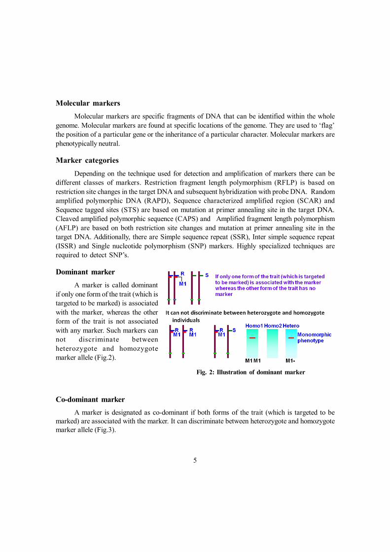
Dominant markerA marker is called dominant

if only one form of the trait (which istargeted to be marked) is associatedwith the marker, whereas the otherform of the trait is not associatedwith any marker. Such markers cannot discriminate betweenheterozygote and homozygotemarker allele (Fig.2).

Fig. 2: Illustration of dominant marker

Co-dominant markerA marker is designated as co-dominant if both forms of the trait (which is targeted to be

marked) are associated with the marker. It can discriminate between heterozygote and homozygotemarker allele (Fig.3).

6

Fig. 3: Illustration of co-dominant marker

Random amplified polymorphic DNA (RAPD)RAPD is a PCR based method, which employs single primers of arbitrary nucleotide sequence

with 10 nucleotides to amplify anonymous PCR fragments from genomic template DNA. In RAPDanalysis, the target sequence(s) (to be amplified) are unknown. In RAPD, PCR is generally carriedout with arbitrary primers. The amplifications are visualized through agarose gel electrophoresis.For amplification to occur it is essential that primers anneal in a particular orientation (such thatthey point towards each other) and the primers must anneal within a reasonable distance to oneanother.

Advantages No prior knowledge of DNA sequences is required

Random distribution throughout the genome

The requirement for small amount of DNA (5-20 g)

Easy and quick to assay

The efficiency to generate a large number of markers

Commercially available decamer primers are applicable to any species

The potential automation of the technique

RAPD bands can often be cloned and sequenced to make SCAR (sequence-characterizedamplified region) markers

Cost effectiveness as compared to other markers.

7

Limitations Dominant nature (heterozygous individuals cannot be separated from dominant homozygous) Sensitivity to changes in reaction conditions, which affects the reproducibility of banding

patterns Co-migrating bands can represent non-homologous loci The scoring of RAPD bands is open to interpretation The results are not easily reproducible between laboratories.

Applications of RAPD Measurements of genetic diversity Genetic structure of populations Germplasm characterisation Verification of genetic identity Genetic mapping Development of markers linked to a trait of interest Cultivar identification Identification of clones (in case of soma-clonal variation) Interspecific hybridization Verification of cultivar and hybrid purity Clarification of parentage

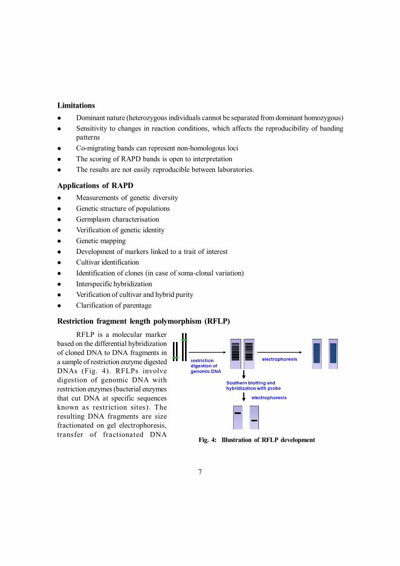
Restriction fragment length polymorphism (RFLP)RFLP is a molecular marker

based on the differential hybridizationof cloned DNA to DNA fragments ina sample of restriction enzyme digestedDNAs (Fig. 4). RFLPs involvedigestion of genomic DNA withrestriction enzymes (bacterial enzymesthat cut DNA at specific sequencesknown as restriction sites). Theresulting DNA fragments are sizefractionated on gel electrophoresis,transfer of fractionated DNA

Fig. 4: Illustration of RFLP development

8

fragments on Nylon membranes (a process known as Southern blotting) and finally hybridizationwith labeled probe to visualize DNA polymorphisms. The first step in RFLP analysis is to derive aset of clones that can be used to identify RFLPs. The two primary sources of these clones forRFLP mapping of plants are cDNA clones and PstI-derived genomic clones. RFLP markers aredefined by a specific enzyme-probe combination. This technique is highly reproducible, and themarkers are co-dominant in their inheritance therefore, allows the differentiation of heterozygotesfrom homozygotes. RFLP procedure is time consuming and expensive but they have been used togenerate saturated genetic map. RFLPs behave like any other Mendelian trait. Each band seen ina Southern blot indicates the presence of one or more restriction sites in a sequence. The sequencecontaining a restriction site is one allele, while the corresponding sequence missing the restrictionsite is the other allele. The “phenotypes” of these alleles are the differences in banding patterns,due to presence or absence of bands. RFLP loci are co-dominant (twice as much informative in agenetic cross as compared to dominant markers like RAPDs).

Amplified fragment length polymorphism (AFLP)

Amplified fragment length polymorphisms (AFLPs) are polymerase chain reaction (PCR)-based markers for rapid screening of genetic diversity. AFLPs are DNA fragments with differentnucleotide sequence of which large number of copies have been amplified via PCR. This techniqueis a combination of the RFLP and PCR techniques. Like RFLP, the AFLPs are highly heritable andpolymorphic. The technique involves restriction digestion of DNA with two different enzymes andligation of two adopters, selective amplification of sets of restriction fragments and gel analysis ofamplified fragments. The amplified products are generally separated on a denaturing polyacrylamidegel and visualized using autoradiography. The technique is more skill demanding than RAPD andalso requires more amount of DNA. The reproducibility of AFLP is ensured by using site specificadopters. AFLP method rapidly generates hundreds of highly replicable markers from DNA of anyorganism, and thus, they allow high resolution genotyping of fingerprinting quality. The time andcost efficiency, replicability and resolution of AFLPs are superior or equal to those of other markers[allozymes,random amplified polymorphic DNA (RAPD), restriction fragment length polymorphism(RFLP), microsatellites], except that AFLP methods primarily generate dominant rather than co-dominant markers. Because of their high replicability and ease of use, AFLP markers have emergedas a major new type of genetic marker with broad application in systematics, pathotyping, populationgenetics, DNA fingerprinting and quantitative trait loci (QTL) mapping.

Cleavage amplification polymorphisms (CAPs)

The scoring of this type of marker is dependent on the variation of size of fragments followingthe digestion of the PCR product by a restriction enzyme. A completely new set of CAPs markerswould be generated from a different restriction enzyme.

9

Simple sequence repeat (SSR) markerMicrosatellite or Simple sequence repeats (SSRs) provide fairly comprehensive genomic

coverage. They are amenable to automation, they have locus identity and they are multi-allelic. Manyagronomic and quality traits show quantitative inheritance and the genes determining these traitshave been quantified using Quantitative trait locus (QTL) tools. SSR markers have wide applicabilityfor genetic analysis in crop improvement strategies. They are widely used in plants because of theirabundance, hyper-variability, and suitability for high throughput analysis.

Inter-simple sequence repeat (ISSR) markerInter-simple sequence repeat (ISSR) are semi-arbitrary markers amplified by PCR in the

presence of one primer complementary to a target microsatellite. Amplification in presence of non-anchored primers also has been called microsatellite-primed PCR, or MP-PCR. Such amplificationdoes not require genome sequence information and leads to multi-locus and highly polymorphicpatterns. Each band corresponds to a DNA sequence delimited by two inverted microsatellites.Like RAPDs, ISSRs markers are quick and easy to handle, but they seem to have the reproducibilityproblem because of the longer length of their primers.

STS and SCAR markersRandom amplified polymorphic DNA (RAPD) is an application of PCR where arbitrarily

chosen 10 base primers are used to search for variation in DNA. RAPD data can contain artifactsand are not fully reproducible. However, RAPDs have been used to generate large number ofgenetic markers useful for linkage mapping quickly and cheaply. RAPD fragments can be separatedon agarose gels. The excised bands from the gel can be re-amplified in to individual bands from gelslices using the original RAPDs primer. The fragments can be cloned and sequenced. The sequencedata can be used to design PCR primers specific to RAPDs fragments, and use PCR to producespecific RAPD’s fragments from genomic DNA, which then can function as sequence taggedsites (STSs) or Sequenced characterized amplified region (SCAR). This method allows for rapidgeneration of STSs derived from RAPD fragments and eliminates the problems associated withreproducibility.

Factors influencing efficiency of a markerEfficiency of markers depends on their closeness to the linked trait; how the phenotype of

marker is affected by environment; consistency in phenotypic expression; how easy is to score thephenotype; and level of polymorphism. Ideally, a marker should be polymorphic, tightly linked withthe trait of interest, highly heritable, co-dominant, easily scoreable and it should not affect thefitness of the individual. DNA markers have many advantages over the morphological markers.DNA markers are phenotypically neutral which is a significant advantage compared to traditional

10

phenotypic markers, highly polymorphic, abundant, usually randomly distributed throughout thegenome, easily scoreable and as such DNA markers are not affected by environment but the geneof interest may be sensitive to GxE and hence its (DNA marker) association with phenotype of thegene may vary with change of environment.

Bulk segregant analysisOften a geneticist is not interested in developing a molecular map, but would rather find a

few markers that are closely linked to a specific trait. Identification of these markers is oftenachieved by a procedure called bulk segregant analysis. The essence of this procedure is thecreation of a bulk sample of DNA for analysis by pooling DNA from individuals with similarphenotypes. For example, you may be interested in finding a molecular locus linked to a diseaseresistance locus. You would create two bulk DNA samples, one containing DNA from plants orlines that are resistant to the disease and a second bulk containing DNA from plants or lines that aresusceptible to the disease. Each of these bulk DNA samples will contain a random sample of all theloci in the genome, except for those that are in the region of the gene upon which the bulkingoccurred. Therefore, any difference in RFLP or RAPD pattern between these two bulks should belinked to the locus upon which the bulk was developed.

PopulationIn classical genetics, population is defined as a group of potentially interbreeding individuals.

Whether haploid or diploid, a population has two basic attributes: gene frequencies and gene pool.Gene (allele) frequency is the proportion of different alleles of a gene in a population, whereas genepool is the sum total of genes in the reproductive gametes of a population. If external forces do notapply then gene frequencies remain unchanged from one generation to the next generation in arandom mating population. It may be noted that gene frequency in particular generation is dependentupon the gene frequencies of previous generation and frequencies of different genotypes dependon gene frequency alone. After one generation of random mating and in the absence of externalforces the genotypic frequencies remain stable which said to be at equilibrium. In terms of molecularbreeding, a population may be defined as a group of individuals originating from a cross combinationthat is capable of representing frequencies of alternate alleles and which allow to calculate genefrequencies in a predictable manner.

Mapping populationMapping population consists of individuals of one species, or in some cases they are derived

from crosses among related species. It is a group of individuals on which genetic analysis is carriedout. It can be either segregating for traits under study or a set of near homozygous lines representinga F2 variation. In both situations mapping population is generally derived from a single cross whoseparents were polymorphic for the trait of interest.

11

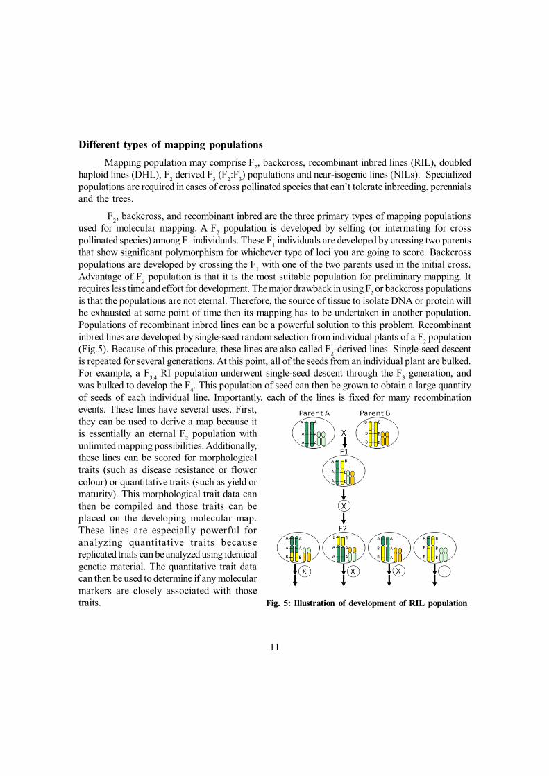
Different types of mapping populationsMapping population may comprise F2, backcross, recombinant inbred lines (RIL), doubled

haploid lines (DHL), F2 derived F3 (F2:F3) populations and near-isogenic lines (NILs). Specializedpopulations are required in cases of cross pollinated species that can’t tolerate inbreeding, perennialsand the trees.

F2, backcross, and recombinant inbred are the three primary types of mapping populationsused for molecular mapping. A F2 population is developed by selfing (or intermating for crosspollinated species) among F1 individuals. These F1 individuals are developed by crossing two parentsthat show significant polymorphism for whichever type of loci you are going to score. Backcrosspopulations are developed by crossing the F1 with one of the two parents used in the initial cross.Advantage of F2 population is that it is the most suitable population for preliminary mapping. Itrequires less time and effort for development. The major drawback in using F2 or backcross populationsis that the populations are not eternal. Therefore, the source of tissue to isolate DNA or protein willbe exhausted at some point of time then its mapping has to be undertaken in another population.Populations of recombinant inbred lines can be a powerful solution to this problem. Recombinantinbred lines are developed by single-seed random selection from individual plants of a F2 population(Fig.5). Because of this procedure, these lines are also called F2-derived lines. Single-seed descentis repeated for several generations. At this point, all of the seeds from an individual plant are bulked.For example, a F3:4 RI population underwent single-seed descent through the F3 generation, andwas bulked to develop the F4. This population of seed can then be grown to obtain a large quantityof seeds of each individual line. Importantly, each of the lines is fixed for many recombinationevents. These lines have several uses. First,they can be used to derive a map because itis essentially an eternal F2 population withunlimited mapping possibilities. Additionally,these lines can be scored for morphologicaltraits (such as disease resistance or flowercolour) or quantitative traits (such as yield ormaturity). This morphological trait data canthen be compiled and those traits can beplaced on the developing molecular map.These lines are especially powerful foranalyzing quantitative traits becausereplicated trials can be analyzed using identicalgenetic material. The quantitative trait datacan then be used to determine if any molecularmarkers are closely associated with thosetraits. Fig. 5: Illustration of development of RIL population

12

Doubled haploid population

Doubled haploids (DH) are also the products of one meiotic cycle, and hence comparable toF2 in terms of recombination information. DHs are permanent mapping population and hence canbe replicated and evaluated over locations and years and maintained without any genetic change.These are useful for mapping both qualitative and quantitative characters. It provides opportunity toinduce homozygosity in single generation and instant production of homozygous lines. But in DHlines recombination from the male side alone is accounted. Since it involves in-vitro techniques,relatively more technical skills are required in comparison with the development of other mappingpopulations. It is often suitable culturing methods / haploid production methods are not available fora number of crops, and different crops differ significantly for their tissue culture response. Inaddition, tissue culture induced variation should be taken care.

Near isogenic lines (NIL)

NILs can be generated through two different breeding procedures. It is developed throughrepeated selfing and selecting heterozygous individuals until sufficient homozygosity is attained forall traits except for the trait of interest. NILs can also be generated by backcrossing the F1 plantsto the recurrent parents and selecting the trait of interest in each generation. NILs developedthrough backcrossing are similar to recurrent parent except for the gene of interest, whereas theNILs generated though selfing are produced in pairs of near identical individuals (identical for alltraits except for the loci of interest). Like DHs and RILs, NILs are also immortal mapping population.NILs are quite useful in functional genomics. NILs have disadvantages too. They require manygenerations for development. These are directly useful only for molecular tagging of the concernedgene but not for linkage mapping. Linkage drag is a potential problem in constructing NILs.

Size of the mapping populationThe size of mapping population depends on type of mapping population, genetic nature of the

target traits, objectives of the experiment, resources available for handling a sizable population.Depending on the need, the mapping population may vary from 100 to 3000 individuals. Generally200 to 300 individuals would be suffice.

Choice of parents for deriving a mapping population

Parents should be polymorphic for the trait under study. It is desirable to chooseparents which are adapted to the conditions where its progenies will be phenotyped. Unadaptedand exotic parents may pose difficulties in phenotypic evaluation. Interspecific crosses are requiredif contrasting parents (which are distinct for the traits under study) are not available in the samespecies.

13

Efficiency of mapping populationEfficiency of mapping population for co-dominant markers in F2 population ranges between

that of a completely classified F2 and a backcross, depending on distance between markers because,with an F2 individual, two meiotic products are observed simultaneously, and some ambiguity occursin that Ab/aB (two recombinant gametes) cannot be distinguished from AB/ab (two non-recombinantgametes) without progeny testing. The efficiency approaches that of a completely classified F2population as the linkage distance between markers decreases. Efficiency of mapping populationfor dominant markers: mapping efficiency is less in a F2 population; efficiency increases as thelinkage distance decreases; markers in repulsion phase are not informative; backcrosses, doubledhaploid (DH) and recombinant inbreds (RIs) are more informative. The information content ofthese population types with dominant markers is unaffected by linkage phase. Dominant markerscan be used for linkage estimation, if it is closely linked in coupling with the trait. Molecular markersneed to be validated if intended to use it in different population in which a set of lines are tested forthe marker-trait association. If one to one association between the marker and the trait, it can beutilized in MAS breeding. A mapping population should be at maximum linkage disequilibrium withrespect to the gene of interest and markers in vicinity. F2 individuals completely classified withrespect to linkage phase provide, on an average, twice as much information as backcross individuals.A backcross population is more informative when greater genetic distances are involved. A DHpopulation is genetically equivalent to a backcross population derived from backcrosses to acompletely recessive parent: one meiotic event is analyzed per individual. DH and RI mappingpopulations possess an additional advantage in that once constructed, they represent a practicallyinexhaustible ‘immortal’ population.

LinkageWhen two genes lie in vicinity of each

other on a chromosome they tend to inherittogether. It can be defined as the tendency ofcertain loci or alleles to be inherited together.The closer the two genes the more tight willbe linkage between them and the more oftenthey will be inherited together. A marker canbe linked with an allele of interest either incoupling or repulsion phase as depicted inFig.6. Markers that co-segregate (are alwayspresent or absent together) must be linked,i.e., they must be located in each other’svicinity on the genome. In some caseshowever, due to recombination events, the linkage between the markers may be lost. The frequency

Fig. 6: Depiction of coupling and repulsion linkage

14

with which the linkage between co-segregating markers is broken is an indication of the geneticdistance between the markers. An extensive analysis of the linkage between a large number ofmolecular markers yields information on their arrangement on the genome. Such analysis canfinally results in the construction of a genetic map, on which all markers are arranged in separatelinkage groups or chromosomes. On such a map, the distances between markers reflect the degreeof observed linkage.

Linkage disequilibrium (LD)Two alleles at different loci that occur together on the same chromosome (or gamete) more

often than would be predicted by random chance is known as linkage disequilibrium. It is a measureof co-segregation of alleles in a population. LD is the non-independence, at a population level, of thealleles carried at different positions in the genome. Consider genotypes with two genes and twoalleles per locus. When extreme genotypes are mated (AABB x aabb), only two types of gametesare produced (AB and ab) and equilibrium for all genotypes can not be reached in the next generationsince many genotypes are missing (e.g., AAbb, aaBB etc.). At equilibrium, the gene frequency ofin repulsion gamete (Ab and aB) will be equal to the gene frequency in coupling gamete (AB andab). The product of gene frequencies of gametes at repulsion should be equal to the product ofgene frequency of gametes at coupling [(Ab) x (aB ) = (AB) x (ab)]. The difference between thecoupling and repulsion product is known as linkage disequilibrium ‘d’[(Ab) x (aB ) - (AB) x (ab) =d ]. If the two segregating loci in repulsion are linked on the same chromosome, attainment ofequilibrium will be delayed further based on the closeness of linkage distance. However, it shouldbe noted that ‘d’ depends only on the gametic frequencies and not on linkage distance. Thus, onceequilibrium is attained there is no way of distinguishing linked and unlinked genes except for departuresfrom independent assortment. Therefore, linkage disequilibrium is the basis for detection of linkagebetween a gene and a marker.

Establishment of linkage between marker and the traitMapping populations are required for establishing linkage between molecular marker and the

trait of interest. It is prepared by studying segregation of markers in the mapping population andtheir association with the trait of interest.

Estimation of linkage distanceThe recombination fraction between two loci is the proportion of meiotic products which are

non-parental (recombinant) at the loci. Recombination fractions can be determined by examiningthe DNA of a large number of meiotic products at or very near the loci, to see if parental originsdiffer at them. When two loci lie on the same chromosome, parental origins differ if the loci areseparated by an odd number of crossovers. In a typical experimental cross, or pedigree analysis,

15

knowledge concerning the genotype of the diploid cells undergoing meiosis is used together with thegenotypes of many meiotic products, to count or estimate the proportion of recombinants. Geneticlinkage has to be determined essentially either from backcross or F2 segregation data. Underspecific condition some other population may serve the purpose, but the F2/BC populations will givethe best estimate. Linkage can not be detected in F1. It may be noted that mere association of traitsdoes not qualify them to be linked traits. Linkage has to be established through genetic studies byapplying statistical tests. Two aspects are embedded in linkage estimation. First step is detection oflinkage and second step is estimation of linkage in terms of centi morgan (cM). The more thelinkage the less will be cM distance. Once linkage is detected then its estimate is calculated.Generally, Chi square test is applied for detection of linkage and maximum likelyhood method isapplied for estimating linkage.

Let us assume gene ‘A’ governs a trait and gene ‘B’ governs another trait. We want to knowwhether ‘A’ and ‘B’ are linked i.e., they are located on the same chromosome.

Example 1 with Back cross ( BC) data : i.e., AaBb/ aabb

Four classes of phenotype ( association of trait in question) from the BC will be : AaBb,Aabb, aaBb, aabb and expected number of each phenotypic class may be represented asm1=m2=m3=m4=1/4. The expected frequency of each class (phenotype) will be 1:1:1:1

Let the observed number of each phenotypic class be a1, a2, a3 and a4, where a1+a2+a3+a4=n (Total number of individuals phenotyped).

Now, in order to detect linkage, a null hypothesis is formulated which is as follows: “that twotraits (genes ‘A’ and ‘B’) are segregating independently” (i.e., they are not linked).

If the null hypothesis is correct (genes ‘A’ and ‘B’ are segregating independently’) then theobserved number of each phenotypic class will not vary from the expected number of phenotypicclasses and it will prove that the traits assorting independently. But significant variation of observednumber from the expected number will indicate that the traits (genes) in question are linked.

The best statistical test to accept or reject the null hypothesis is Chi square test.

For a two point data (study of two traits), joint deviation of all observed frequencies from theexpected is given as:

2 for joint segregation (linkage)= [(a-mn)2] / mn

i.e.

[(a1-m1n)2] / m1n

[(a2-m2n)2] / m2n

16

[(a3-m3n)2] / m3n

[(a4-m4n)2] / m4n

sum of the above four values will give [(a-mn)2] / mn

The above 2 has 3 df. That is the above 2value is due to 3 independent 2. These are dueto :

1df for deviation of Aa segregation from 1:1

1df for deviation of Bb segregation from 1:1

1df for joint segregation (linkage) of ‘A’ and ‘B’

Formula for calculating 2 for the above 3 dfs are given below:

2 A = [(a1+a2-a3-a4)2]

2 B = [(a1-a2+a3-a4)2]

2 Linkage = [(a1-a2-a3+a4)2]

deviation due to 2 Linkage is significant then it indicates presence of linkage.

Linkage can also be detected from the F2 data. The formulae will be different because the F2segregation ratio is different from the BC segregation ratio.

For two traits each governed by single dominant gene the BC segregation ratio is 1:1:1:1whereas for F2 the segregation ratio is 9:3:3:1.

Estimation of linkage distance may be calculated by 4 different methods. Maximum likelihood(ML) method is the best method because the efficiency of other three methods are dependent onspecific situation.

LOD scoresLOD means the logarithm of odds. However, it is not the logarithm of the odds for linkage

per se, but the logarithm of the likelihood ratio for a particular value of the recombination fractionversus free recombination (q = 0.5). It is calculated for validating the linkage statistically. LODdetermines the liklihood of obtaining the observed results based on an assumption of linkage ascompared to the liklihood of obtaining the same results by pure chance. In other words LOD scoreserve as a test of the null hypothesis of free recombination versus the alternative hypothesis oflinkage. In terms of molecular marker, it is a statistical measure of the likelihood that two geneticmarkers occur together on the same chromosome and are inherited as a single unit of DNA. LODscore has nothing to do with linkage disequilibrium. LOD is expressed as a logarithm to the base 10to accommodate the wide range of values.

17

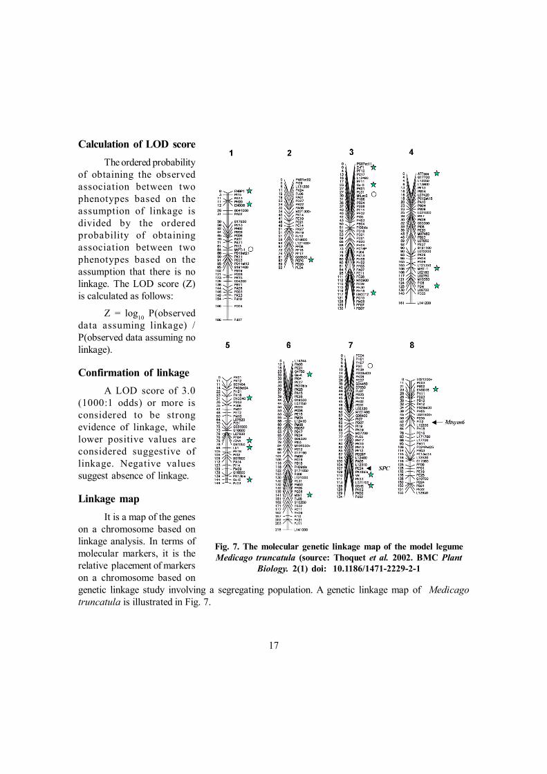
Calculation of LOD scoreThe ordered probability

of obtaining the observedassociation between twophenotypes based on theassumption of linkage isdivided by the orderedprobability of obtainingassociation between twophenotypes based on theassumption that there is nolinkage. The LOD score (Z)is calculated as follows:

Z = log10 P(observeddata assuming linkage) /P(observed data assuming nolinkage).

Confirmation of linkageA LOD score of 3.0

(1000:1 odds) or more isconsidered to be strongevidence of linkage, whilelower positive values areconsidered suggestive oflinkage. Negative valuessuggest absence of linkage.

Linkage mapIt is a map of the genes

on a chromosome based onlinkage analysis. In terms ofmolecular markers, it is therelative placement of markerson a chromosome based ongenetic linkage study involving a segregating population. A genetic linkage map of Medicagotruncatula is illustrated in Fig. 7.

Fig. 7. The molecular genetic linkage map of the model legumeMedicago truncatula (source: Thoquet et al. 2002. BMC Plant

Biology. 2(1) doi: 10.1186/1471-2229-2-1

18

Construction of linkage mapsConstruction of genetic map can be very interesting as during map construction one can

gather data, which is useful in systematic or evolutionary studies. Segregation analysis can beapplied with segregating population that is derived from a common set of ancestors. Genetic linkagemaps should not be confused with physical genomic maps, which can be obtained by determiningthe DNA sequence of chromosomes. Linkage maps and physical maps are related, but this relationis usually non-linear. The molecular maps are not important by itself in plant breeding. It is onlyuseful when it is used in conjunction with analysis of conventional markers. Few examples oflinkage maps in pulses are discussed hereunder.

Bharadwaj et al. (2010) developed a chickpea genetic linkage map by using sequence taggedmicrosatellite markers from a desi x kabuli F2 population. Thirty three loci were distributed over adistance of 471.1cM with an average marker density of 14.2 cM. A microsatellite enriched libraryof chickpea was constructed from putative SSR clones (Gaur et al. 2011). Total 254 STMS primerswere screened in a RIL population derived from ICCV 2 × JG 62 cross for generating new markerswhich improved the marker density and saturation of linkage in the vicinity of sfl (double podding)gene by integrating newly identified markers with that of previously developed chickpea intra-specific map. A genetic linkage map of the Lathyrus sativus was developed with 92 backcrossindividuals derived from a cross (ATC 80878 × ATC 80407) using 47 RAPD primers, 7 sequence-tagged microsatellite site and 13 STS/CAPS markers (Skiba et al. 2004). Two QTLs were associatedwith ascochyta blight resistance.

Gene mappingOne of the recent applications of new techniques of molecular biology is the rapid development

in gene mapping. Use of DNA based markers is allowing researchers to determine the sequenceof genes along chromosomes and the distances between them. These techniques are providingmethods to mark, and in some cases, sequence genes that are related to genetic traits such asdisease resistance or fruit colour. If genes can be identified, sequenced and cloned, gene transfertechniques can be used to transfer them to other species. With the available techniques it is possibleto link markers on a genetic map with traits of interest in a particular species. Although much of theinitial research effort has been applied to important cereal species, these techniques will have asignificant impact on pulses breeding. If a genetic marker can be obtained for a trait of interest,plants could be selected at the seedling stage thereby saving many years at each step in a breedingprogramme. In constructing genetic maps, the amount of information generated depends on threefactors: completeness of detection of recombinational events, linkage distance between loci andnumber of individuals assayed. The first two factors are influenced by selection of parents forpopulation construction and markers used. More polymorphism between parents and the utilizationof more informative markers increases the number of loci that can be mapped. Generally, the

19

selection of parents for genetic map construction is optimized for maximum polymorphism betweenthe parents. However, for specific applications such as gene tagging, where a specific population isused, the level of polymorphism may not be as high as for the initial mapping population.

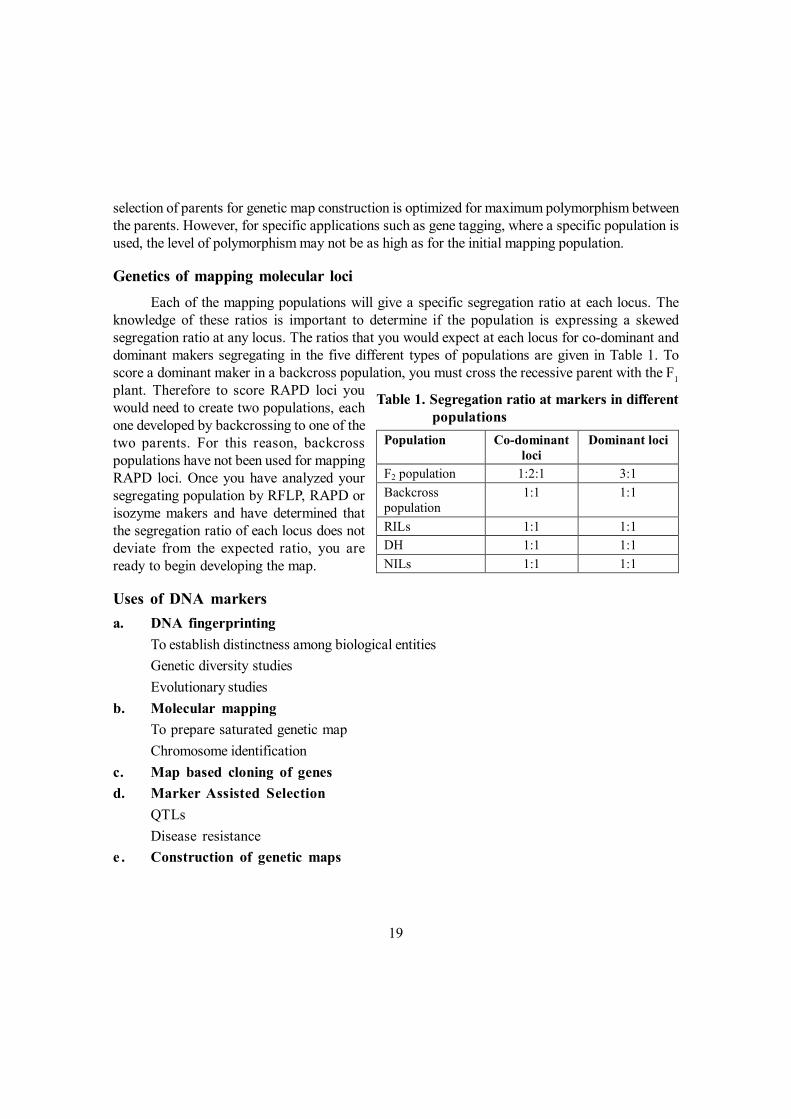
Genetics of mapping molecular lociEach of the mapping populations will give a specific segregation ratio at each locus. The

knowledge of these ratios is important to determine if the population is expressing a skewedsegregation ratio at any locus. The ratios that you would expect at each locus for co-dominant anddominant makers segregating in the five different types of populations are given in Table 1. Toscore a dominant maker in a backcross population, you must cross the recessive parent with the F1plant. Therefore to score RAPD loci youwould need to create two populations, eachone developed by backcrossing to one of thetwo parents. For this reason, backcrosspopulations have not been used for mappingRAPD loci. Once you have analyzed yoursegregating population by RFLP, RAPD orisozyme makers and have determined thatthe segregation ratio of each locus does notdeviate from the expected ratio, you areready to begin developing the map.

Uses of DNA markersa. DNA fingerprinting

To establish distinctness among biological entitiesGenetic diversity studiesEvolutionary studies

b. Molecular mappingTo prepare saturated genetic mapChromosome identification

c. Map based cloning of genesd. Marker Assisted Selection

QTLsDisease resistance

e . Construction of genetic maps

Table 1. Segregation ratio at markers in differentpopulations

Population Co-dominant loci

Dominant loci

F2 population 1:2:1 3:1 Backcross population

1:1 1:1

RILs 1:1 1:1 DH 1:1 1:1 NILs 1:1 1:1

20

Materials required for construction of a genetic mapMapping population and molecular markers are required for constructing a genetic map.

Linkage estimation is based on segregation of markers. Huge data are generated but softwarepackages available to calculate linkage. Saturation of genetic map depend on completeness ofdetection of recombination events; linkage distance between loci; number of individuals assayed.Polymorphic parents and more informative markers increase the number of loci that can be mapped

Quantitative trait loci (QTL) QTLs are short segments of DNA (locus) that have some contribution towards the phenotypic

value of quantitative traits. Such locus may carry single or group of genes that are tightly linked andmostly inherited together. Many such loci determine the total phenotypic value of the trait (e.g.,yield). Each of these loci are called QTLs. Major QTLs are those loci that have major impact onthe phenotypic value, whereas minor QTLs have minor impact on the phenotypic value. In QTL-mapping, association between observed trait values and presence/absence of alleles of markers,that have been mapped onto a linkage map is analysed. When it is significantly clear that thecorrelation that is observed did not result from some random process, it is proclaimed that a QTL isdetected. In addition, the size of the allelic effect of the detected QTL can be estimated.

Basic steps in QTL analysis Make cross and generate mapping population

Identify markers that are polymorphic between the parents

Generate marker data

Generate linkage maps of molecular markers

Collect phenotypic measurements of QTL trait

Map QTLs (Association of QTL with marker).

QTLs analysis

Scoring individuals of a random segregating population for a QTL trait is done by growing thesegregating population in replicated multi-location trials. Determination of the molecular genotype/DNA marker data of each member of the segregating population is done by analyzing the DNAwith specific markers. Specific programmes are prepared (with certain theoretical assumptions)for determining association between any of the markers and the quantitative trait. Therefore,experimental procedure must comply with these assumptions.

21

Methods of determining association of QTL and trait Single marker test

Interval mapping

Composite interval mapping

Multiple interval mapping

Statistical procedures in marker assisted selectionStatistical applications in biotechnology have increased tremendously in recent years. With

the help of statistical software a researcher may identify statistically significant differences in asingle variable; between two or more groups and design efficient single factor experiments, whichare fit for purpose and economical with scarce experimental resource. Statistical procedures arealso required to fit simple calibration curves to biological data, produce informative data summariesfor experiments with measurements on multiple variables, compare proportions between two ormore groups, identify sources of variability in an experiment and design efficient experiments withappropriate choice of the number of replicates and level of replication, analyze data from experimentswith multiple factors and to compare the response profiles on multiple variables between groups.

CorrelationCorrelation usually refers to the degree to which a linear predictive relationship exists between

random variables, as measured by a correlation coefficient. Correlation is a statistical procedureused to determine the degree to which two (or more) variables vary together. Correlation does notsuggest a cause-effect relationship but only the degree of parallelism or concomitance between thevariables, the cause of which may be unknown. The Pearson product-moment correlation (r) isthe most frequently used, and this coefficient is used unless another is specified. Correlation maybe positive or negative.

Cluster analysisGiven a set of varieties each of which belongs to one set of class, the statistical/computational

techniques used to place the objects in the class to which they belong is called cluster analysis. Ifthe classes are known it is mere classification. If the classes are not known then it is a problem. forexample, given a set of DNA finger print profiles, along with the information that they belong todifferent species of rice except that the origin of some of the finger prints is not known, a clusteranalysis can be used to classify the finger print according to species and possibly discover thespecies identity of the unlabelled finger print. In order to find the clustering relationships among a

22

set of objects it is crucial that we must have the dissimilarities or similarities among them. So themeasurement of similarity of finger printing is of very important in population genetics. When DNAprofiles of two individual plants are compared, a certain number of bands will be common (shared)between the two profiles, even by chance. The number or proportion of shared bands is expectedto be larger if the two individuals are biologically related. It is, therefore, important to objectivelymeasure the expected degree of similarity due to chance or relatedness.

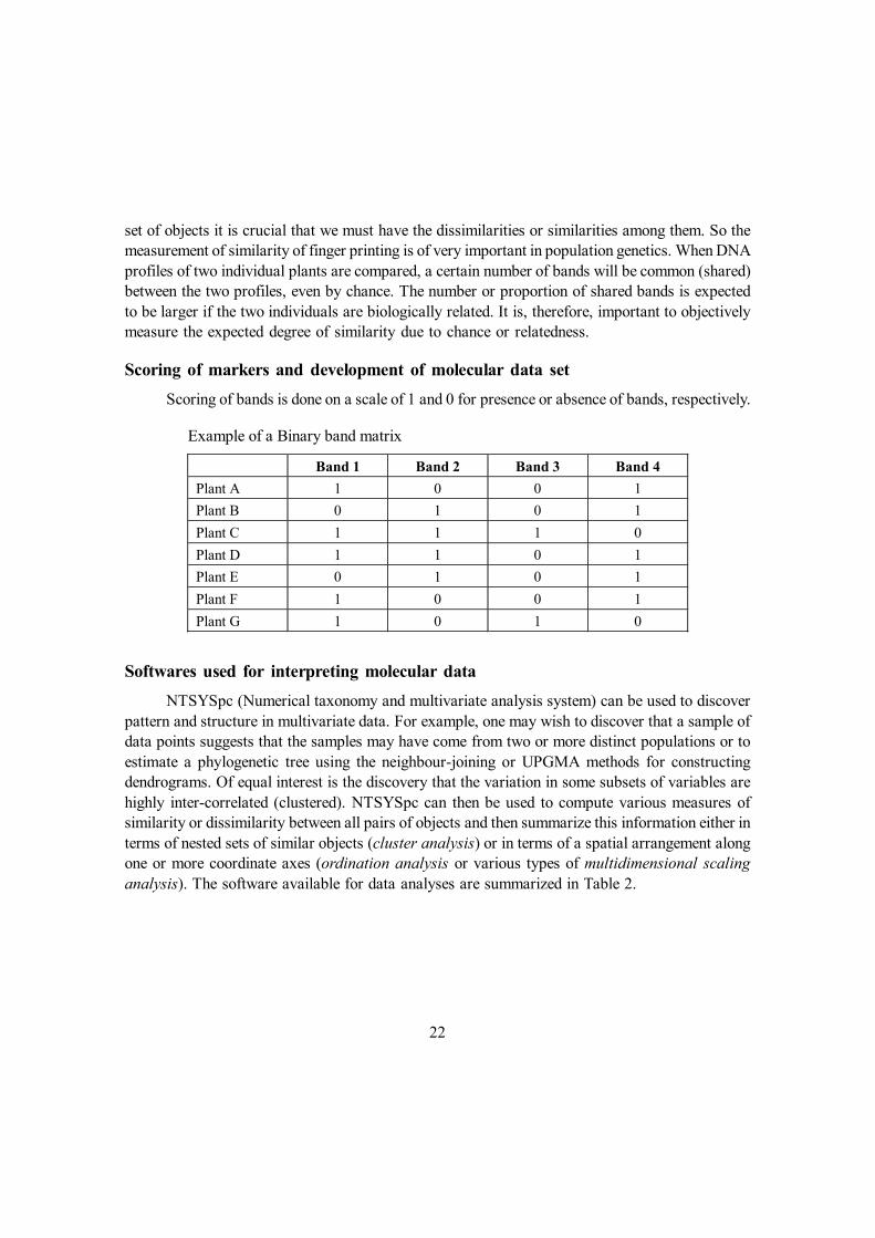
Scoring of markers and development of molecular data setScoring of bands is done on a scale of 1 and 0 for presence or absence of bands, respectively.

Softwares used for interpreting molecular dataNTSYSpc (Numerical taxonomy and multivariate analysis system) can be used to discover

pattern and structure in multivariate data. For example, one may wish to discover that a sample ofdata points suggests that the samples may have come from two or more distinct populations or toestimate a phylogenetic tree using the neighbour-joining or UPGMA methods for constructingdendrograms. Of equal interest is the discovery that the variation in some subsets of variables arehighly inter-correlated (clustered). NTSYSpc can then be used to compute various measures ofsimilarity or dissimilarity between all pairs of objects and then summarize this information either interms of nested sets of similar objects (cluster analysis) or in terms of a spatial arrangement alongone or more coordinate axes (ordination analysis or various types of multidimensional scalinganalysis). The software available for data analyses are summarized in Table 2.

Example of a Binary band matrix

Band 1 Band 2 Band 3 Band 4 Plant A 1 0 0 1 Plant B 0 1 0 1 Plant C 1 1 1 0 Plant D 1 1 0 1 Plant E 0 1 0 1 Plant F 1 0 0 1 Plant G 1 0 1 0

23

Application Interval mapping, multiple QTL modeling Population F2 backcross, RIL, DH

MAPMANAGER

Language Unix Application Interval mapping using non linear regression Population F2 backcross, RIL, DH

QTLSTAT

Language Unix Application t-test, conditional t-test, linear regression Population F2 backcross, RIL, DH, F1, OP

PGRI

Language Unix Application t-test, Composite Interval mapping, permutation test,

bootstrap, jackknife

Population F2 backcross, RIL, DH

QTL Cartographer

Language Unix/Mac/PC Windows Application Interval mapping, MQM Population F2 backcross, RIL, DH, F1

MAPQTL

Language Vax/Unix/Mac/ PC Windows Application Interval mapping using regression, MQM

Population F2 backcross

Map Manager QT

Language MAC OS Application linear regression Population F2 backcross

QGENE

Language MAC

Table 2. Softwares and their application in molecular breeding

24

Use of Molecular Markers in Breeding Programmes

Marker aided selection is a tool for breeding, wherein genetic marker(s) tightly linked withthe desired trait/gene(s) are utilized for indirect selection for that trait in segregating/non-segregatinggenerations. In its simplest form it can be applied to replace evaluation of a trait that is difficult orexpensive to evaluate. When a marker is found that co-segregates with a major gene for an importanttrait, it may be easier and cheaper to screen for the presence of the marker allele linked to the gene,than to evaluate the trait. From time to time the linkage between the marker and the gene shouldthen be verified. When more complex, polygenic controlled traits are concerned, the breeder isfaced with the problem how to combine as many as possible beneficiary alleles for the QTLs thatwere detected. In this case, the breeding material can be screened for markers that are linked toQTLs. Based on such an analysis specific crosses can be devised for creation of an optimalgenotype by combining QTL alleles from different sources. Marker assisted selection, when appliedwithin the current breeding material to enhance a breeding programme, does not solve the problemof limited genetic variability that is often seen in breeding stocks. A different application of markerassisted selection could contribute to a genetic enrichment of breeding material. Marker assistedselection may be used to facilitate a controlled inflow of new genetic material. The wild speciesoften carries desired components that may be missing in cultivated material. Such components canbe transferred to elite cultivated material by repeated backcrossing. However, breeders are oftenreluctant to apply this method because of unpredictable linkage drag. These are caused by othergenes, which are unintentionally transferred along with the genes that control the target trait. It maytake considerable effort and screening to get rid of the unwanted genes and return the material toan acceptable agronomic value. Markers can be used to pinpoint the genetic factors that areresponsible for the desired characteristics in the unadapted material. In a backcross programme,the presence of the desired QTL alleles can be verified continuously by observing linked markers.

Marker assisted selection (MAS)MAS is most useful for traits that are difficult to select e.g., disease resistance, salt tolerance,

drought tolerance, heat tolerance, quality traits (aroma of basmati rice, flavour of vegetables). Theapproach involves selecting plants at early generation with a fixed, favourable genetic backgroundat specific loci, conducting a single large scale marker assisted selection while maintaining as muchas possible the allelic segregation in the population and the screening of large populations to achievethe objectives of the scheme. No selection is applied outside the target genomic regions, to maintainas much as possible the Mendelian allelic segregation among the selected genotypes. Afterselection with DNA markers, the genetic diversity at un-selected loci may allow breeders to generatenew varieties and hybrids through conventional breeding in response to targets set in breedingprogramme.

25

Material required for MASMolecular markers, a set of authentic lines carrying trait of interest and a population to

validate the markers to be used e.g., F2 or BCF2 for each of the individual traits/genes. Followingare the basic pre-requisites for MAS : Search of molecular markers that are linked to the trait of interest Validate the available markers in parents and breeding population If markers are not available, it has to be designed and validated before use (if mapping

populations are not available in hand it may take 2-4 years to generate and validate markers) Design a selection scheme and breeding strategy Fix the minimum population to be assayed to capture all beneficial alleles Meticulous record keeping Progeny testing for fixation of traits.

Steps involved in MAS1. Validation of molecular markers. Extract the DNA from test individuals and find out whether

there is one to one relationship with marker and the trait.2. Extract the DNA of breeding population at the seedling stage and apply MAS. Select the

individuals on the basis of presence of desired molecular markers for the concerned trait.For other traits, selection is based on classical breeding methods. Minimum individuals to beassayed should be as per the defined strategy and statistical considerations.

Limitations of MAS Cost factor Requirement of technical skill Automated techniques for maximum benefit Per se, DNA markers are not affected by environment but traits may be affected by the

environment and show G x E interactions. Therefore, while developing markers, phenotypingshould be carried out in multiple environments and implications of G x E should be understoodand markers should be used judiciously.

DNA marker has to be validated for each of the breeding population. Any apriori assumptionregarding the validity of markers may be disastrous.

Marker assisted backcross breedingA backcross breeding programme is aimed at gene introgression from a “donor” line into the

genomic background of a “recipient” line. The potential utilization of molecular markers in such

26

programmes has received considerable attention in the recent past. Markers can be used to assessthe presence of the introgressed gene (“foreground selection”) when direct phenotypic evaluationis not possible, or too expensive, or only possible late in the development. Markers can also be usedto accelerate the return to the recipient parent genotype at other loci (“background selection”). It isassumed that the introgressed gene can be detected without ambiguity, and the theoretical studywas restricted to background selection only. The use of molecular markers for background selectionin backcross programmes has been tested experimentally and proved to be very efficient.Introgressing the favourable allele of QTL by recurrent backcrossing can be a powerful mean toimprove the economic value of a line, provided the expression of the gene is not reduced in therecipient genomic background. Yet, recent results show that for many traits of economic importanceQTLs have rather small effects. In this case, the economic improvement resulting from theintrogression of the favourable allele at a single QTL may not be competitive when compared withthe improvement resulting from conventional breeding methods over the same duration. Markerassisted introgression of superior QTL alleles can then compete with classical phenotypic selectiononly if several QTLs could be manipulated.

Selection scheme for MAS breedingThe approach involves selecting plants at early generation with a fixed, favourable genetic

background at specific loci, conducting a single large scale marker assisted selection while maintainingas much as possible the allelic segregation in the rest of the genome. First, the identification of elitelines presenting high allelic complementarity and being outstanding for traits of interest is requiredto capture favourable alleles from different parental lines. Second, after identification of the mostfavourable genomic regions for each selected parental line, those lines are intercrossed to developsegregating populations from which plants homozygous for favourable alleles at target loci areselected. One objective of the scheme is to conduct the marker assisted selection only once, and itrequires the selection of a minimum number of plants to maintain sufficient allelic variability at theunselected loci. Therefore, the selection pressure exerted on the segregating population is quitehigh and the screening of large populations is required to achieve the objectives of the scheme. Noselection is applied outside the target genomic regions, to maintain as much as possible the Mendelianallelic segregation among the selected genotypes.

Application of DNA markers in crop improvement

QTL mapping

Some of the most difficult tasks of plant breeders relate to the improvement of traits thatshow a continuous range of values. Genetic factors that are responsible for a part of the observedphenotypic variation for a quantitative trait are called quantitative trait loci (QTLs). The term QTLwas coined by Gelderman. Conceptually it can be a single gene or may be a cluster of linked genesof the trait. Although similar to a gene, a QTL merely indicates a region on the genome comprised

27

of one or more functional genes. Among such quantitative traits like yield, plant length and days toflowering etc., are important ones. Selection for quantitative traits is difficult, because the relationbetween observed trait values in the field (the phenotype) and the underlying genetic constitution(the genotype) is not straight forward. Quantitative traits are typically controlled by many genes,each contributes only a small part to the observed variation. The environmental variations resultingfrom differences in growing conditions, further create the problem to understand the relation betweenphenotype and genotype. In practice, this problem is typically dealt with by evaluating large andreplicated trials, which allow identification of genotypic differences through statistical analysis.Plant breeders would like to utilize the quantitative traits for genetic factors that are responsible forthe observed variability in quantitative traits. In a process called QTL mapping, association betweenobserved trait values and presence/absence of alleles of markers, that have been mapped onto alinkage map is analysed. When it is significantly clear that the correlation that is observed did notresult from some random process, it is proclaimed that a QTL is detected. Also the size of the alleliceffect of the detected QTL can be estimated. Identification of molecular makers associated withQTLs involves three basic steps namely, scoring individuals of a random segregating population fora QTL trait; determination of the molecular genotype of each member of the population anddetermination of association between any of the markers and the quantitative trait. The first step isto make cross and generate marker data. In the next step generate linkage maps of molecularmarkers. Subsequently collect phenotypic measurements of QTL trait across the environments inreplicated trials. Finally, mapping of QTL is done. The most common method of determining theassociation between marker and QTL is done by analyzing phenotypic observation of trait andscoring of molecular data by one-way analysis of variance and regression analysis. For each marker,presence of a specific fragment of DNA is considered a marker class, and all individuals (in asegregating population) possessing that marker class are considered to be positive for that class. Ifthe variance due to a particular class is significant, then the molecular marker used to define, thatclass is considered to be associated with a QTL. Regression values are calculated for all themarkers which have shown association with the quantitative trait which reflect the amount of totalgenetic variation that is explained by the specific molecular marker. There are very few examplesof QTL mapping in pulse crops.

In chickpea, two RIL populations were used to construct a composite linkage map with thehelp of RAPD, ISSR, RGA, SSR and ASAP markers (Radhika et al. 2007). Marker trait associationwas observed among three yield related traits: double podding, seeds per pod and seed weight. Thedouble podding gene was tagged by the markers NCPGR 33 and UBC 249z. Seeds per pod wastagged with TA 2x and UBC 465 markers. Eight QTLs were identified for seed weight.

Duran et al. ( 2002) developed a QTL map for plant height, pod dehiscence, number ofshoots and seed diameter from inter-subspecific population of Lens culinaris ssp culinaris x Lensculinaris ssp orientalis. Tullu et al., (2008) identified QTLs in lentil for earliness and plant heightwith RAPD, SSR and AFLP markers. Kahraman et al. (2004) identified five independent QTLs

28

for winter hardiness in a population of RILs derived from a cross between lentil accessions WA8649090 x Precoz. One IISR marker Ubc 808-12 was found to be useful in MAS for predictingwinter survival in segregating populations. Rubeena et al. (2003) identified eight QTLs for ascochytablight resistance gene in lentil through composite interval mapping. Five QTLs were identified in F2population of ILL 5588/ILL 7537 whereas three QTLs were detected in F2 of the cross ILL 7537/ILL 6002.

Young et al. (1993) identified three QTL associated with powdery mildew resistance inmungbean, while Chaitieng et al. (2002) and Humphry et al. (2003) found one QTL responsible forpowdery mildew resistance in Vigna species. Sholihin and Hautea (2002) identified six AFLPderived putative QTLs associated with two traits (leaf relative water content and leaf stress rating)used to measure draught tolerance.

Tagging of disease resistance genesDNA based markers have shown great promise in expediting plant breeding methods. The

identification of molecular markers closely linked with resistance genes can facilitate expeditiouspyramiding of major genes into elite background, making it more cost effective. Once the resistancegenes are tagged with molecular marker the selection of resistant plant in the segregating generationsbecomes easy. A chickpea linkage map was established with help of 354 molecular markers (118STMSs, 96 DAFs, 70 AFLPs, 37 ISSRs, 17 RAPDs, eight isozymes, three cDNAs, two SCARsand three markers linked to fusarium wilt resistance) surveyed among 130 recombinant inbred linesderived from a C. arietinum × C. reticulatum (Winter et al.2000). The fusarium wilt resistantgenes for race 4 and 5 were placed on the linkage group that also contained STMS and a SCARmarker previously shown to be linked to fusarium wilt race 1. This is an indication of clustering ofseveral fusarium wilt resistance genes. These markers will pave the way for MAS and searchingother useful genes.

DNA markers associated with two closely linked genes for resistance to fusarium wilt race4 and 5 in chickpea were identified from a population of 131 recombinant inbred lines derived froma wide cross between Cicer arietinum and Cicer reticulatum (Benko-Iseppon et al. 2003). Withthe aid of bulk segregant analysis nineteen new markers were identified in the vicinity (4.1-9 cM)of fusarium wilt resistance genes on linkage group 2, R-2609-1 showed closest linkage (2cM) withrace 4 resistance locus. Gowda et al. (2009) identified flanking markers for chickpea fusarium wiltresistance genes in a recombinant inbred line population. H3A12 and TA101 SSR flanked the Foc1 resistance gene whereas Foc 2 was mapped between TA96 and H3A12. The H1B06y andTA194 markers flanked the Foc3 locus.

Reddy et al., (2009) performed bulk segregant analysis on a segregating population ofICPL 7035 x ICPL 8863 for identification of RAPD markers associated with pigeonpea sterilitymosaic disease (PPSMD) resistance. The primer OAP18 revealed polymorphism between the

29

parents and the resistant and the susceptible bulks. The OAP18 marker was converted into SCARmarker for identification of PPSMD resistant plants in the segregating population.

Dhanasekhar et al. (2010) identified two RAPD markers OPF04700 and OPA091375 werelinked with the open and tall plant type gene in pigeonpea F2 population of the cross between TT44-4 and TDI2004-1through bulk segregant analyses . These markers were validated in 15 genotypeswith open-tall plant type. Kotresh et al. (2006) used bulk segregant analysis with 39 RAPD primerswhich led to identification of two markers (OPM03704 and OPAC11500) that were associated withFusarium wilt susceptibility allele in a pigeonpea F2 population derived from GS1 x ICPL87119.

Taran et al. (2003) identified two molecular markers associated with Ascochyta blightresistance in lentil viz., UBC 2271290 linked with ral1 gene and RB18680 linked with AbR1 and amarker (OPO61250) linked with Anthracnose resistance gene were utilized for identifying linesthat possessed pyramided genes in a population of 156 recombinant inbred lines (RILs) developedfrom a cross between ‘CDC Robin’ and a breeding line ‘964a-46’. These markers can be convertedinto more robust SCAR markers for routine use in marker assisted selection. Tullu et al. (2003)tagged anthracnose resistance gene LCt-2 of lentil cultivar PI 320937 with RAPD and AFLPmarkers.

Basak et al. (2004) developed molecular marker linked to yellow mosaic virus (YMV)resistance gene in Vigna sp. from a population segregating for YMV disease resistance. Maiti etal. (2010) identified molecular markers CYR1and YR4 in a F2 population for screening of MYMIVresistance genes. CYR1 co-segregated with MYMV resistance gene in F2 plants and F3 progenies.These two markers can be used simultaneously with the help of a multiplex PCR reaction.

Katoch et al. (2009) identified a powdery mildew resistance gene er2 in pea that wasassociated with a RAPD marker OPX-17_1400, exhibiting cis phase linkage (2.6 cM) in a F2population derived from Lincoln/JI2480. The reproducibility of RAPD marker was enhanced byconverting it to a sequence characterized amplified region (SCAR) marker. Ek et al. (2005) usedbulk segregant analysis on a F2 population derived from the cross 955180 x Majoret for screeningof SSR markers linked with powdery mildew resistance gene in pea. Out of 315 markers, only fiveshowed linkage with the PM resistance gene. It was noted that none of single marker was tightlylinked with the gene that can be considered optimal for inclusion in a MAS program. Therefore, acombination of two markers can be utilized for selecting PM resistant plants which would result inonly 1.6% false positives.

Nguyen et al. (2001) converted a RAPD marker into a SCAR(SCARW19) for selectingascochyta blight resistance gene of lentil accession ILL5588. Rubeena et al. (2003) identifiedQTLs for ascochyta blight resistance in lentil. Further validation is required to use these markersfor MAS.

Hamwieh et al. (2005) mapped microsatellite markers identified from a genomic library oflentil. The linkage spanning about 751cM, consisting of 283 marker loci was derived from 86

30

recombinant inbred lines derived from the cross ILL 5588 × L 692-16-1(s) using 41 microsatelliteand 45 amplified fragment length polymorphism markers. The average marker distance was 2.6 cM.Two flanking markers (SSR marker SSR59-2B at 8.0 cM and AFLP marker p17m30710 at 3.5 cM)were linked with fusarium resistance.

Saxena (2010a) assessed the DNA polymorphism in a set of 32 pigeonpea lines screenedwith 30 SSR markers. Based on polymorphism of marker alleles, higher genetic dissimilaritycoefficient and phenotypic diversity for Fusarium wilt and sterility mosaic disease resistance data,five parental combinations were identified for developing genetically diverse mapping populationssuitable for the development tightly linked markers for Fusarium wilt and sterility mosaic diseaseresistance.

Tagging of male sterility genesA cytoplasmic male sterile system is desirable for use in hybrid seed production, as it eliminates

the need for hand emasculation. CMS is a maternally inheritable trait characterized by the inabilityto produce viable pollen but without affecting the female fertility, and it is often associated withmitochondrial DNA rearrangements, mutations and editing. Several restorer locus have been identifiedusing RAPD and STS in different crop and DNA markers linked to these locus enable the molecularstudy of the CMS system. These co-dominant markers are useful in identifying the homozygousrestorer genotypes after the backcrossing for production of restorer lines. In this way, the restorerlines could be produced in a shorter period than by conventional methods. Souframanien et al.(2003) identified RAPD marker linked with male sterility gene. Primer OPC-11 produced a uniqueamplicon of 600bp in male sterile (A) lines 288A (derived from C. scarabaeoides) and 67A (derivedfrom C. sericeus), which was absent in their respective, maintainers and putative R lines (TRR 5and TRR 6). Genetic distance based on similiraty index revealed considerable genetic variationbetween male sterile lines, two putative R lines and donors of male sterility genes.

Diversity evaluationStability and identity of crop variety has assumed great importance for predicting plant

breeder’s right/farmers right. Traditionally, evaluation and conservation of bio-diversity/geneticvariability is based on comparative anatomy, morphology, embryology, physiology, etc., which provideinformative data but of low genetic resolution. Recent advances in molecular biology have providedpowerful genetic tools, which can provide rapid and detailed genetic resolution. Molecular markerbased genotyping involves the development of marker profile unique to an individual. Thisunambiguous pattern of crop varieties obtained using DNA a marker is termed as “DNAFingerprinting”. The technique was developed by Alec Jeffery in 1985 in human and was used firsttime in crop (rice) in 1988 by Dallas for cultivar identification. The choice of molecular marker tobe used for DNA fingerprinting usually depends on technical expertise, available funds as well asthe requirements of the experiment. At the same time the most important considerations in the use

31

of molecular techniques are discrimination power and reproducibility. RAPD markers have shownto be of low discrimination power as compared to SSR and AFLP. Now days, microsatellites arethe method of choice for varietal identification due to their abundance, high polymorphism, andsimple protocol etc. Odeny et al. (2007) deduced DNA polymorphism in pigeonpea by using 113primers (designed from genomic SSR) and 220 soybean primers.

Sivaramakrishnan et al. (2002) showed that RFLP of mtDNA can be used for the diversityanalysis of pigeonpea. They assayed restriction enzyme digested fragments of 28 accessionsrepresenting 12 species of the genus, Cajanus arranged in 6 sections including 5 accessions of thecultivated species C. cajan and 4 species of the genus Rhyncosia with maize mtDNA probes. Inaddition to inter-specific variability, intra-specific diversity was observed between the accessionsof wild species (C. scarabaeoides, C. platycarpus, C. acutifolius) and cultivated species of C.cajan.

Saxena et al. (2010b) designed 23 primer pairs from 36 SSR enriched genomic library ofpigeonpea. Sixteen primer pairs produced expected amplification fragments, of which 13 werepolymorphic amongst 32 cultivars and 8 wild accessions representing six species. The averagepolymorphic information content was 0.32 per marker which varied from 0.05 to 0.55 for these 13primer pairs.

Ratnaparkhe et al. (1995) developed DNA fingerprints for cultivated and wild pigeonpeaaccessions with the help of RAPD markers. The polymorphism among the cultivated species waslow whereas high level of polymorphism was observed among the wild species. All pigeonpeaaccessions including cultivars under study were distinguishable from each other which demonstratedutility of RAPD in the genetic fingerprinting of pigeonpea. Ganapathy et al. (2011) generated 561amplified fragment length polymorphism (AFLP) loci for clustering cultivated and wild pigeonpeaaccessions. Jaccard’s similarity index indicated greater diversity within wild species which clusteredinto several groups. Most of the cultivated accesions were grouped into one major cluster. Amongthe cultivated lines, BRG 3, ICP 7035, TTB 7 and ICP 8863 were selected on the basis ofmorphological and molecular diversity for generating mapping population for identification of markerslinked to sterility mosaic disease.

Hamwieh et al. (2009) developed new set of microsatellite markers in lentil for delineatingthe molecular diversity. Souframanien and Gopalkrishna (2004) used RAPD and IISR markers fordeducing the genetic diversity among 18 blackgram cultivars.

Heterosis breedingAnother important application of DNA markers is their prediction of heterosis in hybrids.

Evaluation of hybrids for heterosis or combining ability in field is expensive. Molecular markershave been used to correlate genetic diversity and heterosis in several cereal crops (like rice, oat,and wheat). It has been reported that measures of similarity based on RFLP and pedigree knowledge

32

could be used to predict superior hybrid combinations. However, both low and high correlationsbetween heterosis and DNA based genetic distance have been observed.

The correlation between heterosis and molecular (isozyme and RFLP) diversity between theparents was investigated in three maturity groups in soybean (Cern et al. 1997). Parental RFLPdiversity was not significantly correlated with mid parent and better parent heterosis indicating thatheterosis in yield may not be associated with genetic diversity at the molecular level as determinedby RFLPs. Though isozyme diversity in parents was associated with yield heterosis, it is of limitedimportance because of the reduced number of assayable isozyme loci in soybean.

Hybrid seed purity testingTo determine the hybrid seed quality it is to be verified that the designated cross has occurred,

the number of self pollination between the female parents meet the necessary purity and the producthas adequate quality. For years, the only method to check the hybrid seed purity has been the growout test. Now the RAPD and RFLP are markers are used to test the purity of F1 hybrids. Kumar etal. (2011) used male specific markers SSR 218, SSR 306 and Ty2 gene CAPs gene marker testingF1 purity of Pbc × EC 538408, Pbc × EC 520061 and H 86 × EC 520061 tomato hybrids.

Gene pyramidingIt is essentially a way of determining and introducing multiple genes which impart resistance

to an independent insect/microbial pest, or impart resistance to a single pest through independenthost pathways. One strategy for increasing the durability of resistance is to incorporate multipleresistance genes into a single variety. If the pyramided genes have never been deployed as singlegenes, then it is estimated that the durability of resistance could be extended for 50 years. However,during the process of constructing a cultivar, it is difficult to verify the number of resistance genesthat have been successfully pyramided. Plants with only one resistance gene are just as resistant asplants that contain three resistance genes, although the resistance of the latter is probably moredurable.

Li et al. (2010) pyramided phytopthora tolerance QTLs in soybean. A recombination inbredline population was generated by crossing two phytopthora tolerant soybean cultivars Conrad andHefeng 25. With the help of 161 SSR markers, 7 environmentally stable QTLs (QPRR-1and QRR-2 Conard and QRR3 to QRR7 from Hefeng 25) were identified. The more the number of QTLs thehigher was the level of tolerance.

Pyramiding of Bt genesThe insecticidal cry (crystal) genes from Bacillus thuringiensis (Bt) have been used for

insect control both as biopesticides and in transgenic plants. Discovery of new insecticidal genes isof importance for delaying the development of resistance in target insects. The diversity of Bt

33

strains facilitates isolation of new types of cry and vip (vegetative insecticidal protein) genes. PCRis a useful technique for quick and simultaneous screening of Bt strains for classification andprediction of insecticidal activities. PCR together with other methods of analysis such as RFLP,gene sequence determination, electrophoretic, immunological and chromatographic analysis of Cryproteins and insect bioassays for evaluation of toxicity have been employed for identification ofnew insecticidal proteins. Some other new approaches have also been devised. Many Bt strainswith novel insecticidal genes have been found. A desired combination of Cry proteins can beassembled via site-specific recombination vectors into a recipient Bt strain to create a geneticallyimproved biopesticide. For better pest control, the cry genes have been transferred to plants.Stacking of more than one insecticidal gene is required for resistance management in transgeniccrops. Modification of Cry proteins through protein engineering for increasing the toxicity and/orthe insecticidal spectrum is also a promising approach, but requires detailed understanding of thestructure and function of these proteins and analysis of toxin-receptor interactions. Stringentimplementation of resistance management is needed for maintaining the efficacy of Bt transgeniccrops and deriving maximum economic and environmental benefit. cry1Ac and cry1C Bt geneswere incorporated in the Broccoli line (Cao et al. 2002). cry1Ac and cry1C mRNAs were detectedin the hybrid lines which also produced stable Cry1Ac and Cry1C proteins at levels comparable tothe parental plants carrying individual genes. Plants with pyramided cry genes did not show leafdamage and killed the DBM larvae resistant to Cry1A or Cry1C.

Map based cloning of genesThe first step of map-based or positional cloning is to identify a molecular marker that lies

close to the gene of interest. Initially gene search is done with a small mapping population andsubsequently, a highly saturated genetic map is prerequisite to clone a gene. With reference to aninitial marker, the region around that original molecular marker is saturated with high density markers.A large number of individuals are screened to find a marker which rarely recombines with the geneof interest. The next step is to screen a large insert genomic library (BAC or YAC) with thepreviously identified closely linked molecular markers to isolate clones that hybridize with the marker.Once two flanking markers that show linkage with the target gene are identified then the targetgene is searched with the help of chromosomal walking. The goal is to find clones harbouring a setof flanking markers that co-segregate with the gene of interest. Such putative clones are introducedinto the individuals devoid of the target gene. If a transgenic is shown to rescue the mutant phenotype,then detailed molecular and biochemical analysis of the newly cloned gene is undertaken tocharacterize the gene.

Map based cloning technique was employed to clone Pto (resistance to bacterial speckdisease of tomato) gene of tomato (Martin et al. 1993). Initially a genetic population of 251 F2plants was screened with DNA probes. The locus TG 538 cosegregated with Pto gene. A YAClibrary was screened with the TG 538 probe and the clone PTY538-1 was identified. Susceptibleplants transformed with PTY 538 recovered resistant phenotype.

34

Principles of Basic Techniques

Genomic DNA extractionThe method of DNA extraction from plant tissue generally varies depending on the material

used for isolation of DNA. Any mechanical means of breaking down the cell wall and membranesto allow access to nuclear material, without its degradation is essential. For this purpose, generallyan initial grinding with liquid nitrogen is employed to break down cell wall material and allow accessto DNA while harmful cellular enzymes and chemicals remain inactivated. Once the tissue hasbeen sufficiently ground to a fine powder, it can then be resuspended in a suitable buffer, such asCTAB. Later, insoluble particulates (cell debris) are removed through centrifugation, while solubleproteins and other material are separated through repeated mixing with chloroform and isoamylalcohol and centrifugation. DNA is then precipitated from the aqueous phase and washed thoroughlyto remove contaminating salts. The purified DNA can be resuspended and stored in TE buffer or insterile distilled water. The CTAB method has been shown to give intact genomic DNA from planttissues. To check the quality of the extracted DNA, a sample is run on an agarose gel, stained withethidium bromide, and visualised under UV light.

Quantification and quality check of DNA

UV quantification of DNA

Add 15 µl of each sample to 735 µl TE, mix well, and read OD 260 and OD 280 to determinepurity. After UV quantification, adjust the concentration of each DNA sample to 0.3 µg/µl or aconcentration of your choice with TE, and store at 4°C.

The ratio OD 260/OD 280 should be determined to assess the purity of the sample. If thisratio is in between 1.8-2.0, the absorption is probably due to nucleic acids. A ratio of less than 1.8indicates there may be proteins and/or other UV absorbers in the sample, in that case it is advisableto re-precipitate the DNA. A ratio higher than 2.0 indicates the samples may be contaminated withchloroform or phenol and should be re-precipitated with ethanol.

Approximate DNA quantification through gel electrophoresis

Make a 0.8% agarose gel with 1x TAE and 0.1µl of Ethidium bromide (10 mg/ml) per 10 mlsolution. Load one undiluted sample and dilutions, with 3µl loading buffer. Also include a DNAladder cut with HindIII and EcoRI. This contains 100 ng/µl of DNA and use as follows:

1µl ladder + 4µl water + 2µl loading buffer

2µl ladder + 3µl water + 2µl loading buffer

35

The different bands of the ladder are of known molecular weight and known DNAconcentration. Match the brightness of samples with those of the two dilutions of the ladder.Remember that although the ladder concentrations are absolute, you have loaded 5µl of sample andalso diluted some of them. This must be taken into account when calculating the strength of thesamples in çg/µl.

Assessment of DNA quality Prepare 0.8% solution of agarose by melting 1.0 g of agarose in 100 ml of 0.5x TBE buffer

for approximately 2 min. Allow to cool for a couple of minutes then add 2.5 µl of ethidiumbromide, stir to mix.

Cast a gel using the tray and comb. Allow the gel to set for a minimum of 20 min at roomtemperature on a flat surface.

Load 10 µl lkb ladder and 5 µl sample + 5 µl water + 2 µl 6x loading buffer into separate wells Run the gel for 30 min at 100 V Expose the gel to UV light and photograph Confirm DNA quality: presence of a highly resolved high molecular weight band indicates

good quality DNA, presence of a smear in the lane indicates DNA degradation.

DNA digestibility testThis step is essential before setting up large scale digestion experiments. A small amount of

DNA is digested with restriction endonucleases. Put 2 µg of each DNA sample in a 0.5 ml micro-centrifuge tube. Prepare a bulk digestion mix based on the recipe given below and keep it on ice. Add 8 µl of this to each of the tubes containing the DNA. Mix thoroughly but gently and spin

down the tube contents. Incubate at 37°C for 1.5 to 3 h. Stop the reactions with 3 µl of 5X SGB. Load samples in a 0.8% agarose gel and run the gel at 40 mAmp for 2-3 h. Use Lambda DNA digested with HindIII as a molecular weight marker.

Polymerase chain reaction (PCR)

Preparation of reaction mixture

To perform several parallel reactions, it is recommended to prepare a master mix containingwater, buffer, dNTPs, primers and Taq DNA polymerase in a single tube, thereafter, differentaliquots can be made for individual tubes. MgCl2 and template DNA solutions are then added. This

36

method of setting reactions minimizes the possibility of pipetting errors and saves time by reducingthe number of reagent transfers.

Reaction mixture set up1. Gently vortex and briefly centrifuge all solutions after thawing.2. Add, in a thin-walled PCR tube kept on ice:

3. Gently vortex the sample and briefly centrifuge to collect all drops from walls of tube.4. Overlay the sample with half volume of mineral oil or add an appropriate amount of wax.

This step may be omitted if the thermal cycler is equipped with a heated lid.5. Place samples in a thermocycler and start PCR.

Composition of the reaction mixture

a. Template DNA

Usually the template DNA amount is in the range of 0.01-1.0 ng for plasmid or phage DNAand 0.1-1.0 µg for genomic DNA, for a total reaction mixture of 50 µl. High template DNAconcentration generally increases the yield of non-specific PCR products, but if the fidelity ofsynthesis is crucial, maximal allowable template DNA quantities in conjunction with limiting numberof PCR cycles should be used to increase the percentage of “correct” PCR products. Nearly, allroutine methods are suitable for template DNA purification. Even trace amounts of agents used inDNA purification procedures (phenol, EDTA, Proteinase K, etc.) strongly inhibit Taq DNAPolymerase activity. Ethanol precipitation of DNA and repetitive treatments of DNA pellets with70% ethanol is usually effective in removing traces of contaminants from the DNA samples.

Reagent Final concentration

Quantity, for 25µl of reaction mixture

Sterile deionized water – Variable 10X PCR buffer 1X 2.5µl 25mM MgCl2 1-4mM Variable 2mM dNTP mix 0.2mM of each 2.5µl Primer I 0.1-1µM Variable Primer II 0.1-1µM Variable Taq DNA polymerase 0.5-1U/25µl Variable Template DNA 10pg-0.5µg Variable

37

b. Primers

PCR primers are usually 10-30 nucleotides in length. Longer primers provide sufficientspecificity. The GC content should be more than 50%. The C and G nucleotides should be distributeduniformly within the full length of the primer. More than three G or C nucleotides at the 3'-end ofthe primer should be avoided, as non-specific priming may occur. The primer should not be self-complementary or complementary to any other primer in the reaction mixture as this avoids primer-dimer and hairpin formation. The melting temperature of flanking primers should not differ by morethan 5°C, so the GC content and length must be chosen accordingly. All possible sites ofcomplementarity between primers and the template DNA should be noted. If primers are degenerate,at least 3 conservative nucleotides must be located at the primer’s 3'-end.

Estimation of the melting and annealing temperatures of primer: If the primer is shorter than25 nucleotides, the approx. melting temperature (Tm) is calculated using the following formula:

Tm = 4 (G + C) + 2 (A + T)

Annealing temperature should be approximately 5°C lower than the melting temperature. Ifthe primer is longer than 25 nucleotides, the melting temperature should be calculated using specializedcomputer programmes, where the interactions of adjacent bases, the influence of salt concentration,etc., are evaluated.

Primer quantity

a. Primer in pico-moles = weight in µg x 1000,000 Length of primer x 327

b. Micromolar concentration of primer = pico-moles/µlExample 1: Caculate the primer quantity if, 20 pmoles of primer is mixed in 100 µlPCR mixture

= 20 × 100 × 10–4 µM

= 0.20 µM

Example 2: How much 20 nt primer (con. 25 g/µl) is required for a 25 µl reactionmixture requiring 0.5 µM primer?

At first convert 25 g/µl in to pico-moles and then in to µM concentration

pmoles in 1 µl = 25x10-3x106

20x327

= 3.82 pmoles/µl

pmoles per µl is equivalent to µM concentration

38

Therefore, the concentration of primer is 3.82µM

Now, calculate the required quantity by N1V1 = N2V2

3.82x X= 0.5 x 25

X = 3.27µl

Therefore, the required quantity of primer is 3.27 µl

Example 3: What is the micromolar concentration of a primer of 26 nt lengthdissolved in 0.2ml of water?

The spectrophotometer reading of a 20µl aliquot diluted to 1ml is A260 = 0.82. The primerbase composition is A=6, T=6, C=7, G=7.

The stock solution is diluted 100 times (10 µl made to 1ml)

Therefore, the stock solution has an absorbance at 260 nm (A260) of 82

The Molar Extinction Coefficient at 260 nm for the primer = k (15,200) + I (12,010) + m(7,050) + n(8,400)

Where, k = number of A’s; m =number of C’s; I =number of G’s; n = number of T’s

The Molar Extinction of the Primer = 6 x 15,200 + 7 x 12,010 + 7 x 7,050 + 6 x 8,400 =275020

The Molar Concentration = 82/275020 = 298x10-6 molar =298 µM

c. MgCl2 concentration

Since Mg2+ ions form complexes with dNTPs, primers and DNA templates, the optimalconcentration of MgCl2 has to be selected for each experiment. Less quantity of Mg2+ ions resultsin a low yield of PCR product, and too many ions increase the yield of non-specific products andpromote misincorporation. Lower Mg2+ concentrations are desirable when fidelity of DNA synthesisis critical. Under the standard reaction conditions specified for most of the experiments, therecommended range of MgCl2 concentration is 1-4 mM. In general, at a final dNTP concentrationof 0.2mM, a MgCl2 concentration ranges of 1.5±0.25mM (in traditional PCR buffer) and of2.0±0.5mM (in PCR buffer with (NH4)2SO4) are suitable in most cases. If the DNA samplescontain EDTA or other chelators, the MgCl2 concentration in the reaction mixture should be raisedproportionally.

Example 4: How much 25 mM MgCl2 is required to make 2 mM of 25 µl reactionmixture?

Apply N1VI = N2V2

39

Units in RHS and LHS must be same

25 x X = 2x 25

X = 2 x 25 25

X = 2

Therefore, 2 µl MgCl2 is required.

d. dNTPs

The concentration of each dNTP in the reaction mixture is usually 200 µM. It is very importantto have equal concentrations of each dNTP (dATP, dCTP, dGTP, dTTP), as inaccuracy in theconcentration of even single dNTP dramatically increases the misincorporation. When maximumfidelity of the PCR process is crucial, the final dNTP concentration should be 10-50 µM. In addition,the concentration of MgCl2 should be selected empirically, starting from 1mM and increasing in0.1mM steps, until a sufficient yield of PCR product is obtained.

Example 5: How to make 1.0 ml of 1 mM dNTP from a stock of 100 mMdNTP?

100 x X = 1 x 1000

X = 10

Therefore, 10µl of each dNTP (dATP,dTTP dCTP dGTP) added to 960 µl of H2O.

Example 6: How much 1 mM dNTP is required to make 200 µM of 25 µlreaction mixture?

1000 x X = 200 x 25

X = 5

Therefore, 5µl dNTP is required.

e . Taq DNA Polymerase

Usually 1-1.5 U of Taq DNA polymerase is used in 50 µl of reaction mix. Higher Taq DNApolymerase concentration may cause synthesis of non-specific products. However, if inhibitors arepresent in the reaction mix (e.g., if the template DNA used is not highly purified), higher amount ofTaq DNA polymerase (2-3 U) is helpful in obtaining a better yield of amplification products.

Example 7: How much Taq DNA polymerase (5U/ µl) is required in a reactionrequiring 0.6 unit of Taq?

40

5 U ——— 1 µl

For 0.6U ——— 1 x 0.6 5

Therefore, 0.12 µl Taq DNA polymerase is required.

f. Temperature cycling

i. Initial denaturation step

The complete denaturation of the DNA template at the start of the PCR reaction is of keyimportance. Incomplete denaturation of DNA results in the inefficient utilization of template in thefirst amplification cycle and in a poor yield of PCR product. If the GC content is 50% or less, aninitial denaturation should be performed over an interval of 1-3 min at 95°C. This interval could beextended up to 10 min for GC rich templates. If the initial denaturation is no longer than 3 min at95°C, Taq DNA polymerase can be added into the initial reaction mixture. If longer initial denaturationor a higher temperature is necessary, Taq DNA Polymerase should be added only after the initialdenaturation, as the stability of the enzyme generally, decreases at temperatures over 95°C.

ii. Denaturation step

Usually 30 sec to 2 min denaturation at 94/95°C is sufficient, since the PCR productsynthesized in the first amplification cycle is significantly shorter than the template DNA and iscompletely denatured under these conditions. If the amplified DNA has a very high GC content,denaturation time may be increased up to 3-4 min. Alternatively, additives facilitating DNAdenaturation [e.g., glycerol (10-15 vol.%), DMSO (up to 10%), or formamide (up to 5%)] can beused. In the presence of such additives, the annealing temperature should be adjusted, since themelting temperature of the primer-template DNA duplex decreases significantly. If additives areused, the amount of Taq DNA polymerase in the reaction mix should be increased, because DMSOand formamide, at the suggested concentrations, reduces (inhibit) the enzyme activity by 50%.Alternatively, a common way to decrease the melting temperature of the PCR product is to substitutedGTP with 7-di-aza-dGTP in the reaction mix.

iii. Primer annealing step

Usually, the optimal annealing temperature is 5°C lower than the melting temperature ofprimer-template DNA duplex. Incubation for 30 sec to 2 min is sufficient. However, if non-specificPCR products are obtained in addition to the expected product, the annealing temperature shouldbe optimized by increasing it stepwise by 1-2°C.

iv. Extension step

The extension step is generally performed at 70-75°C. The rate of DNA synthesis by Taq

41

DNA polymerase is highest at this temperature (2-4 kb/min), and a 1 min extension time is sufficientfor the synthesis of PCR fragments of ~2 kb. When larger DNA fragments are to be amplified, theextension time is increased by 1 min for each 1000 bp.

v. Final Extension step

After the last cycle, the samples are usually incubated at 72°C for 5-15 min to fill-in theprotruding ends of newly synthesized PCR products. Also, during this step, the terminal transferaseactivity of Taq DNA polymerase adds extra A nucleotides to the 3’-ends of PCR products. Therefore,if PCR fragments are to be cloned into TA cloning vectors, this step can be extended for up to 30min.

vi. Number of cycles

The number of PCR cycles depends on the amount of template DNA in the reaction mix andon the expected yield of the PCR product. For less than 10 copies of template DNA, 40 cyclesshould be performed. If the initial quantity of template DNA is higher, 25-35 cycles are usuallysufficient.

How to avoid contamination during PCR? DNA sample preparation, reaction mixture assemblage, and the PCR process, in addition to

the subsequent reaction product analysis, should be performed in separate areas. A Laminar air-flow cabinet equipped with a UV lamp is recommended for preparing the

reaction mixture. Fresh gloves should be worn for each PCR setup. The use of dedicated vessels and positive displacement pipettes or tips with aerosol filters

for both DNA sample and reaction mixture preparation, is strongly recommended. The reagents for PCR should be prepared separately and used solely for this purpose.

Autoclaving of all solutions, except dNTPs, primers and Taq DNA polymerase is recommended.Solutions should be aliquoted in small portions and stored in designated PCR areas. Aliquotsshould be stored separately from other DNA samples.

A control reaction, omitting template DNA, should always be performed, to confirm theabsence of contamination.

Optimization of RAPD reactionRAPD reactions require optimization for getting better bands. For optimization, the reactions

are first carried out at an optimal PCR conditions. By varying the different variables one by one theamplification conditions are standardized. Reactions without DNA were used as negative controls.The standardization the reactions are generally carried out in a 25 µl reaction volume. Generally, a

42

standard reaction require about 50 g of template DNA, 1x PCR Buffer (10 mM Tris Hcl pH 8.3;50 mM KCl), 3 mM MgCl2, 0.2 mM dNTP Mix, 0.5 µM of single primer, 0.4 U of Taq DNApolymerase. The thermocycler may be programmed for an initial denaturation step of 3 min at94°C, followed by 30 cycles of 45 s at 94°C, 1 min at 37°C, extension was carried out at 72°C for1 min and final extension at 72°C for 7 min and a hold temperature of 4°C at the end. PCR productsto be electrophoresed on 2% (w/v) agarose gels, in 1x TBE Buffer at 50 V for 3 h and then stainedwith ethidiumbromide (0.5 ìg/ml). Gels with amplification fragments can be visualized andphotographed under UV light. Lambda DNA EcoR1- Hind III double digest is used as molecularmarker.

PCR Parameter and Optimum conditions

PCR Parameter Remarks DNA concentration (ng) At low concentration there will be no amplification and

at higher concentration there will be smearing of bands Magnesium chloride (mM) Excess/lower concentration increases the non specificity

and yield of the product Deoxynucleotide triphosphates (dNTPs) (mM)

Increased concentration reduces the free Mg2+, interfering with the enzyme.

Primer concentration (µM) Lower and higher concentrations lead to absence of amplification and primer dimer formation, respectively.

Taq polymerase (units) Lower concentration do not show proper amplification. High concentration show decreased specificity

Initial denaturation time interval (min) at 94°C

Higher/lower time intervals (from optimum) leads to reduction in amplification, loss of Taq polymerase activity and lack of reproducibility

Annealing temperature (°C)/ Time intervals (s)

Higher/lower annealing temperatures (from optimum) results in difference in specificity

Reaction volume (µl) Influences the cost of the PCR ingredients Number of cycles Higher/lower cycles (from optimum) effects the

amplification Agarose gel electrophoresis

Electrophoresis is method used in biochemistry and molecular biology experiments to separateDNA or RNA molecules by size. This is achieved by moving negatively charged nucleic acidmolecules through a matrix (generally made of agarose) in an electric field (electrophoresis). Shortermolecules move faster and migrate farther than longer ones. Agarose gel electrophoresis can beused for the separation of DNA fragments ranging from 50 base pair to several megabases (millions

43

of bases) using specialized apparatus. Increasing the agarose concentration of a gel increases thegel strength and reduces the pores resulting in reduced migration of large fragments; this enablesseparation of smaller DNA molecules. The distance between DNA bands of a given length isdetermined by the percent agarose in the gel. In general lower concentrations of agarose are betterfor larger molecules because they result in greater separation between bands that are close in size.The disadvantage of higher concentrations is the long run times (sometimes days). Instead highpercentage agarose gels should be run with a pulsed field electrophoresis (PFE), or field inversionelectrophoresis.

Materials required : Molecular Weight Marker (DNA Ladder) Agarose Tank buffer Sample DNA Sample loading dye Electrophoresis apparatus

Reagents required

50X TAE Buffer

Make a 50x stock and dilute to 1x before use 242 g Tris base 57.1 ml glacial acetic acid 100 ml 0.5M EDTA (pH 8.0)

Dissolve the ingredients in a small quantity of distilled water and bring up to 1000 ml withdistilled water

TBE (Tris Borate EDTA)

Make a 10x stock.

For making 2000 ml of 10xTBE, add the following : 218.0 g Tris base 110.0 g Boric acid 9.3 g EDTA

Dissolve the ingredients in a small quantity of distilled water. Adjust the pH to 8.3 usingNaOH and make up to 2000 ml.

44

Agarose gel (1%)

Weigh out 1.0 g of Analytical Grade (Ultra Pure DNA Grade) Agarose. Add to 100 ml ofautoclaved 1x TAE. Heat the solution in order to dissolve the agarose. Let the solution cool to~60oC. Add 1-2 µl of 10mg/ml ethidium bromide.

Gel loading dye (10 ml ) Bromophenol Blue : 0.025 g Xylene cyanol : 0.025 g Glycerol : 3.0 ml

Make up the volume up to 10 ml with sterlized distilled water.

Procedure of agarose gel electrophoresis Pour the melted agarose gel into the gel casting tray (kept on a flat surface) along with

comb. Remove any bubbles in the gel Allow the gel for ~40 minutes to set ensuring that the gel is undisturbed When the gel has set remove the combs and transfer to the gel tank Pour the appropriate amount of 1x TAE buffer into the gel tank so that it covers the gel. (It

is advisable to use the same batch of TAE in the tank which was used for making theagarose gel)

Mix 5 volumes of PCR product with 1 volume of 6x gel loading buffer. Load samples into thewells in the gel

Load 1 kb ladder into at least one well Run the gel at the appropriate voltage Photograph the gel under ultraviolet light

Purpose of electrophoresis To look at the DNA, to quantify it or to isolate a particular band. Estimation of the size of DNA molecules Analysis of PCR products Separation of restricted genomic DNA prior to Southern analysis, or of RNA prior to Northern

analysis.

45

Factors affecting gel electrophoresis DNA or RNA Molecular Weight: The length of the DNA molecule is the most important

factor, smaller molecules move farther. Voltage: The higher the voltage, the faster the DNA moves. But voltage is limited by the

fact that it heats and ultimately causes the gel to melt. High voltages also decrease theresolution (above about 5 to 8 V/cm)

What are the most common agarose gels? 1% gels are common for many applications 0.7% gels are good for separation of large 5-10 kb DNA fragments 2.0% gels allow good resolution for small 0.2-1 kb fragments. Up to 3% can be used for separating very tiny fragments but a vertical polyacrylamide gel is

more appropriate in this case. Low percentage gels are very weak and may break when we try to lift them. High percentage

gels are often brittle and do not set evenly.

The most common buffers for agarose gelTAE: Tris-acetate-EDTA

TBE: Tris-borate-EDTA

SB: Sodium borate.

TAE has the lowest buffering capacity but provides the best resolution for larger DNA. Thismeans a lower voltage and more time, but a better product. The most common dye used to makeDNA or RNA bands visible for agarose gel electrophoresis is ethidium bromide (EtBr). It intercalatesinto DNA/ RNA and fluoresces under UV light. By running DNA through an EtBr-treated gel andvisualizing it with UV light, any band containing more than ~20 ng DNA becomes distinctly visible.

Visualization of the DNA fragments after electrophoresisThe patterns of DNA-bands are visualized under UV light. The DNA is visualised in the gel

by addition of ethidium bromide. This binds strongly to DNA by intercalating between the bases andis fluorescent meaning that it absorbs invisible UV light and transmits the energy as visible orangelight. A color marker dye containing a low molecular weight dye such as “bromophenol blue” (toenable tracking of the electrophoresis) and glycerol (to make the DNA solution denser so it will sinkinto the wells of the gel).

46

Gel tankSmall 8 x 10 cm gels (minigels) are very popular and give good photographs. Larger gels are

used for applications such as Southern and Northern blotting. The volume of agarose required fora minigel is around 30–50ml, for a larger gel it may be 250ml.

Quantity of DNA loadedA band is easily visible if it contains about 20 g of DNA. Too much DNA loaded onto a gel

is a bad thing. The band appears to run fast (implying that it is smaller than it really is) and inextreme cases can mess up the electrical field for the other bands, making them appear the wrongsize also. Too little DNA is only a problem in that it is difficult to visualize the smallest bandsbecause they are too faint.

Comb sizeThis depends on the volume of DNA is to be loaded and the number of samples. Combs with

many tiny teeth may hold 10 µl. This is no good if one wants to load 20 µl of restriction digest plus5 µl of loading buffer. When deciding whether a comb has enough teeth, remember the need to loadat least one or two marker lane.

Addition of ethidium bromideThe reason for allowing the agarose to cool a little before adding EtBr is to minimise production

of ethidium bromide vapour. Ethidium bromide is a mutagen and should be handled with extremecaution. Dispose of the contaminated tip into a dedicated ethidium bromide waste container. 10 mg/ml ethidium bromide solution is made up using tablets (to avoid weighing out powder) and is storedat 4°C in the dark.

Preparing the samplesTransfer an appropriate amount of each sample to a fresh micro-centrifuge tube. It may be

10 µl of a 50 µl PCR reaction or 5 µl of a 20 µl restriction enzyme digestion. If you are loading theentire 20 µl of a 20 µl PCR reaction or enzyme digestion then there is no need to use fresh tubes,just add in the loading buffer into the PCR tubes. Add an appropriate amount of loading buffer intoeach tube and leave the tip in the tube. Add 0.2 volumes of loading buffer (2 µl into a 10 µl sample).

Marker laneThe markers may be ready-mixed with loading buffer at 4°C.

Avoid using the end wells because they are likely to run aberrantly.

47

Running the gelIf the electrodes are 10 cm apart then run the gel at 50V. It is fine to run the gel slower than

this but do not run any faster. Above 5V/cm the agarose may heat up and begin to melt withdisastrous effects on gel’s resolution. Some people run the gel slowly at first (2V/cm for 10 minutes)to allow the DNA to move into the gel slowly and evenly, and then speed up the gel later. This maygive better resolution. The best way is to look at the electrodes and check that they are evolving gas(bubbles). If not then check the connections, that the power-source is plugged in etc. Stop the gelwhen the bromophenol blue has run 3/4 the length of the gel. Switch off and unplug the gel tank andcarry the gel to the dark-room to look at on the UV light-box. Some gel holders are not UVtransparent so you have to carefully place the gel onto the glass surface of the light-box. UV iscarcinogenic and must not be allowed to shine on naked skin or eyes. So wear face protection,gloves and long sleeves.

Loading buffersThe loading buffer gives color and density to the sample to make it easy to load into the

wells. Also, the dyes are negatively charged in neutral buffers and thus move in the same directionas the DNA during electrophoresis. This allows to monitor the progress of the gel. The mostcommon dyes are bromophenol blue and xylene cyanol. Density is provided by glycerol or sucrose.The exact amount of dye is not important. Dye should be stored at 4°C to avoid growth of mould/fungus in the sucrose. 10 ml of loading buffer will last for years. Bromophenol blue migrates at arate equivalent to 200-400 bp DNA. If any fragments smaller than 600 bp has to be visualized thenother dye should be used because the bromophenol blue will obscure the visibility of the smallerfragments. Xylene cyanol migrates at approximately 4 kb equivalence; thus it should not be used iffragments of 4 kb have to be visualized.

Measurement of DNA fragmentThere are lots of different kinds of DNA size markers. In the old days the cheapest defined

DNA was from bacteriophage so a lot of markers are phage DNA cut with restriction enzymes.Many of these are still very popular eg, lambda HindIII, lambda PstI, PhiX174 HaeIII. These givebands with known sizes but the sizes are arbitrary. Choose a marker with good resolution for thefragment size you expect to see in you sample lanes. More recently, companies have startedproducing ladder markers with bands at defined intervals, eg. 0.5, 1, 1.5, 2, 2.5 kb and so on up to 10kb. With the total amount of DNA loaded into a marker lane, and the sizes of all the bands, one cancalculate the amount of DNA in each band visible on the gel. It is always good to load two markerslanes, flanking the samples.

48

Faint or no bands on the gel There was insufficient quantity/concentration of DNA loaded on the gel. Adjust the amount

of DNA 50 ng/band. The DNA was probably degraded. Avoid nuclease contamination. The DNA was electrophoresed off the gel.

Smeared DNA bands The DNA was degraded. Avoid nuclease contamination. Too much DNA was loaded on the gel. Decrease the amount of DNA. Improper electrophoresis conditions were used. Do not allow voltage to exceed ~20 V/cm.

Maintain a temperature <30° C during electrophoresis. There was too much salt in the DNA. Use ethanol precipitation to remove excess salts, prior

to electrophoresis. The DNA was contaminated with protein. Use phenol extractions to remove protein prior to

electrophoresis. Small DNA bands diffused during staining. Add the ethidium bromide during electrophoresis.

Anomalies in DNA band migration Improper electrophoresis conditions were used. Do not allow voltage to exceed ~20 V/cm.

Maintain a temperature <30° C during electrophoresis. Check that the electrophoresis bufferused had sufficient buffer capacity and adequate quantity.

The DNA was denatured property.

49

Literature Cited

Basak, J, Kundagrami S, Ghoose T K and Pal A. 2004. Development of yellow mosaic virus (YMV) resistancelinked DNA marker in Vigna mungo from populations segregating for YMV-reaction. Mol. Breed. 14:375-382.

Benko-Iseppon A, Winter M, Huettel P, Staginnus B, Muehlbauer C and Kahl F J G. 2003. Molecular markersclosely linked to fusarium resistance genes in chickpea show significant alignments to pathogenesis-related genes located on Arabidopsis chromosomes 1 and 5. Theor. Appl. Genet. 107:379-386

Bharadwaj S K, Chauhan S K, Yadav S, Satyavati C T, Singh R, Kumar J, Srivastava R and Rajguru G. 2010.Indian J. Agric. Sci. 81: 116-118

Cao J, Zhao J Z, Tang D, Shelton M, Earle D. 2002. Broccoli plants with pyramided cry1Ac and cry1C Bt genescontrol diamondback moths resistant to Cry1A and Cry1C proteins. Theor. Appl. Genet. 105: 258-264

Cern F J, Cianzio SR, Rafalski A, Tingey S and Dyer D. 1997. Relationship between seed yield heterosis andmolecular marker heterozygosity in soybean Theor. Appl. Genet. 95: 460-467

Chaitieng B, Kaga A, Han O K, Wang Y W, Wongkaew S, Laosuwan P, Tomooka N and Vaughan D A. 2002.Mapping a new source of resistance to powdery mildew in mungbean. Plant Breed. 121: 521-5.

Dhanasekar P, Dhumal K N, and Reddy K S. 2010. Identification of RAPD markers linked plant type gene inpigeonpea. Indian J. Biotech. 9: 58-63.

Duran Y and Vega P M. 2004. Assessment of genetic variation and species relationships in a collection of Lensusing RAPD and ISSR. Spanish J. Agri. Res. 2, 538-544.

Ek M, Eklund M, Von Post R, Dayteg C, Henriksson T, Weibull P, Ceplitis A, Isaac P and Tuvesson S. 2005.Microsatellite markers for powdery mildew resistance in pea (Pisum sativum L.) Heriditas. 142:86-91

Ganapathy K N, Gnanesh B, Gowda N, Byre M, Venkatesha S C, Gomashe S S and Mallikarjuna V C. 2011.AFLP analysis in pigeonpea (Cajanus cajan (L.) Millsp.) revealed close relationship of cultivatedgenotypes with some of its wild relatives. Genet. Res. and Crop Evo. 58: 837-847

Gaur R, Sethy N J K, Choudhary S, Shokeen B, Gupta V and Bhatia S. 2011. Advancing the STMS genomicresources for defining new locations on the intraspecific genetic linkage map of chickpea (Cicerarietinum L.) BMC Genomics. 2011. 12: 117

Gowda S J M, Radhika P, Kadoo N Y, Mhase L B, and Gupta V S. 2009. Molecular mapping of wilt resistancegenes in chickpea. Mol. Breed. 24, 177-183.

Hamwieh A, Udupa S M, Sarker A, Jung C, and Baum M. 2009. Development of new microsatellite markers andtheir application in the analysis of genetic diversity in lentils. Breed. Sci. 59: 77-86.

Hamwieh A, Udupa S M, Choumane W, Sarker A, Dreyer F, Jung C, and Baum M. 2005. A genetic linkage mapof Lens sp. based on microsatellite and AFLP markers and the localization of fusarium vascular wiltresistance. Theor. Appl. Genet. 110: 669-677.

50

Humphry M E, Magner C J, Mcintyr E T, Aitken E A B C L and Liu C J. 2003. Identification of major locusconferring resistance to powdery mildew in mungbean by QTL analysis. Genome. 46: 738-44.

Katoch V. Sharma S, Pathania S, Banayal D K, Sharma S K and Rathour R. 2009. Molecular mapping of peapowdery mildew resistance gene er2 to pea linkage group III. Mol Breed. DOI 10.1007/s11032-009-9322-7

Kahraman A, Kusmenoglu I, Aydin N, Aydogan A, Erskine W, and Muehlbauer F J. 2004. QTL mapping ofwinter hardness genes in lentil. Crop Sci. 44: 13-22.

Kotresh H, Fakrudin B, Punnuri S M, Rajkumar B K, Thudi M, Paramesh H, Lohithaswa H and KuruvinashettiM S. 2006. Identification of two RAPD markers genetically linked to a recessive allele of a Fusarium wiltresistance gene in pigeon pea (Cajanus cajan L. Millsp.). Euphytica 149: 113-120.

Kumar A, Datta D and Singh M. 2011. SSR polymorphism among ToLCV resistant and susceptible lines forgenotype identification and F1 purity Testing. African J. Biotech. In press

Li X, Han Y, Teng W, Zhang S, Yu K, Poysa V, Anderson T, Ding J, and Li W. 2010. Pyramided QTL underlyingtolerance to Phytophthora root rot in mega-environments from soybean cultivars Conrad and Hefeng25. Theor. Appl. Genet. 121, 651-658.

Martin G B , Brommonschenkel S H , Chunwongse J , Frary A , Ganal M W , Spivey R , Wu T , Earle E D andTanksley S D. 1993. Map-based cloning of a protein kinase gene conferring disease resistance intomato. Science. 262: 1432-1436

Nguyen T T, Taylor P W J, Brouwe J B. R, Pang E C K and Ford R. 2001. A novel source of resistance in lentil(Lens culinaris ssp. culinaris) to ascochyta blight caused by Ascochyta lentis. Australasian PlantPathol. 30: 211–215.

Odeny D A, Jayashree B, Ferguson M, Hoisington D, Cry L J and Gebhardt C. 2007. Development,characterization and utilization of microsatellite markers in pigeonpea. Plant Breed. 126, 130-136

Radhika, P, Gowda S J M, Kadoo N Y, Mhase L B, Jamadagni B M, Sainani M N, Chandra S, and Gupta V S.2007. Development of an integrated intraspecific map of chickpea (Cicer arietinum L.) using tworecombinant inbred line populations. Theor. Appl. Genet. 115: 209-216.

Ratanparkhe, M B, Gupta V S, Murthy M R V and Ranjekar P K. 1995. Genetic fingerprinting of pigeonpea[Cajanus cajan (L.) Millsp.] and wild relatives using RAPD markers. Theor. Appl. Genet. 91: 893-898.

Reddy L P, Reddy B V Ba, Rekha Rani K, Sivaprasad Y, Rajeswari T and Reddy K R. 2009. RAPD and SCARmarker linked to the sterility mosaic disease resistance gene in pigeonpea (Cajanus cajan L. Millsp.).The Asian and Australasian J. Plant Sci. and Biotech. 3:16-20)

Rubeena P. Taylor W J and Ades P K. 2003. QTL mapping of resistance in lentil (Lens culinaris ssp. culinaris)to ascochyta blight (Ascochyta lentis). Plant Breed. 125: 506–512

Saxena, R. K., C. Prathima, K. B. Saxena, D. Hoisington, N. K. Singh, and R. K. Varshney, 2010b: Novel SSRmarkers for polymorphism detection in pigeonpea (Cajanus spp.). Plant Breeding 129: 142-148.

51

Saxena, R. K., K. B. Saxena, R. V. Kumar, D. A. Hoisington, and R. K. Varshney, 2010a: SSR-based diversity inelite pigeonpea genotypes for developing mapping populations to map resistance to Fusarium wiltand sterility mosaic disease. Plant Breed. 129: 135–141.

Sholihin and Hautea D M. 2002. Molecular mapping of drought resistance in mungbean (Vigna radiata): 2:QTL linked to drought resistance. Journal of Biotechnology Pertanian 7: 55-61

Sivaramakrishnan S K Seetha, and Reddy L J. 2002. Diversity in selected wild and cultivated species ofpigeonpea using RFLP of mtDNA. Euphytica 125: 21-28.

Skiba B, Ford R and Pang E C K. 2004. Construction of a linkage map based on a Lathyrus sativus backcrosspopulation and preliminary investigation of QTLs associated with resistance to Ascochyta blight.Theor. Appl. Genet. 109: 1726-1735.

Souframanien J, and Gopalkrishna T. 2004. A comparative analysis of genetic diversity in blackgram genotypesusing RAPD and ISSR markers. Theor. Appl. Genet. 109: 1687-1693

Souframanien J, Manjaya J G, Krishna T G, and Pawar S E. 2003. Random amplified polymorphic DNA analysesof cytoplasmic male-sterile and male fertile pigeonpea [Cajanus cajan (L.) Millsp.]. Euphytica. 129:293-299.

Maiti S, Basak J, Kundagrami S, Kundu A, Pal A. 2010. Molecular Marker-Assisted Genotyping of MungbeanYellow Mosaic India Virus Resistant Germplasms of Mungbean and Urdbean. Mol Biotechnol. 2: 95-104

Taran B.,Buchwald L, Tullu A. , Banniza S, Warkentin T D. and Vandenberg A. 2003. Using molecular markersto pyramid genes for resistance to ascochyta blight and anthracnose in lentil (Lens culinarisMedik).Euphytica 134: 223-230

Tullu A, Buchwaldt L, Warkentin T, Taran B, and Vandenberg A. 2003. Genetics of resistance to anthracnoseand identification of AFLP and RAPD markers linked to the resistance gene in PI320937 germplasm oflentil (Lens culinaris Medikus). Theor. Appl. Genet. 106: 428-434.

Tullu A, Taran B, Warkentin T and Vandenberg A. 2008. Construction of an intraspecific linkage map and QTLanalysis for earliness and plant height in lentil. Crop Sci. 48: 2254-2264

Winter P, Benko-Iseppon A M, Huttel B, Ratnaparkhe M, Tullu A, Sonnante G, Pfaff T, Tekeoglu M, Santra D,Sant V J, Rajesh P N, Kahl G, and Muehlbauer F J. 2000. A linkage map of the chickpea (Cicer arietinumL.) genome based on recombinant inbred lines from C. arietinum × C. reticulatum cross: localizationof resistance genes for fusarium wilt race 4 and 5. Theor. Appl. Genet. 101: 115-1163.

Young N D, Danesh D, Menancio-Hautea D and Kumar L. 1993. Mapping oligogenic resistance to powderymildew in mungbean with RFLPs. Theor. Appl. Genet. 87(1-2): 243-9.

Suggested readingsDomonique De Vienne. 2003. Molecular markers in Plant Genetics and Biotechnology. 248p. Science Publishers.

Lorz Horst and Wenzel Gerhard. 2005. Molecular Marker Systems in Plant Breeding and Crop Improvement.Series: Biotechnology in Agriculture and Forestry, Vol. 55. XXII, 478 p. Springer.

52

Phillips R L and Vasil I K. 1994. DNA based Markers in Plants. Springer.

Robert J Henry. 2001. Plant Genotyping: The DNA Fingerprinting of Plants. 344 p. CABI Publishing.

Yunbi Xu. 2010. Molecular Plant Breeding. 734p. CABI publishing.

Burr B and Burr F A. 1991. Recombinant inbred lines for molecular mapping in maize. Theor. Appl. Genet.85: 55-60.

Kaeppler S M, Philips R L and Kim T S. 1993. Use of near-isogenic lines derived by backcrossing or selfingto map quantitative traits. Theor. Appl. Genet. 87: 233-237.

Lefebvre V, Palloix A, Caranata C and Pochard E. 1995. Construction of an intraspecific linkage map of pepperusing molecular markers and doubled-haploid progenies. Genome 38: 112- 121.

Michelmore R W, Paran I and Kesseli R V. 1991. Identification of markers linked to disease resistance genes bybulked segregant analysis: A rapid method to detect markers in specific genomic regions by usingsegregating populatins. Proc. Natl Acad. Sci. USA 88: 9829- 9832.

Simpson S P 1989. Detection of linkage between quantitative trait loci and restriction fragment lengthpolymorphisms using inbred lines. Theor. Appl. Genet. 77: 815-819.

Tamulonis J P, Luzzi B M, Hussey R S, Parrot W A and Boerma H R 1997. DNA marker analysis of lociconferring resistance to root-knot nematode in soybean. Theor. Appl. Genet. 95: 664-670.

Vales M I, Schon cc, Capettini F, Chen X M, Corey A E, Mather D E, Mundt C C, Richardson K L, Sandoval-Islas J S and Utz H F. 2005. Effect of population size on the estimation of QTL: a test using resistanceto barley stripe rust. Theor. Appl. Genet. 111: 1260-1270.

53

Notes

54

Notes

Source: Thoquet et. al. 2002. BMC Plant Biology. 2

www.arm

yprintingpress.com

Lu

ckn

ow

(0522)

6565333

arm

y p

rin

tin

g p

res

s