QEDQueen’s Economics Department Working Paper No. 1085

Moments of IV and JIVE Estimators

Russell DavidsonMcGill University

James MacKinnonQueen’s University

Department of EconomicsQueen’s University

94 University AvenueKingston, Ontario, Canada

K7L 3N6

6-2006

Moments of IV and JIVE Estimators

by

Russell Davidson

GREQAMCentre de la Vieille Charite

2 rue de la Charite13236 Marseille cedex 02, France

Department of EconomicsMcGill University

Montreal, Quebec, CanadaH3A 2T7

Russell.Davidson@mcgill.ca

and

James G. MacKinnon

Department of EconomicsQueen’s University

Kingston, Ontario, CanadaK7L 3N6

jgm@econ.queensu.ca

Abstract

We develop a new method, based on the use of polar coordinates, to investigate theexistence of moments for instrumental variables and related estimators in the linearregression model. For generalized IV estimators, we obtain familiar results. For JIVE,we obtain the new result that this estimator has no moments at all. Simulation resultsillustrate the consequences of its lack of moments.

This research was supported, in part, by grants from the Social Sciences and HumanitiesResearch Council of Canada.

June, 2006.

1. Introduction

It is well-known that the LIML estimator of a single equation from a linear simultan-eous equations model has no moments, and that the generalized IV (2SLS) estimatorhas as many moments as there are overidentifying restrictions. For a recent survey, seeMariano (2001); key papers include Fuller (1977) and Kinal (1980). In this paper, wepropose a new method, based on the use of polar coordinates, to study the existence,or non-existence, of moments of IV estimators. This approach is considerably easierthan existing ones. The principal new result of the paper is that the JIVE estimatorproposed by Angrist, Imbens, and Krueger (1999) and Blomquist and Dahlberg (1999)has no moments. This is a result that those who have studied the finite-sample prop-erties of JIVE by simulation, including Hahn, Hausman, and Keuersteiner (2004) andDavidson and MacKinnon (2006), have suspected for some time.

In the next section, we discuss a simple model with just one endogenous variable onthe right-hand side and develop some simple expressions for the IV estimate of thecoefficient of that variable. We also show how the JIVE estimator can be expressedin a way that is quite similar to a generalized IV estimator. Then, in Section 3, werederive standard results about the existence of moments for IV and K--class estima-tors in a novel way. In Section 4, we show that the JIVE estimator has no moments.In Section 5, we show that the results for the simple model extend to a more generalmodel in which there are exogenous variables in the structural equation. In Section 6,we present some simulation results which illustrate some of the consequences of nonex-istence of moments for these estimators. Section 7 concludes.

2. A Simple Model

The simplest model that we consider has a single endogenous variable on the right-handside and no exogenous variables. This model is written as

yt = βxt + σuut,

xt = σv(awt1 + vt),(1)

where we have used some unconventional normalizations that will later be convenient.The structural disturbances ut and the reduced form disturbances vt are assumed tobe serially independent and bivariate normal:

[utvt

]∼ N

([00

],

[1 ρ

ρ 1

]).

The n--vectors u and v have typical elements ut and vt, respectively. The n--vector w1,with typical element wt1, is to be interpreted as an instrumental variable. As such,it is taken to be exogenous. The disturbance ut in the structural equation that de-fines yt can be expressed as ut = ρvt + ut1, where vt and ut1 are independent, withut1 ∼ N(0, 1− ρ2).

– 1 –

The simple instrumental variables, or IV, estimator of the parameter β in model (1) is

β0 =w1>y

w1>x

, (2)

where the n--vectors y and x have typical elements yt and xt, respectively. It iswell known that this estimator has no moments, since there are no overidentifyingrestrictions, as indicated by the “0” subscript in β0.

When there are overidentifying restrictions, W denotes an n× l matrix of exogenousinstruments, with wi denoting its ith column. The generalized IV, or 2SLS, estimator,that makes use of these instruments is

βl−1 =x>PWy

x>PWx, (3)

where PW ≡ W (W>W )−1W> is the orthogonal projection on to the span of thecolumns of W. The estimator is indexed by l − 1, the degree of overidentification,which is also the number of moments that it possesses. Note that (1) may be taken tobe the DGP (data-generating process) even when there are overidentifying restrictions.This involves no loss of generality, because we can think of the instrument vector w1

as a particular linear combination of the columns of the matrix W.

It is clear from (3) that the generalized IV, or 2SLS, estimator depends on W onlythrough the linear span of its columns. There is therefore no loss of generality if weassume that W>W = I, the l × l identity matrix. In that case,

x>PWx =l∑

i=1

(wi>x)2 = σ2v

((a+w1

>v)2 +l∑

i=2

(wi>v)2), (4)

where the last expression follows from (1). If the true value of the parameter β is β0,then we can also see that

x>PW (y − xβ0) = σuσv

((a+w1

>v)w1>u+

l∑

i=2

(wi>v)(wi>u))

= ρσuσv

((a+w1

>v)w1>v +

l∑

i=2

(wi>v)2)

+ σuσv

((a+w1

>v)w1>u1 +

l∑

i=2

(wi>v)(wi>u1)),

(5)

where u1 is the n--vector with typical element ut1.

– 2 –

It follows from (4) and (5) that the expectation of βl−1−β0, conditional on the vectorof reduced form disturbances v, is

E(βl−1 − β0 |v) =ρσuσv

((a+w1

>v)w1>v +

∑li=2(wi>v)2

(a+w1>v)2 +

∑li=2(wi>v)2

). (6)

The right-hand side of (6) can be rewritten as ρσu/σv times

1− a(a+w1>v)

(a+w1>v)2 +

∑li=2(wi>v)2

. (7)

The estimator βl−1 has as many moments as the second term above. Observe thatthe random l --vector with typical component wi>v is distributed as N(0, I), so thatthe denominator of this second term is distributed as noncentral chi-squared withl degrees of freedom and noncentrality parameter a2. Notice that this denominatorvanishes when w1

>v = −a and wi>v = 0, i = 2, . . . , l. This point will be crucial whenwe discuss the existence of the expectation in (6).

We can replace the matrix PW in (3) by other matrices A> with the property thatAW = W, and this leads to other estimators of interest. For instance, if we makethe choice A = I − KMW , where MW = I − PW is the orthogonal projectioncomplementary to PW , we obtain a K--class estimator. With K = 1, of course, werecover the generalized IV estimator (3).

In general, under the assumption that AW = W, we see that

x>A>(y − xβ0) = σuσv(aρw1>A>v + ρv>A>v + aw1

>A>u1 + v>A>u1), (8)

of which the expectation conditional on v is

E(x>A>(y − xβ0) |v) = ρσuσv(aw1

>v + v>Av). (9)

Similarly,x>A>x = σ2

v (a2 + av>A>w1 + aw1>v + v>Av). (10)

The factor of A> is retained in the second term on the right-hand side because wedo not necessarily require that A should be symmetric, so that Aw1 = w1 does notnecessarily imply that A>w1 = w1. It follows from (9) and (10) that

E(βl−1 − β0 |v) =ρσuσv

(aw1>v + v>Av

a2 + av>A>w1 + aw1>v + v>Av

). (11)

Both the numerator and the denominator of this conditional expectation vanish ifv = −aw1. This condition also implies that the numerator and the denominator ofthe second term in (7) vanish.

– 3 –

Now we make the change of variables

v = ξ − aw1, (12)

whereby the n--vector ξ is distributed as N(aw1, I). With this change of variables, thenumerator of the factor in parentheses in expression (11) becomes

aw1>ξ − a2 + ξ>Aξ − aξ>w1 − aw1

>Aξ + a2 = ξ>Aξ − aw1>Aξ,

and the denominator becomes

a2 + aξ>A>w1 − a2 + aw1>ξ − a2 + ξ>Aξ − aw1

>Aξ − aξ>w1 + a2 = ξ>Aξ.

The factor in parentheses in expression (11) therefore simplifies to

ξ>Aξ − aw1>Aξ

ξ>Aξ= 1− aw1

>Aξξ>Aξ

, (13)

of which expression (7) is a special case.

Before investigating the existence or nonexistence of moments of expression (13), weconsider the particular case that was rather misleadingly called “jackknife instrumen-tal variables,” or JIVE, by Angrist, Imbens, and Krueger (1999) and Blomquist andDahlberg (1999).1 This estimator makes use, for its single instrumental variable, ofwhat we may call the vector of omit-one fitted values from the first-stage regression ofthe endogenous explanatory variable x on the instruments W :

x = Wγ + σvv. (14)

The omit-one fitted value for observation t, xt, is defined as Wtγ(t), where Wt is

row t of W, and the estimates γ(t) are obtained by running regression (14) withoutobservation t.

The vector of omit-one estimates γ(t) is related to the full-sample vector of estimates γby the relation

γ(t) = γ − 11− ht (W

>W )−1Wt>ut,

where the ut are the residuals from regression (14) run on the full sample, and ht isthe tth diagonal element of PW ; see, for instance, equation (2.63) in Davidson and

1 Actually, Angrist, Imbens, and Krueger (1999) called the estimator we will study JIVE1,and Blomquist and Dahlberg (1999) called it UJIVE. But it is most commonly just calledJIVE.

– 4 –

MacKinnon (2004). Under our assumption thatW>W = I, we may write ht = ‖Wt‖2.Further, Wtγ = (PWx)t. It follows then that

xt = Wtγ(t) = (PWx)t − 1

1− ‖Wt‖2 (PW )tt(MWx)t = xt − (MWx)t1− ‖Wt‖2 , (15)

since the tth diagonal element (PW )tt of PW is ht = ‖Wt‖2. We assume throughoutthat 0 < ht < 1 with strict inequality, thereby avoiding the potential problem of a zerodenominator in (15). This assumption is not at all restrictive, since, if ht = 0, the tth

elements of all the instruments vanish, whereas, if ht = 1, the span of the instrumentscontains the dummy variable for observation t.

For the JIVE estimator, we wish to define the matrix A in such a way that the vectorx of omit-one fitted values is equal to Ax. By letting the (t, s) element of A be

ats =1

1− ‖Wt‖2((PW )ts − δts‖Wt‖2

), (16)

where δts is the Kronecker delta, we may check that

n∑s=1

atsxs =1

1− ‖Wt‖2((PWx)t − xt‖Wt‖2

)= xt − (MWx)t

1− ‖Wt‖2 = xt,

and that, for i = 1, . . . , l,

n∑s=1

atswsi =1

1− ‖Wt‖2(wti − wti‖Wt‖2

)= wti,

so that AW = W, as required.

With x defined as above, the JIVE estimator is just

βJ =x>yx>x

, (17)

which is similar to the IV estimator (2) and the generalized IV estimator (3).

– 5 –

3. Existence of Moments for IV Estimators

In this section, we study the problem of how many moments exist for the estimatorsdiscussed in the previous section under DGPs belonging to the model (1). We beginwith the generalized IV estimator βl−1 given in (3), which, although it has propertiesnot shared with many other estimators, allows us to appreciate the relevant issues andthe methodology for dealing with them.

We saw that, when there are l instruments, the estimator βl−1 has as many moments asthe expression given in equation (7). With the change of variables (12), this expressionis just the second term on the right-hand side of equation (13). Since A = PW here,this second term is, except for the factor of a, equal to

w1>ξ

ξ>PW ξ=

z1∑ll=1 z

2i

, (18)

where zi ≡ wi>ξ. The zi are mutually independent, and they are distributed as stan-dard normal except for z1, which is distributed as N(0, a).

We now once more change variables, so as to use the polar coordinates that correspondto the cartesian coordinates zi, i = 1, . . . , l. The first polar coordinate is denoted r,and it is the positive square root of

∑li=1 z

2i . The other polar coordinates, denoted

θ1, . . . , θl−1, are all angles. They are defined as follows:

z1 = r cos θ1,

zi = r cos θii−1∏

j=1

sin θj , i = 2, . . . , l − 1, and

zl = r

l−1∏

j=1

sin θj ,

where 0 ≤ θi < π for i = 1, . . . , l− 2, and 0 ≤ θl−1 < 2π. The use of polar coordinatesin more than two dimensions is relatively uncommon. Anderson (2003, p. 285) usessomewhat different conventions to obtain an equivalent result. In terms of these polarcoordinates, expression (18) is just cos θ1/r. It is also easy to show that, for 1 ≤ j < l,

l∑

i=j+1

z2i = r2

j∏

i=1

sin2 θi. (19)

The joint density of the zi is

1(2π)l/2

exp(− 1−

2

((z1 − a)2 +

l∑

i=2

z2i

))=e−a

2/2

(2π)l/2exp

(− 1−

2(r2 − 2ar cos θ1)

).

– 6 –

The Jacobian of the transformation to polar coordinates can be shown to be

∂(z1, . . . , zl)∂(r, θ1, . . . , θl−1)

= rl−1 sinl−2 θ1 sinl−3 θ2 . . . sin θl−2 ;

see Anderson (2003, p. 286). Consequently, the mthmoment of (18), if it exists, isgiven by the integral

e−a2/2

(2π)(l−2)/2

∫ π

0

sinl−2 θ1 dθ1 . . .

∫ π

0

sin θl−2 dθl−2

× cosm θ1

∫ ∞0

rl−m−1 dr exp(− 1−

2(r2 − 2ar cos θ1)

).

(20)

Here, the integral with respect to θl−1 has been performed explicitly: Since neitherthe density nor the Jacobian depends on this angle, the integral with respect to it isjust 2π.

Expression (20) can certainly be simplified, but that is not necessary for our conclusionregarding the existence of moments. The integral over r converges if and only if theexponent l −m − 1 is greater than −1. If not, then it diverges at r = 0. The angleintegrals are all finite, and the joint density is everywhere positive, and so the onlypossible source of divergence is the singularity with respect to r at r = 0. Thusmoments exist only for m < l. This merely confirms existing results, which were firstdemonstrated in Kinal (1980) by a more complicated argument.

The methodology employing polar coordinates can be used to investigate the propertiesof other estimators. As an example, we cite another class of estimators examined byKinal, namely, K--class estimators with exogenous K < 1. For these estimators, thematrix A is I−KMW .

We begin by constructing the n × n orthogonal matrix U with its first l columnsidentical to those of W, the remaining n − l columns constituting an orthonormalbasis for the orthogonal complement of the span of the columns of W. If we denotethose remaining columns by uj , j = l + 1, . . . , n, we can define zj ≡ uj>ξ. The zj areall standard normal and independent of the zi, for i = 1, . . . , zl. Then we have

ξ>Aξ = ξ>UU>AUU>ξ. (21)

Observe thatAU = (I−KMW )[w1 . . .wl ul+1 . . .un]

= [w1 . . .wl (1−K)ul+1 . . . (1−K)un],

and so

U>AU =[

Il OO (1−K)In−l

]. (22)

– 7 –

Let z ≡ U>ξ. This accords with our previous definitions, in that the zi, i = 1, . . . , l,are the first l components of z. Then

ξ>Aξ = z>U>AUz = z1>z1 + (1−K)z2

>z2, (23)

where z1 is the l --vector made up of the first l components of z, and z2 contains theother components.

The denominator of the second term on the right-hand side of (13) is thus given by (23).The numerator is, as before, just z1. If we now transform to the polar coordinates forthe full n--vector z, rather than just for the l components of z1, we have, in terms ofthese new polar coordinates, that z1 = r cos θ1, as before. Then, from the result (19)applied to our n--dimensional coordinates, we see that

z2>z2 =

n∑

i=l+1

z2i = r2

l∏

j=1

sin2 θj ,

so that

z1>z1 = z>z − z2

>z2 = r2 − z2>z2 = r2

(1−

l∏

j=1

sin2 θj

).

The right-hand side of (23) can therefore be written as

r2(1−

l∏

j=1

sin2 θj + (1−K)l∏

j=1

sin2 θj

)= r2

(1−K

l∏

j=1

sin2 θj

).

Note that, because K < 1, the right-hand side above cannot vanish for any values ofthe θj . The mthmoment of the K--class estimator is therefore a multiple integral withfinite angle integrals and an integral over r of the function

rn−m−1 exp(− 1−

2(r2 − 2ar cos θ1)

).

This integral diverges unless n−m− 1 > −1, that is, unless m < n.

– 8 –

4. Existence of Moments for JIVE

We now move on to the JIVE estimator, for which the matrix A is given in (16) byits typical element. As above, we construct an orthogonal matrix U, of which the firstl columns are those of W. Since AW = W, the first l columns of AU are also justthe columns of W. In order to construct the remaining n − l columns of U, considerthe vectors ηi, i = 1, . . . , n, defined so as to have typical element uti/(1 − ht), whereht = ‖Wt‖2 as before. Choose the vectors uj , j = l + 1, . . . , l + k, as an orthonormalbasis of the space spanned by the vectors MWηi, i = 1, . . . , l. Clearly, k ≤ l. Theremaining orthonormal basis vectors, uj , j = l + k + 1, . . . , n, are then orthogonalto both the wi, i = 1, . . . , l, and the uj , j = l + 1, . . . , l + k, and so also to the ηi,i = 1, . . . , l.

With this construction, the tth element of Auj , for j = l + 1, . . . , n, is

− utjht1− ht = utj − utj

1− ht ,

so that Auj = uj − ηj . Define the n× (n− l) matrix Z by the relation U = [W Z].Then, putting our various results together, we see that

U>AU =[W>

Z>

][W (Z −H)], (24)

where H ≡ [H2 H3], with H2 = [ηl+1 . . .ηl+k] and H3 = [ηl+k+1 . . .ηn]. Considerthe product W>H3. Element (i, j) of this matrix is

n∑t=1

wtiutj1− ht = ηi

>uj = 0,

since we saw above that the uj are orthogonal to the ηi.

These results show that equation (24) can be written in partitioned form as

U>AU = I−

O D12 OO D22 D23

O D32 D33

, (25)

where element (i, j) of the n× n matrix D is

dij =n∑t=1

utiutj1− ht . (26)

The index 1 of the partition refers to elements in the range 1, . . . , l, the index 2 tothose in the range l + 1, . . . , l + k, and the index 3 to the other elements.

– 9 –

As before, we let z = U>ξ, and we partition z> as [z1> z2

> z3>] conformably with the

partition of D. Then, from (21),

ξ>Aξ = z1>(z1 −D12z2) + [z2

> z3>]

[I−D22 −D23

−D32 I−D33

][z2

z3

]. (27)

Next, we see thatw1>Aξ = u1

>AUz = z1 − d>z2. (28)

Here the 1×k row vector d> denotes the top row of the matrix D12, and so (28) holdsbecause u1

>AU is just the top row of (25).

Consider next the expectation of w1>Aξ/ξ>Aξ conditional on z2 and z3, recalling that

the components of z are mutually independent. This conditional expectation, shouldit exist, can therefore be computed using the marginal density of the vector z1. Wemay apply a linear transformation to this vector which leaves the first component, z1,unchanged and rotates the remaining l − 1 components in such a way that, for thevalue of z2 on which we are conditioning, all components of the vector D12z2 vanishexcept the first two, which we denote by δ1 and δ2, respectively. Thus d>z2, which isthe first component of D12z2, is equal to δ1. Since the components of z1 except forthe first are multivariate standard normal, and since the first component is unaffectedby the rotation of the other components, the joint density is also unaffected by thetransformation.

Next we make use of the l--dimensional polar coordinates that correspond to the trans-formed z1. In terms of these, expression (28) becomes r cos θ1 − δ1, and (27) becomes

r2 − δ1r cos θ1 − δ2r sin θ1 cos θ2 − [z2> z3

>][D22 − I D23

D32 D33 − I

] [z2

z3

].

Thus the conditional expectation we wish to evaluate can be written, if it exists, as amultiple integral with finite angle integrals and an integral over the radial coordinate rwith integrand

rl−1 r cos θ1 − δ1r2 − δ1r cos θ1 − δ2r sin θ1 cos θ2 − b2 exp

(− 1−

2(r2 − 2ar cos θ1)

). (29)

The quantity b2 is defined as

b2 = [z2> z3

>][D22 − I D23

D32 D33 − I

] [z2

z3

], (30)

and it is indeed positive, since the matrix in its definition is positive definite, as canbe seen by noting from (26) that a typical element of the matrix D − I is

n∑t=1

utiutjht

1− ht ,

– 10 –

where we use the fact that∑nt=1 utiutj = δij by the orthonormality of the uj . Thus

D − I = U>QU , where Q is the diagonal matrix with typical element ht/(1 − ht).Since we assume that 0 < ht < 1, Q is positive definite. This implies that D − I andthe lower-right block of D − I that appears in (30) are also positive definite.

Unlike what we found for the conventional IV estimator and the K--class estimatorwith K < 1, the denominator of (29) does not vanish at r = 0. However, it does havea simple pole for a positive value of r. Let δ1 cos θ1 + δ2 sin θ1 cos θ2 = d. Then thedenominator can be written as r2 − rd− b2, which has zeros at

r =d±

√d2 + 4b2

2.

The discriminant is obviously positive, so that the roots are real, one being positiveand the other negative, whatever the sign of d. The positive zero causes the integralover r to diverge, from which we conclude that the JIVE estimator has no moments.

It is illuminating to rederive this result for the special case in which the design of theinstruments is perfectly balanced, in the sense that ht = l/n for all t. This is the case,for instance, if the instruments are all seasonal dummies and the sample contains aninteger number of years. A major simplification arises from the fact that k = 0 in thiscircumstance. This follows because, for i = 1, . . . , l, ηi is proportional to wi, so thatMWηi = 0. Thus block 2 of the threefold partition introduced above disappears.

The second simplification is that the matrix A becomes PW − (l/(n − l)

)MW , as

can be seen from (16) by setting ‖Wt‖2 = l/n. The denominator ξ>Aξ can then bewritten as

l∑

i=1

(wi>ξ)2 − l

n− l‖MW ξ‖2.

The first term is just ‖z1‖2 = r2, and minus the second term, which replaces the b2

of (30), is clearly positive. Thus ξ>Aξ = r2 − b2 = (r + b)(r − b), and the singularityat r = b is what causes the divergence.

5. Exogenous Explanatory Variables in the Structural Equation

In most econometric models, the structural equation contains exogenous explanatoryvariables in addition to the endogenous one, and these extra explanatory variables areincluded in the set of instrumental variables. In this section, we briefly indicate howto extend our previous results to this more general case.

We extend the model (1) as follows:

y = xβ +W2γ + σuu,

x = σv(W1a1 +W2a2 + v).(31)

– 11 –

Here W2 has l′ columns, and the full set of instruments is contained in the matrixW = [W1 W2], where without loss of generality W>W = I, as before. Again withoutloss of generality, we assume that W1a1 = aw1, where w1 is the first column of W1.

We will show in a moment that all of the estimators we have considered so far can still,when applied to the model (31), be expressed as solutions to estimating equations ofthe form

x>A>(y − xβ) = 0, (32)

where the matrix A now must satisfy the requirements that AW1 = W1 and thatAW2 = A>W2 = O. Assuming that these requirements are met, we can see easilyenough that equations (8), (9), and (10) are still satisfied. Consequently, as before, theestimator has as many moments as the expression w1

>Aξ/ξ>Aξ that appears in (13).

Consider first the generalized IV estimator. The estimating equations for both β and γare given by

x>PW (y − xβ −W2γ) = 0 and

W2>(y − xβ −W2γ) = 0.

(33)

There is no factor of PW in the second equation here, because PWW2 = W2. If wepremultiply this second equation by x>W2(W2

>W2)−1, it becomes

x>P2(y − xβ −W2γ) = 0,

where P2 projects orthogonally on to the span of the columns of W2. Subtractingthis last equation from the first one in (33), we obtain the generalized IV estimatingequation for β alone:

x>P1(y − xβ) = 0,

where P1 projects orthogonally on to the span of the columns of W1. Observe that,because of the orthonormality of the columns of W, PW − P2 = P1, and P1W2 = O.For the IV estimator, then, A = P1, which does indeed satisfy the required conditionsthat AW1 = W1 and AW2 = A>W2 = O.

Thus, for the IV estimator, the expression w1>Aξ/ξ>Aξ becomes

w1>ξ

ξ>P1ξ=

z1∑li=1 z

2i

,

just as in (18), where now l is the dimension of W1. The remainder of the analysis ofthe IV estimator follows exactly as before.

The K--class estimator with exogenous K < 1 can readily be seen to be defined by theestimating equation

x>(M2 −KMW )(y − xβ) = 0,

– 12 –

where M2 = I−P2. Thus A = M2−KMW , and it is easily verified that AW1 = W1

and AW2 = A>W2 = 0. The matrix U>AU, given before by (22), is now

U>AU =

Il Ol,l′ Ol,n′

Ol′,l Ol′,l′ Ol′,n′

On′,l On′,l′ (1−K)In′

,

where n′ = n− l− l′; recall that W2 has l′ columns. It follows that ξ>Aξ is still givenby (23), where z2 now contains the n′ components defined by the dimensions thatare orthogonal to all the instruments. Our earlier analysis remains good except thatmoments of order m exist only if m < n− l′.For the JIVE estimator, the vector x of omit-one fitted values is defined exactly asbefore, using the full matrix W of instruments. In this case, the estimating equation(32) for β becomes

x>M2(y − xβ) = 0.

Previously, as can be seen from (17), it was just x>(y − xβ) = 0. Thus we see thatthe new A matrix is M2 times the old one. The old matrix satisfies AW = W byconstruction, and so the new one satisfies the required conditions that

M2AW = M2[W1 W2] = [W1 O] and A>M2W2 = O.

For the n′ = n − l′ dimensions orthogonal to W2, the columns of the orthogonalmatrix U can be constructed just as before. In addition, the l′ columns ofW2 completethe set of columns of U. Then, since (with the new A) AW2 = O and W2

>A = O,the l′ rows and columns of equation (25) corresponding to W2 are replaced by zeros.Thus equations (27) and (28) still hold with appropriate redefinitions of the vectorsz1, z2, and z3 so as to exclude the eliminated l′ dimensions. This means that z1 hasl components, z2 has k, and z3 has n′ − l − k. The analysis based on (27) and (28),leading to the conclusion that the JIVE estimator has no moments, then proceedsunaltered.

6. Consequences of Nonexistence of Moments

The fact that an estimator has no moments does not mean that it is necessarily a badestimator, although it does suggest that extreme estimates are likely to be encounteredrelatively often. However, when the sample size is large enough and, for cases likethe simultaneous equations case we are considering here, the instruments are strongenough, this may not be a problem in practice.

In some ways, the lack of moments is more of a problem for investigators performingMonte Carlo experiments than it is for practitioners actually using the estimator. Sup-pose we perform N replications of a Monte Carlo experiment and obtain N realizationsβj of the estimator β. It is natural to estimate the population mean of β by using

– 13 –

the sample mean of the βj , which converges as N →∞ to the population mean if thelatter exists. However, when the estimator has no first moment, what one is trying toestimate does not exist, and the sequence of sample means does not converge.

To illustrate this, we performed several simulation experiments based on the DGP (1).Both standard errors (σu and σv) were equal to 1.0, the sample size was 50, ρ was 0.8, βwas 1, and a took on two different values, 0.5 and 1.0. There were five instruments, andhence four overidentifying restrictions. For each value of a, 29 different experimentswere performed for various values of N, starting with N = 1000 and then multiplyingN by a factor of (approximately)

√2 as many times as necessary until it reached

16,384,000.

In the first experiment, a = 0.5. For this value of a and a sample size of only 50,the instruments are quite weak. As can be seen in Figure 1, the averages of theIV estimates converge quickly to a value of approximately 1.1802, which involves arather serious upward bias. In contrast, the averages of the JIVE estimates are highlyvariables. These averages tend to be less than 1 most of the time, but they show noreal pattern. The figure shows two different sets of results, based on different randomnumbers, for the JIVE estimates. Only one set is shown for IV, because, at the scaleon which the figure is drawn, the two sets would be almost indistinguishable.

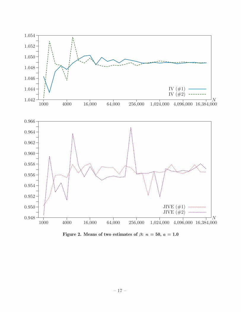
In the second experiment, a = 1.0, and the instruments are therefore a good dealstronger. As seen in Figure 2, the averages of the IV estimates now converge quicklyto a value of approximately 1.0489, which involves much less upward bias than before.The averages of the JIVE estimates do not seem to converge, but they vary muchless than they did in the first set of experiments, and it is clear that they tend tounderestimate β.

In additional experiments that are not reported here, we also tried a = 0.25 anda = 2. In the former case, the results were quite similar to those in Figure 1, exceptthat the upward bias of the IV estimator was much greater. In the latter case, wherethe instruments were quite strong, the averages of both the IV and JIVE estimatesappeared to converge, to roughly 1.012 for the former and 0.991 for the latter. Thus,based on the simulation results for this case, there was no sign that the JIVE estimatorlacks moments. It would presumably require very large values of N to illustrate thelack of moments when the instruments are strong.

7. Conclusions

In this paper, we have proposed a novel way to investigate the existence of momentsfor instrumental variables and related estimators in the linear regression model. Ourmethod is based on the use of polar coordinates. For generalized IV and K--classestimators, we obtain standard results in a new and simpler way. However, the mainresult of the paper concerns the estimator called JIVE. We show that this estimator hasno moments. Simulation results suggest that, when the instruments are sufficiently

– 14 –

weak, JIVE’s lack of moments is very evident. However, when the instruments arestrong, it may not be apparent.

References

Angrist J. D., G. W. Imbens, and A. B. Krueger (1999). “Jackknife instrumentalvariables estimation,” Journal of Applied Econometrics, 14, 57–67.

Anderson, T. W. (2003). An Introduction to Multivariate Statistical Analysis, ThirdEdition. Hoboken, NJ, John Wiley & Sons.

Blomquist, S., and M. Dahlberg (1999). “Small sample properties of LIML and jack-knife IV estimators: Experiments with weak instruments,” Journal of Applied

Econometrics, 14, 69–88.

Davidson, R., and J. G. MacKinnon (2004). Econometric Theory and Methods, NewYork, Oxford University Press.

Davidson, R., and J. G. MacKinnon (2006). “The case against JIVE,” Journal of

Applied Econometrics, 21, forthcoming.

Fuller, W. A. (1977). “Some properties of a modification of the limited informationestimator,” Econometrica, 45, 939–53.

Hahn, J., J. A. Hausman, and G. Kuersteiner (2004). “Estimation with weak instru-ments: Accuracy of higher order bias and MSE approximations,” Econometrics

Journal, 7, 272–306.

Kinal, T. W. (1980). “The existence of moments of k-class estimators,” Econometrica,48, 241–49.

Mariano, R. S. (2001). “Simultaneous equation model estimators: Statistical propertiesand practical implications,” Ch. 6 in A Companion to Econometric Theory, ed. B.Baltagi, Oxford, Blackwell Publishers, 122–43.

– 15 –

−3.0

−2.0

−1.0

0.0

1.0

2.0

3.0

4.0

5.0

6.0

1000 4000 16,000 64,000 256,000 1,024,000 4,096,000 16,384,000

................................................................................................................................................................................................................................................................................................................................................................................................................................................................................................................................................................................................................................................................................................................................................................................................................................................................................................................................................................................................................................................

.......................................................................................................... IV

...........................

........

...........................

..................................................................................................................................

......................................................................

...

...

...

...

...

...

...

...

...

...

...

...

...

...

...

...

...

.................................................................................

....................................

............... JIVE (#1)

..................................................................................................................

....................................................................................................................................................................................................................................................................................................................................................................

............................................................................................................................................................................................................................................................................

......................................................................................................................................................................................................

..............................................................................................................................

......................................................................................................

..........................................................................................................................................................................................................................................

...........................................................................................................................

.........................................................................................................................................................................................................

............................................................................ JIVE (#2)

N

Figure 1. Means of two estimates of β: n = 50, a = 0.5

– 16 –

1.042

1.044

1.046

1.048

1.050

1.052

1.054

1000 4000 16,000 64,000 256,000 1,024,000 4,096,000 16,384,000

........................................................................................................................................................................................................................................................................................................................................................

.....................................................

.............................................

.............................................................................................................................................

..........................................................................................................................................................................................

................................................................................................................................................................................................................................................................................................................................................................................................................................................................................................................................................

..........................................................................................................IV (#1)

..........

..........

..........

..........

..........

..........

..........

..........

..........

..........

..........

..........

..........

..........

..........

..........

..........

..........

..........

..........

..........

..........

..........

..........

..........

....................................................................................................................................................................................................................................................................................................................................................................................................................................................................................................................................................................

......................................................................................................................................................................................

..........................................................................................

..........................................................................................................................................................................................................................................................................................

................................................................................IV (#2)N

0.948

0.950

0.952

0.954

0.956

0.958

0.960

0.962

0.964

0.966

1000 4000 16,000 64,000 256,000 1,024,000 4,096,000 16,384,000

.........................................

......................

.......................

..........................

.............................................

...............................

.........................

...................

...............JIVE (#1)...................................................................................................................................................................................................................................................................................................................................................................................................................................

..........................................................................................................................

.........

........

.........

.........

.........

.........

.........

.........

.........

.........

.........

.........

.........

.........

.........

.........

.........

.........

.........

.........

.........

.........

.........

.........

.........

.........

.........

.........

.........

.........

......................................................................................................................................................................................................................................................................................................................................................

...........................................................................................

.........

...........................................................................................................................................................................................................................................................................................................................................................................................................................................................................

...........................................................................................................................................................................................................................................................................................................................................................................

..........................

......................................................

............................................................................JIVE (#2)N

Figure 2. Means of two estimates of β: n = 50, a = 1.0

– 17 –