Moments of Transition-Additive Random Variables Defined on

JOURNAL OF MATHEMATICAL PSYCHOLOGY 32, 313-340 (1988)

Moments of Transition-Additive Random Variables Defined on Finite, Regenerative Random Processes

RICHARD SHIFFRIN AND MAYNARD THOMPSON

Indiana University

Random processes consisting of a sequence of jumps from one to another of a finite set of states are considered. Such processes are regenerative if the progress after the nth jump depends only upon the state entered at the jump. Examples include discrete and continuous Markov processes. A method is given to restrict attention to a subset of sample paths according to criteria based on the transitions allowed for a single jump. The primary concern is with transition-additive random variables: these sum for any valid sample path the values of independent random variables assigned to each jump in the path. A simple formula for finding all moments of such random variables is derived. Necessary and sufficient conditions for the existence of the solutions are demonstrated, and illustrations of the computational simplicity of the approach are provided. ‘1 1988 Academz Press. Inc

I. INTRODUCTION AND OVERVIEW

In this paper we study a class of random variables defined on random, regenerative, finite-state processes. These include Markov and semi-Markov processes as special cases. A realization of the process is a path of jumps from one to another of the states of the process. The random variable under investigation sums values that are assigned to the jumps in a path. Our primary result is a theorem giving an elementary procedure for calculating all moments of such random variables. Examples and related questions have been investigated in many instances, both pure and applied’ (e.g., Barbour & Schassberger, 1981; Chung, 1967; Gibbon, 1971; Ginsberg, 1971; Glynn & Inglehart, 1986; Howard, 1971; Kao,

This research was supported, in part, by a grant to the first author, NIMH 12717. Reprint requests should be sent to Richard M. Shiffrin, Dept. of Psychology, Indiana University, Bloomington, IN 47405. The authors thank the reviewers for their careful and helpful comments.

’ The results presented here were reported at the Mathematical Psychology Meetings at Santa Barbara, California, in August, 1981, and at the IMACS Congress on Scientific Computation in Oslo, Norway, in August, 1985. A version of this paper was submitted to the Journal of Mathematical Psychology in January, 1983. Although that version was not accepted because it was too concise and lacked examples, the mathematical content was the same as that of the present version. We view the mathematical contribution as. significant for both the generality of the setting and the ease of implementing the computational algorithm. The paper contains a number of published results as special cases, including some that have appeared since our early submission. Our results not only are quite general but also contain ideas that are likely to be of special interest and usefulness to theorists in psychology.

313 0022-2496188 $3.00

Copyright 0 1988 by Academic Press, Inc. All rights of reproducrmn in any form reserved.

314 SHIFFRIN AND THOMPSON

1974; Kemeny & Snell, 1976; Millward, 1969; Neuts, 1976; Pike, 1966; Pollack & Arnold, 1975; Thompson, 1981). Special cases of these results, without proofs, have appeared in Shiffrin and Thompson (1986).

In psychology, Markov models have been used quite extensively (a few examples include Atkinson & Crothers, 1964; Bower & Theios, 1964; Brainerd, Desrochers, & Howe, 1981; Rapoport, Stein, & Burkheimer, 1979, Chap. 3, pp. 52-54). Most applications have involved discrete chains in which the time variable, if it is treated at all, is a function of the number of transitions. When the transitions between states are governed by distributions of time, the processes are usually termed “semi- Markov.” Such processes have not generally been used as models in psychology, although a few examples exist (e.g., Fisher & Goldstein, 1983; Townsend, 1976; Meyer, Yantis, Osman, & Smith, 1975).

We show in this article that calculation methods for semi-Markov processes are little different from those for Markov processes and both involve elementary operations (solutions of simultaneous linear equations). The methods presented are widely applicable and may make semi-Markov processes readily available to theorists in psychology and other fields. Even within discrete Markov chains, the methods provide a straightforward approach to the calculation of moments that might otherwise seem inordinately complex.

Although the theorems in question involve just two equations (actually two systems of simultaneous equations: see Eqs. (6) and (8)), we think an understanding of the approach and its applicability is best achieved by an orderly progression from simpler processes and uses to the more complex cases. This introduction will therefore be devoted to a somewhat simplified and informal presentation of the basic results, along with illustrative examples. The precise formulation and technical details are given in the following sections: In Section II are the definitions and notation; in Section III are the theorems and proofs. Section IV contains an algorithm useful for speeding calculations and contains some additional examples. Section V contains concluding remarks.

A. Discrete Markov Chains

Although calculation methods for discrete Markov chains have been well studied, our exposition is clarified by beginning with this case. In addition, the approach we suggest offers increased power and simplicity even in the discrete case.

Suppose there are N states. The process consists of a series of jumps (transitions) from one to another of these states. The sequence of jumps made is termed a path. The probability that the next jump occurs to state j given that the process is currently in state i is denoted by pii (usually given as a set of entries in an N x N matrix). This probability is independent of the trial number and of the sequence of jumps prior to the current state.

When at least one of the states (or a nonempty subset of the N states) can be entered but not exited (due to certain of the pii being zero), then the chain is said to have “absorbing” states. Our methods apply to chains whether or not they have absorbing states, but the methods apply only to sets of paths that have a definite

MOMENTS FOR MARKOV PROCESSES 315

1 2 76

= (Vii )

123 123 123 1000 2 I 000 I

I 2

3 101 3

= [PI)) = Clll 5v

,/-’

q

FIG. 1. A branching tree depicting the first three jumps of the Markov chain defined by the p. matrix at the upper left. Valid paths defined by the cil and e, matrices are given by solid connecting lines. Probabilities of jumps and of paths are given as shown. The values assigned to jumps are defined by the vy matrix and these are given in parentheses. The summed values along each path are given in parentheses at the termination of the third jump. The summed values for valid paths that have ended in the first three jumps are given in the trapezoidal boxes (along with the probabilities of those paths).

ending jump. To specify these, we define an indicator variable, eg, which is 1.0 if a jump from i to j ends a path, and 0.0 otherwise. We also might wish to consider only a subset of the remaining possible jumps. We therefore define an indicator variable cii which is 1.0 if a jump from i to j continues a path and is 0.0 otherwise (obviously eii and cii cannot both be 1.0). We are interested in all paths that consist of a sequence of continuing jumps followed by an ending jump. These are called valid paths. It should be noted that the cii and e, can be chosen at the discretion of the researcher, subject only to the constraint that cii and eV cannot both be 1.0 (examples will be given shortly).

The ideas are illustrated in Fig. 1. A three state Markov chain is under con- sideration. The transition probabilities are given in the upper left matrix (labeled (pij)) in the figure. The possible paths starting in state 2 that are three jumps long are depicted in the figure as branches in the tree. Each jump is labeled with the probability of that jump. At the termination of each path is given the probability of that three jump path. The matrices labeled (c,) and (eU) at the top of the figure give the continuing and ending jumps that define valid paths. Paths that are valid, or potentially valid, are connected by solid lines; invalid jumps are indicated by dashed lines, and all subsequent jumps in those paths are dashed as well. In addition, jumps in paths following any ending jump are dashed.

The solid horizontal lines indicate paths that have ended (validly at that point. The probability of each such valid path is given in the trapezoidal box. (The matrix labeled (uii) and the values given in parentheses will be discussed shortly).

480/32/3-8


The first task is to provide a method to calculate for each starting state i, the probability that the process will result in a valid path. This probability is termed g;. These are given by solving the following set of simultaneous linear equations (for i such that g,#O):

gi= i e,P,i+ 2 cl/Pijgj. .j= 1 j=l

This equation is similar to the well-known equation used to calculate the probabilities of absorbtion in particular states in an absorbing Markov chain. In words, it says that the probability of a valid path starting in i is a sum over the next steps that end a valid path at once (the first sum) and the next steps that continue a valid path (the second sum); if a continuing step occurs (say into state j), the probability of moving to that state must of course be multiplied by the probability that a valid path will result afterwards (g,).

Since, for certain starting states, g, may be zero (e.g., when state i cannot be left, and the jump from i to itself is not an ending jump: pii = 1.0; e, = 0), the equations we give apply only to states i for which g,#O. (Otherwise an indeterminacy results.) It can be concluded that gj # 0 if there exists a path with greater than zero probability connecting state i to at least one state k from which an ending transition can be made. These notions will be formalized in Section III, but it is always easy in practice to determine which gj equal zero.

Although the gi are of some interest in their own right, our primary goal is the determination of moments of certain random variables defined on valid sample paths. The idea is simple; each possible jump in a path is assigned a fixed value, termed uij when the jump is from state i to state j. We define a random variable Z, that is simply the sum of the values assigned to each jump in a valid path starting in state i, conditional upon the path being valid. It is the moments of Zi that are desired. This idea also is illustrated in Fig. 1. The matrix labeled (0,) at the top of the figure gives the values assigned to each jump. These values are given in parentheses next to each jump in the figure, and the accumulated values for each path are in parentheses at each path termination. Some values for Z, are those in the trapezoidal boxes at the end of valid paths.

The expected value of Zi can be obtained from the following set of simultaneous equations (for i such that g, # 0) (let pI = E[Zi 1 valid path]):

(2)

The idea here is related to that underlying Eq. (1). In words, the expected value starting in state i is a sum over valid next steps, multiplying the probability of that step by the sum of the value of that step and any expected future value to come after that step. Since all future paths might not be valid, the expected value of a continuing path must be multiplied by the probability of future validity: gj. Also, to gain a proper expectation, since the sum across all paths may have probability less


than one, the sum must be divided by gi. As is the case for Eq. (I), Eq. (2) applies only for those states i for which g,#O.

It is useful at this point to look at applications and examples. Consider how the cli and eV may be used. If paths terminating with the first entry in state k are of interest, the column k entries in the matrix (eti) can be set to 1.0, with others set to 0.0 (ejk = 1.0, i = 1, 2, . . . . N). If only paths ending with a jump from state i to state k are desired, then only the ejk entry is set to 1.0. If paths that do not go through state k are desired (see Chung, 1967, p. 45) then column k of the continuing matrix is set to 0.0 (C$ = 0, j= 1, . ..) N). These examples suffice to illustrate the general idea.

The value matrix can be used for many purposes. If all ud are set to 1.0, then 2 is a count of all steps taken. Setting only certain uii to 1.0 sums only those steps. For example, setting uii = 1.0 for j= 1, . . . . N counts each step away from state i. Of course if visits to certain states are worth more than others, or if certain jumps are worth more than others, then the uj, may be chosen to reflect those values (as illustrated in the examples).’

EXAMPLE 1. Our first example is based on the Markov chain defined by the pq matrix in Fig. 1. To calculate the probability of a valid path, the use of Eq. (1) gives

g, = Ok,

g, = 0.5g, + osg,

g,=O.l +0.6+0.3g2.

Solving, g, = 21155; g, = 7/l 1; g, = 49155. To calculate the expected number of steps in a valid path, replace the value

matrix in Fig. 1 with a matrix filled with ones. Then Eq. (2) leads to

it =; W%,U +P~H

p,=; {WtU +h)+wAl +cc3G

p3=i (0.1 +0.6+0.3g,(l +P~)}.

Substituting the values of g, and then solving give pi = 51/11; p2 =40/11; ,uj = 137177.

’ It is probably good form to set e,, and c,, to zero when pe = 0, and to set u,, to zero when both e, = 0 and c,, = 0. However, since these terms multiply each other in the equations, it is unnecessary to do so. It may even prove convenient when exploring different sets of restrictions and values on a given chain to leave certain of these cells filled with nonzero values. The only necessary constraint is that 0 c c,, + e,, < 1.


For the value matrix of Fig. 1, Eq. (2) gives

Substituting for the gi and solving, pcLI z 27.70; pL2 123.70, ~1~ g 10.84.

Consider next the calculation of higher moments of Zi. The idea is the same as that in Eq. (2), except that in this case the appropriate formula is

1

wp; + i cijP~gjEC(v, + zjIpl}. j=l

Letting E[Zp] =#‘, Eq. (3) can be rewritten

(3)

(4)

Once again, these equations apply only to those states i for which gi#O. To solve for the pth moment, one solves the simultaneous equations for the first moments, substitutes the values obtained into the simultaneous equations for the second moments, and so forth. In each case, a set of N (or fewer) simultaneous linear equations needs to be solved.3

EXAMPLE 2. To illustrate the solution method, we use an example that keeps the calculations fairly simple: a five state random walk with two absorbing barriers (see Kemeny & Snell, 1976, p. 27).

The probabilities (pq) are given by a transition matrix,

1 0 0 0 0 iO$OO

(pv)= I 0 f 0 3 0 1 *

0 f f 0 0

00001

3 Actually, things are even easier than this. The solution of a set of simultaneous equations is equivalent to the inversion of a certain matrix. It turns out that the same inverted matrix can be used to solve for all moments and all value matrices, as shown in Section IV.


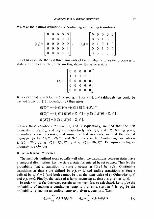
We take the natural definitions of continuing and ending transitions:

(e+~;;;;], ;;f~X].

Let us calculate the first three moments of the number of times the process is in state 2 prior to absorbtion. To do this, define the value matrix

0

1

0 . 0 0 /

It is clear that gi = 0 for i = 1, 5 and gi = 1 for i = 2, 3,4 (although this could be derived from Eq. (1)). Equation (3) then gives

Solving these equations for p = 1,2, and 3 sequentially, we find that the first moments of Z,, Z,, and Z, are respectively 715, 315, and l/5. Setting p = 2, expanding where necessary, and using the first moments, we find the second moments to be 63/25, 27/25, and 9/25, respectively. Continuing, we obtain E[Zz] = 763/125, E[Z:] = 327/125, and E[Zj J = 109/125. Extensions to higher moments are obvious.

B. Semi-Markov Processes

The methods outlined work equally well when the transitions between states have a temporal distribution. Let the time a state i is entered be set to zero. Then let the probability that a transition to state j occurs in [0, r] be p&t). Continuing transitions at time I are defined by c,(t) = 1, and ending transitions at time t defined by e&t) = 1 (and both cannot be 1 at the same value of t). Otherwise e,(t) and c&t) = 0. Finally, the value of a jump occurring at time t is given as vu(t).

In order to use the theorems, certain terms must first be calculated. Let qcij be the probability of making a continuing jump to J’ given a start in i; let qeg be the probability of making an ending jump to j given a start in i. Then

4cij = Jorn c,-(t) dP,W> s.,=J- e,(t) dpij(t), (5) 0


assuming that the integrals exist. (In (5), dpJt) refers to Lebesgue-Stieltjes integration. In many applications dpJt) may be replaced by p;(t) dt, that is, by the density function: see Example 3 and Fig. 2.) It is then possible to solve for the gi as in Eq. (l),

gi= f 4eik+ f qrik gk 3

k=l k-l

for states i such that g,#O. Next, let rc”i, be the pth moment of the value of a continuing jump from i to j, and z$ be the pth moment of the value of an ending jump from i to j, when qcii#O and qeij#O:

1

(7A)

(7B)

FIG. 2. An example of the use of the equations for semi-Markov processes. (See the discussion of the Land of Oz example in the text.) The chain, the valid paths, and the value functions are defined by the Lj(t), cV(z), e,(t), and u,(t) matrices. The various state to state jump probabilities that must be calculated in order to use the equations in the text are given in the lower portion of the figure, as are the weighted values assigned to those these jumps.


Moments can then be calculated using an equation essentially identical to Eq. (4):

As usual, these equations hold for states i for which g, # 0. Note that the basic formulas (Eqs. (1) and (4)) remain essentially unchanged in

the setting of semi-Markov processes. The computations will be more complex only because certain integrals (Eqs. (5) and (7)) must be evaluated before the basic equations (Eqs. (6) and (8)) can be used. The integrals involved in Eqs. (5) and (7) can be evaluated numerically.

The roles played by the matrices (c,(t)), (e,(t)), and (o,(t)) remain the same as those in the discrete case, although the entries in the matrices are now functions of time. Most often, c,(t) and e,(t) will be set equal to 0.0, or 1.0, over certain intervals of time (for ti). If, for instance, c,(t) = 0 within such an interval, then no valid path can have a jump from state i to state j within that interval. Likewise, if e,(r) = 1 in an interval, then any valid path jumping from state i to state j within that interval ends with that jump. Note in particular that it is possible for a transition from i to j to be continuing for some values of t an ending for other values.

The uses of the v,(t) matrix are also straightforward. Perhaps the most common usage in the semi-Markov domain will involve setting u,(t) = t for all i, j, and t. Then the random variable gives the cumulative time of travel in a valid path. Obviously many other options are available. For example, the time spent only in certain states can be counted by setting u,(t) = t only for those states i in question. Setting uii( t) = 1 will count number of transitions, as in the discrete case; setting zlli(t) = 1 only in certain time intervals will count number of transitions made in those time intervals. Thus if for all i, j, u,(t) = 0 for t < to, and u,(t) = 1 for t > to, then the random variable counts number of transitions in a valid path that take longer than to. Finally, note that the u,(t) assignments need not be restricted to 1 and 0, or to t: any values called for by the setting of the problem may be used. For example, if a system has the property that an output occurs from state k once state k is resided in for at least to set, and the output is proportional to the square root of the additional residence time beyond to, then the output value could be obtained by setting ukj(t) = 0 for t < to and uk,(t) = a(t - to)“’ for t > to, for some constant a, and all states j.

EXAMPLE 3. We use a version of the Land of Oz example of Kemeny and Snell (1976, p. 29) to illustrate the application of the method to continuous processes. Suppose that the weather in Oz changes randomly from moment to moment, among snow (S), nice (N), and rain (R), according to the matrix (f&t)) of densities given in Fig. 2. In words, this matrix says that the probability density of a transition (somewhere) from a state is decreasing exponentially so that the cumulative probability of a transition by time t is P, - P, exp{ ---air}, where 1 -P, is clearly the


probability that no transition will ever be made. If a transition is made, bi gives the conditional probability that it will be made to the first of the remaining two states (ordered R, N, S). For this example, we set P, =0.9, uR= 1, bR =0.4, P, =0.8, aN = 0.5, b, = 0.2, Ps = 0.7, as = 0.4, b, = 0.7.

Now suppose we wish to calculate the moments of the variable which sums up time as follows: it counts the total time spent in going from rainy to snowy weather, and from snowy to nice weather. It also counts the time going from rainy to nice weather, unless this time for any one such transition happens to be less than 1 day, in which case it counts a full day, or happens to be between 3 and 4 days, in which case it counts nothing, or happens to be greater than 4 days, in which case it counts 3 days.

We will consider only continuing weather transitions in which rainy to nice transitions take less than 4 days, rainy to snowy transitions take more than 2 days, nice to rainy transitions and snowy to nice transitions of any sort occur, and snowy to rainy transitions take less than 2 days. Finally, we will stop counting whenever a nice to snowy transition occurs, or when a rainy to nice transition takes more than 4 days, or when a rainy to snowy transition takes less than 1 day or when a snowy to rainy transition takes more than 2 days.

These assumptions are embodied in the (u,(t)), (c,(t)), and (e,(t)) matrices of Fig. 2. To apply Eqs. (6) and (8), we must find the various q’s and z’s for single jumps, and the results of these calculations are shown in the lower portion of Fig. 2. From Eq. (6) we have g, = qeRN + qrRS + qcRN gN + qcRS gS, gS = q&R + qrSR t?R +

q&N gN, gN = qCNs -t q&R g,, and COnSequentiy (using the Values for the q’s) .g, = 0.552, g, = 0.744, g, = 0.651. Next we use Eq. (8) to obtain

1 pi =- qeRNT:RN + qeRSr:RS + qcRN gN

p--m CRN PN

gR

+qcRSgS f m=O (3 7:RSPg-“)

1 &=-

gs qcSR@gR+qcSNgN i ,_,(3 r%N@-m]

Solving for the first moments only, one finds ps = 1.08, ,!+, =0.146, and p(R = 1.04. The higher moments may be determined iteratively.

In this section we have given an informal exposition of the results in a slightly restricted setting and have given examples. The discussion in the following section introduces a somewhat more general setting in which “time” is replaced by a variable in a more general parameter space, perhaps multidimensional. It is in this more general setting that we make the concepts and methods precise and that we prove the theorems (in Section III).


II. DEFINITIONS AND NOTATION

We introduce a setting which is general enough to emphasize the wide applicability of the results. Consider a random process, taking values in a finite state space S= { 1, 2, . . . . N}, which jumps from state to state with probabilities depending on the states and on a parameter in a parameter space Y-. More specifically, suppose that we have an Nx N matrix of real-valued set functions defined4 on a a-algebra % in F with the properties

&j(A)30 for each A E %, i, j = 1, 2, . . . . N

c P&m G 1, i= 1, 2, . . . . N

and

for each countable collection

of nonoverlapping sets A, in

42, i, j= 1, 2, . . . . N.

For i, jES and a set f3~%, a set of jumps (or transitions) from state i to j with parameter in 8 will be denoted (i, 8, j) and we introduce a probability measure P, conditioned on the starting state, by

PC(i, 8, j) I il = hp).

In words, conditioned upon the starting state being i, pJ8) gives the joint probability that a jump is made to j and that the parameter will take a value in 8. For each t E 6’ we write (i, t, j) as that element of (i, 8, j) with parameter t. In the jump (i, t, j) we refer to i as the beginning state and j as the ending state. A sample path is a sequence of jumps with the beginning state of the (n + 1)st jump coinciding with the ending state of the nth jump. A sample path y can be denoted by

where k,,, k, E S, t, E Y for m = 1, 2, . . . . The set of sample paths beginning in state k, and passing (in order) through the states k,, k,, . . . . and with t, in a set 8, E % for m = 1, 2, . . . . will be denoted by IY Equivalently r= ((k,, 01, k,, 8,, k,, . ..)}. Note that the case k,,- i = k, is not excluded. The transition (k,- i, t,, k,) will be referred to as the nth jump and t, as the parameter for this jump. The probability of the set of sample paths r is defined to be

w-i = n ~km-lkmvu ma1

4 A o-algebra is a collection of subsets which is closed under countable union and complementation. Such a class of subsets provides the appropriate setting for the study of probabilistic problems of the type considered here (and almost all others).


This construction guarantees the regenerative character of our process: there is a probability p,(e) of entering j from i with parameter value in the set 6 which is independent of the initial part of the sample path. In particular, this probability is independent of when in the sequence of states i is entered.

In the special case when F = R+ = {x E R. .x > 0 > and the sets 0 are intervals [0, t] we use the notation p&t) instead of p,(8). In this case we define p&t) to be the conditional probability that if there is a jump into state i at t = 0, then the next jump is into state j and it takes place in the interval (0, t].

Note that we allow for the possibility that for some states i,

N

1 p&Y-)< 1. ,=I

When F is time, we may interpret such a defective case by saying that the process may reach some state and with positive probability never make another jump. This

(b= (km t,, k,, t,, k,, . ..t k.v-1, t,, k,). (*I

segment 4 of the form (*) will be said to be of length s. Let C (continuing) and E (ending) be disjoint sets of jumps with indicator

functions

1 if (i, t, j) E C 1 c,(t) =

if (i, t, j) E E 0 otherwise ’ e,(f) = 0 otherwise ’

illustrated in one of the versions of Example 4 in Section IV. Initial segments of sample paths will be denoted by

i, j= 1, 2, . . . . N, t E 5. Define di, i= 1, 2, . . . . N, to be the set of all finite initial segments of sample paths of the form (*) with s b 1 and

k,=i,

(kj-1, tj,kj)EC, j= 1,2, . . . . s- 1,

(k,-,, t,,k,)~E.

(These concepts are related to the taboo states of Chung [ 1967, Sect. 1.91). To facilitate our discussion it will be convenient to use dti to represent a jump

(i, t, j) E C, and dj to represent a segment (j, ti, k,, . . . . t,, k,) E Aj. With this notation we define bjj+ $j to be the segment 4 E Ai:

4 = (i, t, j, t,, k,, . . . . fs, k,).

Thus the symbol + in 4ii + #j indicates the concatenation of dii and 4j. We write (k,, t, k2) E 4 to mean that there is a jump (k,, t, k,) somewhere in the segment 4. With this notation the following assertion is obvious.


Every 4 E Ai is exactly one of:

(a) a single jump, in which case I$ E E, or

(b) a sequence of two or more jumps, in which case it can be written as dii + 4, with d,, E C and dj E A,.

Let (v,(t)) be an N x N matrix of finite real valued functions defined on Y. Define a random variable Z, on Aj by setting

Z,(9) = f; Uk,-,k,@,) ., = 1

for 4 E Ai of length s. Since Zi is a sum of values associated with one step jumps or transitions, we refer to such random variables as transition-additive.

In what follows it will be useful to have notation for specifying the value assigned to a single jump, continuing or ending. To this end

forf$=(i,t,k)EC set Tci!f(d) = oik(f)

and

ford=(i, t,k)EE set Ted141 = ~dt).

Finally, we need notation for the probabilities of certain sets of valid sample paths or segments of such paths. For a given state i, let gi be the probability of the set of valid sample paths starting in state i where the universal set is all sample paths starting in state i. Similarly, for i, Jo S set

That is, qcii is the probability of making a continuing jump to state j given a start in state i, and qcli is the probability of making an ending jump to state j given a start in state i.

Our interest is in the moments of the random variable Zi, and we next introduce notation for these moments. For i, Jo S and p = 1, 2, . . . . we set

These moments are conditional so that the expectations are proper, which leads to a convenient and easily understood formula for the calculation of the moments. To be precise, note that


when qCv # 0 and qei/ # 0. The states i for which gi > 0 can be determined by forming an (N + 1) x (N + 1)

matrix W with

1 if q,,>O, i= 1, . . . . N;j= 1, . . . . N N

1 if C qeik>O, i= 1, . . . . N;j=N+ 1 h,= k=l

1 if i=N+ l;j=N+ 1

0 otherwise

and computing W N. Any state i for which the (i, N + 1) element of W N is positive has g,>O (see Kemeny & Snell, 1976, Chap. 2).

In what follows we suppose that the probabilities gi, qCii, and qeii exist, an assumption which imposes mild restrictions on the applicability of the results. Since the sets C and E are determined by specifying the class of admissible sample paths, the existence of qCi/ and qeii depends upon the relations between the constraints of admissibility (the cu and eU) and the measure pii.

III. DETERMINATION OF THE MOMENTS

Our primary goal (Theorem 1) is to derive a formula for the pth moments of transition-additive random variables. This result is supplemented by an existence theorem (Theorem 2) which shows that if the one step moments exist, then moments for valid paths of arbitrary length do also, and by a theorem (Theorem 3) which shows that the formula of Theorem 1 can be used to determine the pth moments recursively. The notation used in the statements of the theorems was introduced in Section 2, and readers interested primarily in applications will find the statements of Theorems 1, 3, and 4 self-contained. We emphasize that all probabilities in this section are understood to be conditioned on the path starting in a particular state, which we refer to as i.

THEOREM 1. For those i with gi > 0 and any p for which the moments exist,


Remarks. (i) It is suggestive to write the formula of Theorem 1 in the form

This formulation emphasizes the basic idea of viewing each sample path as a first step followed by a (possibly missing) subsequent.

(ii) The special case of this result for first entrance times conditioned on the avoidance of specified states appears in Chung (1967, p. 62).

(iii) The probabilities g, can be obtained by using a well-known relation involving absorption probabilities in discrete Markov chains. The details are provided in Theorem 4.

Proof of Theorem 1. Partition the set di into N+ 1 subsets: one consisting of Ai n E, and N other subsets of A,, each consisting of sample segments of length greater than 1 whose first transition is to a specific state. Each sample path in one of these N latter subsets can be written as 4 = 4jk + dk, 4ik E C, dk E A,. It may be that one or more of these subsets is empty.

On Ai the random variable 2; is a probabilistic mixture of N+ 1 random variables, namely Zi restricted to each subset of Ai, each weighted according to the probability of the appropriate subset. It follows that CL/ can be written as a sum of the weighted expectations of the restrictions of Zp, where a weight is the probability of the appropriate subset:

k=l

=i i kg, qeikECTeq.k I dik EEI

+,f,, qrrkgkE[(Tcik+Zk)PI~ikEC,~kEAkl .

The formula of Theorem 1 is obtained by expanding the last term on the right hand side in the expression for @ above and noting that Trik and Zk are independent. 1

The hypothesis of Theorem 1 that the moments,plp exist can be replaced by the (apparently simpler) assumption that the one step moments exist. This is the content of the next result.

THEOREM 2. Zf the probabilities gi, qCik, q& k E S, and the moments ztik, &, k E S, and h = 1, 2, . . . . p exist, then the moments of Zi of order up to and including p also exist.


We begin by showing that there is a discrete absorbing Markov chain for which the first passage time distribution is closely related to our process.

LEMMA 1. There is a discrete absorbing Markov chain with one absorbing state and n (d N) transient states with the following property: if Sj is a random variable defined on the discrete chain which assigns to each sample path starting in state i the number of transitions to absorption, and zf A; is the subset of Ai which contains sample paths with exactly s jumps (s - 1 continuing and 1 ending), then

for iES with g,>O and s= 1, 2, . . . .

Proof Introduce as transient states all states r E S for which g, > 0. Without loss of generality we suppose these states to be numbered 1,2, . . . . n. Form an (n + 1) x (n + 1) transition matrix for a discrete Markov chain as

j= 1, 2, . . . . n; r = 1, 2, ,.., n

j=n+l;r=l,2,...,n

i 0,

P n+l.j= 1,

j = 1, 2, . . . . n

j=n+l.

Since the row sums are 1, this clearly defines a legitimate transition matrix. Also, for each r, since g, > 0, there is a positive probability of reaching state n + 1 in n steps. Thus we have an absorbing Markov chain. Note that in essence the absorbing state has been obtained by collecting all ending jumps together.

Next, fix k, , kZ, . . . . k,_ 1 and consider the set of all sample segments which begin in state i, are of length s (consist of s jumps), and pass successively through k,, k,, . . . . k,- I and end in state k,. Denote this set by A;(k,, kZ, . . . . k,). Letting i= k,, it follows that

P G Af(k k,= 1

1,...,k,)/Ai =iP 6 Ay(k,,...,k,) 1 I [,..I 1

=$ ;c’ qck,-,k, i qek,-,m, (9) ‘I 1 ??I=1


and that

= +- I!’ qck,e,k, f q&m ,m. (10)

‘I 1 m=I

Here (9) applies to the original process and (10) to the discrete analogue, and since the right hand sides are equal, the left hand sides must be equal also. Thus the probabilities of each subset of sample paths for the processes are equal. Also, the possible sets of intermediate states are identical, and the conclusion of the lemma follows. 1

LEMMA 2. For i = 1,2, . . . . n and each p, E[Sp] < co.

Proof. For states i, j in the discrete chain, let p&m) denote the probability of going from i to j in m steps. There are (Kemeny & Snell, 1976, p. 43) numbers b > 0 and 0 < c < 1 such that p@(m) < bc” for any transient states i and j. Consequendy, the probability that the process begins in state i and reaches the absorbing state in exactly s steps satisfies

Therefore

ig, pii(s- 1) pj,n+l <nbc’+‘, s= 1, 2, 3, . . . .

E[Sp]= f sPP[S,=s}6nb f spcs-‘, s=l .s= I

which is clearly finite. 1

Proof of Theorem 2. With A; as defined in Lemma 1, decompose Ai into disjoint subsets Af so that Ai = lJsa 1 A;. Using this decomposition we have

P[Zi$.~A,]=;P[Zi<u] I

Next,

= 1 P[+:Z,(i)<ul~~A;(k ,,..., k,)] P[&~d;(k ,,..., k,)[d~A;]. (12) ki. . . . . k, all Daths

SHIFFRIN AND THOMPSON

where there are at most p moments in the product on the right with nonzero order. Thus, if M 2 1 is a bound for E[ Tk] for all 7’s and k = 1, . . . . p, then the right hand side of Eq. (13) is no larger than

Using Eq. (12), Eq. (13), and the estimate Eq. (14),

The proof is now completed by using this estimate and Eq. (ll),

which is finite by Lemmas 1 and 2.5 1

(14)

5 The idea behind the proof of Lemma 2 and Theorem 2 can be used to obtain the following result for random sums. Let S be a finite set of random variables, each of which has finite moments of orders up to and including p, and let N be an integer valued random variable with finite moments of all orders. Define a random variable T = T, + T, + . + TN where each Ti E S. Then T has finite moments of order up to and including p.

MOMENTSFOR MARKOVPROCESSES 331

We turn next to the use of the formula of Theorem 1. In order to determine the moments one first calculates the probabilities gi (see Theorem 4 below), then pLf, iE S, then p’, in S, and so forth. For each p, the determination of p;, iE S, requires the solution of no more than N simultaneous linear equations. The fact that these equations are always solvable is the content of the next result.

THEOREM 3. If the probabilities g;, qrjk, qrik, i, k E S, and the moments z$, &, i, k E S, h = 1, 2, . . . . p, exist, then the equations of Theorem 1 can be solved recursively to yie/du:, iES, h=1,2 ,..., p.

Proof Suppose that the states are labeled as in Lemma 1; i.e., states 1, 2, . . . . n (n G N) have g, > 0. For p 3 1 suppose that the moments pf, iE S, h = 1,2, . . . . p - 1, have been determined and that the one step moments of order p exist. From Theorem 1 we have

i = 1, 2, . . . . n. Denote by a,(p) the right hand side of Eq. (15) and by a(p) the n-vector whose ith coordinate is ai( Under the hypotheses of the theorem, a(p) contains only known quantities. Also, let m(p) be an n-vector whose ith coordinate is pp. Then Eq. (15) can be written as

where 0 is the n x n identity matrix and Q is the portion of the transition matrix introduced in Lemma 2 which involves transitions between transient states; Q = (( l/gi) qCiigj). Since I - Q is invertible (Kemeny & Snell, 1976), Eq. (15) can be solved. If (0 - Q)-’ = N (the fundamental matrix for the absorbing Markov chain of Lemma l), then we have

m(p) = fWp). I (16)

In order to establish the formula for the probabilities of a valid path given a starting state, we need the following lemma.

LEMMA 3. There is a discrete absorbing Markov chain with two absorbing states and n 6 N transient states with the following property: P[A, 1 i] = P~,~+, , where p,,“+, is the probability of absorption in the first of the two absorbing states of the discrete chain.

Proof: Introduce as transient states all states r E S for which g,> 0. Without loss of generality we suppose these states to be numbered 1, 2, . . . . n. The transition

48013213.9

332 SHIFFRIN. AND THOMPSON

probabilities between these states are the qcii. The first absorbing state corresponds to having made an ending transition and the second to never making a transition at all. More precisely, we form an (n + 2) x (n + 2) transition matrix for a discrete chain as

r= 1, 2, . . . . n;j= 1, 2, . . . . n

r=l,2,...,n;j=n+l

1 - i (qcrk + qerkh r = 1, 2, . . . . n;j=n+2 k=l

i

0, P

j = 1, 2, . ..) n;j=n+2 n+l,j=

1, j=n+l

0, Pn+Li= 1 L

j= 1, 2, . ..) n + 1 j=n+2.

The row sums are clearly one, so this defines a legitimate transition matrix. Using the terminology of Lemma 1, it is obvious that

P L

(j A;(k s- I

I 2 ...Y ks) = n qck,-,k, k,= I 1 j= 1

f, qeks-,m

which is the probability of a path in Ai of length s through intermediate states k,, kZ, . . . . The right hand side of this equation is the probability of the corresponding path for the discrete chain. The correspondence holds for all sample paths of all lengths, and Ai= lJS A;, so the conclusion of the lemma follows. 1

Theorem 4 now follows directly from the standard result for absorption probabilities in finite chains (Kemeny & Snell 1976) and provides a means of computing the probabilities g,.

THEOREM 4.

gi= f qeik+ 2 qrikgkr iES, g,>O. k=l k=l

Remarks. (i) The case of a jump from a state to itself is permitted in order to include the possibility that the process spontaneously “forgets” and the parameter values are “reset” even though there is no change in state. Also, the option of having a jump from a state to itself may be useful to theorists in cases where jumps are observable events. Of course such transitions can be excluded if they present difficulties in the design or interpretation of experiments.

(ii) Without loss of generality, c&t) and e,(t) may take on values between zero and one, whose sum is less than or equal to one. In this case, the values may be given probabilistic interpretations. We illustrate in Example 5 in the next section.

MOMENTSFORMARKOVPROCESSES 333

(iii) Without 1 oss of generality, the fixed value o,(t) may be replaced by a distribution of values. In such a case, Theorem 1 and Eq. (8) are correct as given, but Eqs. (7A) and (7B) must be modified so as to obtain the correct expectation. Also the versions of these equations contained in Eqs. (3) and (4) would require replacement of the terms 06 with E[t$].

(iv) The proofs of the theorems in a context in which time has been replaced by a point in an arbitrary parameter space allows for some potentially useful processes. For example, a multistate process could be defined over both time and space; in this case the parameter of the process for each state would be a point in a four dimensional space.

IV. AN ALGORITHM FOR CALCULATING MOMENTS AND EXAMPLES

In Section III we developed a matrix formulation of our results. This formulation provides a convenient way to give an explicit method for determining the moments recursively.

ALGORITHM FOR CALCULATING MOMENTS

1. Determine the matrices (p,), (c,), (e,), and (vii). (In general these matrices will depend on choices made by the theorist.)

2. Compute the probabilities (qcti) and (qeij) using the definitions

and the probabilities gj (for those i for which g; > 0) using the equation

g,= f qelJ+ % 4rq gj. /=I j= 1

3. Compute the one step moments using the equations

5. Following the development of Section III, suppose that the states numbered 1 through n are those with g; > 0, and the states numbered n + 1 through N each have gi= 0 although they may have valid sample paths ending there with positive probability. Define an n x n matrix Q by setting Q = [(l/g,) qciigj] and


set fV = (0 - Q)-‘. Let m(p) be an n-vector whose ith coordinate is @, and let r(p) be an n-vector whose ith coordinate is

Also, let TLp) be the n x n matrix (r$), and let Mlcp) be the n x n matrix whose diagonal entries are those of m(p) and whose off diagonal entries are 0. Set M(O) = 0.

Finally, for n x n matrices A and B define A * IE! to be an n-vector whose ith coordinate is C,“=, agbg. With this notation the formula for determining the moments recursively is

Formula (17) holds under the conditions of Theorem 3.

Note that the matrix fV in formula (17) is independent of the value matrix (vii(t)). Consequently, all moments of any transition additive random variable can be determined with the same matrix fK (for given matrices (c~) and (eV)).

This algorithm is easily translated into computer code, and it provides a very efficient method of determining moments. We illustrate the simplicity and efficiency of the method with two additional examples.

EXAMPLE 4. Using the results of this section and Eq. (17), we calculate again the first three moments of the random variable defined in Example 2:

cl+ d g, N=[i ! I]

r(m)= [%I, Tym)= [i A KJ, m=l,2,3.

From this it follows that

m(l)= N. [[g+[$[g

m(2)= N. [[y+[;]+2[g]=[$


and

m(3)= N . [[~]+[~]+3[~]+3[3]~[3.

One of the advantages of this method is that the task of computing moments for several random variables with the same conditions (same (pti), (cii), (eV)) is simplified. For instance, we can construct another version of this example by defining a random variable as follows: count a visit to state 2 as of vaIue 1, a visit to state 3 as a value of -2, and a visit to state 4 as of value 5 if the next state is 5 and 0 otherwise. We have

0 0 0 0 0

1 1 1 1 1

0 0 0 0 5

0 0 0 0 0

1 1 1 (-2)” (-2)” (-2)” )

I m = 1, 2, 3.

0 0 0

Consequently

m(l)=N [ [$]+.[-g=[$

m(2) = N [[iJ+[;]+2[-;]]+J

and

m(3)=N[[l]+ [;:I+3 [-!]+3[li]]=[$].

As a final version of this example, suppose that the second version is modified so that the only ending transitions are those into state 5. State 1 is still an absorbing

That is, g, =A, g, = :, g,= g. We determine the first moments of the random variable defined in the second version. We have N, (u,), and TUT”) as in that version and

0 r(m) = [ 1 0 7 m = 1, 2, 3.

(5y+ ‘/I

Consequently

r 1.390 1 m(l)= [:St; J, m(2)= [ ,kif], m(3)= [ ‘%!iEI].

It is worthwhile to reiterate a point made earlier: the c&t) and e,(t) need not be indicator variables. Rather, they may be arbitrary (measurable) functions with values between 0 and 1 subject to c,(t) + e&t) < 1. In such cases the values may be interpreted as probabilities. For example, if c&t) = 0.5 for all t, then the probability that a jump from state i to state j at time t will be continuing is 0.5. None of our equations are altered by this change. We illustrate with an example.


state, but sample paths which terminate in state 1 are not in A,, i = 2, 3, 4. Then g,, g,, g, are determined from the system

g2 = 3 g3

g3 = i g2 + s g4

g,=j+fg,.

EXAMPLE 5. Consider a three compartment stochastic system which we model in terms of a semi-Markov process. Suppose the holding times for transition from states 1 and 2 are exponentially distributed with parameters 1 and 0.5, respectively, and suppose transitions from state 3 occur 1 time unit after it is entered. We assume that the matrix of distribution functions is

where

[

0 0.4(1-e-‘) 0.6(1-e-‘) (pg)= 0.2(1 -ePO.“) 0 0.8( 1 -e-O.“) ,

0.7h(t) 0.3h( t) 0 1 0

h(t)= 1 1

for t<l for t31’

Also, suppose that valid sample paths are defined by continuing and ending transitions specified as follows: Let T denote holding time. Continuing transitions are those


- from state 2 to state 1

- from state 1 to state 2 with T < 4

- from state 1 to state 3 with T> 2

and ending transitions are those

- from state 2 to state 3

- from state 1 to state 2 with Ta4

- from state 1 to state 3 with T-c 1.

Finally, transitions from state 3 to states 1 and 2 are continuing with probability 0.5 and ending with probability 0.5. (Transitions from state 1 to state 3 with 1 d T< 2 are not valid.)

The random variable we consider is defined as follows:

- to transitions from states 1 and 2 to state 3 assign the holding time T,

- to transitions from state 1 to state 2 assign the integral part of T for T< 4 and assign the number 4 for T> 4,

- to transitions from state 3 to state 1 assign the number 1, - to transitions from state 3 to state 2 assign the number 0.

These assumptions can be summarized as

0, T-c4 l,T<l

1, Tk4 I 1 O,T>l


Applying our results, we begin by determining g;, qcii, and qey for i, j = 1,2, 3. The nonzero q's are qEIZ =0.3927, qc13 = 0.0812, qc2, =0.2000, qrjl =0.3500, qr32 = 0.1500, qe12 =0.0073, qe13 =0.3793, qe23 =0.8000, qp31 =0.3500, qe32 = 0.1500. Solving the system of equations of Theorem 4 for the gi we have g, = 0.8434, g, =0.9687, g, =0.9405.

We determine the one step moments of our random variable by using Theorem 1. We have, for p = 1,

5<,2 = 0.5073, 2(.13 = 3, t,.3, = 1, t,i2 = 4,

~~~~ = 0.4180, T~23 - -2, z,31= 1,

and for p = 2,

r;,2 =0.8740, ~~~~ = 10, Sf3* = 1, T:,, = 16,

T:,, = 0.2541, 2;23 = 8 > zz31 = 1.

We now have the data necessary to determine the first two moments of 2,) Z2, and Z,. Using the formula of Theorem 1 with p = 1 we find

p1 = 1.722, p2 = 1.951, /LLj = 1.311.

Now that we have the first moments, we can use the formula of Theorem 1 again, this time with p = 2, to determine the second moments. We find

p(: = 7.175, ,u;= 7.856, p;= 5.233.

The technique is clear, and we could determine the moments of the random variables Z,, Zz, Z, of any specified order by repeatedly applying Theorem 1. Alternately, we could calculate the moments by using Eq. (17), which is essentially a matrix version of the formula of Theorem 1.

V. CONCLUDING REMARKS

Our goal in this article has not been to apply the techniques developed here to particular problems in the psychological arena, nor have we done so. We feel that specific applications might detract from the generality and simplicity of the approach: Computations for the examples given in the article, and for the moments of any transition-additive random variable, are based on just two equations, Eqs. (6) and (8 j, which form the content of Theorems 1 and 4.

From the standpoint of applications in psychology, we anticipate that in some situations the efficiency of the method will be of most interest. In other cases, the flexibility of defining valid sample paths or repeating the calculations easily for several random variables may be most important. However, it may well be that the greatest use will be in the calculation of moments for semi-Markov processes. This


class of processes has not been widely used, and perhaps the technical tools of this article will encourage geater use.

Finally, we remark that transition-additive random variables SU~M values assigned to each jump in a valid path, and there are other interesting and potentially useful random variables such as one that multiplies the values assigned to each jump in a valid path. Equations similar to Eqs. (6) and (8) can be used in such cases (and more complicated ones) but it is difficult to specify conditions under which the solutions will make sense, and under which the moments will exist. However, one such case can be handled using the present results. Suppose 2’; is a random variable giving the producr of values (u,(t)) along a valid path (u,(~)>O). Define a new value matrix (v:(t)) such that u;(t) = log o,(t). Define a new random variable Zj that sum the values of u* along a valid path. Our present methods give the moments of Zi. Since Zi = log X,, one can infer characteristics of the distribution of Xi from the moments of Zi. Note, however, that although the moments of Z, may exist, the moments of Xi may not.

REFERENCES

ATKINSON, R. C., & CROTHERS, E. J. (1964). A comparison of paired associate learning models having different acquisition and retention axioms. JournuI of Muthematicul Psychology, 1, 285-315.

BARBOUR, A. D. & SCHASSBERGER, R. (1981). insensitive average residence times in generalized semi- Markov processes. Advances in Applied Probability, 13, 720-735.

BOWER, G. H., & THEIOS, J. (1964). A learning model for discrete performance levels. In R. C. Atkinson (Ed.), Studies in mathematical psychology (pp. 32-94) Stanford Univ. Press, Stanford, CA,

BRAINERD, C. J.. DESROCHERS, A., & HOWE, M. L. (1981). Stages of learning analysis of picture-word effects in association memory. Journal of Experimental Psychology: Human Learning and Memory, 9. l-14.

CHUNG, K. L. (1967). Murkoa Chains nith Stationary Transition Probabilities (2nd ed.). New York: Springer-Verlag.

CINLAR, E. (1969). Markov renewal theory. Advances in Applied Probability, 1, 123-187. DYNKIN, E. B. (1965). Murkov Processes I. New York: Springer-Verlag. FISHIER, D. L.. & GOLDSTEIN, W. M. (1983). Stochastic PERT networks as models of cognition:

Derivation of the mean, variance, and distribution of reaction time using Order-Of-Processing (OP) diagrams. Journal of Mathematical Psvchology, 27, 121-15 1.

GIBBON, J. (1971). Scalar timing and semi-Markov chains in free-operant avoidance. Journal of Mathematical Psycholog.v, 8, 109-l 38.

GINSBERG, R. B. ( 1971). Semi-Markov processes and mobility. Journal of Mathematical Sociology, 1, 233-262.

GLYNN, P. W., & INGLEHART, D. L. (1986). Recursive moment formulas for regenerative simulation. In J. Janssen (Ed.), Semi-Murkov models: Theory and applications. New York: Plenum.

HENNES~EY, J. C. (1983). An age dependent, absorbing semi-Markov model for work histories of the disabled. Muthematicul Biosciences, 67, 193-212.

HOWARD, R. A. (1971). Dynamic probabilistic systems. Vol. II. Semi-Markov and decision processes. New York: Wiley.

HUNTER. J. L. (1969). On the moments of Markov renewal processes. Advances in Applied Probability, 1, 188-210.

KAO, E. P. C. (1974). A note on the first two moments of times in transient states in a semi-Markov process. Journal of Applied Probability, 11, 193-198.

340 SHIF’FRIN AND THOMPSON

KEMENY, J. G., & SNELL, J. L. (1976). Finite Markou chains. New York: Springer-Verlag. MEYER, D. E., YANTIS. S.. OSMAN. A. M.. & SMITH, J. E. K. (1975). Temporal properties of human

information processing-tests of discrete versus continuous models. Cognitive Psychology, 17, 445-518. MILLWARD, R. (1969). An all-or-none model for noncorrection routines with elimination of incorrect

responses. Journal of Mathematical Psychology, 1, 392404. NAGYLAKI, T. (1974). The moments of stochastic integrals and the distribution of sojourn times.

Proceedings of the National Academy of Science USA 71. 746-749. NEUTS, M. (1976). Moment formulas for the Markov renewal branching process. Advances in Applied

Probability, 8, 690-711. PIKE, A. R. (1966). Stochastic models of choice behavior: Response probabilities and latencies of finite

Markov chain systems. British Journal of Mathematical and Statistical Psychology. 19 (1). 15-32. PITMAN, J. W. (1977). Occupation measures for Markov chains. Aduances in Applied Probability, 9,

69-86. POLLACK. E., & ARNOLD, B. C. (1975). On sojourn times at particular gene frequencies. Genetic

Research, 25, 89-94. RAPOPORT, A., STEIN, W. E., & BURKHEIMER, G. J. (1979). Response models for detection of‘ change.

Dordrecht: Reidel. SHIFFRIN, R., & THOMPSON, M. (1986). Computational methods for semi-Markov models. In J. Eisenfeld

& M. Witten (Eds.). IMACS transactions on Scientific computing. Vol. 5. Model&g of biomedical systems. Amsterdam: North-Holland.

STGRMER, H. (1970). Semi-Markov-Prozesse mir endlich vielen Zustanden, Lecture Notes in Operations Research and Malhematical Systems (Vol. 34). New York: Springer-Verlag.

THOMPSON. M. E. (1981). Estimation of the parameters of a semi-Markov process from censored records. Advances in Applied Probability, 13, 804825.

TOWNSEND. J. T. (1976). A stochastic theory of matching processes. Journal of Mathematical Psychology, 14, t-52.

WEISS. G. H.. & ZELEN. M. (1965). A semi-Markov model for clinical trials. Journal of Applied Probability, 2, 269-285.

RECEIVED: May 19, 1987

Documents

Moments of Transition-Additive Random Variables Defined on