Momentum Residual Neural Networks - arXiv

Momentum Residual Neural Networks

Michael E. Sander 1 2 Pierre Ablin 1 2 Mathieu Blondel 3 Gabriel Peyre 1 2

AbstractThe training of deep residual neural networks(ResNets) with backpropagation has a memorycost that increases linearly with respect to thedepth of the network. A way to circumvent this is-sue is to use reversible architectures. In this paper,we propose to change the forward rule of a ResNetby adding a momentum term. The resulting net-works, momentum residual neural networks (Mo-mentum ResNets), are invertible. Unlike previousinvertible architectures, they can be used as a drop-in replacement for any existing ResNet block. Weshow that Momentum ResNets can be interpretedin the infinitesimal step size regime as second-order ordinary differential equations (ODEs) andexactly characterize how adding momentum pro-gressively increases the representation capabili-ties of Momentum ResNets: they can learn anylinear mapping up to a multiplicative factor, whileResNets cannot. In a learning to optimize setting,where convergence to a fixed point is required,we show theoretically and empirically that ourmethod succeeds while existing invertible archi-tectures fail. We show on CIFAR and ImageNetthat Momentum ResNets have the same accuracyas ResNets, while having a much smaller memoryfootprint, and show that pre-trained MomentumResNets are promising for fine-tuning models.

1. IntroductionProblem setup. As a particular instance of deep learning(LeCun et al., 2015; Goodfellow et al., 2016), residual neu-ral networks (He et al., 2016, ResNets) have achieved greatempirical successes due to extremely deep representationsand their extensions keep on outperforming state of the arton real data sets (Kolesnikov et al., 2019; Touvron et al.,

1Ecole Normale Superieure, DMA, Paris, France 2CNRS,France 3Google Research, Brain team. Correspondenceto: Michael Sander <[email protected]>, PierreAblin <[email protected]>, Mathieu Blondel <[email protected]>, Gabriel Peyre <[email protected]>.

Proceedings of the 38 th International Conference on MachineLearning, PMLR 139, 2021. Copyright 2021 by the author(s).

2019). Most of deep learning tasks involve graphics process-ing units (GPUs), where memory is a practical bottleneck inseveral situations (Wang et al., 2018; Peng et al., 2017; Zhuet al., 2017). Indeed, backpropagation, used for optimizingdeep architectures, requires to store values (activations) ateach layer during the evaluation of the network (forwardpass). Thus, the depth of deep architectures is constrainedby the amount of available memory. The main goal of thispaper is to explore the properties of a new model, Momen-tum ResNets, that circumvent these memory issues by beinginvertible: the activations at layer n is recovered exactlyfrom activations at layer n + 1. This network relies on amodification of the ResNet’s forward rule which makes itexactly invertible in practice. Instead of considering thefeedforward relation for a ResNet (residual building block)

xn+1 = xn + f(xn, θn), (1)

we define its momentum counterpart, which iterates{vn+1 = γvn + (1− γ)f(xn, θn)xn+1 = xn + vn+1,

(2)

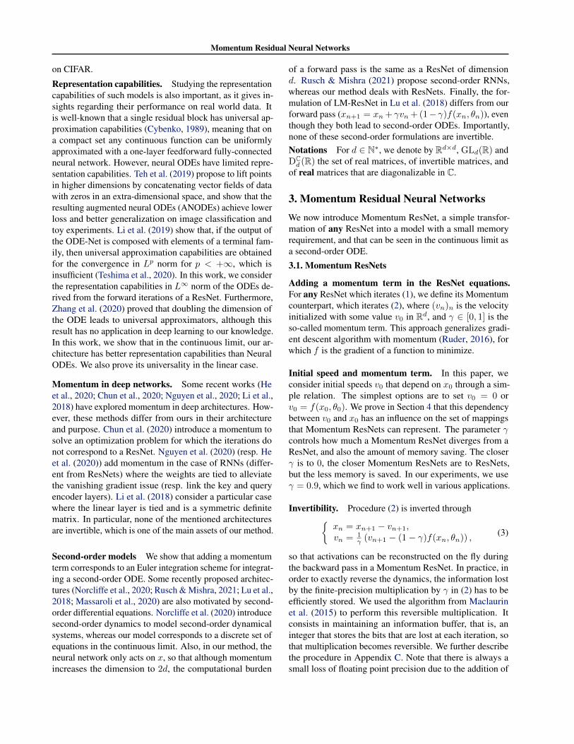
where f is a parameterized function, v is a velocity term andγ ∈ [0, 1] is a momentum term. This radically changes thedynamics of the network, as shown in the following figure.

Input

Momentum ResNet Output

Input

Dep

th

ResNet Output

Figure 1. Comparison of the dynamics of a ResNet (left) anda Momentum ResNet with γ = 0.9 (right) with tied weightsbetween layers, θn = θ for all n. The evolution of the activationsat each layer is shown (depth 15). Models try to learn the mappingx 7→ −x3 in R. The ResNet fails (the iterations approximate thesolution of a first-order ODE, for which trajectories don’t cross, cf.Picard-Lindelof theorem) while the Momentum ResNet leveragesthe changes in velocity to model more complex dynamics.

In contrast with existing reversible models, MomentumResNets can be integrated seamlessly in any deep architec-

arX

iv:2

102.

0787

0v3

[cs

.LG

] 2

2 Ju

l 202

1


ture which uses residual blocks as building blocks (cf. inSection 3).

Contributions. We introduce momentum residual neuralnetworks (Momentum ResNets), a new deep model thatrelies on a simple modification of the ResNet forward ruleand which, without any constraint on its architecture, isperfectly invertible. We show that the memory requirementof Momentum ResNets is arbitrarily reduced by changingthe momentum term γ (Section 3.2), and show that they canbe used as a drop-in replacement for traditional ResNets.

On the theoretical side, we show that Momentum ResNetsare easily used in the learning to optimize setting, whereother reversible models fail to converge (Section 3.3). Wealso investigate the approximation capabilities of Momen-tum ResNets, seen in the continuous limit as second-orderODEs (Section 4). We first show in Proposition 3 thatMomentum ResNets can represent a strictly larger classof functions than first-order neural ODEs. Then, we givemore detailed insights by studying the linear case, wherewe formally prove in Theorem 1 that Momentum ResNetswith linear residual functions have universal approximationcapabilities, and precisely quantify how the set of repre-sentable mappings for such models grows as the momentumterm γ increases. This theoretical result is a first step to-wards a theoretical analysis of representation capabilities ofMomentum ResNets.

Our last contribution is the experimental validation of Mo-mentum ResNets on various learning tasks. We first showthat Momentum ResNets separate point clouds that ResNetsfail to separate (Section 5.1). We also show on imagedatasets (CIFAR-10, CIFAR-100, ImageNet) that Momen-tum ResNets have similar accuracy as ResNets, with asmaller memory cost (Section 5.2). We also show thatparameters of a pre-trained model are easily transferred to aMomentum ResNet which achieves comparable accuracy inonly few epochs of training. We argue that this way to ob-tain pre-trained Momentum ResNets is of major importancefor fine-tuning a network on new data for which memorystorage is a bottleneck. We provide a Pytorch package with amethod that takes a torchvision ResNet model and returns itsMomentum counterpart that achieves similar accuracy withvery little refit. We also experimentally validate our theoret-ical findings in the learning to optimize setting, by confirm-ing that Momentum ResNets perform better than RevNets(Gomez et al., 2017). Our code is available at https://github.com/michaelsdr/momentumnet.

2. Background and previous works.Backpropagation. Backpropagation is the method ofchoice to compute the gradient of a scalar-valued function.It operates using the chain rule with a backward traversal ofthe computational graph (Bauer, 1974). It is also known as

reverse-mode automatic differentiation (Baydin et al., 2018;Rumelhart et al., 1986; Verma, 2000; Griewank & Walther,2008). The computational cost is similar to the one of eval-uating the function itself. The only way to back-propagategradients through a neural architecture without further as-sumptions is to store all the intermediate activations duringthe forward pass. This is the method used in common deeplearning libraries such as Pytorch (Paszke et al., 2017), Ten-sorflow (Abadi et al., 2016) and JAX (Jacobsen et al., 2018).A common way to reduce this memory storage is to usecheckpointing: activations are only stored at some steps andthe others are recomputed between these check-points asthey become needed in the backward pass (e.g., Martens &Sutskever (2012)).

Reversible architectures. However, models that allowbackpropagation without storing any activations have re-cently been developed. They are based on two kinds ofapproaches. The first is discrete and relies on finding waysto easily invert the rule linking activation n to activation n+1(Gomez et al., 2017; Chang et al., 2018; Haber & Ruthotto,2017; Jacobsen et al., 2018; Behrmann et al., 2019). In thisway, it is possible to recompute the activations on the fly dur-ing the backward pass: activations do not have to be stored.However, these methods either rely on restricted architec-tures where there is no straightforward way to transfer a wellperforming non-reversible model into a reversible one, or donot offer a fast inversion scheme when recomputing activa-tions backward. In contrast, our proposal can be applied toany existing ResNet and is easily inverted. The second kindof approach is continuous and relies on ordinary differentialequations (ODEs), where ResNets are interpreted as contin-uous dynamical systems (Weinan, 2017; Chen et al., 2018;Teh et al., 2019; Sun et al., 2018; Weinan et al., 2019; Luet al., 2018; Ruthotto & Haber, 2019). This allows one to im-port theoretical and numerical advances from ODEs to deeplearning. These models are often called neural ODEs (Chenet al., 2018) and can be trained by using an adjoint sensi-tivity method (Pontryagin, 2018), solving ODEs backwardin time. This strategy avoids performing reverse-mode au-tomatic differentiation through the operations of the ODEsolver and leads to a O(1) memory footprint. However,defining the neural ODE counterpart of an existing residualarchitecture is not straightforward: optimizing ODE blocksis an infinite dimensional problem requiring a non-trivialtime discretization, and the performances of neural ODEsdepend on the numerical integrator for the ODE (Gusaket al., 2020). In addition, ODEs cannot always be numeri-cally reversed, because of stability issues: numerical errorscan occur and accumulate when a system is run backwards(Gholami et al., 2019; Teh et al., 2019). Thus, in practice,neural ODEs are seldom used in standard deep learningsettings. Nevertheless, recent works (Zhang et al., 2019;Queiruga et al., 2020) incorporate ODE blocks in neuralarchitectures to achieve comparable accuracies to ResNets

https://github.com/michaelsdr/momentumnet

https://github.com/michaelsdr/momentumnet


on CIFAR.

Representation capabilities. Studying the representationcapabilities of such models is also important, as it gives in-sights regarding their performance on real world data. Itis well-known that a single residual block has universal ap-proximation capabilities (Cybenko, 1989), meaning that ona compact set any continuous function can be uniformlyapproximated with a one-layer feedforward fully-connectedneural network. However, neural ODEs have limited repre-sentation capabilities. Teh et al. (2019) propose to lift pointsin higher dimensions by concatenating vector fields of datawith zeros in an extra-dimensional space, and show that theresulting augmented neural ODEs (ANODEs) achieve lowerloss and better generalization on image classification andtoy experiments. Li et al. (2019) show that, if the output ofthe ODE-Net is composed with elements of a terminal fam-ily, then universal approximation capabilities are obtainedfor the convergence in Lp norm for p < +∞, which isinsufficient (Teshima et al., 2020). In this work, we considerthe representation capabilities in L∞ norm of the ODEs de-rived from the forward iterations of a ResNet. Furthermore,Zhang et al. (2020) proved that doubling the dimension ofthe ODE leads to universal approximators, although thisresult has no application in deep learning to our knowledge.In this work, we show that in the continuous limit, our ar-chitecture has better representation capabilities than NeuralODEs. We also prove its universality in the linear case.

Momentum in deep networks. Some recent works (Heet al., 2020; Chun et al., 2020; Nguyen et al., 2020; Li et al.,2018) have explored momentum in deep architectures. How-ever, these methods differ from ours in their architectureand purpose. Chun et al. (2020) introduce a momentum tosolve an optimization problem for which the iterations donot correspond to a ResNet. Nguyen et al. (2020) (resp. Heet al. (2020)) add momentum in the case of RNNs (differ-ent from ResNets) where the weights are tied to alleviatethe vanishing gradient issue (resp. link the key and queryencoder layers). Li et al. (2018) consider a particular casewhere the linear layer is tied and is a symmetric definitematrix. In particular, none of the mentioned architecturesare invertible, which is one of the main assets of our method.

Second-order models We show that adding a momentumterm corresponds to an Euler integration scheme for integrat-ing a second-order ODE. Some recently proposed architec-tures (Norcliffe et al., 2020; Rusch & Mishra, 2021; Lu et al.,2018; Massaroli et al., 2020) are also motivated by second-order differential equations. Norcliffe et al. (2020) introducesecond-order dynamics to model second-order dynamicalsystems, whereas our model corresponds to a discrete set ofequations in the continuous limit. Also, in our method, theneural network only acts on x, so that although momentumincreases the dimension to 2d, the computational burden

of a forward pass is the same as a ResNet of dimensiond. Rusch & Mishra (2021) propose second-order RNNs,whereas our method deals with ResNets. Finally, the for-mulation of LM-ResNet in Lu et al. (2018) differs from ourforward pass (xn+1 = xn + γvn + (1− γ)f(xn, θn)), eventhough they both lead to second-order ODEs. Importantly,none of these second-order formulations are invertible.Notations For d ∈ N∗, we denote by Rd×d, GLd(R) andDCd (R) the set of real matrices, of invertible matrices, and

of real matrices that are diagonalizable in C.

3. Momentum Residual Neural NetworksWe now introduce Momentum ResNet, a simple transfor-mation of any ResNet into a model with a small memoryrequirement, and that can be seen in the continuous limit asa second-order ODE.

3.1. Momentum ResNets

Adding a momentum term in the ResNet equations.For any ResNet which iterates (1), we define its Momentumcounterpart, which iterates (2), where (vn)n is the velocityinitialized with some value v0 in Rd, and γ ∈ [0, 1] is theso-called momentum term. This approach generalizes gradi-ent descent algorithm with momentum (Ruder, 2016), forwhich f is the gradient of a function to minimize.

Initial speed and momentum term. In this paper, weconsider initial speeds v0 that depend on x0 through a sim-ple relation. The simplest options are to set v0 = 0 orv0 = f(x0, θ0). We prove in Section 4 that this dependencybetween v0 and x0 has an influence on the set of mappingsthat Momentum ResNets can represent. The parameter γcontrols how much a Momentum ResNet diverges from aResNet, and also the amount of memory saving. The closerγ is to 0, the closer Momentum ResNets are to ResNets,but the less memory is saved. In our experiments, we useγ = 0.9, which we find to work well in various applications.

Invertibility. Procedure (2) is inverted through{xn = xn+1 − vn+1,vn = 1

γ (vn+1 − (1− γ)f(xn, θn)) ,(3)

so that activations can be reconstructed on the fly duringthe backward pass in a Momentum ResNet. In practice, inorder to exactly reverse the dynamics, the information lostby the finite-precision multiplication by γ in (2) has to beefficiently stored. We used the algorithm from Maclaurinet al. (2015) to perform this reversible multiplication. Itconsists in maintaining an information buffer, that is, aninteger that stores the bits that are lost at each iteration, sothat multiplication becomes reversible. We further describethe procedure in Appendix C. Note that there is always asmall loss of floating point precision due to the addition of


the learnable mapping f . In practice, we never found it to bea problem: this loss in precision can be neglected comparedto the one due to the multiplication by γ.

Table 1. Comparison of reversible residual architectures

Neu

r.OD

E

i-Res

Net

i-Rev

Net

Rev

Net

Mom

.Net

Closed-form inversion 3 7 3 3 3

Same parameters 7 3 7 7 3

Unconstrained training 3 7 3 3 3

Drop-in replacement. Our approach makes it possibleto turn any existing ResNet into a reversible one. In otherwords, a ResNet can be transformed into its Momentumcounterpart without changing the structure of each layer.For instance, consider a ResNet-152 (He et al., 2016). It ismade of 4 layers (of depth 3, 8, 36 and 3) and can easily beturned into its Momentum ResNet counterpart by changingthe forward equations (1) into (2) in the 4 layers. No furtherchange is needed and Momentum ResNets take the exactsame parameters as inputs: they are a drop-in replacement.This is not the case of other reversible models. Neural ODEs(Chen et al., 2018) take continuous parameters as inputs. i-ResNets (Behrmann et al., 2019) cannot be trained by plainSGD since the spectral norm of the weights requires con-strained optimization. i-RevNets (Jacobsen et al., 2018) andRevNets (Gomez et al., 2017) require to train two networkswith their own parameters for each residual block, split theinputs across convolutional channels, and are half as deepas ResNets: they do not take the same parameters as inputs.Table 1 summarizes the properties of reversible residualarchitectures. We discuss in further details the differencesbetween RevNets and Momentum ResNets in sections 3.3and 5.3.

3.2. Memory cost

Instead of storing the full data at each layer, we only needto store the bits lost at each multiplication by γ (cf. “intert-ibility”). For an architecture of depth k, this correspondsto storing log2(( 1

γ )k) values for each sample (k(1−γ)ln(2) ifγ is close to 1). To illustrate, we consider two situationswhere storing the activations is by far the main memorybottleneck. First, consider a toy feedforward architecturewhere f(x, θ) = WT

2 σ(W1x + b), with x ∈ Rd andθ = (W1,W2, b), where W1,W2 ∈ Rp×d and b ∈ Rp,with a depth k ∈ N. We suppose that the weights are thesame at each layer. The training set is composed of n vec-tors x1, ..., xn ∈ Rd. For ResNets, we need to store theweights of the network and the values of all activations forthe training set at each layer of the network. In total, the

memory needed is O(k × d× nbatch) per iteration. In thecase of Momentum ResNets, if γ is close to 1 we get amemory requirement of O((1− γ)× k× d× nbatch). Thisproves that the memory dependency in the depth k is arbi-trarily reduced by changing the momentum γ. The memorysavings are confirmed in practice, as shown in Figure 2.

0 200 400 600 800

Depth

102

103

Mem

ory

(MiB

)

ResNet

Momentum ResNet

Figure 2. Comparison of memory needed (calculated using aprofiler) for computing gradients of the loss, with ResNets (acti-vations are stored) and Momentum ResNets (activations are notstored). We set nbatch = 500, d = 500 and γ = 1 − 1

50kat

each depth. Momentum ResNets give a nearly constant memoryfootprint.

As another example, consider a ResNet-152 (He et al., 2016)which can be used for ImageNet classification (Deng et al.,2009). Its layer named “conv4 x” has a depth of 36: ithas 40 M parameters, whereas storing the activations wouldrequire storing 50 times more parameters. Since storingthe activations is here the main obstruction, the memoryrequirement for this layer can be arbitrarily reduced bytaking γ close to 1.

3.3. The role of momentum

When γ is set to 0 in (2), we recover a ResNet. Therefore,Momentum ResNets are a generalization of ResNets. Whenγ −→ 1, one can scale f → 1

1−γ f to get in (2) a symplecticscheme (Hairer et al., 2006) that recovers a special case ofother popular invertible neural network: RevNets (Gomezet al., 2017) and Hamiltonian Networks (Chang et al., 2018).A RevNet iterates

vn+1 = vn+ϕ(xn, θn), xn+1 = xn+ψ(vn+1, θ′

n), (4)

where ϕ and ψ are two learnable functions.

The usefulness of such architecture depends on the task.RevNets have encountered success for classification andregression. However, we argue that RevNets cannot workin some settings. For instance, under mild assumptions,the RevNet iterations do not have attractive fixed pointswhen the parameters are the same at each layer: θn = θ,θ′n = θ′. We rewrite (4) as (vn+1, xn+1) = Ψ(vn, xn) withΨ(v, x) = (v + ϕ(x, θ), x+ ψ(v + ϕ(x, θ), θ′)).

Proposition 1 (Instability of fixed points). Let (v∗, x∗) afixed point of the RevNet iteration (4). Assume that ϕ (resp.ψ) is differentiable at x∗ (resp. v∗), with Jacobian matrixA (resp. B) ∈ Rd×d. The Jacobian of Ψ at (v∗, x∗) is


J(A,B) =(Idd AB Idd+BA

). If A and B are invertible, then

there exists λ ∈ Sp (J(A,B)) such that |λ| ≥ 1 and λ 6= 1.

This shows that (v∗, x∗) cannot be a stable fixed point. As aconsequence, in practice, a RevNet cannot have convergingiterations: according to (4), if xn converges then vn mustalso converge, and their limit must be a fixed point. Theprevious proposition shows that it is impossible.

This result suggests that RevNets should perform poorly inproblems where one expects the iterations of the networkto converge. For instance, as shown in the experiments inSection 5.3, this happens when we use reverible dynamicsin order to learn to optimize (Maclaurin et al., 2015). Incontrast, the proposed method can converge to a fixed pointas long as the momentum term γ is strictly less than 1.Remark. Proposition 1 has a continuous counterpart. In-deed, in the continuous limit, (4) writes v = ϕ(x, θ), x =ψ(v, θ′). The corresponding Jacobian in (v∗, x∗) is

(0 AB 0

).

The eigenvalues of this matrix are the square roots of thoseof AB: they cannot all have a real part < 0 (same stabilityissue in the continuous case).

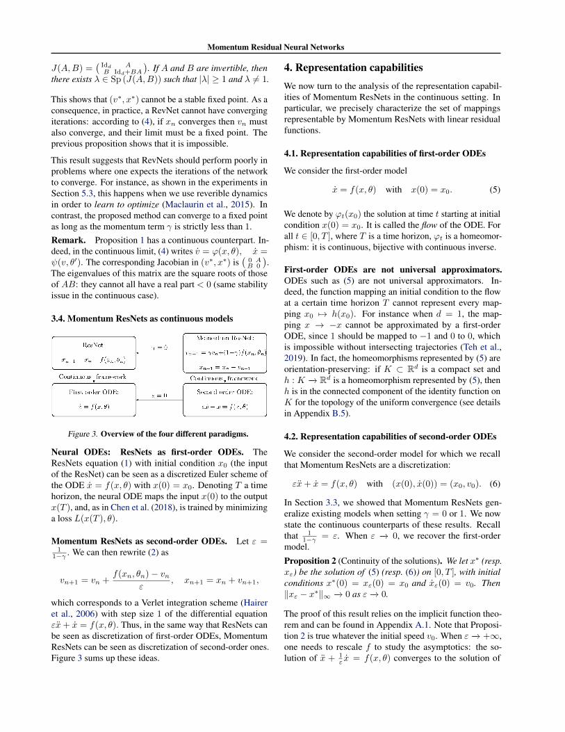
3.4. Momentum ResNets as continuous models

Figure 3. Overview of the four different paradigms.

Neural ODEs: ResNets as first-order ODEs. TheResNets equation (1) with initial condition x0 (the inputof the ResNet) can be seen as a discretized Euler scheme ofthe ODE x = f(x, θ) with x(0) = x0. Denoting T a timehorizon, the neural ODE maps the input x(0) to the outputx(T ), and, as in Chen et al. (2018), is trained by minimizinga loss L(x(T ), θ).

Momentum ResNets as second-order ODEs. Let ε =1

1−γ . We can then rewrite (2) as

vn+1 = vn +f(xn, θn)− vn

ε, xn+1 = xn + vn+1,

which corresponds to a Verlet integration scheme (Haireret al., 2006) with step size 1 of the differential equationεx+ x = f(x, θ). Thus, in the same way that ResNets canbe seen as discretization of first-order ODEs, MomentumResNets can be seen as discretization of second-order ones.Figure 3 sums up these ideas.

4. Representation capabilitiesWe now turn to the analysis of the representation capabil-ities of Momentum ResNets in the continuous setting. Inparticular, we precisely characterize the set of mappingsrepresentable by Momentum ResNets with linear residualfunctions.

4.1. Representation capabilities of first-order ODEs

We consider the first-order model

x = f(x, θ) with x(0) = x0. (5)

We denote by ϕt(x0) the solution at time t starting at initialcondition x(0) = x0. It is called the flow of the ODE. Forall t ∈ [0, T ], where T is a time horizon, ϕt is a homeomor-phism: it is continuous, bijective with continuous inverse.

First-order ODEs are not universal approximators.ODEs such as (5) are not universal approximators. In-deed, the function mapping an initial condition to the flowat a certain time horizon T cannot represent every map-ping x0 7→ h(x0). For instance when d = 1, the map-ping x → −x cannot be approximated by a first-orderODE, since 1 should be mapped to −1 and 0 to 0, whichis impossible without intersecting trajectories (Teh et al.,2019). In fact, the homeomorphisms represented by (5) areorientation-preserving: if K ⊂ Rd is a compact set andh : K −→ Rd is a homeomorphism represented by (5), thenh is in the connected component of the identity function onK for the topology of the uniform convergence (see detailsin Appendix B.5).

4.2. Representation capabilities of second-order ODEs

We consider the second-order model for which we recallthat Momentum ResNets are a discretization:

εx+ x = f(x, θ) with (x(0), x(0)) = (x0, v0). (6)

In Section 3.3, we showed that Momentum ResNets gen-eralize existing models when setting γ = 0 or 1. We nowstate the continuous counterparts of these results. Recallthat 1

1−γ = ε. When ε −→ 0, we recover the first-ordermodel.

Proposition 2 (Continuity of the solutions). We let x∗ (resp.xε) be the solution of (5) (resp. (6)) on [0, T ], with initialconditions x∗(0) = xε(0) = x0 and xε(0) = v0. Then‖xε − x∗‖∞ −→ 0 as ε −→ 0.

The proof of this result relies on the implicit function theo-rem and can be found in Appendix A.1. Note that Proposi-tion 2 is true whatever the initial speed v0. When ε −→ +∞,one needs to rescale f to study the asymptotics: the so-lution of x + 1

ε x = f(x, θ) converges to the solution of


x = f(x, θ) (see details in Appendix B.1). These resultsshow that in the continuous regime, Momentum ResNetsalso interpolate between x = f(x, θ) and x = f(x, θ).

Representation capabilities of a model (6) on the xspace. We recall that we consider initial speeds v0 thatcan depend on the input x0 ∈ Rd (for instance v0 = 0or v0 = f(x0, θ0)). We therefore assume ϕt : Rd 7→Rd such that ϕt(x0) is solution of (6). We emphasizethat ϕt is not always a homeomorphism. For instance,ϕt(x0) = x0 exp (−t/2) cos (t/2) solves x+ x = − 1

2x(t)with (x(0), x(0)) = (x0,−x0

2 ). All the trajectories inter-sect at time π. It means that Momentum ResNets can learnmappings that are not homeomorphisms, which suggeststhat increasing ε should lead to better representation capa-bilities. The first natural question is thus whether, givenh : Rd −→ Rd, there exists some f such that ϕt asso-ciated to (6) satisfies ∀x ∈ Rd, ϕ1(x) = h(x). In thecase where v0 is an arbitrary function of x0, the answeris trivial since (6) can represent any mapping, as provedin Appendix B.2. This setting does not correspond to thecommon use case of ResNets, which take advantage of theirdepth, so it is important to impose stronger constraints onthe dependency between v0 and x0. For instance, the nextproposition shows that even if one imposes v0 = f(x0, θ0),a second-order model is at least as general as a first-orderone.

Proposition 3 (Momentum ResNets are at least as general).There exists a function f such that for all x solution of (5), xis also solution of the second-order model εx+ x = f(x, θ)with (x(0), x(0)) = (x0, f(x0, θ0)).

Furthermore, even with the restrictive initial condition v0 =0, x 7→ λx for λ > −1 can always be represented by asecond-order model (6) (see details in Appendix B.4). Thissupports the claim that the set of representable mappingsincreases with ε.

4.3. Universality of Momentum ResNets with linearresidual functions

As a first step towards a theoretical analysis of the universalrepresentation capabilities of Momentum ResNets, we nowinvestigate the linear residual function case. Consider thesecond-order linear ODE

εx+ x = θx with (x(0), x(0)) = (x0, 0), (7)

with θ ∈ Rd×d. We assume without loss of generality thatthe time horizon is T = 1. We have the following result.

Proposition 4 (Solution of (7)). At time 1, (7) defines thelinear mapping x0 7→ ϕ1(x0) = Ψε(θ)x0 where

Ψε(θ) = e−12ε

+∞∑n=0

(1

(2n)!+

1

2ε(2n+ 1)!

)(θ

ε+

Idd4ε2

)n.

Characterizing the set of mappings representable by (7) isthus equivalent to precisely analyzing the range Ψε(Rd×d).

Representable mappings of a first-order linear model.When ε −→ 0, Proposition 2 shows that Ψε(θ) −→ Ψ0(θ) =exp θ. The range of the matrix exponential is indeed the setof representable mappings of a first order linear model

x = θx with x(0) = x0 (8)

and this range is known (Andrica & Rohan, 2010) to beΨ0(Rd×d) = exp (Rd×d) = {M2 | M ∈ GLd(R)}. Thismeans that one can only learn mappings that are the squareof invertible mappings with a first-order linear model (8).To ease the exposition and exemplify the impact of increas-ing ε > 0, we now consider the case of matrices with realcoefficients that are diagonalizable in C, DC

d (R). Note thatthe general setting of arbitrary matrices is exposed in Ap-pendix A.4 using Jordan decomposition. Note also thatDCd (R) is dense in Rd×d (Hartfiel, 1995). Using Theorem 1

from Culver (1966), we have that if D ∈ DCd (R), then D

is represented by a first-order model (8) if and only if Dis non-singular and for all eigenvalues λ ∈ Sp(D) withλ < 0, λ is of even multiplicity order. This is restrictivebecause it forces negative eigenvalues to be in pairs. Wenow generalize this result and show that increasing ε > 0leads to less restrictive conditions.

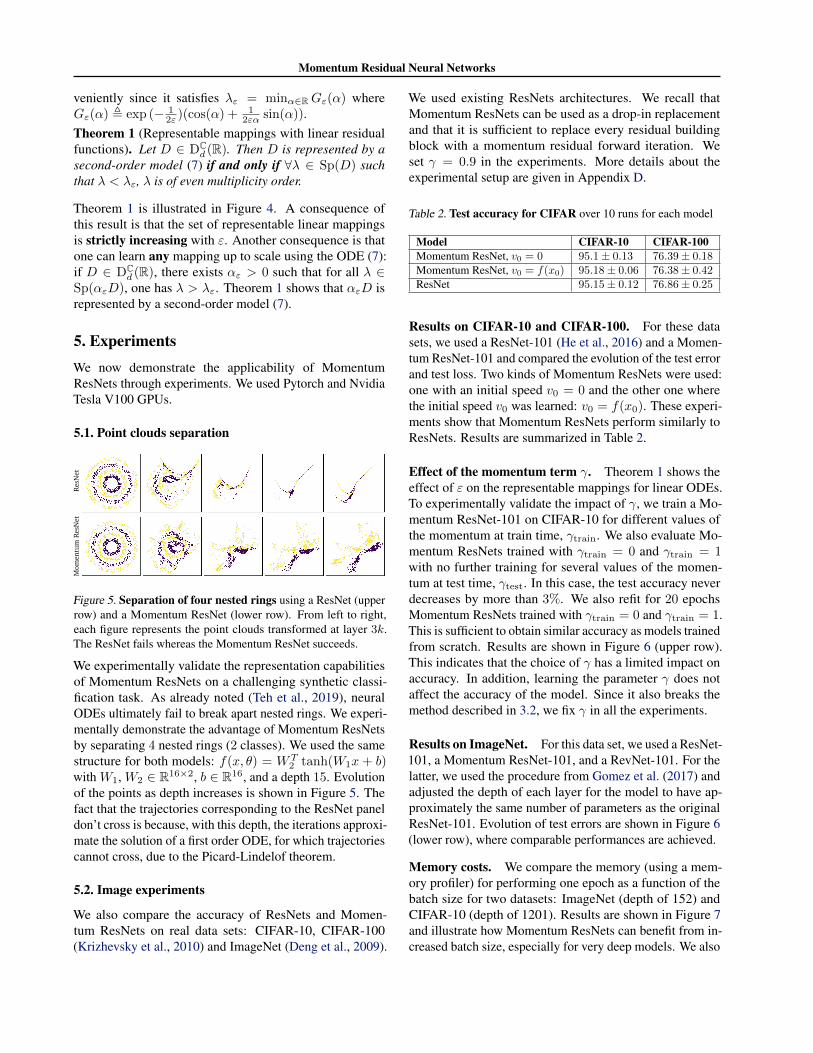
ε = + ∞ε = 0.5

ε = 0

−1−

−1|

λ1

λ2

ε

λε

Figure 4. Left: Evolution of λε defined in Theorem 1. λε is nonincreasing, stays close to 0 when ε � 1 and close to −1 whenε ≥ 2. Right: Evolution of the real eigenvalues λ1 and λ2 ofrepresentable matrices in DC

d(R) by (7) when d = 2 for differentvalues of ε. The grey colored areas correspond to the differentrepresentable eigenvalues. When ε = 0, λ1 = λ2 or λ1 > 0 andλ2 > 0. When ε > 0, single negative eigenvalues are acceptable.

Representable mappings by a second-order linearmodel. Again, by density and for simplicity, we focuson matrices in DC

d (R), and we state and prove the gen-eral case in Appendix A.4, making use of Jordan blocksdecomposition of matrix functions (Gantmacher, 1959)and localization of zeros of entire functions (Runckel,1969). The range of Ψε over the reals has for formΨε(R) = [λε,+∞[. It plays a pivotal role to controlthe set of representable mappings, as stated in the theo-rem bellow. Its minimum value can be computed con-


veniently since it satisfies λε = minα∈RGε(α) whereGε(α) , exp (− 1

2ε )(cos(α) + 12εα sin(α)).

Theorem 1 (Representable mappings with linear residualfunctions). Let D ∈ DC

d (R). Then D is represented by asecond-order model (7) if and only if ∀λ ∈ Sp(D) suchthat λ < λε, λ is of even multiplicity order.

Theorem 1 is illustrated in Figure 4. A consequence ofthis result is that the set of representable linear mappingsis strictly increasing with ε. Another consequence is thatone can learn any mapping up to scale using the ODE (7):if D ∈ DC

d (R), there exists αε > 0 such that for all λ ∈Sp(αεD), one has λ > λε. Theorem 1 shows that αεD isrepresented by a second-order model (7).

5. ExperimentsWe now demonstrate the applicability of MomentumResNets through experiments. We used Pytorch and NvidiaTesla V100 GPUs.

5.1. Point clouds separation

Mom

entu

m R

esN

etRe

sNet

Figure 5. Separation of four nested rings using a ResNet (upperrow) and a Momentum ResNet (lower row). From left to right,each figure represents the point clouds transformed at layer 3k.The ResNet fails whereas the Momentum ResNet succeeds.

We experimentally validate the representation capabilitiesof Momentum ResNets on a challenging synthetic classi-fication task. As already noted (Teh et al., 2019), neuralODEs ultimately fail to break apart nested rings. We experi-mentally demonstrate the advantage of Momentum ResNetsby separating 4 nested rings (2 classes). We used the samestructure for both models: f(x, θ) = WT

2 tanh(W1x + b)with W1, W2 ∈ R16×2, b ∈ R16, and a depth 15. Evolutionof the points as depth increases is shown in Figure 5. Thefact that the trajectories corresponding to the ResNet paneldon’t cross is because, with this depth, the iterations approxi-mate the solution of a first order ODE, for which trajectoriescannot cross, due to the Picard-Lindelof theorem.

5.2. Image experiments

We also compare the accuracy of ResNets and Momen-tum ResNets on real data sets: CIFAR-10, CIFAR-100(Krizhevsky et al., 2010) and ImageNet (Deng et al., 2009).

We used existing ResNets architectures. We recall thatMomentum ResNets can be used as a drop-in replacementand that it is sufficient to replace every residual buildingblock with a momentum residual forward iteration. Weset γ = 0.9 in the experiments. More details about theexperimental setup are given in Appendix D.

Table 2. Test accuracy for CIFAR over 10 runs for each model

Model CIFAR-10 CIFAR-100Momentum ResNet, v0 = 0 95.1± 0.13 76.39± 0.18Momentum ResNet, v0 = f(x0) 95.18± 0.06 76.38± 0.42ResNet 95.15± 0.12 76.86± 0.25

Results on CIFAR-10 and CIFAR-100. For these datasets, we used a ResNet-101 (He et al., 2016) and a Momen-tum ResNet-101 and compared the evolution of the test errorand test loss. Two kinds of Momentum ResNets were used:one with an initial speed v0 = 0 and the other one wherethe initial speed v0 was learned: v0 = f(x0). These experi-ments show that Momentum ResNets perform similarly toResNets. Results are summarized in Table 2.

Effect of the momentum term γ. Theorem 1 shows theeffect of ε on the representable mappings for linear ODEs.To experimentally validate the impact of γ, we train a Mo-mentum ResNet-101 on CIFAR-10 for different values ofthe momentum at train time, γtrain. We also evaluate Mo-mentum ResNets trained with γtrain = 0 and γtrain = 1with no further training for several values of the momen-tum at test time, γtest. In this case, the test accuracy neverdecreases by more than 3%. We also refit for 20 epochsMomentum ResNets trained with γtrain = 0 and γtrain = 1.This is sufficient to obtain similar accuracy as models trainedfrom scratch. Results are shown in Figure 6 (upper row).This indicates that the choice of γ has a limited impact onaccuracy. In addition, learning the parameter γ does notaffect the accuracy of the model. Since it also breaks themethod described in 3.2, we fix γ in all the experiments.

Results on ImageNet. For this data set, we used a ResNet-101, a Momentum ResNet-101, and a RevNet-101. For thelatter, we used the procedure from Gomez et al. (2017) andadjusted the depth of each layer for the model to have ap-proximately the same number of parameters as the originalResNet-101. Evolution of test errors are shown in Figure 6(lower row), where comparable performances are achieved.

Memory costs. We compare the memory (using a mem-ory profiler) for performing one epoch as a function of thebatch size for two datasets: ImageNet (depth of 152) andCIFAR-10 (depth of 1201). Results are shown in Figure 7and illustrate how Momentum ResNets can benefit from in-creased batch size, especially for very deep models. We also


0.0 0.2 0.4 0.6 0.8 1.0

Momentum at test time γtest

93

94

95

Tes

tA

ccu

racy

γtrain = γtest, full training

γtrain = 1, no refit

γtrain = 1, refit for 20 epochs

0.0 0.2 0.4 0.6 0.8 1.0

Momentum at test time γtest

93

94

95

Tes

tA

ccu

racy

γtrain = γtest, full training

γtrain = 0, no refit

γtrain = 0, refit for 20 epochs

0 25 50 75 100

Iterations

20%

30%

40%

50%

Tes

ter

ror

ResNet

Momentum ResNet (v0 = 0)

Momentum ResNet (v0 = f(x0))

RevNet

Figure 6. Upper row: Robustness of final accuracy w.r.t γ when training Momentum ResNets 101 on CIFAR-10. We train the networkswith a momentum γtrain and evaluate their accuracy with a different momentum γtest at test time. We optionally refit the networksfor 20 epochs. We recall that γtrain = 0 corresponds to a classical ResNet and γtrain = 1 corresponds to a Momentum ResNet withoptimal memory savings. Lower row: Top-1 classification error on ImageNet (single crop) for 4 different residual architectures ofdepth 101 with the same number of parameters. Final test accuracy is 22% for the ResNet-101 and 23% for the 3 other invertible models.In particular, our model achieve the same performance as a RevNet with the same number of parameters.

show in Figure 7 the final test accuracy for a full trainingof Momentum ResNets on CIFAR-10 as a function of thememory used (directly linked to γ (section 3.2)).

32 64 128 256

Batch Size

8

16

32

Mem

ory

(Gib

)

Out of memoryOut of memory

ImageNet, depth 152

ResNet

Momentum ResNet

32 128 512 2048

Batch Size

8

16

32Out of memoryOut of memory

CIFAR-10, depth 1201

5 6 7 8 9 10

Memory (GiB)

95.0

95.2

95.4

Tes

tA

ccur

acy

Final test accuracy as function of the memory

Full training

Memory (GiB)

95

95

Tes

tAcc

urac

y

5 6 7 8 9 10

Memory (GiB)

95.0

95.2

95.4

Tes

tA

ccur

acy


Full training

5 6 7 8 9 10

Memory (GiB)

95.0

95.2

95.4

Tes

tAcc

urac

y


Momentum ResNet

RevNet

Figure 7. Upper row: Memory used (using a profiler) for a ResNetand a Momentum ResNet on one training epoch, as a function ofthe batch size. Lower row: Final test accuracy as a function ofthe memory used (per epoch) for training Momentum ResNets-101on CIFAR-10.

Ability to perform pre-training and fine-tuning. It hasbeen shown (Tajbakhsh et al., 2016) that in various medi-cal imaging applications the use of a pre-trained model onImageNet with adapted fine-tuning outperformed a modeltrained from scratch. In order to easily obtain pre-trainedMomentum ResNets for applications where memory couldbe a bottleneck, we transferred the learned parameters ofa ResNet-152 pre-trained on ImageNet to a MomentumResNet-152 with γ = 0.9. In only 1 epoch of additionaltraining we reached a top-1 error of 26.5% and in 5 addi-tional epochs a top-1 error of 23.5%. We then empirically

compared the accuracy of these pre-trained models by fine-tuning them on new images: the hymenoptera1 data set.

0 10 20

Training time (sec.)

60%

80%

90%

Tes

tac

cura

cy

ResNet

Momentum ResNet

Figure 8. Accuracy asa function of time onhymenoptera when fine-tuning a ResNet-152 anda Momentum ResNet-152with batch sizes of 2 and 4,respectively, as permittedby memory.

As a proof of concept, suppose we have a GPU with 3 Goof RAM. The images have a resolution of 500× 500 pixelsso that the maximum batch size that can be taken for fine-tuning the ResNet-152 is 2, against 4 for the MomentumResNet-152. As suggested in Tajbakhsh et al. (2016) (“ifthe distance between the source and target applications issignificant, one may need to fine-tune the early layers aswell”), we fine-tune the whole network in this proof ofconcept experiment. In this setting the Momentum ResNetleads to faster convergence when fine-tuning, as shownin Figure 8: Momentum ResNets can be twice as fast asResNets to train when samples are so big that only fewof them can be processed at a time. In contrast, RevNets(Gomez et al., 2017) cannot as easily be used for fine-tuningsince, as shown in (4), they require to train two distinctnetworks.

Continuous training. We also compare accuracy whenusing first-order ODE blocks (Chen et al., 2018) and second-order ones on CIFAR-10. In order to emphasize the in-fluence of the ODE, we considered a neural architecturewhich down-sampled the input to have a certain number ofchannels, and then applied 10 successive ODE blocks. Twotypes of blocks were considered: one corresponded to thefirst-order ODE (5) and the other one to the second-orderODE (6). Training was based on the odeint function imple-

1https://www.kaggle.com/ajayrana/hymenoptera-data


mented by Chen et al. (2018). Figure 9 shows the final testaccuracy for both models as a function of the number ofchannels used. As a baseline, we also include the final accu-racy when there are no ODE blocks. We see that an ODENet with momentum significantly outperforms an originalODE Net when the number of channels is small. Trainingtook the same time for both models.

4 8 16 32

Number of channels

40%

60%

80%

Tes

tac

cura

cy

NODE

NODE Momentum

no ODEFigure 9. Accuracyafter 120 iterationson CIFAR-10 with orwithout momentum,when varying thenumber of channels.

5.3. Learning to optimize

We conclude by illustrating the usefulness of our Momen-tum ResNets in the learning to optimize setting, whereone tries to learn to minimize a function. We considerthe Learned-ISTA (LISTA) framework (Gregor & LeCun,2010). Given a matrix D ∈ Rd×p, and a hyper-parameterλ > 0, the goal is to perform the sparse coding of a vec-tor y ∈ Rd, by finding x ∈ Rp that minimizes the Lassocost function Ly(x) , 1

2‖y −Dx‖2 + λ‖x‖1 (Tibshirani,

1996). In other words, we want to compute a mappingy 7→ argminx Ly(x). The ISTA algorithm (Daubechieset al., 2004) solves the problem, starting from x0 = 0, by it-erating xn+1 = ST(xn− ηD>(Dxn− y), ηλ), with η > 0a step-size. Here, ST is the soft-thresholding operator. Theidea of Gregor & LeCun (2010) is to view L iterations ofISTA as the output of a neural network with L layers that it-erates xn+1 = g(xn, y, θn) , ST(W 1

nxn+W 2ny, ηλ), with

parameters θ , (θ1, . . . , θL) and θn , (W 1n ,W

2n). We call

Φ(y, θ) the network function, which maps y to the output xL.Importantly, this network can be seen as a residual network,with residual function f(x, y, θ) = g(x, y, θ) − x. ISTAcorresponds to fixed parameters between layers: W 1

n =Idp− ηD>D and W 2

n = ηD>, but these parameters can belearned to yield better performance. We focus on an “un-supervised” learning setting, where we have some trainingexamples y1, . . . , yQ, and use them to learn parameters θthat quickly minimize the Lasso function L. In other words,the parameters θ are estimated by minimizing the cost func-tion θ 7→

∑Qq=1 Lyq (Φ(yq, θ)). The performance of the

network is then measured by computing the testing loss,that is the Lasso loss on some unseen testing examples.

We consider a Momentum ResNet and a RevNet variant ofLISTA which use the residual function f . For the RevNet,the activations xn are first duplicated: the network has twiceas many parameters at each layer. The matrixD is generatedwith i.i.d. Gaussian entries with p = 32, d = 16, and its

columns are then normalized to unit variance. Training andtesting samples y are generated as normalized Gaussian i.i.d.entries. More details on the experimental setup are added inAppendix D. The next Figure 10 shows the test loss of thedifferent methods, when the depth of the networks varies.

2 4 6 8Layers

10−1

L−L∗

LISTA Momentum ResNet RevNet ISTA

Figure 10. Evolution of the test loss for different models as afunction of depth in the Learned-ISTA (LISTA) framework.

As predicted by Proposition 1, the RevNet architecture failson this task: it cannot have converging iterations, which isexactly what is expected here. In contrast, the MomentumResNet works well, and even outperforms the LISTA base-line. This is not surprising: it is known that momentum canaccelerate convergence of first order optimization methods.

ConclusionThis paper introduces Momentum ResNets, new invertibleresidual neural networks operating with a significantly re-duced memory footprint compared to ResNets. In sharpcontrast with existing invertible architectures, they are madepossible by a simple modification of the ResNet forwardrule. This simplicity offers both theoretical advantages (bet-ter representation capabilities, tractable analysis of linear dy-namics) and practical ones (drop-in replacement, speed andmemory improvements for model fine-tuning). MomentumResNets interpolate between ResNets (γ = 0) and RevNets(γ = 1), and are a natural second-order extension of neuralODEs. As such, they can capture non-homeomorphic dy-namics and converging iterations. As shown in this paper,the latter is not possible with existing invertible residual net-works, although crucial in the learning to optimize setting.

AcknowledgmentsThis work was granted access to the HPC resources ofIDRIS under the allocation 2020-[AD011012073] madeby GENCI. This work was supported in part by the Frenchgovernment under management of Agence Nationale de laRecherche as part of the “Investissements d’avenir” pro-gram, reference ANR19-P3IA-0001 (PRAIRIE 3IA Insti-tute). This work was supported in part by the European Re-search Council (ERC project NORIA). The authors wouldlike to thank David Duvenaud and Dougal Maclaurin fortheir helpful feedbacks. M. S. thanks Pierre Rizkallah andPierre Roussillon for fruitful discussions.


ReferencesAbadi, M., Agarwal, A., Barham, P., Brevdo, E., Chen, Z.,

Citro, C., Corrado, G. S., Davis, A., Dean, J., Devin,M., et al. Tensorflow: Large-scale machine learningon heterogeneous distributed systems. arXiv preprintarXiv:1603.04467, 2016.

Andrica, D. and Rohan, R.-A. The image of the exponentialmap and some applications. In Proc. 8th Joint Conferenceon Mathematics and Computer Science MaCS, Komarno,Slovakia, pp. 3–14, 2010.

Bauer, F. L. Computational graphs and rounding error. SIAMJournal on Numerical Analysis, 11(1):87–96, 1974.

Baydin, A. G., Pearlmutter, B. A., Radul, A. A., and Siskind,J. M. Automatic differentiation in machine learning: asurvey. Journal of machine learning research, 18, 2018.

Behrmann, J., Grathwohl, W., Chen, R. T., Duvenaud, D.,and Jacobsen, J.-H. Invertible residual networks. InInternational Conference on Machine Learning, pp. 573–582. PMLR, 2019.

Chang, B., Meng, L., Haber, E., Ruthotto, L., Begert, D.,and Holtham, E. Reversible architectures for arbitrarilydeep residual neural networks. In Proceedings of theAAAI Conference on Artificial Intelligence, volume 32,2018.

Chen, T. Q., Rubanova, Y., Bettencourt, J., and Duvenaud,D. K. Neural ordinary differential equations. In Advancesin neural information processing systems, pp. 6571–6583,2018.

Chun, I. Y., Huang, Z., Lim, H., and Fessler, J. Momentum-net: Fast and convergent iterative neural network forinverse problems. IEEE Transactions on Pattern Analysisand Machine Intelligence, 2020.

Conway, J. B. Functions of one complex variable II, volume159. Springer Science & Business Media, 2012.

Craven, T. and Csordas, G. Iterated laguerre and turaninequalities. J. Inequal. Pure Appl. Math, 3(3):14, 2002.

Culver, W. J. On the existence and uniqueness of the reallogarithm of a matrix. Proceedings of the American Math-ematical Society, 17(5):1146–1151, 1966.

Cybenko, G. Approximation by superpositions of a sig-moidal function. Mathematics of control, signals andsystems, 2(4):303–314, 1989.

Daubechies, I., Defrise, M., and De Mol, C. An iterativethresholding algorithm for linear inverse problems with asparsity constraint. Communications on Pure and AppliedMathematics: A Journal Issued by the Courant Instituteof Mathematical Sciences, 57(11):1413–1457, 2004.

Deng, J., Dong, W., Socher, R., Li, L.-J., Li, K., and Fei-Fei,L. Imagenet: A large-scale hierarchical image database.In 2009 IEEE conference on computer vision and patternrecognition, pp. 248–255. Ieee, 2009.

Dryanov, D. and Rahman, Q. Approximation by entirefunctions belonging to the laguerre–polya class. Methodsand Applications of Analysis, 6(1):21–38, 1999.

Gantmacher, F. R. The theory of matrices. Chelsea, NewYork, Vol. I, 1959.

Gholami, A., Keutzer, K., and Biros, G. Anode: Uncondi-tionally accurate memory-efficient gradients for neuralodes. arXiv preprint arXiv:1902.10298, 2019.

Gomez, A. N., Ren, M., Urtasun, R., and Grosse, R. B.The reversible residual network: Backpropagation with-out storing activations. In Guyon, I., Luxburg, U. V.,Bengio, S., Wallach, H., Fergus, R., Vishwanathan, S.,and Garnett, R. (eds.), Advances in Neural InformationProcessing Systems. Curran Associates, Inc., 2017.

Goodfellow, I., Bengio, Y., Courville, A., and Bengio, Y.Deep learning, volume 1. MIT press Cambridge, 2016.

Gregor, K. and LeCun, Y. Learning fast approximations ofsparse coding. In Proceedings of the 27th internationalconferenceon machine learning, pp. 399–406, 2010.

Griewank, A. and Walther, A. Evaluating derivatives:principles and techniques of algorithmic differentiation.SIAM, 2008.

Gusak, J., Markeeva, L., Daulbaev, T., Katrutsa, A., Ci-chocki, A., and Oseledets, I. Towards understand-ing normalization in neural odes. arXiv preprintarXiv:2004.09222, 2020.

Haber, E. and Ruthotto, L. Stable architectures for deepneural networks. Inverse Problems, 34(1):014004, 2017.

Hairer, E., Lubich, C., and Wanner, G. Geometric numericalintegration: structure-preserving algorithms for ordinarydifferential equations, volume 31. Springer Science &Business Media, 2006.

Hartfiel, D. J. Dense sets of diagonalizable matrices. Pro-ceedings of the American Mathematical Society, 123(6):1669–1672, 1995.

He, K., Zhang, X., Ren, S., and Sun, J. Deep residual learn-ing for image recognition. In Proceedings of the IEEEconference on computer vision and pattern recognition,pp. 770–778, 2016.

He, K., Fan, H., Wu, Y., Xie, S., and Girshick, R. Mo-mentum contrast for unsupervised visual representationlearning. In Proceedings of the IEEE/CVF Conference


on Computer Vision and Pattern Recognition, pp. 9729–9738, 2020.

Jacobsen, J.-H., Smeulders, A. W., and Oyallon, E. i-revnet:Deep invertible networks. In International Conferenceon Learning Representations, 2018.

Kolesnikov, A., Beyer, L., Zhai, X., Puigcerver, J., Yung,J., Gelly, S., and Houlsby, N. Big transfer (bit):General visual representation learning. arXiv preprintarXiv:1912.11370, 6(2):8, 2019.

Krizhevsky, A., Nair, V., and Hinton, G. Cifar-10 (canadianinstitute for advanced research). URL http://www. cs.toronto. edu/kriz/cifar. html, 5, 2010.

LeCun, Y., Bengio, Y., and Hinton, G. Deep learning. nature,521(7553):436–444, 2015.

Levin, B. Y. Lectures on entire functions, volume 150.American Mathematical Soc., 1996.

Li, H., Yang, Y., Chen, D., and Lin, Z. Optimization al-gorithm inspired deep neural network structure design.In Asian Conference on Machine Learning, pp. 614–629.PMLR, 2018.

Li, Q., Lin, T., and Shen, Z. Deep learning via dynamicalsystems: An approximation perspective. arXiv preprintarXiv:1912.10382, 2019.

Lu, Y., Zhong, A., Li, Q., and Dong, B. Beyond finite layerneural networks: Bridging deep architectures and numer-ical differential equations. In International Conferenceon Machine Learning, pp. 3276–3285. PMLR, 2018.

Maclaurin, D., Duvenaud, D., and Adams, R. Gradient-based hyperparameter optimization through reversiblelearning. In International conference on machine learn-ing, pp. 2113–2122. PMLR, 2015.

Martens, J. and Sutskever, I. Training deep and recurrentnetworks with hessian-free optimization. In Neural net-works: Tricks of the trade, pp. 479–535. Springer, 2012.

Massaroli, S., Poli, M., Park, J., Yamashita, A., and Asama,H. Dissecting neural odes. In Larochelle, H., Ranzato, M.,Hadsell, R., Balcan, M. F., and Lin, H. (eds.), Advancesin Neural Information Processing Systems, volume 33,pp. 3952–3963. Curran Associates, Inc., 2020.

Nguyen, T. M., Baraniuk, R. G., Bertozzi, A. L., Osher,S. J., and Wang, B. Momentumrnn: Integrating mo-mentum into recurrent neural networks. arXiv preprintarXiv:2006.06919, 2020.

Norcliffe, A., Bodnar, C., Day, B., Simidjievski, N., andLio, P. On second order behaviour in augmented neuralodes. arXiv preprint arXiv:2006.07220, 2020.

Paszke, A., Gross, S., Chintala, S., Chanan, G., Yang, E.,DeVito, Z., Lin, Z., Desmaison, A., Antiga, L., and Lerer,A. Automatic differentiation in pytorch. 2017.

Peng, C., Zhang, X., Yu, G., Luo, G., and Sun, J. Largekernel matters–improve semantic segmentation by globalconvolutional network. In Proceedings of the IEEE con-ference on computer vision and pattern recognition, pp.4353–4361, 2017.

Perko, L. Differential equations and dynamical systems,volume 7. Springer Science & Business Media, 2013.

Pontryagin, L. S. Mathematical theory of optimal processes.Routledge, 2018.

Queiruga, A. F., Erichson, N. B., Taylor, D., and Mahoney,M. W. Continuous-in-depth neural networks. arXivpreprint arXiv:2008.02389, 2020.

Ruder, S. An overview of gradient descent optimizationalgorithms. arXiv preprint arXiv:1609.04747, 2016.

Rumelhart, D. E., Hinton, G. E., and Williams, R. J. Learn-ing representations by back-propagating errors. nature,323(6088):533–536, 1986.

Runckel, H.-J. Zeros of entire functions. Transactions ofthe American Mathematical Society, 143:343–362, 1969.

Rusch, T. K. and Mishra, S. Coupled oscillatory recurrentneural network (co{rnn}): An accurate and (gradient)stable architecture for learning long time dependencies.In International Conference on Learning Representations,2021.

Ruthotto, L. and Haber, E. Deep neural networks motivatedby partial differential equations. Journal of MathematicalImaging and Vision, pp. 1–13, 2019.

Sun, Q., Tao, Y., and Du, Q. Stochastic training of resid-ual networks: a differential equation viewpoint. arXivpreprint arXiv:1812.00174, 2018.

Tajbakhsh, N., Shin, J. Y., Gurudu, S. R., Hurst, R. T.,Kendall, C. B., Gotway, M. B., and Liang, J. Convolu-tional neural networks for medical image analysis: Fulltraining or fine tuning? IEEE transactions on medicalimaging, 35(5):1299–1312, 2016.

Teh, Y., Doucet, A., and Dupont, E. Augmented neural odes.Advances in Neural Information Processing Systems 32(NIPS 2019), 32(2019), 2019.

Teshima, T., Tojo, K., Ikeda, M., Ishikawa, I., and Oono,K. Universal approximation property of neural ordinarydifferential equations. arXiv preprint arXiv:2012.02414,2020.


Tibshirani, R. Regression shrinkage and selection via thelasso. Journal of the Royal Statistical Society: Series B(Methodological), 58(1):267–288, 1996.

Touvron, H., Vedaldi, A., Douze, M., and Jegou, H. In Wal-lach, H., Larochelle, H., Beygelzimer, A., d'Alche-Buc,F., Fox, E., and Garnett, R. (eds.), Advances in NeuralInformation Processing Systems. Curran Associates, Inc.,2019.

Verma, A. An introduction to automatic differentiation.Current Science, pp. 804–807, 2000.

Wang, L., Ye, J., Zhao, Y., Wu, W., Li, A., Song, S. L.,Xu, Z., and Kraska, T. Superneurons: Dynamic gpumemory management for training deep neural networks.In Proceedings of the 23rd ACM SIGPLAN Symposiumon Principles and Practice of Parallel Programming, pp.41–53, 2018.

Weinan, E. A proposal on machine learning via dynamicalsystems. Communications in Mathematics and Statistics,5(1):1–11, 2017.

Weinan, E., Han, J., and Li, Q. A mean-field optimal controlformulation of deep learning. Research in the Mathemat-ical Sciences, 6(1):10, 2019.

Zhang, H., Gao, X., Unterman, J., and Arodz, T. Approxi-mation capabilities of neural odes and invertible residualnetworks. In International Conference on Machine Learn-ing, pp. 11086–11095. PMLR, 2020.

Zhang, T., Yao, Z., Gholami, A., Keutzer, K., Gonza-lez, J., Biros, G., and Mahoney, M. Anodev2: A cou-pled neural ode evolution framework. arXiv preprintarXiv:1906.04596, 2019.

Zhu, J.-Y., Park, T., Isola, P., and Efros, A. A. Unpairedimage-to-image translation using cycle-consistent adver-sarial networks. In Proceedings of the IEEE internationalconference on computer vision, pp. 2223–2232, 2017.

Appendix

In Section A we give the proofs of all the Propositions and the Theorem. In Section B we give other theoretical results tovalidate statements made in the paper. Section C presents the algorithm from Maclaurin et al. (2015). Section D gives detailsfor the experiments in the paper. We derive the formula for backpropagation in Momentum ResNets in Section E. Finally,we present additional figures in Section F.

A. ProofsNotations

• C∞0 ([0, 1],Rd) is the set of infinitely differentiable functions from [0, 1] to Rd with value 0 in 0.

• If f : U × V →W is a function, we denote by ∂uf , when it exists, the partial derivative of f with respect to u ∈ U .

• For a matrix A ∈ Rd×d, we denote by (λ− z)a the Jordan block of size a ∈ N associated to the eigenvalue z ∈ C .

A.0. Instability of fixed points – Proof of Proposition 1

Proof. Since (x∗, v∗) is a fixed point of the RevNet iteration, we have

ϕ(x∗) = 0

ψ(v∗) = 0

Then, a first order expansion, writing x = x∗ + ε and v = v∗ + δ gives at order one

Ψ(v, x) = (v∗ + δ +Aε, x∗ + ε+B(δ +Aε)) (9)

We therefore obtain at order one

Ψ(v, x) = Ψ(v∗, x∗) + J(A,B)

(δε

)which shows that J(A,B) is indeed the Jacobian of Ψ at (v∗, x∗). We now turn to a study of the spectrum of J(A,B). Welet λ ∈ C an eigenvalue of J(A,B), and vectors u ∈ Cd, w ∈ Cd such that (u,w) is the corresponding eigenvector, andstudy the eigenvalue equation

J(A,B)

(uw

)= λ

(uw

)which gives the two equations

u+Aw = λu (10)

w +Bu+BAw = λw (11)

We start by showing that λ 6= 1 by contradiction. Indeed, if λ = 1, then (10) gives Aw = 0, which implies w = 0 since A isinvertible. Then, (11) gives Bu = 0, which also implies u = 0. This contradicts the fact that (u, v) is an eigenvector (whichis non-zero by definition).

Then, the first equation (10) gives Aw = (λ− 1)u, and multiplying (11) by A on the left gives

λABu = (λ− 1)2u (12)

We also cannot have λ = 0, since it would imply u = 0. Then, dividing (12) by λ shows that (λ−1)2λ is an eigenvalue of AB.


Next, we let µ 6= 0 the eigenvalue of AB such that µ = (λ−1)2λ . The equation can be rewritten as the second order equation

λ2 − (2 + µ)λ+ 1 = 0

This equation has two solutions λ1(µ), λ2(µ), and since the constant term is 1, we have λ1(µ)λ2(µ) = 1. Taking modulus,we get |λ1(µ)||λ2(µ)| = 1, which shows that necessarily, either |λ1(µ)| ≥ 1 or |λ1(µ)| ≥ 1.

Now, the previous reasoning is only a necessary condition on the eigenvalues, but we can now prove the advertised result bygoing backwards: we let µ 6= 0 an eigenvalue of AB, and u ∈ Cd the associated eigenvector. We consider λ a solution ofλ2 − (2 + µ)λ + 1 = 0 such that |λ| ≥ 1 and λ 6= 1. Then, we consider w = (λ − 1)A−1u. We just have to verify that(u, v) is an eigenvector of J(A,B). By construction, (10) holds. Next, we have

A(w +Bu+BAw) = (λ− 1)u+ABu+ (λ− 1)ABu = (λ− 1)u+ λABu

Leveraging the fact that u is an eigenvector of AB, we have λABu = λµu, and finally:

A(w +Bu+BAw) = (λ− 1 + λµ)u = λ(λ− 1)u = λAw

Which recovers exactly (11): λ is indeed an eigenvalue of J(A,B).

A.1. Momentum ResNets in the limit ε −→ 0 – Proof of Proposition 2

Proof. We take T = 1 without loss of generality. We are going to use the implicit function theorem. Note that xε is solutionof (6) if and only if (xε, vε = xε) is solution of{

x = v, x(0) = x0

εv = f(x, θ)− v, v(0) = v0.

Consider for u = (x, v) ∈ (x0, v0) + C∞0 ([0, 1],Rd)2

Ψ(u, ε) =

(x0 − x+

∫ t

0

v,

∫ t

0

(f(x, θ)− v)− εv + εv0

),

so that xε is solution of (6) if and only if uε = (xε, vε = xε) satisfies Ψ(uε, ε) = 0. Let u∗ = (x∗, x∗). One hasΨ(u∗, 0) = 0. Ψ is differentiable everywhere, and at (u∗, 0) we have

∂uΨ(u∗, 0)(x, v) =

((

∫ t

0

v)− x,∫ t

0

(∂xf(x∗, θ).x− v)

).

∂uΨ(u∗, 0) is continuous, and it is invertible with continuous inverse because it is linear and continuous, and because∂uΨ(u∗, 0)(x, v) = 0 if and only if {

∀t ∈ [0, 1], x(t) =∫ t0v

∀t ∈ [0, 1], v(t) = ∂xf(x∗(t), θ(t)).x(t)

which is equivalent to x = ∂f(x∗, θ).x

x(0) = 0

v = x,

which is equivalent, because this equation is linear to (x, v) = (0, 0). Using the implicit function theorem, we knowthat there exists two neighbourhoods U ⊂ R and V ⊂ (x0, v0) + C∞0 ([0, 1],Rd)2 of 0 and u∗ and a continuous functionζ : U → V such that

∀(u, ε) ∈ U × V,Ψ(u, ε) = 0⇔ u = ζ(ε)

This in particular ensures that xε converges uniformly to x∗ as ε goes to 0


A.2. Momentum ResNets are more general than neural ODEs – Proof of Proposition 3

Proof. If x satisfies (5) we get by derivation that

x = ∂xf(x, θ)f(x, θ) + ∂θf(x, θ)θ

Then, if we define f(x, θ) = ε[∂xf(x, θ)f(x, θ) + ∂θf(x, θ)θ] + f(x, θ), we get that x is also solution of the second-ordermodel εx+ x = f(x, θ) with (x(0), x(0)) = (x0, f(x0, θ0)).

A.3. Solution of (7) – Proof of Proposition 4

(7) writes

{x = v, x(0) = x0

v = θx−vε , v(0) = 0.

For which the solution at time t writes

(x(t)v(t)

)= exp

(0 Iddtθtε − Iddt

ε

).

(x00

).

The calculation of this exponential gives

x(t) = e−t2ε

(+∞∑n=0

1

(2n)!(θ

ε+

Idd4ε2

)nt2n +

+∞∑n=0

1

2ε(2n+ 1)!(θ

ε+

Idd4ε2

)nt2n+1

)x0.

Note that it can be checked directly that this expression satisfies (7) by derivations. At time 1 this effectively givesx(1) = Ψε(θ)x0.

A.4. Representable mappings for a Momentum ResNet with linear residual functions – Proof of Theorem 1

In what follows, we denote by fε the function of matrices defined by

fε(θ) = Ψε(εθ −I

4ε) = e−

12ε

+∞∑n=0

(1

(2n)!+

1

2ε(2n+ 1)!

)θn.

Because Ψε(Rd×d) = fε(Rd×d), we choose to work on fε.

We first need to prove that fε is surjective on C.

A.4.1. SURJECTIVITY ON C OF fε

Lemma 1 (Surjectivity of fε). For ε > 0, fε is surjective on C.

Proof. Consider

Fε : C −→ C

z 7−→ e−12ε (cosh(z) +

1

2εzsinh(z)).

For z ∈ C, we have fε(z2) = Fε(z), and because z 7→ z2 is surjective on C, it is sufficient to prove that Fε is surjectiveon C. Suppose by contradiction that there exists w ∈ C such that ∀z ∈ C, exp ( 1

2ε )Fε(z) 6= w. Then exp ( 12ε )Fε − w is

an entire function (Levin, 1996) of order 1 with no zeros. Using Hadamard’s factorization theorem (Conway, 2012), thisimplies that there exists a, b ∈ C such that ∀z ∈ C,

cosh(z) +sinh(z)

2εz− w = exp (az + b).


However, since Fε is an even function one has that ∀z ∈ C

exp (az + b) = exp (−az + b)

so that ∀z ∈ C, 2az ∈ 2iπZ. Necessarily, a = 0, which is absurd because Fε is not constant.

We first prove Theorem 1 in the diagonalizable case.

A.4.2. THEOREM 1 IN THE DIAGONALIZABLE CASE

Proof. Necessity Suppose that D can be represented by a second-order model (7). This means that there exists a real matrixX such that D = fε(X) with X real and

fε(X) = e−12ε (

+∞∑n=0

aεnXn)

with

aεn =1

(2n)!+

1

2ε(2n+ 1)!.

X commutes with D so that there exists P ∈ GLd(C) such that P−1DP is diagonal and P−1XP is triangular. Becausefε(P

−1XP ) = P−1DP , we have that ∀λ ∈ Sp(D), there exists z ∈ Sp(X) such that λ = fε(z). Because λ < λε,necessarily, z ∈ C− R. In addition, λ = fε(z) = λ = fε(z). Because X is real, each z ∈ Sp(X) must be associated withz in P−1XP . Thus, λ appears in pairs in P−1DP .

Sufficiency Now, suppose that ∀λ ∈ Sp(D) with λ < λε, λ is of even multiplicity order. We are going to exhibit a X realsuch that D = fε(X). Thanks to Lemma 1, we have that fε is surjective. Let λ ∈ Sp(D).

• If λ ∈ R and λ < λε or λ ∈ C− R then there exists z ∈ C− R by Lemma 1 such that λ = fε(z).

• If λ ∈ R and λ ≥ λε, then because fε is continuous and goes to infinity when x ∈ R goes to infinity, there existsx ∈ R such that λ = fε(x).

In addition, there exist (α1, ..., αk) ∈ (C− R)k ∪ [−∞, λε[k, (β1, ..., βp) ∈ [λε,+∞]p such that

D = Q−1∆Q,

with Q ∈ GLd(R), and

∆ =

P−11 Dα1P1 02 · · · · · · · · · 02

02. . . · · · · · · · · · 02

...... P−1k Dαk

Pk 02 · · · 020 · · · · · · β1 · · · 0

0 · · · · · · 0. . . 0

0 · · · · · · · · · · · · βp

∈ Rd×d

with Pj ∈ GL2(C) and Dαj =

(αj 00 αj

).

Let (z1, ..., zk) ∈ (C − R)k and (x1, ..., xp) ∈ Rp be such that fε(zj) = αj and fε(xj) = βj . For 1 ≤ j ≤ k, onehas P−1j DzjPj ∈ R2×2. Indeed, writing αj = aj + ibj with aj , bj ∈ R, the fact that P−1j DαjPj ∈ R2×2 implies that


i

(1 00 −1

)∈ iR2×2. Writing zj = uj + ivj with uj , vj ∈ R, we get that P−1j DzjPj ∈ R2×2. Then

X = Q

P−11 Dz1P1 02 · · · · · · · · · 02

02. . . · · · · · · · · · 02

...... P−1k DzkPk 02 · · · 02

0 · · · · · · x1 · · · 0

0 · · · · · · 0. . . 0

0 · · · · · · · · · · · · xp

Q−1 ∈ Rd×d

is such that fε(X) = D, and D is represented by a second-order model (7).

We now state and demonstrate the general version of Theorem 1.

First, we need to demonstrate properties of the complex derivatives of the entire function fε.

A.4.3. THE ENTIRE FUNCTION fε HAS A DERIVATIVE WITH NO-ZEROS ON C− R.

Lemma 2 (On the zeros of f ′ε). ∀z ∈ C− R we have f ′ε(z) 6= 0.

Proof. One has

Gε(z) = e−12ε (cos(z) +

1

2εzsin(z)) = fε(−z2)

so that G′ε(z) = −2zf ′ε(−z2) and it is sufficient to prove that the zeros of G′ε are all real.

We first show that Gε belongs to the Laguerre-Polya class (Craven & Csordas, 2002). The Laguerre-Polya class is the setof entire functions that are the uniform limits on compact sets of C of polynomials with only real zeros. To show that Gεbelongs to the Laguerre-Polya class, it is sufficient to show (Dryanov & Rahman, 1999, p. 22) that:

• The zeros of Gε are all real.

• If (zn)n∈N denotes the sequence of real zeros of Gε, one has∑

1|zn|2 <∞.

• Gε is of order 1.

First, the zeros of Gε are all real, as demonstrated in Runckel (1969). Second, if (zn)n∈N denotes the sequence of real zerosof Gε, one has zn ∼ nπ + π

2 as n −→∞, so that∑

1|zn|2 <∞. Third, Gε is of order 1. Thus, we have that Gε is indeed in

the Laguerre-Polya class.

This class being stable under differentiation, we get that G′ε also belongs to the Laguerre-Polya class. So that the roots ofG′ε are all real, and hence those of fε as well.

A.4.4. THEOREM 1 IN THE GENERAL CASE

When ε = 0, we have in the general case the following from Culver (1966):

Let A ∈ Rd×d. Then A can be represented by a first-order model (8) if and only if A is not singular and each Jordan blockof A corresponding to an eigen value λ < 0 occurs an even number of time.

We now state and demonstrate the equivalent of this result for second order models (7).Theorem 2 (Representable mappings for a Momentum ResNet with linear residual functions – General case). LetA ∈ Rd×d.

If A can be represented by a second-order model (7), then each Jordan block of A corresponding to an eigen value λ < λεoccurs an even number of time.

Reciprocally, if each Jordan block of A corresponding to an eigen value λ ≤ λε occurs an even number of time, then A canbe represented by a second-order model.


Proof. We refer to the arguments from Culver (1966) and use results from Gantmacher (1959) for the proof.

Suppose that A can be represented by a second-order model (7). This means that there exists X ∈ Rd×d such thatA = fε(X ). The fact that X is real implies that its Jordan blocks are:

(λ− zk)ak , zk ∈ R(λ− zk)bk and (λ− zk)bk , zk ∈ C− R.

Let λk = fε(zk) be an eigenvalue of A such that λk < λε. Necessarily, zk ∈ C− R, and f ′ε(zk) 6= 0 thanks to Lemma 2.We then use Theroem 9 from Gantmacher (1959) (p. 158) to get that the Jordan blocks of A corresponding to λk are

(λ− fε(zk))bk and (λ− fε(zk))bk .

Since fε(zk) = fε(zk) = λk, we can conclude that the Jordan blocks of A corresponding λk < λε occur an even number oftime.

Now, suppose that each Jordan block of A corresponding to an eigen value λ ≤ λε occurs an even number of times. Let λkbe an eigenvalue of A.

• If λk ∈ C−R we can write, because fε is surjective (proved in Lemma 1), λk = fε(zk) with zk ∈ C−R. Necessarily,because A is real, the Jordan blocks of A corresponding to λk have to be associated to those corresponding to λk. Inaddition, thanks to Lemma 2, f ′ε(zk) 6= 0

• If λk < λε, we can write, because fε is surjective, λk = fε(zk) = fε(zk) with zk ∈ C− R. In addition, f ′ε(zk) 6= 0.

• If λk > λε, then there exists zk ∈ R such that λk = fε(zk) and f ′ε(zk) 6= 0 because, if xε is such that fε(xε) = λε,we have that f ′ε > 0 on ]xε,+∞[.

• If λk = λε, there exists zk ∈ R such that λk = fε(zk). Necessarily, f ′ε(zk) = 0 but f ′′ε (zk) 6= 0.

This shows that the Jordan blocks of A are necessarily of the form

(λ− fε(zk))bk and (λ− fε(zk))bk , zk ∈ C− R(λ− fε(zk))ak , zk ∈ R, fε(zk) 6= λε

(λ− λε)ck and (λ− λε)ck .

Let Y ∈ Rd×d be such that its Jordan blocks are of the form

(λ− zk)bk and (λ− zk)bk , zk ∈ C− R, f ′ε(zk) 6= 0

(λ− zk)ak , zk ∈ R, fε(zk) 6= λε, f′ε(zk) 6= 0

(λ− zk)2ck , zk ∈ R, fε(zk) = λε.

Then again by the use of Theorem 7 from Gantmacher (1959) (p. 158), because if fε(zk) = λε with zk ∈ R, f ′′ε (zk) 6= 0, wehave that fε(Y ) is similar to A. Thus A writes A = P−1fε(Y )P = fε(P

−1Y P ) with P ∈ GLd(R). Then, X = P−1Y Psatisfies X ∈ Rd×d and fε(X) = A.

B. Additional theoretical resultsB.1. On the convergence of the solution of a second order model when ε→∞

Proposition 5 (Convergence of the solution when ε −→ +∞). We let x∗ (resp. xε) be the solution of x = f(x, θ) (resp.x + 1

ε x = f(x, θ)) on [0, T ], with initial conditions x∗(0) = xε(0) = x0 and x∗(0) = xε(0) = v0. Then xε convergesuniformly to x∗ as ε −→ +∞.


Proof. The equation x+ 1ε x = f(x, θ) with xε(0) = x0, xε(0) = v0 writes in phase space (x, v){

x = v, x(0) = x0

v = f(x, θ)− vε , v(0) = v0.

It then follows from the Cauchy-Lipschitz Theorem with parameters (Perko, 2013, Theorem 2, Chapter 2) that the solutionsof this system are continuous in the parameter 1

ε . That is xε converges uniformly to x∗ as ε −→ +∞.

B.2. Universality of Momentum ResNets

Proposition 6 (When v0 is free any mapping can be represented). Consider h : Rd −→ Rd, and the ODE

x+ x = 0

(x(0), x(0)) = (x0,h(x0)− x0

1− 1/e)

Then ϕ1(x0) = h(x0).

Proof. This is because the solution is ϕt(x0) = x0 − v0(e−t − 1).

B.3. Non-universality of Momentum ResNets when v0 = 0

Proposition 7 (When v0 = 0 there are mappings that cannot be learned if the equation is autonomous.). When d = 1,consider the autonomous ODE

εx+ x = f(x)

(x(0), x(0)) = (x0, 0)(13)

If there exists x0 ∈ R+∗ such that h(x0) ≤ −x0 and x0 ≤ h(−x0) then h cannot be represented by (13).

This in particular proves that x 7→ λx for λ ≤ −1 cannot be represented by this ODE with initial conditions (x0, 0).

Proof. Consider such an x0 and h. Since ϕ1(x0) = h(x0) ≤ −x0, that ϕ0(x0) = x0 and that t 7→ ϕt(x0) is continuous,we know that there exists t0 ∈ [0, 1] such that ϕt0(x0) = −x0. We denote x(t) = ϕt(x0), solution of

x+1

εx = f(x)

Since d = 1, one can write f as a derivative: f = −E′. The energy Em = 12 x

2 + E satisfies:

Em = −1

εx2

So that

Em(t0)− Em(0) = −1

ε

∫ t0

0

x2

In other words:1

2v(t0)2 +

1

ε

∫ t0

0

x2 + E(−x0) = E(x0)

So that E(−x0) ≤ E(x0) We now apply the exact same argument to the solution starting at x1 = −x0. Since x0 ≤h(−x0) = h(x1) there exists t1 ∈ [0, 1] such that ϕt1(x1) = x0. So that:

1

2v(t1)2 +

1

ε

∫ t1

0

x2 + E(x0) = E(−x0)

So that E(x0) ≤ E(−x0). We get thatE(x0) = E(−x0)

This implies that x = 0 on [0, t0], so that the first solution is constant and x0 = −x0 which is absurd because x0 ∈ R∗.


B.4. When v0 = 0 there are mappings that can be represented by a second-order model but not by a first-order one.

Proposition 8. There exits f such that the solution of

x+1

εx = f(x)

with initial condition (x0, 0) at time 1 is

x(1) = −x0 × exp(− 1

2ε)

Proof. Consider the ODE

x+1

εx = (−π2 − 1

4ε2)x (14)

with initial condition (x0, 0) The solution of this ODE is

x(t) = x0e− t

2ε (cos(πt) +1

2πεsin(πt))

which at time 1 gives:x(1) = −x0e−

12ε

B.5. Orientation preservation of first-order ODEs

Proposition 9 (The homeomorphisms represented by (5) are orientation preserving.). If K ⊂ Rd is a compact set andh : K −→ Rd is a homeomorphism represented by (5), then h is in the connected component of the identity function on K forthe ‖.‖∞ topology.

We first prove the following:

Lemma 3. Consider K ⊂ Rd a compact set. Suppose that ∀x ∈ K, Φt(x) is defined for all t ∈ [0, 1]. Then

C = {Φt(x) | x ∈ K, t ∈ [0, 1]}

is compact as well.

Proof. We consider (Φtn(xn))n∈N a sequence in C. Since K × [0, 1] is compact, we can extract sub sequences (tϕ(n))n∈N,(xϕ(n))n∈N that converge respectively to t0 and x0. We denote them (tn)n∈N and (xn)n∈N again for simplicity of thenotations. We have that:

‖Φtn(xn)− Φt(x)‖ ≤ ‖Φtn(xn)− Φtn(x)‖+ ‖Φtn(x)− Φt(x)‖.

Thanks to Gronwall’s lemma, we have

‖Φtn(xn)− Φtn(x)‖ ≤ ‖xn − x‖ exp (ktn),

where k is f ’s Lipschitz constant. So that ‖Φtn(xn) − Φtn(x)‖ −→ 0 as n −→ ∞. In addition, it is obvious that‖Φtn(x)− Φt(x)‖ −→ 0 as n −→∞. We conclude that

Φtn(xn) −→ Φt(x) ∈ C,

so that C is compact.

Proof. Let’s denote by H the set of homeomorphisms defined on K. The application

Ψ : [0, 1] −→ H

defined byΨ(t) = Φt


is continuous. Indeed, we have for any x0 in Rd that

‖Φt+ε(x0)− Φt(x0)‖ = ‖∫ t+ε

t

f(Φs(x0))ds‖ ≤ εMf ,

where Mf bounds the continuous function f on C defined in lemma 3. Since Mf does not depend on x0, we have that

‖Φt+ε − Φt‖∞ −→ 0

as ε −→ 0, which proves that Ψ is continuous. Since Ψ(0) = IdK , we get that ∀t ∈ [0, 1], Φt is connected to IdK .

B.6. On the linear mappings represented by autonomous first order ODEs in dimension 1

Consider the autonomous ODEx = f(x), (15)

Theorem 3 (Linearity). Suppose d = 1. If (15) represents a linear mapping x 7→ ax at time 1, we have that f is linear.

Proof. If a = 1, consider some x0 ∈ R. Since Φ1(x0) = x0 = Φ0(x0), there exists, by Rolle’s Theorem a t0 ∈ [0, 1] suchthat x(t0) = 0. Then f(x(t0)) = 0. But since the constant solution y = x(t0) then solves y = f(y), y(0) = x(t0), we getby the unicity of the solutions that x(t0) = y(0) = x(1) = y(1− t0) = x0. So that f(x0) = f(x(t0)) = 0. Since this istrue for all x0, we get that f = 0. We now consider the case where a 6= 1 and a > 0. Consider some x0 ∈ R∗. If f(x0) = 0,then the solution constant to x0 solves (3), and thus cannot reach ax0 at time 1 because a 6= 1. Thus, f(x0) 6= 0 if x0 6= 0.Second, if the trajectory starting at x0 ∈ R∗ crosses 0 and f(0) = 0, then by the same argument we know that x0 = 0,which is absurd. So that, ∀x0 ∈ R∗, ∀t ∈ [0, 1], f(Φt(x0)) 6= 0 . We can thus rewrite (3) as

x

f(x)= 1. (16)

Consider F a primitive of 1f . Integrating (16), we get

F (ax0)− F (x0) =

∫ 1

0

F ′(x(t))x(t)dt = 1.

In other words, ∀x ∈ R∗:F (ax) = F (x) + 1.

We derive this equation and get:af(x) = f(ax).

This proves that f(0) = 0. We now suppose that a > 1. We also have that

anf(x

an) = f(x).

But when n −→∞, f( xan ) = x

an f′(0) + o( 1

an ) so that

f(x) = f ′(0)x

and f is linear. The case a < 1 treats similarly by changing an to a−n.

B.7. There are mappings that are connected to the identity that cannot be represented by a first order autonomousODE

In bigger dimension, we can exhibit a matrix in GL+d (R) (and hence connected to the identity) that cannot be represented by

the autonomous ODE (15).Proposition 10 (A non-representable matrix). Consider the matrix

A =

(−1 00 −λ

),

where λ > 0 and λ 6= 1. Then A ∈ GL+2 (R)−GL2(R)2 and A cannot be represented by (15).


Proof. The fact that A ∈ GL+2 (R)−GL2(R)2 is because A has two single negative eigenvalues, and because det(A) =

λ > 0. We consider the point (0, 1). At time 1, it has to be in (0,−λ). Because the trajectory are continuous, there exists0 < t0 < 1 such that the trajectory is at (x, 0) at time t0, and thus at (−x, 0) at time t0 + 1, and again at (x, 0) at timet0 + 2. However, the particle is at (0, λ2) at time 2. All of this is true because the equation is autonomous. Now, we showedthat trajectories starting at (0, 1) and (0, λ2) would intersect at time t0 at (x, 0), which is absurd. Figure 11 illustrates theparadox.

(0,1).(x,0)

(0, − λ)

(−x,0)

(0,λ2)

..

.

.

Figure 11. Illustration of Proposition 10. The points starting at (0, 1) and (0, λ2) are distinct but their associated trajectories would haveto intersect in (x, 0), which is impossible.

C. Exact multiplication

Algorithm 1 Exactly reversible multiplication by a ratio, from Maclaurin et al. (2015)

1: Input: Information buffer i, value c, ratio n/d2: i = i× d3: i = i+ (c mod d)4: c = c÷ d5: c = c× n6: c = c+ (i mod n)7: i = i÷ n8: return updated buffer i, updated value c

We here present the algorithm from Maclaurin et al. (2015). In their paper, the authors represent γ as a rational number,γ = n

d ∈ Q. The information is lost during the integer division of vn by d in (2). The store this information, it is sufficientto store the remainder r of this integer division. r is stored in an “information buffer” i. To update i, one has to left-shift thebits in i by multiplying it by n before adding r. The entire procedure is illustrated in Algorithm 1 from Maclaurin et al.(2015).


D. Experiment detailsIn all our image experiments, we use Nvidia Tesla V100 GPUs.

For our experiments on CIFAR-10 and 100, we used a batch-size of 128 and we employed SGD with a momen-tum of 0.9. The training was done over 220 epochs. The initial learning rate was 0.01 and was decayed by a factor 10 atepoch 180. A constant weight decay was set to 5× 10−4. Standard inputs preprocessing as proposed in Pytorch (Paszkeet al., 2017) was performed.

For our experiments on ImageNet, we used a batch-size of 256 and we employed SGD with a momentum of 0.9.The training was done over 100 epochs. The initial learning rate was 0.1 and was decayed by a factor 10 every 30 epochs. Aconstant weight decay was set to 10−4. Standard inputs preprocessing as proposed in Pytorch (Paszke et al., 2017) wasperformed: normalization, random croping of size 224× 224 pixels, random horizontal flip.

For our experiments in the continuous framework, we adapted the code made available by Chen et al. (2018) towork on the CIFAR-10 data set and to solve second order ODEs. We used a batch-size of 128, and used SGD with amomentum of 0.9. The initial learning rate was set to 0.1 and reduced by a factor 10 at iteration 60. The training was doneover 120 epochs.

For the learning to optimize experiment, we generate a random Gaussian matrix D of size 16× 32. The columns are thennormalized to unit variance. We train the networks by stochastic gradient descent for 10000 iterations, with a batch-size of1000 and a learning rate of 0.001. The samples yq are generated as follows: we first sample a random Gaussian vectoryq, and then we use yq =

yq‖D>yq‖∞ , which ensures that every sample verify ‖D>yq‖∞ = 1. This way, we know that the

solution x∗ is zero if and only if λ ≥ 1. The regularization is set to λ = 0.1.

E. Backpropagation for Momentum ResNetsIn order to backpropagate the gradient of some loss in a Momentum ResNet, we need to formulate an explicit version of (2).Indeed, (2) writes explicitly

vn+1 = γvn + (1− γ)f(xn, θn)

xn+1 = xn + (γvn + (1− γ)f(xn, θn)).(17)

Writing z = (x, v), the backpropagation for Momentum ResNets then writes, for some loss L

∇zk−1L =

[I + (1− γ)∂xf(xk−1, θk−1) γI

(1− γ)∂xf(xk−1, θk−1) γI

]T∇zkL

∇θk−1L = (1− γ)

[∂θf(xk−1, θk−1)∂θf(xk−1, θk−1)

]T∇zkL.

We implement these formula to obtain a custom Jacobian-vector product in Pytorch.

F. Additional figuresF.1. Learning curves on CIFAR-10

We here show the learning curves when training a ResNet-101 and a Momentum ResNet-101 on CIFAR-10.


0 50 100 150 200

Iterations

5%

10%

20%

Tes

ter

ror

0 50 100 150 200

Iterations

100

Tes

tlo

ss

ResNet

Momentum ResNet (v0 = 0)

Momentum ResNet (v0 = f(x0))

Figure 12. Test error and test loss as a function of depth on CIFAR-10 with a ResNet-101 and two Momentum ResNets-101.

Documents

Momentum Residual Neural Networks - arXiv