HAL Id: hal-00742027https://hal.archives-ouvertes.fr/hal-00742027

Submitted on 18 Oct 2012

HAL is a multi-disciplinary open accessarchive for the deposit and dissemination of sci-entific research documents, whether they are pub-lished or not. The documents may come fromteaching and research institutions in France orabroad, or from public or private research centers.

L’archive ouverte pluridisciplinaire HAL, estdestinée au dépôt et à la diffusion de documentsscientifiques de niveau recherche, publiés ou non,émanant des établissements d’enseignement et derecherche français ou étrangers, des laboratoirespublics ou privés.

Monetary incentives in the loss domain and behaviortoward risk: An experimental comparison of three

reward schemes including real lossesNathalie Etchart-Vincent, Olivier l’Haridon

To cite this version:Nathalie Etchart-Vincent, Olivier l’Haridon. Monetary incentives in the loss domain and behaviortoward risk: An experimental comparison of three reward schemes including real losses. Journal ofRisk and Uncertainty, Springer Verlag, 2011, 42 (1), pp.61-83. �10.1007/s11166-010-9110-0�. �hal-00742027�

1

Monetary Incentives in the Loss Domain and Behavior toward Risk:

An Experimental Comparison of Three Reward Schemes Including Real Losses

Nathalie Etchart-Vincent*

CNRS, CES-Antenne de Cachan

Ecole Normale Supérieure de Cachan

61 Avenue du Président Wilson

94235 Cachan Cedex, France

Olivier l’Haridon

GREG-HEC and University Paris Sorbonne.

1 rue de la Libération,

78501 Jouy-en-Josas, France

JEL: C91, D81

Abstract: The question of whether monetary incentives are necessary to run an experimental

study properly is still under debate. In the loss domain, both practical and ethical

considerations rule out the systematic use of an incentive-compatible procedure involving real

losses, and call for the recourse to some other payment scheme. The experimental study

presented here aims at investigating whether some easier-to-implement procedure could be

adequately used. For that purpose, the subjects’ degree of risk aversion in the loss domain is

compared across three payment conditions: a “real losses” condition based on a random-

lottery (incentive-compatible) system, which serves as a benchmark, and two challengers,

namely a “losses-from-an-initial-endowment” procedure and a “hypothetical losses”

condition. The main two points investigated here are 1) whether hypothetical losses could be

effectively used in place of a performance-based payment scheme, and 2) whether the losses-

from-an-initial endowment procedure could be viewed as a legitimate substitute for the real

losses one. As a by-product, our experimental design also allows us to investigate the impact

of monetary incentives on behavior under risk in the gain domain. The main results are

twofold: (i) No significant difference arises between the three payment conditions in the loss

domain, except that utility appears to be slightly more convex in the real losses condition; (ii)

Significant difference arises between real and hypothetical choices in the gain domain. Our

results suggest that the use of monetary incentives may be more crucial in the gain domain

than in the loss domain.

* Corresponding author. E-mail address: nathalie.etchart-vincent@ens-cachan.fr. Tel: +33 1

47 40 74 59; fax: +33 1 47 40 24 69.

We are grateful to Mohammed Abdellaoui, Aurélien Baillon, Han Bleichrodt and Peter

Wakker for their insightful comments on the paper. We also thank the editor as well as an

anonymous referee for their highly valuable comments and suggestions. The authors

acknowledge the support of Research Grant ANR05-BLAN-0345 from the French National

Research Agency.

2

Introduction

The use of monetary incentives in experimental settings has often been considered as a

drawing line between economics and psychology. The usual argument that motivates the use

of monetary incentives in experiments is that, as for any homo economicus, a subject will

neither think nor work hard unless she is paid, and sufficiently paid, for doing so (Davis and

Holt 1993; Gibbons 1997; Harrison 1994; Hertwig and Ortmann 2001, 2002; Lazear 2000;

Smith 1976; Smith and Levin 1996). Furthermore, paying the subjects is not enough; they

must also be paid according to their performance. In this respect, hypothetical choices are

assumed to be unrealistic and to result in meaningless, thus unreliable, data (Cox and Grether

1996; Harrison 1994; Harrison 2006 and the references therein). In order to prevent the

hypothetical bias, a performance-based procedure has to be introduced so that the subjects

feel encouraged to provide an adequate level of effort and to answer sincerely and

thoughtfully.

A large body of experimental literature has been devoted to the question of whether

monetary incentives actually fulfill their role as an incentive or not and the findings appear to

be rather contradictory (Camerer and Hogarth 1999; Read 2005). Besides, most of those

studies concern the gain domain. However, investigating the role of monetary incentives in

the loss domain could be of great interest and pave the way for more experiments involving

losses in the future. Indeed, experiments in the loss domain appear to suffer from a paradox.

On the one hand, many real-world decisions involve (risky) losses, so that it appears crucial to

investigate behavior in the loss domain more widely. Yet, up to now there have been very few

experimental studies conducted in the loss domain. In our opinion, this may be due in part to

the fact that it is difficult to introduce an appropriate performance-based reward scheme when

losses are involved.

3

More specifically, experimentalists who are interested in losses are faced with a serious

dilemma. On the one hand, they can not, for ethical reasons, make subjects lose for real.1 And

they may find it difficult to recruit subjects prepared to lose money from their own pocket

without subjecting their sample to a strong selection bias.2 On the other hand, the scientific

legitimacy of an experimental study in economics may be put into question if it does not

introduce real decisions. A compromise consists in giving the subject an initial endowment

from which she may lose for real without losing her own money (see for instance Mason et al.

2005, p. 189, note 4, for a pragmatic justification of the procedure). Though widely used, this

“losses-from-an-initial-endowment” procedure has been criticized from a theoretical

viewpoint since it may induce two opposing undesirable effects (Thaler and Johnson 1990).

First, the subject may not consider such “covered” losses as real: she may be tempted to play

with the house money as if it were a manna. This is the so-called “house money” effect, which

tends to enhance risk seeking. However, this house money effect may be dampened if the

subject views the initial endowment as a reward obtained in return for some effort (even that

provided during a trivial task), instead of a manna. Second, the subject may integrate the

initial endowment into the subsequent potential losses. This is the “prospect-theory-with-

memory” effect, which means that the subject will keep the initial endowment in mind when

1 To counter this difficulty, Schoemaker (1990) introduced an ingenious procedure. At the beginning of the

experiment, the subjects were informed that 7 of them would be selected at random at the end of the experiment

and asked to play a loss lottery (selected at random too) for real. But at the end of the experiment, after playing

the lottery for real, they were told that they would actually not lose any money. Obviously, while involving

genuine monetary incentives (since the subjects did expect to lose real money when making their choices), such

an experimental design remains ethically acceptable (since the subjects did actually not incur any real loss). But

the price to pay is rather high. First, it is based on subjects’ deception, which conflicts with the norms of honesty

and trust that prevail in economics (see Bardsley 2000 for instance; it is worth pointing out Bardsley’s proposal

of a new experimental design, called the Conditional Information Lottery, that “offers all the benefits of

deception without actually deceiving anyone”, p. 215). Second, it may dampen the credibility of further

experiments involving losses and prevent the subjects from trusting the experimenter. Third, it may be hard to

replicate: the subjects may not believe the experimenter who tells them that they may lose for real at the end of

the experiment, which prevents the payment scheme from being efficient. 2 Thaler and Johnson (1990) first introduced a small probability of losing for real, but their subject pool (based

on voluntary participation) was strongly biased toward risk seeking. So they modified their experimental design

to make the experiment more attractive for risk averse people: (1) the probability of losing money was made

very small (0.04); (2) the subjects were told that they would be allowed to take part in another experiment after

the current one so that they could recover their losses in case they previously lose money; (3) the subjects were

told that those who would have lost money at the end of those two experiments would be given a bonus. It was

then possible to recruit risk averse subjects, but the experiment did actually no longer involve real losses.

4

making subsequent decisions. For example, consider an initial endowment of €20, a fair coin

toss and the following gamble: if the toss lands head, €10 are lost; if the toss lands tail,

nothing is lost. If the subject integrates the initial endowment into the subsequent losses, then

she may deal with the preceding gamble as if it offered a €10 gain if the toss lands head and a

€20 gain if the toss lands tail. So, she may behave as if she were faced with a gain choice

situation rather than with a loss one. As many people have been shown to exhibit risk seeking

in the loss domain but risk aversion in the gain domain, the prospect-theory-with-memory

effect may bias behavior toward risk aversion.

Empirically, the findings appear not to be clear-cut. Several studies actually support the house

money effect (Arkes and Blumer 1985; Gärling and Romanus 1997; Keasy and Moon 1996;

Romanus, Hassing and Gärling 1996; Thaler and Johnson 1990; Weber and Zuchel 200l; see

however Clark 2002 for somewhat contradictory results, and Harrison 2007 for a critical

discussion of Clark’s statistics). Conversely, some studies suggest that the losses-from-an-

initial-endowment procedure tends to increase the subjects’ level of risk aversion (Arkes,

Herren and Isen 1988; Isen and Patrick 1983), bringing some support to the prospect-theory-

with-memory effect.

Our study aims to systematically explore whether subjects’ risk aversion over losses

depends on the payment scheme. Our experimental design confronts the participants with real

losses. In this respect, note that what we call “real losses” here is not based on a single choice

loss situation as in a number of earlier papers (Beattie and Loomes 1997; Cubitt, Starmer and

Sugden 1998; Starmer and Sugden 1991). Most of the time, real losses cannot be used

because most experimental studies require many preferences to be elicited. Consequently, we

chose to ground our real losses condition on the (incentive-compatible) random-lottery

payment scheme. This payment scheme has become a standard when choice between simple

5

lotteries is involved (Holt 1986; Starmer and Sugden 1991; Cubitt, Starmer and Sugden 1998;

Lee 2008; Baltussen, Post, van den Assem and Wakker 2008).

The random-lottery real losses condition was introduced as a benchmark, allowing us to

investigate the relative efficiency of two alternative payment conditions involving losses. The

first one was the above-mentioned losses-from-an-initial-endowment (or “covered losses”)

procedure. The second one was a “hypothetical losses” condition, with no performance-based

payment (subjects were only paid a flat-fee for taking part in the experiment3). Two additional

payment schemes were also introduced in the experimental design, namely a “hypothetical

gains” and a “real gains” condition. The “real gains” condition was introduced so that we

could test the prospect-theory-with-memory effect (by comparison with the “losses-from-an-

initial-endowment” condition). The “hypothetical gains” condition was introduced so that we

could test the hypothetical bias in the gain domain (by comparison with the real gains

condition), allowing us to get a broader picture of the hypothetical bias across domains. On

the whole, the experiment thus involved five different treatments.

Each treatment involved the same kind of task for the subjects, who only had to choose

between simple lotteries (namely a binary one and a degenerate one) involving either gains or

losses. For each subject, collected data were then used to compute her certainty equivalent for

each binary lottery under consideration, enabling us to get some information about her risk

attitude. Assuming rank-dependent utility (RDU) or prospect-theory (PT) preferences, this

also allowed us to estimate the components of her risk attitude, namely her utility and

probability weighting functions.4

The main results of the study are twofold. First, the subjects did not appear to exhibit a

significantly different pattern of behavior depending on the payment scheme in the loss

3 Note that such a kind of hypothetical choices has been widely used in experiments involving individual

decision making under risk when losses are at stake (Abdellaoui 2000; Etchart-Vincent 2004, 2009; Fennema

and Van Assen 1999; Abdellaoui, Bleichrodt and Paraschiv 2007; Abdellaoui, Bleichrodt and l’Haridon 2008). 4 Under both RDU and PT, risk attitude is meant to depend on two components, namely attitude toward

consequences (encapsulated in utility) and attitude toward probabilities (captured through probability weighting).

6

domain. In particular, the comparison between the hypothetical and real conditions does not

support the hypothetical bias. Besides, and more importantly perhaps, the subjects did not

seem either to integrate prior gains with subsequent losses or to systematically play with

house money when losses were “covered”. Consequently, our data neither support the

prospect-theory-with-memory effect nor replicate the house money effect. When combined,

these findings suggest that the choice of a payment scheme may not be a very critical issue in

the loss domain.

The second major finding of the study has a somewhat different flavor: in the gain

domain, the subjects appeared to exhibit significantly more risk seeking and to produce

noisier data when choices were hypothetical than when they were real, bringing support to the

hypothetical bias. The overall conclusion is that, in the gain domain more than in the loss

domain perhaps, the use of an incentive-compatible reward procedure should be considered.

The remainder of the paper is organized as follows. Section 2 describes the four

hypotheses under investigation, while Section 3 presents the experimental design and Section

4 reports the results. Section 5 concludes.

1. The Hypotheses under Investigation

The aim of our experimental study was to answer three questions and test four

hypotheses.

The first question is whether the losses-from-an-initial-endowment procedure may be

considered as an acceptable proxy for real losses (since it is obviously easier to implement).

To answer this question, we wished to test the following two assumptions A1.1. and A1.2.:

A1.1. (house money effect): When losses are covered, the subject may not consider

them as real and she may “play with the house money” as if it were a manna. This

7

may result in more risk seeking than when losses are real and, presumably, in a

behavior similar to the one induced when losses are hypothetical.

To test A1.1., we needed to compare behavior in the covered losses treatment with behavior

in the real losses treatment on the one hand, and behavior in the covered losses treatment with

behavior in the hypothetical losses treatment on the other hand.

A1.2. (prospect-theory-with-memory effect): When losses are covered, the subject

may translate losses into gains (by integrating the initial endowment into subsequent

losses). This may result in less risk seeking than when losses are real (since gains tend

to induce risk aversion while losses tend to induce risk seeking) and, presumably, in a

behavior similar to the one induced under a real gains condition.

To test A1.2., we needed to compare behavior in the covered losses treatment with behavior

in the real losses treatment on the one hand, and behavior in the covered losses treatment with

behavior in the corresponding real gains treatment on the other hand.5

The second question is whether hypothetical losses may induce the same behavior as

real losses or not. The potential problem with hypothetical losses is the hypothetical bias: if a

subject does not consider hypothetical losses seriously, she may be tempted to take more risks

than when she is likely to lose money from her own pocket. More fundamentally, the

underlying question is whether the use of monetary incentives is necessary to elicit truthful

responses in the loss domain, or whether hypothetical choices may be considered as an

acceptable proxy for real losses (since they are obviously easier to implement).

To answer this question, we wished to test the following assumption A2.:

A2. (hypothetical bias in the loss domain): In the loss domain, the subject may tend

to exhibit more risk seeking when choices are hypothetical than when they are real.

5 This latter comparison could not be done directly. Actually, it was first necessary to recode “covered losses” as

gains, by integrating the initial endowment into subsequent losses. The integration and recoding mechanism is

described in Section 3 and Appendix B.

8

To test A2., we needed to compare behavior in the real losses treatment with behavior in the

hypothetical losses treatment.

The third question is whether hypothetical gains may induce the same behavior as real

gains or not. If a subject does not consider hypothetical gains seriously, she may be tempted

to take more risks than when she is likely to win for real.

To answer this question, we wished to test the following assumption A3.:

A3. (hypothetical bias in the gain domain): In the gain domain, the subject may tend

to exhibit more risk seeking (or less risk aversion) when choices are hypothetical than

when they are real.

To test A3., we needed to compare behavior in the real gains treatment with behavior in the

hypothetical gains treatment.

Table 1 summarizes the four assumptions under investigation as well as the five

payment conditions introduced to test them.

INSERT TABLE 1 ABOUT HERE

2. Experimental Design and Stimuli

To compare the subjects’ behavior across the 5 payment schemes, we ran a paper-and-

pencil experiment involving three sessions scheduled at regular and spaced-out intervals, with

at least 15 days between each session. In each session, the subjects had to fill out a

questionnaire. The three questionnaires were strictly identical; only the payment condition

differed. Subjects were informed before the study that there would be three sessions and that

each session would involve choices between two (gain- or loss-) lotteries. They were told that,

if they agreed to take part in the experiment, they had to take the commitment to participate in

the three sessions. To enforce this commitment as well as to avoid carry-over and memory

9

effects across sessions, the subjects did not receive any information as regards the specific

incentive scheme associated with each session until they showed up for that session.

The first session was run under a hypothetical condition, involving both gain- and loss-

choice situations with no performance-based payment but a flat-fee. The second session was

run under a real condition. It also included both gain- and loss- choice situations, and a

random-lottery payment scheme was introduced over the whole set of tasks (see below for a

description). Finally, the third session involved both hypothetical gains (as fillers, in order to

make the three questionnaires strictly identical) and covered losses (using the losses-from-an-

initial-endowment procedure) with a random-lottery payment scheme as in the second

session.

The typical task consisted in choosing between a binary lottery and a sure amount. For a

given lottery, the subject was asked to make a series of 21 choices between the lottery and

different sure amounts, so that we could obtain her certainty equivalent for the lottery without

asking her directly (see Appendix A for an example of a typical choice situation and its 21

choice tasks). Indeed, choice-based elicitation procedures have been shown to induce fewer

inconsistencies and produce more reliable data than direct matching, which requires that the

subject states her indifference point directly (Bostic, Herrnstein and Luce 1990). Choice-

based elicitation procedures also allow the implementation of incentive-compatible payment

schemes such as the Becker, DeGroot and Marschak (1964) procedure.

Now, each questionnaire contained 23 different choice situations (i.e., 23 different

binary lotteries), that each included 11 loss situations and 11 gain situations built from the

loss situations to allow the testing of Assumption A1.2., plus a special gain situation

involving a higher potential gain to make the experiment more attractive. The mechanism

through which each of the 11 gain lotteries was built from its loss counterpart is described in

detail in Appendix B, but we now give its main features. As said in the introduction, the

10

prospect-theory-with-memory effect implies that, in the covered losses condition, the subject

integrates the initial endowment into subsequent losses, thus behaves as if she were facing the

corresponding real gains condition. Testing the prospect-theory-with-memory effect thus

required that, for each covered losses lottery, we built: (1) a “recoded” covered losses

certainty equivalent: the initial endowment was simply added to the certainty equivalent

obtained from the subject, allowing us to predict how the subject would have behaved when

facing the corresponding gain lottery given her actual behavior in the loss domain, (2) a real

gains condition in which (a) each gain lottery was built from a loss one by adding the initial

endowment to each consequence (b) a random-lottery payment scheme was introduced. After

that, the only thing to do was to compare the subject’s recoded certainty equivalent in the

“covered-losses-recoded-as-gains” condition with her certainty equivalent elicited in the real

gains condition. Similar certainty equivalents (i.e. a similar level of risk aversion) would bring

strong support to the prospect-theory-with-memory effect. By contrast, a lower level of risk

aversion in the covered-losses-recoded-as-gains condition would be consistent with the house

money effect.

A maximum “real” loss of 20 euro was introduced in our experimental design. Although

20 euro might be considered as a small amount of money, the pilot experiment showed that

the prospect of losing 20 euro was salient enough to make it a matter of concern for our

student subject pool. Given this maximum real loss of 20 euro, an initial endowment A of 20

euro was chosen for the covered session.

In the questionnaires, the gain- and loss- choice situations were presented in two

separate parts, namely a “gain part” and a “loss part”, which were clearly identified as such.

To allow for the detection of any order effect, half of the subjects first answered the loss (resp.

gain) questions in each of the three sessions. In addition, each gain/loss part of the

questionnaire was divided into two subparts, which were also clearly identified as such in the

11

folders. In the first subpart, called the “outcome subpart” in the following, the probabilities

were held constant and six lotteries were built according to the following pattern: (X, 25%; Y,

75%) in the loss domain and (X + 20, 25%, Y + 20, 75%) in the gain domain,6 with X and Y

taking different values such that -20 < X < Y < 0. Within each outcome subpart of the

questionnaire, the order in which the six lotteries were presented was randomized to prevent

any order effect.

In the second subpart, called the “probability subpart” in the following, the

consequences were held constant and five lotteries were built according to the following

pattern: (-20, p; 0, 1-p) in the loss domain and (0, p; 20, 1-p) in the gain domain, with p taking

five different values (5%, 25%, 50%, 75%, 95%). The pilot sessions taught us that the

subjects found it easier to deal with an increasing order in probabilities (from p=5% to

p=95%) than with a randomized order.7 Finally, note that, in the probability subpart of the

gain part of the questionnaire, an additional special lottery (60, 5%; 0; 95%) was introduced to

make the experiment more attractive for the subjects.

Remember that our experimental design was meant to allow the investigation (resp.

comparison) of both the subjects’ risk attitude and components of risk attitude in (resp.

across) the five payment conditions. Both the outcome and probability subparts allowed us to

collect certainty equivalents, thus to investigate each subject’s risk attitude. However, the

outcome subpart was specifically designed to allow the estimation of the utility function at the

individual level, while the probability subpart was intended to allow the elicitation of

probability weights (at the individual level as well) for the five probabilities under

consideration.

6 According to the mechanism described above and in Appendix B.

7 The main advantage of this strategy is that it prevents between-tasks violations of stochastic dominance; its

main drawback is that it may induce potential order effects in the subjects’ answers. Pilot sessions convinced us

that the advantage was large enough to counterbalance the drawback.

12

The stimuli are summarized in Table 2. Note that the loss [resp. gain] lottery (-20, 25%;

0, 75%) [resp. (20, 75%; 0, 25%)] was given twice in each questionnaire, in both the outcome

and probability subparts. This provided us with a consistency test.

INSERT TABLE 2 ABOUT HERE

As mentioned previously, three sessions were organized for the filling out of the

questionnaires. A within-subject design was adopted. The reason for this is threefold. First,

within-subject designs allow much higher statistical power. Second, they necessitate a smaller

pool of subjects, which is an obvious advantage when real losses are at stake. Third, between-

subject designs may lead to strong inconsistencies in judgments (Birnbaum 1999). Obviously,

within-subject designs may induce unwanted carry-over and memory effects across sessions,

as well as undesirable financial strategies from the subjects (trying to make up for their

previous losses, for instance). This is why: (1) the subjects were presented the three

conditions at different points of time (as suggested by Keren and Raaijmakers 1988) and we

arranged for intervals of at least 15 days between each session, (2) the sessions were run in

the same order for all the subjects, (3) the order in which the three (hypothetical, real,

covered) sessions were held was chosen to minimize carry-over effects. Indeed, running the

real session before the hypothetical one could have enhanced the hypothetical bias. Moreover,

running the covered session before the real one could have induced an undesirable prospect-

theory-with-memory effect: those subjects who had won money in the covered session could

have been tempted to integrate these gains into subsequent real losses.8

8 Naturally, running the real session before the covered one as we did could have also affected behaviour in the

covered session. In particular, those subjects who incurred a loss in the real session could have been tempted to

try to make up for this loss in the covered session. Actually, we found no significant difference in behaviour in

the covered session between those 17 subjects who experienced a loss in the real session and those 29 subjects

(including 9 subjects with a zero gain) who experienced a gain. Risk attitudes in the covered session were also

regressed on real payments to study whether subjects took gains and losses from the second session into account

in the last session tasks. For both gains and losses, the regression coefficients associated with these payments

were never significantly different from zero.

13

The main features of the experimental design were calibrated to make the experiment

both ethically acceptable and suitable for our purpose.9 46 subjects participated in the final

experiment. All of them were either undergraduate or graduate students, most of them in

economics, but none of them was familiar with decision theory. All the subjects were

volunteers. Students were contacted by e-mail, and informed about the most important aspects

of the experiment, namely the fact that: (1) the study would involve three sessions, (2) they

could undergo a maximum loss of 20 euro from their own pocket at the end of the study, (3)

they could also win some money, with a maximum potential gain of 80 euro over the whole

experiment, (4) the probability of gain was higher than the probability of loss. As said before,

the subjects were not informed about the specific nature of each session before they arrived;

the aim was both to avoid that they carry out undesirable strategies across the sessions and to

minimize the “sample selection” bias.10

In each session, the subjects were gathered together in small groups (from 2 to 7

subjects) and asked to sit down in a classroom to fill out their folder. Before they completed

the questionnaire, the subjects were given some oral instructions, and informed of the

payment condition that would be implemented after the session. At the beginning of the first

session, they were told that they would be given a 3 euro flat-fee payment at the end of the

session. At the beginning of the second session, they were told that, at the end of the session,

each subject would be asked to select a single choice task at random from among both the

gain and loss situations, and would have to play it out for real.11

At the beginning of the third

9 For instance, the expected reward for the entire experiment was about 17 euro. The expected loss in the second

session was about 3.8 euro, but it was counterbalanced by an expected gain of about 5.8 euro (the expected

reward was thus about 2 euro). For the 17 subjects who actually lost some real money at the end of the second

session, the average loss was about 8 euro (2 subjects incurred the maximum possible loss of 20 euro). At the

end of the whole experiment, only 2 subjects actually lost some money from their own pocket (less than 5 euro). 10

Similarly, the subjects were not told anything about the future use of the money they might lose, except that

we would not put it in our pocket. At the end of the experiment, the subjects who had lost some money were

asked to choose a charity to which we could send their money. 11

To be more specific, the subjects were told that a single choice situation (i.e. a table as in Appendix A) would

be selected at random first, and that a single choice task (i.e. a line in the selected table) would then be selected

at random and played out for real.

14

session, they were given a 20 euro bill and asked to put it in their pocket.12

Then they were

told that, at the end of the session, each subject would be asked to select a single choice task

at random from among the loss situations, and would have to play it out for real.11

They were

also told that the highest potential loss was 20 euro, so that they could not lose any money

from their own pocket. It was essential that the subjects be perfectly aware that they could not

lose their own money so that we could properly investigate whether they considered these

covered losses either as real losses, as real gains (as suggested by the prospect-theory-with-

memory effect) or as house money.

After the subjects as a group were given the instructions regarding the payment

procedure, they were asked to answer a set of five practice questions included in the

questionnaire and to call upon us if they had any questions. They were then requested to fill

out the questionnaire at their own pace. In each session, the payment procedure was

implemented individually for each subject in another room, just after she filled out the

questionnaire. Overall, each session lasted about 30 minutes, including the instructions set and

the implementation of the payment procedure.

The voluntary nature of the recruitment, as well as the possibility that some of the

subjects might lose money from their own pocket, could have been responsible for a strong

selection bias toward risk seeking among the group. However, our results (see below, Section

4) show a level of risk aversion that is consistent with that found in previous similar studies

(e.g. Tversky and Kahneman 1992; Abdellaoui 2000; Stott 2006). This suggests that our

experimental design rather succeeded in counterbalancing loss aversion and making the

experiment attractive, even for risk avoiders.

12

Note that we chose to provide the subjects with the initial endowment at the beginning of the session. Giving it

some time (a few days or weeks) before the experiment, as in Bosch-Domenech and Silvestre (2010) for

instance, would have certainly been more appropriate, since our strategy could be suspected of enhancing the

prospect-theory-with-memory effect. But our idea was to introduce a simple payment scheme that could be

easily replicated and used in any experiment involving losses. The problem with more sophisticated strategies is

that they may induce the subjects to quit between the time they are given the endowment and the experimental

session itself. Moreover, if no prospect-theory-with-memory effect arose with our basic procedure, one could

reasonably expect that no such effect would occur when using a more sophisticated one.

15

3. Results

4.1. Consistency

As mentioned before, the subjects were presented the loss [resp. gain] prospect (-20,

25%; 0; 75%) [resp. (20; 75%; 0, 25%)] twice in each questionnaire: first in the outcome

subpart, second in the probability subpart of the corresponding loss [resp. gain] part. This

provided us with 3 [resp. 2] consistency tests in the loss [resp. gain] domain (one for each

payment condition).

Our data suggest that consistency was actually good. Paired t-tests show no significant

difference within each pair of certainty equivalents, and Pearson correlations between answers

are high (hypothetical losses, p-value: 0.75, Pearson’s : 0.51; real losses, p-value: 0.1, :

0.39; covered losses, p-value: 0.73, : 0.47; hypothetical gains, p-value: 0.34, : 0.73; real

gains, p-value: 0.26, :0.67). Moreover, no significant difference in consistency arose

between the treatments, either for losses (p-value: 0.29) or for gains (p-value: 0.87).

4.2. Risk Attitude and the Outcome Subpart of the Questionnaires

We now present the results obtained from the outcome subpart of the questionnaires.

Being highly similar, the results obtained from the probability subpart will not be presented

here, unless otherwise stated in the text (they are available upon request). Following the same

structure as Table 1 for a straight reading, Table 3 shows an overview of the results. Table 3

suggests that treatment did not affect behavior in the loss domain, while it did in the gain

domain. Now, we discuss the results more thoroughly.

INSERT TABLE 3 ABOUT HERE

16

Testing Assumption A1.1: the House Money Effect

Table 4 shows the median certainty equivalents as well as the interquartile ranges

obtained in the outcome subpart of the loss part of the questionnaires, under the three

(hypothetical, real and covered) loss payment conditions. Results are provided in absolute

values.

The data show that a majority of subjects were risk averse. Insofar as the probability of

the worst outcome in the outcome subpart of the questionnaire was always equal to 25%, this

result is consistent with previous empirical evidence showing that risk aversion tends to

prevail when the probability of the highest loss is low (see Tversky and Kahneman 1992 for

instance).

INSERT TABLE 4 ABOUT HERE

The factorial ANOVA analysis performed over the three loss treatments shows that the

risk premia obtained in the covered losses treatment are very close to the ones obtained in

both the hypothetical and real losses treatments (p-value: 0.29). We found no significant

difference due to either gender (p-value: 0.50), lottery order (p-value: 0.14) or gain/loss order

(p-value: 0.37). More specifically, a closer look at certainty equivalents in Table 4 shows that

the subjects tended to be slightly more risk seeking when facing covered losses rather than

real losses. This suggests that they did not fully consider covered losses as real. Covered

losses therefore appear to be intermediate: they do not seem to raise a strong house money

effect, but they do not really mimic real losses either. Conversely, the fact that the subjects

tended to be slightly more risk averse when facing covered losses rather than hypothetical

losses suggests that they did not consider the initial endowment as basic house money.

However, the differences between hypothetical and covered losses never reach significance,

except for lottery (-15, 25%; -10, 75%) (one-tailed Wilcoxon test, p-value: 0.01). Finally, our

data give little support to Assumption A1.1. (house money effect).

17

Testing Assumption A1.2: the Prospect-Theory-with-Memory Effect

The question remains whether the losses-from-an-initial-endowment procedure induced

the subjects to consider covered losses as gains as suggested by the prospect-theory-with-

memory effect. If so, they should have exhibited more risk aversion than in the real losses

condition. They also should have exhibited a behavior similar to that observed in the real

gains condition.

As previously stated, the subjects tended to be slightly more risk seeking when faced

with covered losses than with real losses, which contradicts the prospect-theory-with-memory

effect. In addition, our data provide clear evidence against the possibility that the subjects

recoded covered losses as gains (by integrating the initial endowment into subsequent losses).

First, a factorial ANOVA shows that recoded covered losses induced a significantly different

behavior as compared to both hypothetical (p-value: 0.002) and real gains (p-value: 0.000).

Second, the comparison between hypothetical gains and recoded covered losses using

Wilcoxon two-tailed tests shows that for only two lotteries (out of six) were certainty

equivalents not significantly different [(10, 25%; 20, 75%), p-value: 0.16; (0, 25%; 20, 75%),

p-value: 0.78]. Moreover, comparison between real gains and recoded covered losses using

Wilcoxon two-tailed tests shows that for only one lottery out of six were certainty equivalents

not significantly different [(0, 25%; 5, 75%), p-value: 0.88]. Consequently, our data allow us

to reject Assumption A1.2. (prospect-theory-with-memory effect).

Testing Assumption A2: the Hypothetical Bias for Losses

First, a repeated factor ANOVA on risk premia suggests that there is no systematic

difference between the hypothetical and real losses payment schemes (p-value: 0.25).

Now, based on medians, hypothetical losses tend to induce more risk seeking than real

losses for four lotteries out of six (see Table 4). But differences between hypothetical and real

18

losses as regards risk aversion never reach significance (at 5%), except for Lottery (-20, 25%;

0, 75%) (one-tailed Wilcoxon test; p-value: 0.045). This lottery has three specificities that

may explain its special status. First, the worst consequence is also the highest loss the subject

could incur during the experiment. Second, the spread between consequences is the largest

one. Third, the best consequence corresponds to the status quo. Considering that the level of

risk aversion may increase with the size of stakes under the real payoff condition, but not

under the hypothetical condition (as shown by Holt and Laury 2002 in the gain domain),

Lottery (-20, 25%; 0, 75%) may have induced an unusually high level of risk aversion when

losses were real, but not when they were hypothetical.13

This latter result brings some support

to that kind of hypothetical bias identified by Schoemaker (1990) on very similar lotteries.

However, it does not generalize on our data (with more standard lotteries). Moreover, even

though interquartile ranges suggest that the dispersion of the results is lower in the real

treatment than in the hypothetical one, this difference is never significant (according to a

Levene’s test on variances equality: all p-values are higher than 0.05). Consequently, our data

allow us to reject Assumption A2. (the hypothetical bias in the loss domain).

Testing Assumption A3: the Hypothetical Bias for Gains

At this stage, it may be of interest to investigate whether the previous result also applies

when comparing the hypothetical and real gains treatments.

A factorial ANOVA shows that risk aversion is stronger when gains are real (p-value:

0.01). We found no significant difference due to either gender (p-value: 0.60) or lottery order

(p-value: 0.40). Gain/loss order was marginally significant (p-value: 0.06), which is consistent

with previous literature in the gain domain (see Harrison et al. 2005).

13

This does not hold if Holt and Laury’s findings reflect for losses.

19

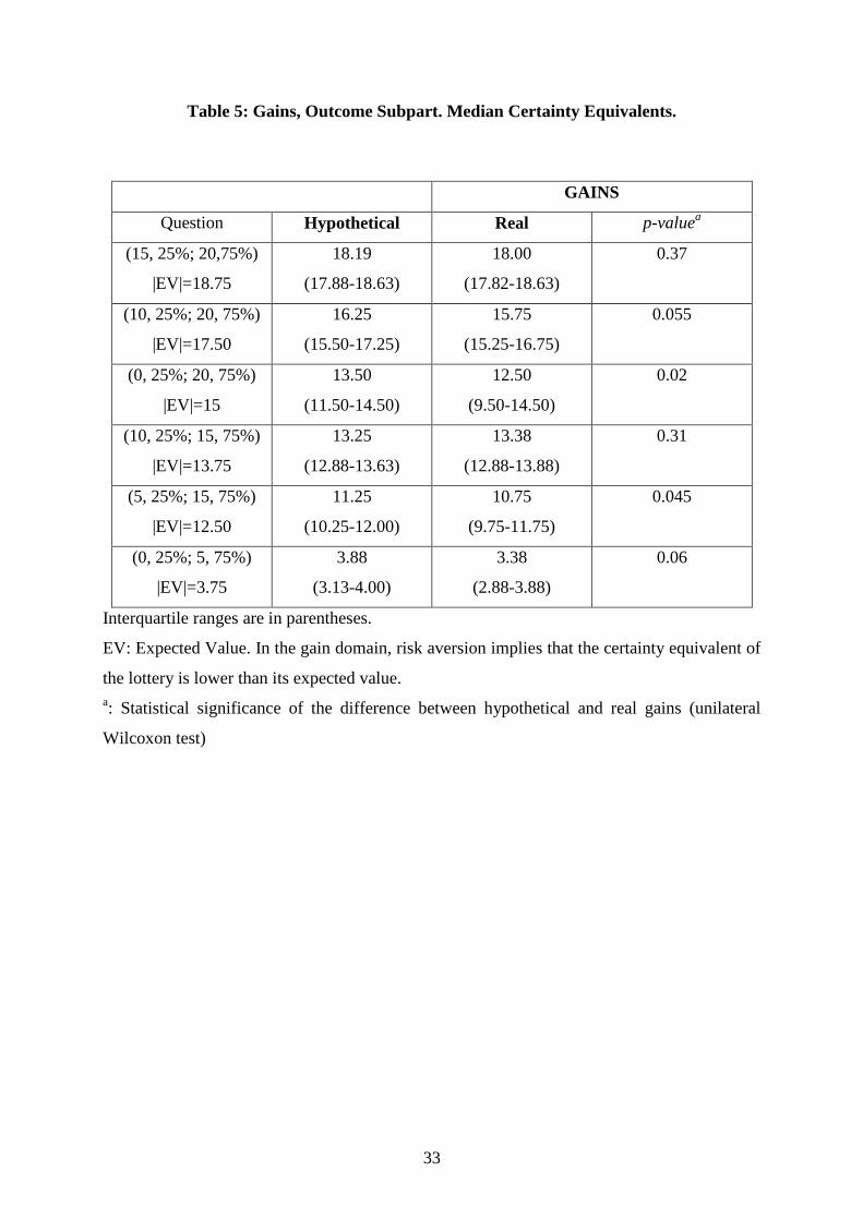
Table 5 shows the median certainty equivalents, as well as the interquartile ranges,

obtained in the outcome subpart of the gain part of the questionnaires, under both the

hypothetical gains and real gains conditions. Results are given in absolute values. In

accordance with the usual pattern of risk aversion observed when high probability-high gain

prospects are involved (remember that, in our design, the probability of the highest gain is

equal to 75%), our data offer strong evidence of risk aversion in both treatments: 11 (out of

12) median certainty equivalents are lower than the corresponding expected values.

Data from Table 5 also show that, most of the time, risk aversion is slightly stronger

when gains are real. One-tailed Wilcoxon tests show that the difference between certainty

equivalents is significant for 2 lotteries out of 6 [(0, 25%; 20, 75%), p-value: 0.02; (5, 25%;

15, 75%), p-value: 0.045] and marginally significant for two other ones [(10, 25%; 20, 75%),

p-value: 0.055; (0, 25%; 5, 75%), p-value: 0.06].14

Consequently, our data bring some support

to Assumption A3. (the hypothetical bias in the gain domain).

INSERT TABLE 5 ABOUT HERE

4.3. The Components of Risk Attitude: Utility and Probability Weighting

In order to get some deeper information about our subjects’ risk attitude in each

treatment, the utility and probability weighting functions were elicited using the semi-

parametric method developed in Abdellaoui, Bleichrodt and l’Haridon (2008). Since this

method was initially designed for the elicitation of indifferences, it was adapted to be

compatible with the multiple price list format used in this experiment, thus with a series of

14

Lottery (0, 25%; 20, 75%) offers the same specificities as the one that induced a specific behavior in the loss

domain (it offers both the worst and best possible consequences as well as, consequently, the largest spread

between consequences). The conditions under which Holt and Laury (2002)’s above-mentioned result is likely to

apply are thus satisfied. However, the other three lotteries do not share these peculiarities, so they are outside

Holt and Laury’s framework.

20

discrete choices. To be more specific, a one-parameter power specification was assumed for

the utility function u, with u(x)=x. Then, a structural maximum likelihood model was

estimated using the 6 outcome subpart certainty equivalent questions, assuming rank-

dependent utility/prospect theory preferences as well as a Fechner error specification (see

Harrison and Rutström 2008, section 3.1 for more details about structural models; Abdellaoui

et al. 2010 for a similar treatment). In the loss [resp. gain] domain, both utility parameter

and probability weight w-(0.25) [resp. w

+(0.75)] were thus estimated. Once utility was

estimated, five decision probability weights were elicited non-parametrically for each subject

on the basis of the 5 probability subpart questions, using the previously estimated value of

parameter . Aggregate results for utility (and probability weights w-(0.25) and w

+(0.75)) are

given in Table 6.15

INSERT TABLE 6 ABOUT HERE

Based on 95% confidence intervals given in Table 6, comparison of utility parameters

across the three loss treatments shows no significant difference between the hypothetical and

covered losses treatments, as well as between the covered and real losses treatments.

However, the utility function appears to be significantly more concave in the hypothetical and

covered losses treatments than in the real losses one. To be more specific, utility was found to

be convex in the real losses treatment, but convexity did actually not reach significance,

meaning that linearity could not be rejected. On the other hand, the slight pattern of concavity

observed for both hypothetical and covered losses is neither unusual in the literature

(Abdellaoui, Bleichrodt and l’Haridon 2008; Bruhin, Fehr-Duda and Epper 2010) nor

15

Note that we did not intend to estimate the entire prospect theory model here. As we did not collect any

information about the subjects’ behavior when faced with mixed prospects, we could not make any inference

about loss aversion in our experiment. As a result, our estimations were restricted to either gains or losses.

21

incompatible with rank-dependent theories such as Prospect Theory (Chateauneuf and Cohen

1994).

It was previously established that attitude toward risk did not significantly differ

between the hypothetical and real treatments in the loss domain (suggesting the absence of

any hypothetical bias). Though apparently contradictory, the significant difference in terms of

utility curvature between the hypothetical and real losses treatments may actually be

reconciled with that previous finding. It simply demonstrates that the overall no-effect of

treatment on risk attitude observed in the loss domain is actually driven by two counter-

balancing effects: on utility on the one hand, and on probabilistic risk attitude on the other

hand, as will be shown below.

As regards noise, the estimated error parameters are similar across treatments in the loss

domain, except that they are slightly higher for the covered condition. Likewise, the standard

errors are similar between the treatments.

Now, in the gain domain, no significant difference arises between the real and

hypothetical conditions, regarding either (concave) utility or error.

As regards probability weighting, five probability weights were elicited non

parametrically in each domain on the basis of the 5 probability-subpart certainty equivalent

questions, thus for p=5%, 25%, 50%, 75%, and 95%. The median probability weights and

their corresponding interquartile ranges are given in Table 7.

INSERT TABLE 7 ABOUT HERE

Once the 5 probability weights were elicited, the probability weighting function w(p)

was determined by maximum likelihood estimation, assuming a Goldstein and Einhorn (1987)

linear-in-odds two-parameter specification, with w(p)=p/(p

+(1-p)

). In this parametric

22

form, δ controls for elevation and reflects the extent to which people are attracted to

probabilistic risk, while γ governs curvature (i.e. sensitivity to probabilities, see Abdellaoui,

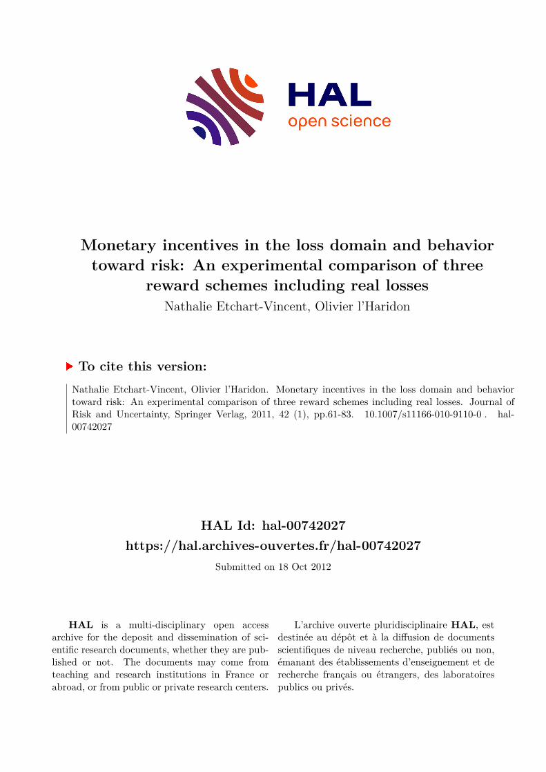
l’Haridon and Zank, 2010 for more details on these concepts). The results are shown on

Figure 1 for losses, and on Figure 2 for gains.

INSERT FIGURE 1 ABOUT HERE

Based on 95% confidence intervals, comparison of parameters δ across the three loss

treatments shows no significant difference in elevation between real, covered and hypothetical

losses. This result suggests that the degree of reality of losses at stake may not affect attitude

toward probabilistic risk. By contrast, curvature (thus sensitivity to probabilities) appeared to

be significantly lower in the real losses condition than in both the covered and hypothetical

losses conditions. This might contradict the usual claim that real choices should help

cognitive effort (which may in turn enhance sensitivity to probability).

INSERT FIGURE 2 ABOUT HERE

In the gain domain, we found a significant difference between the real and hypothetical

gains conditions for both elevation and curvature. First, as in the loss domain and quite

counter-intuitively, the real condition seemed to dampen sensitivity to probabilities. Second,

probabilistic risk seemed to be less attractive for real prospects than for their hypothetical

counterpart. In other words, real gains might induce more pessimism than hypothetical gains,

which may in turn explain why risk aversion was more prevalent when gains were real than

hypothetical (in accordance with the hypothetical bias).

23

4. Discussion

A large body of experimental literature has been devoted to the twofold question of

whether monetary incentives are actually necessary or not to collect high-quality experimental

data, and, if they may not, which reward scheme it is possible/preferable to use. Up to now,

no clear-cut or general conclusion has been drawn from these studies. However, economists

tend to consider that no appropriate behavior can be expected from the subjects unless a

performance-based payment scheme is introduced in the experimental design.

When there are losses at stake, monetary incentives are obviously hard to implement: it

is quite difficult, for ethical as well as for practical reasons, to make the subjects lose for real

by introducing a real losses payment condition (with subjects incurring some loss from their

own pocket). Consequently, it would be of great interest if some easier-to-implement reward

schemes could do as good a job as a real losses condition. In our experimental design, the idea

was to introduce a real losses condition that could be used as a benchmark to assess the

efficiency of two alternative payment schemes, namely a hypothetical losses condition, based

on a flat-fee payment, and a covered losses condition (or losses-from-an-initial-endowment

procedure), allowing the subjects to lose money from an initial endowment, but not from their

own pocket.

In the loss domain, our data suggest that few differences exist as regards behavior

between the three reward schemes under consideration. The only significant difference we

found was in utility between the real and hypothetical losses treatments. Consequently,

neither the losses-from-an-initial-endowment procedure nor the hypothetical losses procedure

seem to suffer from any expected bias. The losses-from-an-initial-endowment procedure

exhibits three features that make it a good candidate as a payment scheme in the loss domain.

First, we found no evidence for a prospect-theory-with-memory effect and only slight

24

evidence for a house money effect: as compared to the real losses treatment, the use of a

losses-from-an-initial-endowment procedure did not seem to strongly bias behavior, either

toward more risk seeking or toward more risk aversion. Second, the components of risk

attitude, utility and probability weighting, were highly similar in both the real and covered

treatments. Third, as compared to either real losses or hypothetical losses, covered losses

produced only a slightly higher amount of noise. Taken together, these findings suggest that

the losses-from-an-initial-endowment procedure, which has been widely used as a proxy to

real losses, can be considered as such and used with a high level of confidence in future

incentivized experiments involving losses.

It is of interest to observe that our data do not replicate the house money effect, which

has been well documented in the literature. A crucial difference between the seminal

experimental studies conducted by Thaler and Johnson (1990) and Battalio, Kagel and

Jiranyakul (1990) (see also Keasey and Moon, 1996) and ours is the sign of the prospects

involved in the experimental design. In Thaler and Johnson (1990)’s study for instance, the

subjects had to choose between the status-quo and a 50/50 mixed prospect; in our study, the

subjects had to choose between a sure loss and a prospect involving losses only. In the former

study, “after a gain, subsequent losses that are smaller than the original gain can be integrated

with the prior gain, mitigating the influence of loss aversion and facilitating risk-seeking”

(Thaler and Johnson, 1990, p. 657). By contrast, loss aversion played no role in our

experiment, which may have limited the increase in risk seeking expected from the house

money effect.

More boldly perhaps, our results also suggest that hypothetical losses could be

considered as an acceptable proxy for real losses. This could greatly facilitate the task of

25

experimentalists seeking to examine behavior under risk (and its components) in the loss

domain, particularly when they are limited by financial constraints.16

In the gain domain, our results look somewhat different. Indeed, hypothetical gains

appeared to induce more risk seeking among our subjects than real gains. In addition, as

compared to real ones, hypothetical choices were found to produce a larger amount of noise

as well as a more optimistic/positive attitude toward probability. Taken together, these

findings bring some support to the hypothetical bias hypothesis. Even though this support is

not very strong, it suggests that a real payment condition should be used in the gain domain.

At this stage, it is worth wondering why the impact of monetary incentives seems to

depend on the domain under consideration. It may be the case that the subjects make a strong

difference between a situation in which they hope to win real money and a situation in which

they know there is no real stake, while the prospect of losing something – be it real money,

covered or hypothetical money – is sufficiently salient and unpleasant to make the subjects

considering it as equally realistic, in a certain manner.

Of course, the initial caveat still stands: we do not claim that our results could be

directly extended outside the experimental conditions under which they were obtained (kind

of task, level of losses). In particular, it may be the case that behavior in interactive settings

involving losses, or even behavior in individual decision making settings as far as large losses

are involved, more strongly depends on the payment scheme.

16

In particular, the losses-from-an-initial-endowment procedure may induce a large cost if the subjects happen

not to lose much money from the endowment.

26

References

Abdellaoui, M. (2000). Parameter-free elicitation of utilities and probability weighting

functions. Management Science, 46, 1497–1512.

Abdellaoui, M., Baillon, A., Placido, L., Wakker P.P. (2010). The rich domain of uncertainty.

American Economic Review, forthcoming.

Abdellaoui, M., Bleichrodt, H. Paraschiv, C. (2007). Measuring loss aversion under prospect

theory: a parameter-free approach. Management Science, 53, 1659–1674.

Abdellaoui, M., Bleichrodt, H., l’Haridon, O. (2008). A tractable method to measure utility

and loss aversion in prospect theory. Journal of Risk and Uncertainty, 36, 245–266.

Abdellaoui, M., l’Haridon, O., Zank, H. (2010). Separating curvature and elevation: a

parametric weighting function. Journal of Risk and Uncertainty, 41, 39–65.

Arkes H. R., Blumer C. (1985). The psychology of sunk costs. Organizational Behavior and

Human Decision Processes, 35, 124–140.

Arkes H. R., Herren L. T., Isen A. M. (1988). The role of potential loss in the influence of

affect on risk-taking behavior. Organizational Behavior and Human Decision Processes,

42, 181–193.

Baltussen, G., Post, T., van den Assem, M. Wakker, P. (2008). The effects of random lottery

incentive schemes: Evidence from a dynamic risky choice experiment. Working Paper

Erasmus University Rotterdam.

Bardsley N. (2000) Control without deception: Individual behaviour in free-riding

experiments revisited. Experimental Economics, 3, 215–240.

Battalio, R. C., Kagel J., and Jiranyakul, K. (1990). Testing between alternative models of

choice under uncertainty: Some initial results. Journal of Risk and Uncertainty, 3(1),

25–50.

Beattie J., Loomes G. (1997). The impact of incentives upon risky choice experiments.

Journal of Risk and Uncertainty, 14, 155–168.

Becker, G. M., DeGroot, M. H., Marschak, J. (1964). Measuring utility by a single-response

sequential method. Behavioral Science, 9, 226–232.

Birnbaum, M. H. (1999). How to show that 9 > 221: Collect judgments in a between-subjects

design. Psychological Methods, 4(3), 243–249.

Bosch-Domenech A., Silvestre J. (2010). Averting risk in the face of large losses; Bernoulli

vs. Tversky and Kahneman. Economics Letters, 107(2), 180–182.

Bostic R., Herrnstein R. J., Luce R. D. (1990). The effect on the preference reversal

phenomenon of using choice indifferences. Journal of Economic Behavior and

Organization, 13, 193–212.

Bruhin, A., Fehr-Duda, H., Epper, T. (2010). Risk and rationality: Uncovering heterogeneity

in probability distortion. Econometrica, 78(4), 1375–1412.

Camerer, C. F., Hogarth, R. M. (1999). The effects of financial incentives in experiments: A

review and capital-labor-production framework. Journal of Risk and Uncertainty, 19(1),

7–42.

Chateauneuf, A., Cohen, M. (1994). Risk seeking with diminishing marginal utility in a non-

expected utility model. Journal of Risk and Uncertainty, 9, 77–91.

Clark J. (2002). House money effects in public good experiments. Experimental Economics,

5(3), 223–231.

Cox J. C., Grether D. M. (1996). The preference reversal phenomenon: Response mode,

markets and incentives. Economic Theory, 7(3), 381–405.

Cubitt R. P., Starmer C., Sugden R. (1998). On the validity of the random lottery incentive

system. Experimental Economics, 1, 115–131.

27

Davis D. D., Holt C. A. (1993). Experimental Economics. Princeton, NJ: Princeton University

Press.

Etchart-Vincent N. (2004). Is probability weighting sensitive to the magnitude of

consequences ? An experimental investigation on losses. Journal of Risk and

Uncertainty, 28(3), 217–235.

Etchart-Vincent N. (2009). Probability weighting and the ‘level’ and ‘spacing’ of outcomes:

An experimental study over losses. Journal of Risk and Uncertainty, 39(1), 45–63.

Fennema, H., van Assen, M. (1999). Measuring the utility of losses by means of the trade-off

method. Journal of Risk and Uncertainty, 17, 277–295.

Gärling T., Romanus J. (1997). Integration and segregation of prior outcomes in risky

decisions. Scandinavian Journal of Psychology, 38(4), 289–296.

Gibbons R. (1997). Incentives and careers in organizations. In D. Kreps and K. Wallis (Eds.),

Advances in economic theory and econometrics, vol. II, Cambridge, England:

Cambridge University Press.

Goldstein, W., Einhorn, H. (1987). Expression theory and the preference reversal Phenomena.

Psychological Review, 94, 236–254.

Harrison G. W. (1994). Expected utility theory and the experimentalists. Empirical

Economics, 19, 223–253.

Harrison G. W. (2006). Hypothetical bias over uncertain outcomes. In J. A. List (Ed.), Using

experimental methods in environmental and resource economics, Northampton, MA:

Elgar.

Harrison G. W. (2007). House money effects in public good experiments: Comment.

Experimental Economics, 10(4), 429–437.

Harrison G. W., Johnson E., McInnes M. M., Rutström E. E. (2005). Risk aversion and

incentive effects: Comment. American Economic Review, 95(3), 897–901.

Harrison G. W., Rutström E. E. (2008). Risk aversion in the laboratory. In N.Cox and G.W.

Harrison (Eds.), Risk aversion in experiments, Research in Experimental Economics,

12, Bingley, UK: Emerald.

Hertwig R., Ortmann A. (2001). Experimental practices in economics: A methodological

challenge for psychologists?. Behavioral and Brain Sciences, 24, 383–451.

Hertwig R., Ortmann A. (2002). Economists’ and psychologists’ experimental practices: How

they differ, Why they differ, and how they could converge. In I. Brocas and J. D. Carillo

(Eds.), The psychology of economic decisions. New York: Oxford University Press.

Holt C. A., Laury S. K. (2002). Risk aversion and incentive effects. American Economic

Review, 92, 1644–1655.

Holt, C. (1986). Preference reversals and the independance axiom. American Economic

Review, 76,508–515.

Isen A. M., Patrick R. (1983). The effect of positive feelings and risk taking: When the chips

are down. Organizational Behavior and Human Performance, 31, 194–202.

Kahneman D., Tversky A. (1979). Prospect theory: An analysis of decision under risk.

Econometrica, 47, 263–291.

Keasy K., Moon P. (1996). Gambling with the house money in capital expenditure decisions:

An Experimental Analysis. Economics Letters, 50, 105–110.

Keren, G., Raaijmakers, J. (1988). On between-Subjects versus within-Subjects comparisons

in testing utility theory. Organizational Behavior and Human Decision Process, 41, 233–

247.

Lazear E. (2000). Performance, pay and productivity. American Economic Review, 90(5),

1346–1361.

Lee, J. (2008). The effect of the background risk in a simple chance improving model. Journal

of Risk and Uncertainty, 36, 19–41.

28

Mason C. F., Shogren J. F., Settle C, List J. A. (2005) Investigating risky choices over losses

using experimental data. Journal of Risk and Uncertainty, 31(2), 187–215.

Read D. (2005). Monetary incentives, what are they good for?. Journal of Economic

Methodology, 12(2), 265–276.

Romanus J., Hassing L., Gärling T. (1996). A loss-sensitivity explanation of integration of

prior outcomes in risky decisions. Acta Psychologica, 93, 173–183.

Schoemaker, P. (1990). Are risk-attitudes related across domains and response modes?.

Management science, 36, 1451–1463.

Smith V. L. (1976). Experimental economics induced value theory. American Economic

Review, 66, 274–279.

Smith V. L., Levin I. P. (1996). Need for cognition and choice framing effects. Journal of

Behavioral Decision Making, 9, 283–290.

Starmer C., Sugden R. (1991). Does the random-lottery incentive system elicit true

preferences? An experimental investigation. American Economic Review, 81(4), 971–

978.

Stott, H. P. (2006). Cumulative prospect theory's functional menagerie. Journal of Risk and

Uncertainty, 32, 101–130.

Thaler R. H., Johnson E. J. (1990). Gambling with the house money and trying to break even:

The effects of prior outcomes on risky choice. Management Science, 36(6), 643–660.

Tversky A., Kahneman D. (1992). Advances in prospect theory: Cumulative representation of

uncertainty. Journal of Risk and Uncertainty, 5, 297–323.

Weber M., Zuchel H. (2001). How do prior outcomes affect risk attitude? Comparing

escalation of commitment and the house-money effect. Decision Analysis, 2(1), 30–43.

29

Table 1: The Five Payment Conditions and the Four Tested Assumptions.

Hypo. losses

Real losses

Real gains

Covered

losses

House money effect

(A1.1.)

House money effect

(A1.1.)

Prospect-theory-with-

memory effect

(A1.2.)

Prospect-theory-with-

memory effect and

recoding

(A1.2a)

Hypo.

losses

Hypothetical bias for

losses

(A2.)

Hypo.

gains

Hypothetical bias

for gains

(A3.)

Hypo.: Hypothetical

a: Comparison between real gains and “recoded” covered losses

30

Table 2: The Stimuli.

Loss part Gain part

Outcome

subparta

(-20, p; 0, 1-p)

(-10, p; 0, 1-p)

(-5, p; 0, 1-p)

(-10, p; -5, 1-p)

(-20, p; -15, 1-p)

(-15, p; -5, 1-p)

with p = 25%

(20, 1-p; 0, p)

(20, 1-p; 10, p)

(20, 1-p; 15, p)

(15, 1-p; 10, p)

(5, 1-p; 0, p)

(15, 1-p; 5, p)

with 1-p = 75%

Probability

subpartb

(-20, p; 0, 1-p)

with p = 5%, 25%, 50%, 75%, 95%

(20, 1-p; 0, p)

with 1-p = 5%, 25%, 50%, 75%, 95%

+ Additional lottery (60, 5%; 0, 95%)

a: The probabilities are held constant in the prospects, only the outcomes vary.

b: The outcomes are held constant in the prospects, only the probabilities vary.

31

Table 3: Equality of Risk Premia Between Treatments (ANOVA tests).

Hypo. Losses

Real losses

Real gains

Covered

losses

House money effect (A1.1.)

Equality of risk premia not

rejected (p=0.66)

House money effect (A1.1.)

&

Prospect-Theory-with-

memory effect (A1.2.)

Equality of risk premia not

rejected (p=0.25)

Prospect-theory-with-

memory effect and recoding

(A1.2a)

Equality of risk premia

rejected (p=0.002a)

Hypo.

losses

Hypothetical bias

for losses (A2.)

Equality of risk premia not

rejected (p=0.25)

Hypo.

gains

Hypothetical bias

for gains (A3.)

Equality of risk premia

rejected (p=0.01)

Factorial repeated measures ANOVA on risk premia with three between-subject factors

(gender, lottery order and gain/loss order) and two within-subject factors (lottery, session).

The risk premium is defined as the difference between the certainty equivalent and the

expected value of the lottery.

The hypothesis under investigation holds if the equality of risk premia is rejected.

Hypo.: Hypothetical

a: Comparison between real gains and “recoded” covered losses

32

Table 4: Losses, Outcome Subpart. Median Certainty Equivalents (absolute values).

LOSSES

Question Hypothetical Real Covered p-valuea

(-5, 25%; 0, 75%)

|EV|=1.25

1.38

(1.13-2.00)

1.63

(1.13-2.13)

1.50

(1.13-2.13)

0.92

(-10, 25%; 0, 75%)

|EV|=2.5

3.25

(2.75-4.25)

3.25

(2.75-3.75)

3.25

(2.75-3.75)

0.95

(-20, 25%; 0, 75%)

|EV|=5

7.50

(5.50-7.50)

5.50

(5.50-7.50)

6.50

(5.50-7.50)

0.24

(-10, 25%; -5, 75%)

|EV|=6.25

6.50

(6.13-7.13)

6.63

(6.13-6.88)

6.63

(6.13-6.63)

0.77

(-15, 25%; -5, 75%)

|EV|=7.50

8.19

(7.25-8.75)

8.25

(7.25-8.75)

8.00

(7.25-8.75)

0.56

(-20, 25%; -15, 75%)

|EV|=16.25

16.44

(16.13-17.13)

16.63

(16.13-16.88)

16.63

(16.13-17.13)

0.46

Interquartile ranges are in parentheses.

EV: Expected Value. In the loss domain, risk aversion implies that, in absolute value, the

certainty equivalent of the lottery is higher than its expected value.

a: Statistical significance of the difference between real, hypothetical and covered losses

(Friedman test)

33

Table 5: Gains, Outcome Subpart. Median Certainty Equivalents.

GAINS

Question Hypothetical Real p-valuea

(15, 25%; 20,75%)

|EV|=18.75

18.19

(17.88-18.63)

18.00

(17.82-18.63)

0.37

(10, 25%; 20, 75%)

|EV|=17.50

16.25

(15.50-17.25)

15.75

(15.25-16.75)

0.055

(0, 25%; 20, 75%)

|EV|=15

13.50

(11.50-14.50)

12.50

(9.50-14.50)

0.02

(10, 25%; 15, 75%)

|EV|=13.75

13.25

(12.88-13.63)

13.38

(12.88-13.88)

0.31

(5, 25%; 15, 75%)

|EV|=12.50

11.25

(10.25-12.00)

10.75

(9.75-11.75)

0.045

(0, 25%; 5, 75%)

|EV|=3.75

3.88

(3.13-4.00)

3.38

(2.88-3.88)

0.06

Interquartile ranges are in parentheses.

EV: Expected Value. In the gain domain, risk aversion implies that the certainty equivalent of

the lottery is lower than its expected value.

a: Statistical significance of the difference between hypothetical and real gains (unilateral

Wilcoxon test)

34

Table 6: Estimation Results, Utility

LOSSES GAINS

Hypothetical Real Covered Hypothetical Real

Utility

parameter

1.09

(1.05-1.13)

0.99

(0.95-1.03)

1.06

(1.02-1.11)

0.96

(0.90-1.00)

0.95

(0.91-1.00)

Error

parameter

0.048

(0.046-0.051)

0.046

(0.044-0.048)

0.052

(0.049-0.054)

0.069

(0.066-0.072)

0.060

(0.058-0.064)

Probability

weighta

0.305

(0.297-0.313)

0.317

(0.309-0.325)

0.322

(0.313-0.330)

0.647

(0.638-0.656)

0.61

(0.603-0.620)

95% confidence intervals are in parentheses.

a: w

-(0.25) for losses and w

+(0.75) for gains.

Table 7: Estimation Results, Probability Weights

LOSSES GAINS

Hypothetical Real Covered Hypothetical Real

p=5% 0.103

(0.06-0.19)

0.177

(0.13-0.22)

0.155

(0.11-0.20)

0.239

(0.08-0.34)

0.214

(0.14-0.29)

p=25% 0.292

(0.24-0.34)

0.327

(0.28-0.43)

0.301

(0.25-0.35)

0.340

(0.24-0.49)

0.291

(0.24-0.39)

p=50% 0.494

(0.39-0.55)

0.467

(0.38-0.53)

0.502

(0.40-0.55)

0.489

(0.39-0.64)

0.490

(0.34-0.54)

p=75% 0.651

(0.55-0.76)

0.626

(0.53-0.73)

0.657

(0.60-0.76)

0.735

(0.59-0.78)

0.638

(0.54-0.73)

p=95% 0.757

(0.70-0.86)

0.776

(0.72-0.83)

0.814

(0.71-0.87)

0.879

(0.73-0.93)

0.832

(0.74-0.93)

Interquartile ranges are in parentheses.

35

Figure 1: Estimation Results, Probability Weighting Functions, Losses

36

Figure 2: Estimation Results, Probability Weighting Functions, Gains

37

Appendix A: A Typical Choice Situation

38

Appendix B: The Recoding Mechanism used for Building Each Gain Lottery

To allow the testing of Assumption A1.2., the gain gambles had to be built from the loss ones

using the following mechanism. Suppose that we use a losses-from-an-initial-endowment

procedure with an initial endowment of A > 0. Now, consider a subject who is tempted to deal

with covered losses as if they were real gains by integrating the initial endowment A into the

subsequent losses she may undergo. As a result, when faced with the covered losses prospect

P- = (X, p; Y, 1-p) [with –A < X < Y < 0], she may behave as if she were actually confronting

the positive prospect P+ = (X + A, p; Y + A, 1-p) [with 0 < X + A < Y + A < A.]. This “as if”

(AI) Lottery P+ is denoted PAI

+. Now, let us denote CE

- the certainty equivalent of the subject

for P-, and CEAI

+ her “as if” certainty equivalent for PAI

+. CEAI

+ is thus given by CEAI

+ = CE

-

+ A. Note that the first formula assumes that the initial endowment is completely integrated

into subsequent losses. If the integration process is only partial, CEAI+ will be given by CEAI

+

= CE- + B, with 0 < B < A.

From an empirical point of view, we obviously can not observe whether a subject integrates

her initial endowment into subsequent losses (be it partially or completely) or not.

Nevertheless, we can in fact determine whether she does or not (and test Assumption A1.2.),

by comparing her behavior in the covered losses condition, after recoding these losses as

gains by integrating the initial endowment into subsequent losses, and her behavior in the

corresponding real gains condition. More specifically, all we have to do is compare her “as if”

certainty equivalent for PAI+, namely CEAI

+, with her certainty equivalent when facing the

same lottery P+ but under a “real gains” (R) condition, denoted CER

+.

To permit such a comparison, each of the 11 gain prospects P+ has to be built as the positive

counterpart of one of the 11 initial loss prospects P- = (X, p; Y, 1-p), using the simple formula

P+ = (X + A, p; Y + A, 1-p) where A is the initial endowment.