Monetary Policy Alternatives at the Zero Bound:

Lessons from the 1930s U.S.

March, 2013

Christopher HanesDepartment of Economics

State University of New York at BinghamtonP.O. Box 6000

Binghamton, NY 13902(607) 777-2572

chanes@binghamton.edu

Abstract: In recent years economists have debated two unconventional policy options forsituations when overnight rates are at the zero bound: boosting expected inflation throughannounced changes in policy objectives such as adoption of price-level or nominal GDP targets;and LSAPs to lower long-term rates by pushing down term or risk premiums - “portfolio-balance” effects. American policies in the 1930s, when American overnight rates were at the zerobound, created experiments that tested the effectiveness of the expected-inflation option, and theexistence of portfolio-balance effects. In data from the 1930s, I find strong evidence of portfolio-balance effects but no clear evidence of the expected-inflation channel.

For comments and suggestions, thanks to William English, John Fernald, James Hamilton, BarryJones, Edward Nelson, Gary Richardson, Eric Swanson, Susan Wolcott and Wei Xiao; and toparticipants in the Federal Reserve Bank of San Francisco conference “The Past and Future ofMonetary Policy,” March 2013.

1Here and elsewhere I use the term “liquidity trap” in the most conventional way, to mean that the short-term rate is at its lower bound.

2“Quantitative easing” is sometimes used more specifically to mean operations that exchange long-term

assets for reserve balances (not short-term assets).

1

In recent years economists have considered two “unconventional” monetary policy

options as last resorts for situations when real activity is too low, but the central bank has already

pushed the overnight rate to the zero bound and done its best to convince the public the overnight

rate will remain zero for a long time - “forward guidance.” One is to announce a credible change

in policy objectives that raises the inflation rate the public expects the central bank to aim for in

the future, when the economy is out of the liquidity trap and conventional tools work again.1 An

increase in the central bank’s inflation target would do the trick. So would the replacement of an

inflation target with a target for the path of the price level or nominal GDP: these imply inflation

must be temporarily high at some point in the future to make up for current shortfalls. Another

option is for the central bank to acquire long-term bonds in open-market operations, in exchange

for newly-created reserve balances or short-term bonds from the central bank’s portfolio. Such

operations are often referred to loosely as “quantitative easing.”2 Federal Reserve policymakers

call them “large-scale asset-purchase” programs or LSAPs.

A credible change in policy objectives could work partly as another form of forward

guidance, through rational expectations of financial-market participants. If they become more

convinced the central bank will choose low short-term interest rates in the post-trap future,

current long-term rates may fall somewhat. However, in conventional New Keynesian models a

bigger bang comes through rational expectations of agents participating in the wage- and price-

setting process. In the “new Keynesian Phillips curve,” current inflation is affected by levels of

inflation and real activity expected to prevail at distant horizons. To the degree that a change in

objectives implies higher inflation for the post-trap future, it raises inflation immediately, even

while short-term rates remain stuck at the zero bound. That reduces real interest rates, boosts

spending and can lift the economy out of the liquidity trap by its expectational bootstraps

3It is not necessarily linked to any observable current action. It may be time-inconsistent: in a recoveredeconomy, it would be better to return to the old inflation target, which presumably reflected underlyingpreferences (Eggertsson and Woodford, 2003; Adam and Billi, 2007).

2

(Krugman, 1998; Woodford, 2012).

Policymakers have not tried the expected-inflation mechanism in recent years, despite its

theoretical appeal. Perhaps they doubt it would work in reality. Many empirical studies find the

new Keynesian Phillips curve fits the data only if one assumes expectations are less rational than

in standard models (Roberts, 1997; Ball, 2000; Rudd and Whelan, 2007; Fuhrer, 2012). Even if

expectations are rational, it may be hard for policymakers to make the new objective credible.3

To improve credibility, Lars Svensson recommends a policy package he calls the “Foolproof

Way” out of a liquidity trap. A key element is a peg to a depreciated exchange rate, which

“serves as a conspicuous commitment to a higher price level in the future” (2003, p. 155).

LSAPs, like a change in policy objectives, might lower long-term rates somewhat just by

reinforcing the message that overnight rates will remain zero for a long time. During a financial

crisis, LSAPs in disrupted markets can lower rates by reducing liquidity premiums (a form of

“credit easing”). But most advocates of LSAPs hope they can lower long-term rates in well-

functioning markets by pushing down on term or risk premiums - other “portfolio-balance”

effects. As a matter of theory portfolio-balance effects are trickier than the expected-inflation

mechanism. They do not exist at all in many economists’ preferred models (Woodford, 2012).

Despite their theoretical shortcomings, LSAPs have been tried by the Federal Reserve and

other central banks in the zero-bound era since 2008. The Fed’s “Operation Twist” of 1961 was

an LSAP: though the U.S. was not at the zero bound, the Fed bought long-term Treasuries (in an

attempt to lower long-term rates and stimulate real activity) while selling short-term Treasuries

(to raise short-term rates and improve the balance of payments). Some Bank of Japan (BOJ)

“quantitative easing” operations in the early 2000s, when Japan was at the zero bound, were also

4Not all. Some BOJ operations exchanged reserves for short-term assets with yields already practicallyzero (Gagnon, Raskin, Remache and Sack, 2011 p. 36; Ueda 2012). Everyone agrees that exchangingreserves for assets currently paying zero interest will have no effect on market yields even if there is aportfolio-balance channel (Hamilton and Wu 2012; Woodford 2012, p. 60).

3

LSAPs.4

Empirical studies have looked for effects of Operation Twist (Swanson, 2011), BOJ

operations (Bernanke, Reinhart and Sack, 2004; Ueda, 2012) and post-2008 LSAPs by the Fed

(Neely, 2012; Gagnon, Raskin, Remache and Sack, 2011; Krishnamurthy and Vissing-Jorgensen

2011; D’Amico, English, Lopez-Salido and Nelson, 2012) and the Bank of England (Joyce,

Lasaosa, Stevens and Tong 2011). Most conclude these operations (with the possible exception

of the BOJ’s) did tend to lower long-term rates. But it is not generally agreed they did so through

a portfolio-balance channel. A big problem is that the intent and timing of all these operations

were well-publicized. Whether or not a portfolio channel actually exists, financial-market

participants would presumably price in the possibility the LSAPs would work: there was

practically no experience on which to base a reliable forecast they would fail (Reichlin, 2011, p.

192; Krishnamurthy and Vissing-Jorgensen discussion p. 280). That would create a temporary

effect on term premiums. Indeed, some studies find that the apparent effects of the operations

disappeared quickly (Wright, 2012; Neely, 2012, p. 27; Woodford, 2012 p. 71). Also, news about

the operations may have changed market participants’ expectations of future overnight rates by

signalling something about policymakers’ preferences or private information (Cochrane, 2011, p.

4; Woodford, 2012, p. 57, 72) - the “signalling channel.” Some studies try to parse out the

contributions of the signalling channel versus changes in term premiums with estimated dynamic

term-structure models. Such models necessarily assume expectations of future overnight rates

can be inferred from statistical relationships in data from periods when the overnight rate was

positive. Unfortunately, it is not clear that key patterns remain the same when the overnight rate

is zero (Bauer and Rudebusch, 2012, Woodford, 2012 p. 78). To generalize, within a model one

can work out the correspondence between relationships observed to hold in ordinary times, and

4

relationships that hold in the extraordinary conditions of the zero bound. In the absence of an

agreed-upon model there may be special value to evidence drawn from periods when the

economy was actually in a liquidity trap.

The American economy has been in a liquidity trap once before, in the 1930s. Across the

downturn of the Great Depression, from 1929 to early 1933, interest rates in America’s formerly

active overnight-lending markets fell to practically zero. According to Krugman (1998, p. 137),

American interest rates were “hard up against the zero constraint.” They remained there for the

rest of the decade. Meanwhile, American policies tested the practical effectiveness of the

expected-inflation option: over 1933 the incoming Roosevelt administration devalued the dollar

as part of an announced policy to inflate the overall price level. Policy also created natural

experiments testing the existence of portfolio effects. Over 1934-36, the interaction of Treasury

and Federal Reserve practices created variations in asset supply relevant for some types of

portfolio effects, specifically those due to investors’ avoidance of duration (or interest-rate) risk.

Importantly, these events were accidental and unpublicized (like the accidental reserve-supply

shocks studied by Hamilton [1997] and Carpenter and Demiralp [2006]). Policymakers did not

claim they would affect bond prices, and their exact timing was unknown to market participants.

In this paper, I examine the results of both sets of experiments.

I begin by describing exchange-rate and monetary policies over the 1930s and interpreting

them in terms of open-economy Keynesian models. Next, I look for evidence that devaluation

and pro-inflation announcements over 1933-34 and monetary policy turns later in the 1930s

affected inflation through long-term expectations. I find only very ambiguous evidence. Over

1933-34 there was a sharp pickup in inflation that cannot be accounted for by the usual Phillips-

curve relation with real activity, or by direct effects of devaluation. But there is a good alternative

explanation for these inflation anomalies: changes in labor markets that were, in the language of

DSGE models, “markup shocks.” Over 1933-34, the National Recovery Administration (NRA)

fixed minimum wages by industry, banned wage cuts, encouraged union formation and

5

strengthened union bargaining power. When the NRA was declared unconstitutional in 1935,

many of its pro-union and wage-fixing policies were maintained in other forms. There is no

reliable way to calibrate or estimate from another era the magnitude of these mark-up shocks. I

cannot rule out that inflation was boosted by both markup shocks and an increase in expected

future inflation. But the exact timing of the inflation anomalies is entirely consistent with the

operation of the NRA and unionization.

Finally, I examine data from 1934-36 to see whether accidental fluctuations in asset

supply affected bond yields as predicted by a duration-risk view of portfolio-balance effects. I

find strong evidence they did.

1) Exchange-rate and monetary policies over the 1930s

The late 1920s

In the late 1920s the shortest maturity of lending in the United States was overnight.

Overnight instruments included fed funds loans (loans between firms with accounts in the

Federal Reserve system, usually without collateral); repurchase agreements (repos) on federal

securities; “call money” or “brokers’ loans” collateralized by stocks and bonds traded on New

York exchanges; and interest-paying interbank deposits (Haney, Logan and Gavens 1932; United

States Senate 1931 part 1, 1048; Turner 1931).

The U.S. and most of its international trading partners were in an international gold

standard system. Monetary authorities exchanged currency and central bank reserve deposits for a

fixed quantity of gold, effectively fixing international exchange rates. Authorities covered

deficits in the balance of payments with outflows of monetary gold and/or sales of official

foreign-asset reserves. Authorities facing a persistent balance-of-payments deficit would

eventually have to raise local interest rates, depressing real activity. The resulting capital inflows

and decrease in imports would improve the balance in the short run. In the long run, the

disinflation or deflation associated with depressed real activity would decrease the country’s

relative wage and price level, devaluing its real exchange rate. A country with a balance-of-

6

payments surplus was supposed to do the opposite, according to the gold standard’s “rules of the

game.” In their classic form, the rules barred persistent accumulation of foreign reserves or

sterilization of gold inflows so that a balance-of-payments surplus would automatically boost its

high-powered money supply and hence reduce its short-term interest rates. Ultimately, a

country’s long-run price level would be determined by its currency’s gold content and the gold

price level of tradable goods. The gold price level depended in turn on the balance of world gold

supply against gold standard countries’demand for gold reserves (as distinct from reserves of

foreign assets). In the United States, most economists and writers in business publications

thought about the price level in these terms. They assumed the dollar’s gold value would remain

fixed and forecast a stable or slightly decreasing price level based on the balance of world gold

supply and demand (Nelson, 1991: 6-7).

In fact, many countries with persistent balance-of-payments surpluses accumulated

reserves of foreign assets or increased gold reserves rather than allow domestic inflation to take

place. One of these was the U.S. In the late 1920s the Federal Reserve system was in charge of

America’s gold reserves as well as domestic monetary policy. Fed staff monitored measures of

domestic prices and economic activity. In decisions about discount rates and open-market

operations, Fed policymakers aimed to keep inflation low, stabilize output and forestall financial-

market bubbles. This usually required them to sterilize gold inflows and accumulate reserves

(Meltzer, 2003: 169,209,230). Fed policymakers did not have a shared, coherent view of

monetary policy, but one could argue they followed the Taylor rule rather than the gold-standard

rules of the game (Orphanides, 2003). It is not clear what they would have done in the end if the

Great Depression had not occurred. Presumably they would not have been willing to keep

accumulating gold and foreign assets forever. That could mean they would have ultimately

allowed inflation to take place in the U.S. But the imbalance could also have been resolved by

forcing other countries, losing gold, to deflate.

The Great Depression and the onset of the liquidity trap

5It was not unheard of for stock-exchange authorities to deliberately set the official call-money rate

above the market-clearing level: they had done this at times prior to 1932 (Beckhart 1932: 55).

7

In response to the October 1929 stock market crash the Federal Reserve system cut

discount rates, purchased Treasury bonds in open-market operations and refrained from

sterilizing gold inflows. Fed funds and call money rates declined sharply, rose for a while in late

1931 as the Fed tightened in the wake of Britain’s devaluation, then fell further. By late 1932 fed

funds rates were as low as 13 basis points (Turner, 1931:47). As one would expect, the wave of

bank panics that culminated in the national bank holiday of March 1933 shut down the fed funds

market due to default fears. By early 1934 confidence in banks had been restored by steps such as

the introduction of Federal deposit insurance: deposits flooded back into banks; bank stock and

debt prices recovered. But the fed funds market did not revive: “there were practically no

occasions when there were borrowers in need” (Willis 1957:11) The repo market was likewise

moribund; the rate on interbank deposits at New York money center banks was cut to zero by

early 1933, prior to the regulatory prohibition of interest on such deposits (Bradford, 1941: 445;

Federal Reserve Board 1934: 629, 1936: 31; Homer, 1963: 376).The call money market had

continued to function through the October 1929 stock crash (haircuts on collateral value were

more than sufficient to protect lenders [Bradford 1941: 444]), but call money rates fell along with

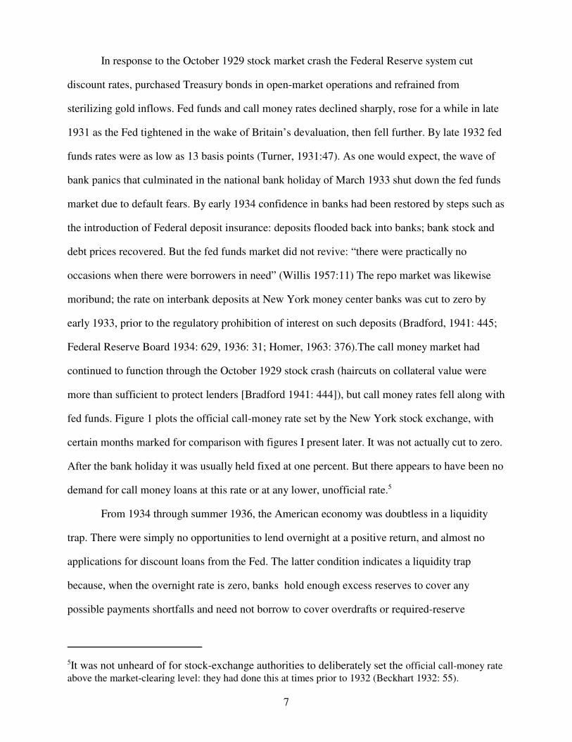
fed funds. Figure 1 plots the official call-money rate set by the New York stock exchange, with

certain months marked for comparison with figures I present later. It was not actually cut to zero.

After the bank holiday it was usually held fixed at one percent. But there appears to have been no

demand for call money loans at this rate or at any lower, unofficial rate.5

From 1934 through summer 1936, the American economy was doubtless in a liquidity

trap. There were simply no opportunities to lend overnight at a positive return, and almost no

applications for discount loans from the Fed. The latter condition indicates a liquidity trap

because, when the overnight rate is zero, banks hold enough excess reserves to cover any

possible payments shortfalls and need not borrow to cover overdrafts or required-reserve

6The maturity of newly-issued Treasury bills varied over the 1930s and discount rates on newly-issuedbills were sometimes negative for well-understood reasons. The figure plots estimates of three-monthyields that control for these factors, from Cecchetti (1988).

8

deficiencies (Hanes, 2006). Treasury yields, also plotted in Figure 1, were extremely low but not

as low as after 2008.6 Three-month Treasuries were usually less than a quarter of a percent, but

bond yields remained above 2 1/2 percent. Relative to the post-2008 period, financial-market

participants may have placed a higher probability on a faster “lift-off” from the zero bound.

In the outside world, gold demand had increased sharply after 1929 due to widespread

runs on banks and currencies. In any gold-standard country, output and employment could

remain at the natural rate only if there was a massive deflation of wages and prices, or a

devaluation of the currency relative to gold (Temin, 1989; Eichengreen, 1992; Bernanke, 1995;

Bernanke and Mihov, 2000). Most countries eventually chose the latter, but only after suffering

the former. Some, including France and the Netherlands, held to their 1929 gold values until

autumn 1936 (Clarke, 1977; Eichengreen and Sachs, 1985). The resulting monetary regime was

not like the recent era of floating exchange rates. It was more like the Bretton Woods system with

a much smaller role for dollars. Major countries pegged against gold, or managed their currency’s

gold exchange rate within a tight band (e.g. Britain). Many countries (e.g. Germany) adopted

exchange controls.

American policy 1933-39

Coming out of the Bank Holiday, in April 1933 the new Roosevelt administration ordered

the Treasury and banks to cease paying out gold for currency and deposits, ordered Americans to

sell privately held monetary gold to the government, and allowed the dollar to float against gold

in foreign markets. In June 1933 Congress passed legislation abrogating financial contracts that

required payment in gold at the old parity, and Roosevelt sent representatives to an international

economic conference in London. The London conference was aimed at restoration of gold

convertibility at the old exchange rates. But “while it was in process, the President apparently

decided definitely to adopt the path of currency depreciation” (Friedman and Schwartz, 1963:

7In his second “fireside chat” on May 7th, Roosevelt said “The Administration has the definite objectiveof raising commodity prices to such an extent that those who have borrowed money will, on the average,be able to repay that money in the same kind of dollar which they borrowed.”

8On October 22: “I repeat what I have said on many occasions, that the definite policy of the Government

has been to restore commodity price levels. The object has been the attainment of such a level as will

enable agriculture and industry once more to give work to the unemployed. It has been to make possible

the payment of public and private debts more nearly at the price level at which they were incurred. It has

been gradually to restore a balance in the price structure so that farmers may exchange their products for

the products of industry on a fairer exchange basis. It has been and is also the purpose the prevent prices

from rising beyond the point necessary to attain those ends...Obviously..we cannot reach the goal in only

a few months. We may take one year or two years or three years...When we have restored the price level,

we shall seek to establish and maintain a dollar which will not change its purchasing and debt paying

power during the succeeding generation.”

9

469). At the beginning of July, he sent a message to the conference disavowing its aims. In

January 1934, the Gold Reserve Act fixed a new gold value for the dollar, depreciated about 40

percent from its pre-1933 value. Over January and February 1934 Treasury purchases of gold in

foreign markets drove the dollar down to the new rate. The dollar was not devalued again in the

1930s (and for a long time afterwards) but at times another devaluation was widely viewed as

possible (Clarke, 1977: 11). The gold value fixed the dollar’s exchange rate against countries that

were holding to their 1929 gold values, such as France. Through early 1938 the dollar’s exchange

rate also remained within a tight range against sterling and the countries of the British Empire

that pegged to sterling.

Dollar devaluation was part of an announced policy to raise the overall price level,

supported by Roosevelt and many congressmen. In May 1933 Roosevelt began to state clearly

that his administration intended to “reflate” prices to their pre-Depression level, and Congress

passed the Thomas amendment to the Agricultural Adjustment Act, which was “explicitly

directed at achieving a price rise through expansion of the money stock” (Friedman and

Schwartz, 1963, p. 465).7 In a fireside chat of late October 1933, Roosevelt gave perhaps his

most explicit and detailed statement of support for future inflation.8 Roosevelt and other

supporters of reflation believed (or at least hoped) it would promote economic recovery, but it is

9Roosevelt took counsel from many economists and financiers. Some strenuously opposed devaluationand reflation. Roosevelt’s actions were most consistent with the ideas of Cornell economist George F.Warren. Warren understood that under a gold standard each country’s price level was determined by itscurrency’s gold value, and that prices of internationally-traded agricultural commodities were set inworld markets so their prices in any one country would respond immediately to a change in thecurrency’s gold value (Warren and Pearson, 1933). He believed that the structure of relative prices hadbeen disturbed after 1929, because prices of internationally traded agricultural commodities hadplummeted but “sticky” prices of domestic manufactured goods had not. In the words of Warren’scolleague and co-author, Frank Pearson (1957, p. 5671), “The problem..was to deflate the high, sticky

prices down to the level of the low, flexible prices or to inflate the low, flexible prices up to the high,

sticky prices. There was no other alternative..F.D.R. had plenty of advice on what should be done. One

group proposed that the process of deflation should be completed; their remedy, completion of deflation,

would have been politically unacceptable. Dr. Warren had the correct remedy: the equilibrium should be

restored by inflating the flexible relative to the sticky prices by raising the [dollar currency] price of

gold.”

10In this era, railroad managers’ associations surveyed freight customers on a quarterly basis to get theirplans for rail shipments in the upcoming quarter. Customers reported their planned volumes of shipmentfor the next quarter as percent increases over the same quarter in the previous year. Suitably aggregatedreports from manufacturing firms, given by Hart (1960), indicate their production plans for the upcomingquarter. Since early 1929, manufacters’ production plans for coming quarters had embodied decreases inplanned output from the same quarter of the previous year (and realized output had always been evenlower than planned). Starting in the first quarter of 1933, manufacturers began to plan increases inproduction over the previous year. See especially Chart 2, p. 210.

10

not clear what channel they had in mind.9

Figure 2 plots dollar exchange rates against sterling and the French franc from 1932

through 1937. The dollar had already depreciated substantially prior to FDR’s disavowal of the

London economic conference in July 1933. Figure 3 shows that the changing rate was

immediately reflected in domestic prices of raw commodities traded on international competitive

markets, such as cotton (a U.S. export) and rubber (an import). A price index from the era that

covers a wide set of raw materials used by industry, weighted by values of domestic

consumption, also shows a strong, immediate effect of devaluation.

Real activity, meanwhile, turned up from a trough in March 1933 according to the

NBER’s chronology. The upturn appears in the FRB’s IP index, plotted in Figure 4 with a

measure of unemployment I will explain later. The turnaround was perceived at the time.

Businessmen expected it to continue.10

From 1934 through the end of the 1930s the U.S. usually ran a balance of payments

11Reputable professional economists have expressed similar fears about the post-2008 buildup of excessreserves, e.g. Martin Feldstein in the Wall Street Journal (January 3, 2013): “Because of the Fed’spurchases of bonds and mortgage-backed securities, commercial banks have $1.4 trillion more in reservesthan is legally required by the size of their balance sheets. The banks can use these excess reserves tocreate loans and deposits, which will increase the money supply and fuel inflation...the day will comewhen aggregate demand is increasing, companies want to borrow, and the banks are willing to lendaggressively.” In the 1930s such fears were perhaps not unreasonable as the Fed had no notion of payinginterest on reserves, and given the lack of knowledge at the time about the monetary transmissionmechanism and the Phillips curve.

11

surplus and accumulated monetary gold, as it had in the 1920s. Under new institutional

arrangements gold was purchased from foreign sellers by the Treasury rather than the Fed. The

Treasury also bought gold and silver from domestic mines. Through summer 1936, American

policymakers allowed these specie purchases to boost the high-powered money supply. A

Treasury gold purchase added to the money supply when the Treasury created a gold certificate

“backed” by the purchased gold, deposited the certificate in its account at the Fed, and made

payments out of its Fed account or transferred funds from its Fed account to Treasury accounts in

commercial banks. The Fed did not sterilize effects of Treasury specie purchases. In fact it did

not engage in open-market operations at all except to replace maturing securities in its portfolio

(Friedman and Schwartz 1963: 511). As the economy recovered, some high-powered money

growth went to accommodate increasing demand for currency, but most went into banks’ excess

reserves. This is apparent in Figure 5, which plots the American monetary gold stock (held by the

Treasury), the high-powered money supply (currency held by the public plus nonborrowed

reserves) and nonborrowed reserves from April 1934 on. From January 1934 to December 1936

the high-powered money supply increased about 63 percent. Nonborrowed reserves increased

more than 85 percent.

In 1936 Federal Reserve policymakers began to push for a hike in reserve requirements to

soak up excess reserves. They feared that the buildup of excess reserves could allow a burst of

uncontrollable inflation to take place in the future.11 They did not believe a hike in reserve

requirements would have any immediate effect on interest rates, bank lending or real activity

12

(Goldenweiser 1951: 175-82). In July 1936 the Fed announced a hike to take effect in August.

Though the move had been negotiated with the Treasury, Treasury officials were not expecting

the announcement to take place on the day it did (Blum, 1959:356; Meltzer 2003: 503). In

January 1937 the Fed announced that more hikes in reserve requirements would occur in March

and May 1937. Meanwhile, in December 1936 the Treasury announced it would sterilize gold

inflows. It began to do so immediately, by refraining from the creation of gold certificates against

purchased gold. In effect, the Treasury began to pay for gold with additional Treasury borrowing

rather than high-powered money creation. “Inactive” gold was counted part of the U.S. gold

stock but not the high-powered money supply. As a matter of government accouting it was an

addition to “Treasury cash” - funds credited to the Treasury but held neither in the Fed nor

commercial bank accounts. The cessation of money growth and buildup in Treasury cash is

obvious in Figure 5, which plots the sum of Treasury cash and Treasury Federal Reserve

accounts.

According to the NBER chronology, the economy entered a recession in May 1937. Fed

and Treasury officials had observed signs of a slowdown in economic growth before that. In

response, they began to reverse their earlier actions. In March 1937 the Treasury bought bonds;

in April the Fed announced that, for the first time since 1933, it would buy bonds to boost reserve

supply (Blum 1959: 269-375; Gordon and Westcott 1937: 107). In September 1937 the Fed

announced more bond purchases “for the continuation of the System’s policy of monetary ease”

(Blum, 1959: 378) and the Treasury announced it would boost the money supply by creating gold

certificates against part of its stock of inactive gold (Johnson 1939: 137). In February 1938 the

Treasury announced that a limited volume of current gold purchases would be allowed to boost

the money supply (Crum, Gordon and Westcott 1938b: 93). In April 1938 FDR announced that

all inactive gold and all future gold inflows would be released into the money supply, and reserve

requirements would be reduced immediately (Crum, Gordon and Westcott 1938b:94; Blum

1959:425).

13

2) The expected-inflation channel and 1930s policies

2.1) Theory

Roosevelt’s policy package of 1933-34 bears obvious similarities to Svennson’s

Foolproof Way out of a liquidity trap. Krugman (1998, p. 161), and Svensson (2004, p. 90)

speculate that the Roosevelt administration’s policies constituted an example of the expected-

inflation option. Temin and Wigmore (1990, p. 485) argue that “The devaluation of the dollar

was the single biggest signal” of a change in regime; “Devaluation...sent a general message to all

industries because it marked a change in direction for government policies and for prices in

general” (p. 485). Romer (1992, p. 176) argues that subsequent high-powered money growth

from gold inflows depressed real interest rates as “consumers and investors realized that prices

would have to rise eventually and therefore expected inflation over the not-too-distant horizon.”

Eggertsson (2008) shows that, in a new Keynesian model, a regime change representing the

transition from Hoover to Roosevelt can account for the 1933 upturn and for a large part of the

subsequent recovery through the expected-inflation channel. Using a similar model, Eggertsson

and Pugsley (2006) argue that the policy reversal of 1936 caused the recession of 1937 by

creating expectations of a possible switch to a less inflationary regime. But the models of

Eggertsson and Eggertsson and Pugsley are closed economies. They depict the international gold

standard as a sort of direct constraint on money growth, removed in 1933.

Here, I use a few equations to depict devaluation and sterilization explicitly, and to

illustrate two key points. First, devaluation and unsterilized gold inflows could in principle

stimulate demand through the same expected-inflation channel exploited by policies such as

price-level targeting. Second, if the policy shifts of the 1930s did affect demand through the

expected-inflation channel, they should have been associated with anomalous movements in

wage inflation, or equivalently inflation in a price index for nonagricultural value-added. The

equations are consistent with standard New Keynesian open-economy models (e.g. Svennson,

2000; McCallum and Nelson, 2000; Clarida, Gali and Gertler 2001) with one exception. In

12 Some standard models (e.g. McCallum and Nelson, 2001) add a time-varying differential “risk

premium” between expected returns to foreign versus domestic assets, but take it to be exogenous.

13Field (2011) presents good evidence that the rate of technological progress remained high or evenincreased in the Great Depression.

14

yt' E

ty

t%1& ψ i

t&E

t∆p

t%1& r & ε

r

t(1)

standard models, perfect international capital mobility - uncovered interest-rate parity (UIP) -

holds. I cannot make sense of the 1920s or 1930s that way. I allow for imperfect international

capital mobility (following Kouri and Porter, 1974), that is, a differential between expected

returns on foreign versus American assets that increases with the share of world assets held by

Americans.12 For simplicity, I fix potential labor supply and production functions, as there is no

evidence exogenous shocks to technology or fundamental preferences contributed to the Great

Depression.13 Also for simplicity, I do not allow for time lags in the effects of disturbances in

interest rates or expectations on output and inflation. I will return to this point later on.

The expressions are loglinear approximations and omit constants. is a rationalEtX

t%τ

expectation as of time t for the value a variable X will take at time . Variables of the formt%τ

tend to equal zero in the long run: at a long horizon . εX

t Etε

X

t%τ'0

Finished goods, which are differentiated, can be produced domestically or imported from

foreign producers. Foreign and American-made goods are imperfect substitutes. y is an index of

American real purchases of finished goods from American or foreign sources. p is the

corresponding price index (often referred to as the “CPI” in the literature). Domestic demand for

consumption goods and services is:

reflects temporary disturbances to preferences, government spending and, in moreεr

complicated models, the efficiency of financial markets (Woodford, 2010). i is the expected one-

period nominal yield on assets. There is no term premium in long-term rates, so the yield on a

long-term bond paying off in T periods is:

14These could be extremely complicated (Davis, Hanes and Rhode, 2009), so I do not depict themexplicitly.

15

iT

t '1

TE

tjT

τ'0

it%τ

(2)

(m&p)D

t ' ωyt&ν i

t%rr

t% ε

md

t for it>0 (3)

pt' αp

d

t % (1&α)(p(

t %et) (4)

Domestic demand for real high-powered money is:

Money demand is not defined if i = 0. rr describes the effect of regulatory reserve requirements.

accounts for, among other things, temporary disturbances to money demand from theεmd

agricultural sector.14

is an index of domestic prices of American-produced goods (the “domestic pricep d

index”). p* is the price level in foreign currency of finished goods produced abroad. e is the

exchange rate (domestic currency price of foreign currency).

Production of a finished good requires labor and a fixed quantity of an aggregate of raw

materials. The agricultural labor force that produces raw materials is separate from the

nonagricultural labor force that produces finished goods. l is an index of nonagricultural labor

input. is American nonagricultural production of finished goods, including exports.yd

t 'λlt

w is an index of nonagricultural wage rates, which are subject to Calvo (1983)-type

nominal rigidity. is the wage paid to one group within the labor force, e.g. workers in awj

particular establishment or firm. When it is possible to adjust a wage, the wagesetting process

minimizes the expected value of a loss function that increases with the expected value of future

gaps between and a “desired” wage , which is the wage that would be set for the group inwj

wdes

j

the absence of nominal rigidity. The opportunity cost of a group’s labor increases with w and

15(5) is consistent with many new-Keynesian models featuring nominal wage rigidity (e.g. Erceg,Henderson and Levin, 2000; Gali 2011), and also with many other types of models of efficiency wagesand union bargaining (Summers, 1988). In some models the desired wage is affected by temporaryfluctuations in the price of consumption goods (here p ) relative to wages, because the loss of leisure’sreal value is part of the opportunity cost of type j labor and/or unemployed workers receive a dole withfixed real value. I have not accounted for that here. To get (5), one would assume the real value of leisureis not part of the opportunity cost of providing labor to a particular employer and any dole to theunemployed is indexed to the nonagricultural wage level rather than the CPI.

16

wdes

jt ' wt& γ (n& l )

t%µ

jt(5)

∆wt' & β n& l& µ/γ

t%E

t∆w

t%1'

β

λ(y d&y n)

t%E

t∆w

t%1where y

n

t 'λ(n&µt/γ) (6)

pf

t ' pf(

t % et' w ( % ε

f

t % et

(7)

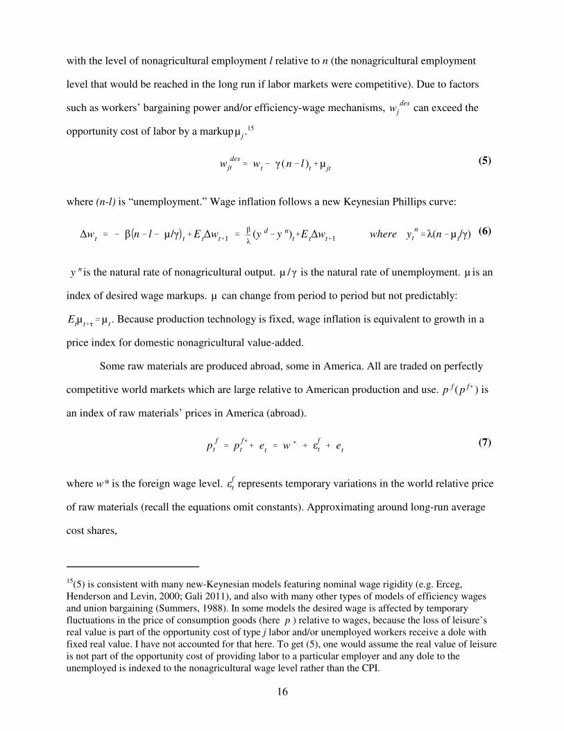
with the level of nonagricultural employment l relative to n (the nonagricultural employment

level that would be reached in the long run if labor markets were competitive). Due to factors

such as workers’ bargaining power and/or efficiency-wage mechanisms, can exceed thewdes

j

opportunity cost of labor by a markup .15 µj

where (n-l) is “unemployment.” Wage inflation follows a new Keynesian Phillips curve:

is the natural rate of nonagricultural output. is the natural rate of unemployment. is any n µ /γ µ

index of desired wage markups. can change from period to period but not predictably:µ

. Because production technology is fixed, wage inflation is equivalent to growth in aEtµ

t%τ'µ

t

price index for domestic nonagricultural value-added.

Some raw materials are produced abroad, some in America. All are traded on perfectly

competitive world markets which are large relative to American production and use. ( ) isp f p f(

an index of raw materials’ prices in America (abroad).

where w* is the foreign wage level. represents temporary variations in the world relative priceεf

t

of raw materials (recall the equations omit constants). Approximating around long-run average

cost shares,

16Over 1932-1938, the value of imports of crude materials and foods rose and fell with real activity (roseover the 1933-36 recovery, fell over the 1936-38 downturn) but on average was about equal to the valueof exports of crude materials and foods (Historical Statistics of the United States, Millenium Edition,series Ee 446-457).

17

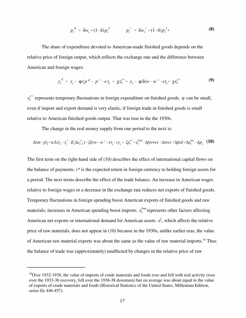
pd

t ' δwt% (1&δ)p

f

t p(

t ' δw(

t % (1&δ)pf

t ((8)

yd

t ' yt& n (p d& p (&e )

t% χε

y(

t ' yt& nδ(w&w (&e)

t% χε

y(

t(9)

∆(m&p)t'κ∆ (i

t& i

(

t &Et∆e

e

t%1)&ζδ (w&w (&e)t& ιy

t% ξε

y(

t %εbop

t &∆forres&∆tres%∆fed%∆εms

t &∆pt

(10)

The share of expenditure devoted to American-made finished goods depends on the

relative price of foreign output, which reflects the exchange rate and the difference between

American and foreign wages:

represents temporary fluctuations in foreign expenditure on finished goods. can be small,εy(

t φ

even if import and export demand is very elastic, if foreign trade in finished goods is small

relative to American finished-goods output. That was true in the the 1930s.

The change in the real money supply from one period to the next is:

The first term on the right-hand side of (10) describes the effect of international capital flows on

the balance of payments. i* is the expected return in foreign currency to holding foreign assets for

a period. The next terms describe the effect of the trade balance. An increase in American wages

relative to foreign wages or a decrease in the exchange rate reduces net exports of finished goods.

Temporary fluctuations in foreign spending boost American exports of finished goods and raw

materials; increases in American spending boost imports. represents other factors affectingεbop

t

American net exports or international demand for American assets. , which affects the relativeεf

price of raw materials, does not appear in (10) because in the 1930s, unlike earlier eras, the value

of American raw material exports was about the same as the value of raw material imports.16 Thus

the balance of trade was (approximately) unaffected by changes in the relative price of raw

18

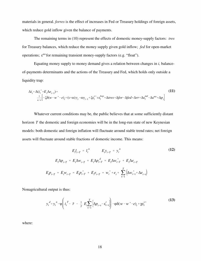
∆it'∆(i

(

t %Et∆e

t%1)%

1

κ%ν&ζδ(w&w (&e)

t% (ι%ω)y

t&ωy

t&1%ξε

y(

t Kεbop

t %∆tres%∆for&∆fed%∆rr%∆εmd

t &∆εms%∆pt

(11)

Etlt%T

' ln

t Ety

t%T' y

n

t

Et∆p

t%T' E

t∆w

t%T' E

t∆p

d

t%T ' Et∆w

(

t%T % Et∆e

t%T

Etp

t%T' E

tw

t%T' E

tp(

t%T % Ete

t%T' w

(

t %et% j

T

τ'1

∆w(

t%τ%∆et%τ

(12)

yd

t 'yn

t &ψ iT

t & r &1

TE

tjT

τ'1

∆pt%τ&ε

r

t%τ &φδ(w&w (&e)t%χε

y(

t

(13)

materials in general. forres is the effect of increases in Fed or Treasury holdings of foreign assets,

which reduce gold inflow given the balance of payments.

The remaining terms in (10) represent the effects of domestic money-supply factors: tres

for Treasury balances, which reduce the money supply given gold inflow; fed for open-market

operations; for remaining transient money-supply factors (e.g. “float”).εms

Equating money supply to money demand gives a relation between changes in i, balance-

of-payments determinants and the actions of the Treasury and Fed, which holds only outside a

liquidity trap:

Whatever current conditions may be, the public believes that at some sufficiently distant

horizon the domestic and foreign economies will be in the long-run state of new KeynesianT

models: both domestic and foreign inflation will fluctuate around stable trend rates; net foreign

assets will fluctuate around stable fractions of domestic income. This means:

Nonagricultural output is thus:

where:

19

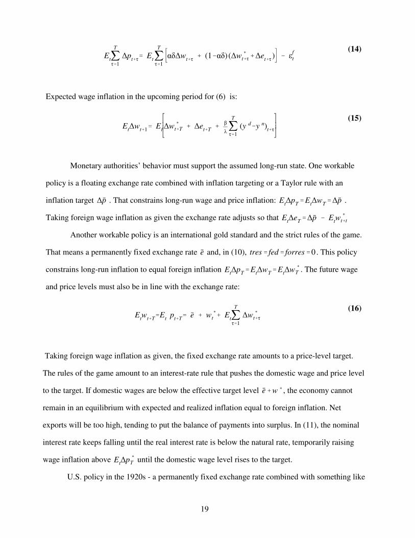
Etj

T

τ'1

∆pt%τ' E

tjT

τ'1

αδ∆wt%τ

% (1&αδ) (∆w(

t%τ%∆et%τ

) & εf

t

(14)

Et∆w

t%1' E

t∆w

(

t%T % ∆et%T

%β

λjT

τ'1

(y d&y n)t%τ

(15)

Etw

t%T'E

tp

t%T' e % w

(

t % Etj

T

τ'1

∆w(

t%τ

(16)

Expected wage inflation in the upcoming period for (6) is:

Monetary authorities’ behavior must support the assumed long-run state. One workable

policy is a floating exchange rate combined with inflation targeting or a Taylor rule with an

inflation target . That constrains long-run wage and price inflation: .∆p Et∆p

T'E

t∆w

T'∆p

Taking foreign wage inflation as given the exchange rate adjusts so that Et∆e

T'∆p & E

tw

(

t%t

Another workable policy is an international gold standard and the strict rules of the game.

That means a permanently fixed exchange rate and, in (10), . This policye tres' fed' forres'0

constrains long-run inflation to equal foreign inflation . The future wageEt∆p

T'E

t∆w

T'E

t∆w

(

T

and price levels must also be in line with the exchange rate:

Taking foreign wage inflation as given, the fixed exchange rate amounts to a price-level target.

The rules of the game amount to an interest-rate rule that pushes the domestic wage and price level

to the target. If domestic wages are below the effective target level , the economy cannote%w (

remain in an equilibrium with expected and realized inflation equal to foreign inflation. Net

exports will be too high, tending to put the balance of payments into surplus. In (11), the nominal

interest rate keeps falling until the real interest rate is below the natural rate, temporarily raising

wage inflation above until the domestic wage level rises to the target.Et∆p

(

T

U.S. policy in the 1920s - a permanently fixed exchange rate combined with something like

20

yd

t 'yn

t &ψ iT

t &1

T(E

tw

t%T&w

t)& r %ε

f

t &1

TE

tjT

τ'1

(1&αδ)∆w(

t%τ&εr

t%τ &φδ(w&w (&e)t%χε

y(

t

(17)

Etw

t%T&w

t'TE

t∆w

(

t%T %β

λE

tjT

τ'1

(y d&y n)t%τ

(18)

∆wt'

β

λ(y d&y n)

t%E

t∆w

(

t%T %β

λjT

τ'1

(y d&y n)t%τ

(19)

inflation targeting or a Taylor rule - was tenable in the short run because the domestic wage level

was less than , so the balance of payments was in surplus. In the long run, one possiblee%w (

outcome was for American authorities to stop accumulating gold and foreign assets, allow the

money supply to grow faster, interest rates to fall, output to rise above the natural rate and inflation

to occur. But another possible outcome was a decline in foreign wage inflation to lower . e%w (

Now consider a situation corresponding to early 1933: output far is below the natural rate;

the exchange rate is fixed by the dollar’s gold parity; the overnight rate is zero. Under the

conventional view of the liquidity trap, a zero overnight rate means i is zero, so that demand for

high-powered money is indeterminate. (I will return to this later.) The public expects the economy

will lift off from the zero bound by some future point in time. The horizon T is, by definition, well

past this point. What is the effect of a policy package like Roosevelt’s? For simplicity, I describe

the policy as an unexpected one-time devaluation, with no expectations of further devaluation. The

latter would only reenforce the effects I describe here.

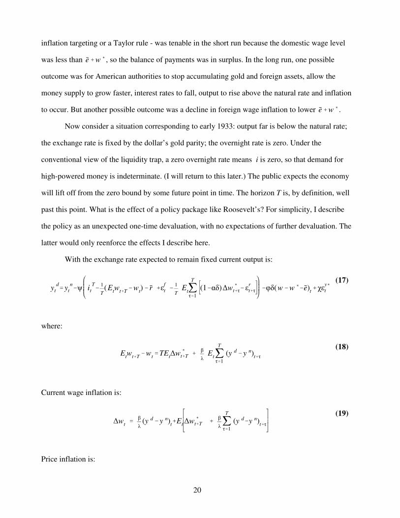
With the exchange rate expected to remain fixed current output is:

where:

Current wage inflation is:

Price inflation is:

21

∆pt' αδ∆w

t% (1&αδ) (∆w

(

t % ∆et) % (1&δ)∆ε

f

t

∆pd

t ' δ∆wt% (1&δ) (∆w

(

t % ∆εf

t % ∆et)

(20)

Devaluation causes an immediate increase in domestic price inflation simply by raising raw

materials’ prices. By reducing the relative price of domestic goods devaluation also tends to boost

net exports, with a small effect on domestic output and a potentially large effect on high-powered

money growth through unsterilized gold inflows. But with the short-term rate at the zero bound,

current money growth has no direct effect on interest rates.

The expected-inflation channel runs through the public’s expectations of the future path of

the output gap in (18). If the public believes monetary authorities will follow the rules of the game

in one way or another, devaluation means that, for some periods in the span between liftoff and T,

real activity must be higher than it would absent devaluation: otherwise wages cannot rise to match

the new exchange rate. For any given long-term yield in (17), that tends to decrease the long-i T

term real rate, boosting current output. (There may also be a decrease in due to expectations ofi T

lower nominal short-term rates in the post-trap future.) In (19), the increase in current output tends

to raise wage inflation in the ordinary way. But the key point is this: due to expected-inflation

mechanism there will be a further extraordinary increase in wage inflation through the second term

on the right-hand side, that is through expected future wage inflation.

Given the experience of the 1920s the public could have doubted that authorities would

actually allow future inflation to take place. Roosevelt’s pro-inflation statements, the presence of

inflation supporters in Congress and the absence of sterilization over 1934-36 could have made a

difference in this respect. By the same token, the public could have taken reserve-requirement

increases and gold sterilization over 1936-37 to indicate the Fed was likely to revert to its 1920s

policies after all. Thus, the expected-inflation channel might have tended to decrease output in

1936-37. If it did, it should also have caused an extraordinary decrease in wage inflation.

2.2) Evidence of the expected-inflation mechanism in the 1930s

17A great variety of evidence from the 1930s and other eras shows that banking crises have enormous realeffects (e.g. Bernanke, 1983; Richardson and Troost 2009; James, McAndrews and Weimanforthcoming). On 1937 see Meltzer (2003:521-22), Currie (1938).

18 Two studies attempt to infer inflation expectations in the 1929-32 downturn of the Great Depression

indirectly. Cechetti (1992) produces statistical forecasts based on information available at the time,specifically lagged inflation and nominal interest rates. Hamilton (1992) uses agricultural commodityfutures prices from the period. Their methods are obviously inappropriate for my purpose here. Cechettiforecasts future inflation from past inflation, and from nominal interest rates on the assumption that thereal interest rate is stationary. If the expected-inflation channel is effective, those conditions do not hold.Hamilton’s procedure assumes both rational expectations and a stable (stochastic) relationship betweencommodities prices and the price level. The relationship between commodities prices and the price levelwould be affected by changes in exchange rates and by the Roosevelt administration’s agriculturalprograms. (That was the point of the programs!)

19The only obvious difference between 2008-12 and 1933-34 is that, in the earlier era, the Wall Street

Journal’s analysis was relatively insightful.

22

Did devaluation and pro-inflation rhetoric over 1933-34, and monetary policy turns later in

the 1930s, really affect output through the expected-inflation channel? The cyclical upturn in April

1933 and downturn in 1937 are consistent with an expected-inflation mechanism, but there are

other obvious explanations of both events: in 1933, the resurrection of the banking system from

total breakdown; in 1937 a fiscal tightening among other things.17 I know of no surveys from the

1930s that could be taken to indicate long-term inflation expectations directly.18 I have examined

newspapers and magazines from the era, following Nelson (1991) who attempts to discern inflation

expectations over 1929-30 from an examination of the era’s business publications. Clearly, the

policies were of great public interest. While the Roosevelt administration was actively

manipulating the dollar’s gold price in late 1933, its daily value was front page news (Pearson,

1957, p. 5644). But I cannot find a dominant view of the policies’ effects. They were variously

described as impotent and as a cause of inevitable hyperinflation. Discussions of monetary policy

in the press were as contradictory as in our own post-2008 era.19

A distinctive sign of the expected-inflation channel is anomalous movements in inflation.

That is what I look for here. I estimate Phillips-curve relationships in data from the post-World

War II era. I apply the estimated postwar coefficients to the path of real activity after 1929 to

project a path for inflation over 1929-1940. I ask whether the actual path of inflation deviates from

23

the projected path in ways consistent with effects of the expected-inflation channel. Simple new

Keynesian models like that outlined above imply that the channel’s effects on inflation must be

coincident with effects on output and the public’s receipt of relevant news about policy, because

inflation and spending respond at once to changes in real interest rates and expected inflation. As

Svennson (2000) points out, this feature of new Keynesian models cannot be taken seriously. More

realistic models imply lags in the response of spending and inflation to shocks. Thus, I will look

for any kind of loose, perhaps delayed relation between inflation and policy turns.

As for Akerlof, Dickens and Perry (1996), my baseline Phillips curve is a simple regression

of inflation on current real activity and two past years of inflation. To avoid direct effects of

devaluation on product prices through raw-materials prices, I look at inflation in nonagricultural

wages. Price indexes for nonagricultural value-added from the National Income and Product

Accounts would also be appropriate, but for the 1930s NIPAs are available only at an annual

frequency. For my purposes, data must be higher frequency and comparable between the 1930s and

the postwar era - constructed in the same way with the same biasses. Monthly data on average

hourly earnings in manufacturing, the main nonagricultural sector, fit the bill. It would be useful to

compare 1930s inflation with projections from pre-1914 Phillips curves. But no 1930s wage series

are comparable with long runs of pre-1914 data.

A problem with applying postwar coefficients to project inflation in an earlier era is a well-

known historical shift in the empirical Phillips curve. Data that span years from the late 1960s

through the early 1990s fit the “accelerationist” Phillips curve: coefficients on lagged inflation are

positive, statistically significant and of a magnitude that indicates a nearly one-to-one relation

between recently-experienced inflation and current inflation. Data from the pre-1914 era and the

1920s fit the original Phillips curve: coefficients on lagged inflation are small and usually not

significantly different from zero at conventional levels (Gordon, 1990; Alogoskoufis and Smith,

1991; Allen, 1992; Hanes, 1993). I create 1930s projections from postwar coefficients in two ways.

In one I apply both the real-activity and lagged-inflation coefficients. In the other I apply the

20In the first application of the Phillips curve to American data, Samuelson and Solow (1960:188) foundthat "the years from 1933 to 1941 appear to be sui generis: money wages rose or failed to fall in the faceof massive unemployment" (p. 188). See also Friedman and Schwartz (1960: 498), Gordon (1983).

21The NIRA required employers to negotiate with employee representatives, but it was not clear that thismeant independent unions. Auto industry employers wanted NRA administrators to allow the industry toremain nonunion. They gave raises in June and July to demonstrate that unions were not needed to raiseindustry wages (Fine, p. 48-49 and p. 444 note 12).

24

postwar real-activity coefficient but set the coefficients on lagged inflation to zero. As it turns out,

there is little difference for my purposes between projections with lagged-inflation coefficients on

versus off. From 1929 through 1932 they follow about the same paths and fit actual wage inflation

very tightly. From 1933 on actual inflation deviates from both with about the same timing.

It is well known that data from 1933-1940 deviate from any formulation of the Phillips

curve.20 Akerlof, Dickens and Perry (1996) argue that these deviations were due to “downward

nominal wage rigidity” (a special constraint on nominal wage cuts). Blanchard and Summers

(1986) argue they may reflect “hysteresis” in the natural rate of unemployment as laid-off workers

lose membership in insider bargaining groups. I will not run the expected-inflation channel in a

horserace against these alternative theories. But there are other extraordinary influences on wages

in the 1930s, matters of fact, that must be accounted for.

The NIRA and unionization

The National Industrial Recovery Act (NIRA), passed in June 1933, applied to nearly all

nonagricultural employers. The NIRA affected wages directly through the employment provisions

of industry “codes,” which included industry-specific minimum wage rates. According to all

accounts adoption of minimum wages raised wages of all workers because employers generally

attempted to maintain pre-existing differentials. As soon as June 1933 auto manufacturers began to

give raises to "improve their bargaining power in code negotiations" (Fine 1963: 125).21 The first

industry code, in cotton textiles, came into effect in July 1933 and was estimated to raise industry

average wage rates substantially (Sachs, 1934: 147). At the end of July 1933 Roosevelt “invited”

nearly all nonagricultural employers in industries that had not yet adopted their own codes to sign

22The blanket code fixed minimum hourly wage rates, maximum weekly hours and minimum weeklyearnings, and required "equitable" maintenance of differentials above the minimums for higher-paidworkers (Sachs 1934, 131).

25

the “President’s Re-Employment Agreement,” known as the “blanket code.” Its provisions required

most employers to raise wages. It came into effect in August.22 Between August and December

1933 industries representing the bulk of employment adopted their own codes; by June 1934 all

industries had been codified (United States 1935: Chart 36). Industry codes created pay hikes

beyond those associated with the blanket code. They required more wage hikes and changes in

compensation policies such as premium pay for overtime (Schoefeld, 1935; Weinstein, 1980, 9;

17; 47).

In addition to (but interacting with) establishing the code process, the NIRA stated that

employees had a right to organize for collective bargaining. The enforcement agency established by

the NIRA, the National Recovery Administration (NRA), took months to work out what this meant

in specific regulations and create institutional structures to enforce them. But workers immediately

understood the NIRA to bar employers from replacing strikers or firing employees attempting to

organize a union. The number of workers involved in new strikes, plotted in Figure 6, increased

enormously from May to June 1933. It remained much higher through the rest of the 1930s than it

had been in the late 1920s.

The NIRA was declared unconstitutional in May 1935 but most of its pro-union elements

were re-established and strengthened by the Wagner Act (National Labor Relations Act) passed in

July 1935 (Mills and Brown 1950). In November 1936 "The overwhelming Roosevelt victory" in

the presidential election "led employers to expect aggressive organizing drives by trade

unions...wage rates were influenced by the large number of industrial disputes and by the efforts of

employers to forestall unions by making concessions" (Slichter 1938: 98-99). In April 1937 the

Supreme Court ruled the Wagner Act constitutional, and many companies that had refused to

bargain with elected unions despite the Wagner Act gave in (Fine, 1963: 415; Schatz, 1983: 70).

Estimates of union membership, which are annual (and imperfect), indicate enormous increases in

23In March 1934 auto manufacturers gave a general ten percent wage increase “with a view tostrengthening their position with the administration, their workers, and the public at a time when the A.F.of L. federal labor unions in their plants, for whose existence the N.I.R.A. was largely responsible, werethreateneing an industry-wide strike”; but at the time no union had signed up a majority of workers in anyauto firm, and neither the automakers nor the NRA had recognized any union as a bargaining agent forworkers (Fine, 1963:125,142). In March 1937 the nonunion Westinghouse Corporation raised wages inresponse to General Electric’s recognition of a union (Schatz 1983: 67). The Allis-Chambers Corporationdid not have an NLRB-certified union until 1938, but in April 1936 “The impact of increasing unionpressure on the company was obvious” and it granted substantial bonuses (Peterson 1976:322). MostInternational Harvester plants were not unionized until 1941, but the company gave a number ofcompany-wide wage hikes in 1935 and 1936 to discourage unionization (Ozanne, 1967: 148, 178, 179).

26

∆wt%1' E

t[∆w

t%T%

β

λjT

τ'0

(y d&y n)t%τ

] ' Et[∆w

t%T%

β

λjT

τ'0

(y d&λn)t%τ

] %β

λ γµ

t

(21)

∆wt%1' E

t∆w

t%T%

β

λ

1

1&ρ(y d&λn)

t%

β

λ γµ

t% z

t(22)

union density in 1937 and 1938, as shown in Figure 6. But it is important to keep in mind that

workers’ bargaining power increased even in establishments that were not formally unionized.

Many firms that remained nonunion through the late 1930s raised wages at times over 1934-1938

to forestall union threats.23

What my exercise means in terms of the new Keynesian Phillips curve

My exercise is easy to interpret in terms of the new Keynesian Phillips curve. From above,

Current wage inflation is determined by - expected wage inflation at the long horizon -Et∆w

t%T

and the expected value of the cumulative output gap over the span from the current period to that

horizon. Assuming as I did above that the average wage mark-up is variable but unpredictable, the

cumulative output gap can be broken into two components: the expected deviation from trend in

output and a factor reflecting variations in the average wage markup - a “supply shock.”

Suppose that in the absence of changes in the monetary regime the relation between current

output and wagesetters’ expectation of future output can be approximated by an AR(1) with

coefficient . For real GDP in the postwar era, a simple autoregressive univariate forecast like thisρ

is hard to beat (Faust and Wright, 2007). Then:

24In the postwar era, professional economic forecasters have reported long-run inflation expectations insurveys. From the late 1960s through the early 1990s reported long-run expected inflation varied fromyear to year and was positively correlated with recently experienced inflation. Estimates of long-termexpected inflation extracted from long-term interest rates have been unstable and strongly affected bynews about inflation and economic activity (Gurkaynak, Sack and Swanson, 2005). Erceg and Levin(2003) show that a New Keynesian DSGE model reproduces postwar price-inflation movements fairlywell assuming long-term inflation expectations responded to experienced macroeconomic conditionswith magnitudes calibrated to the survey data.They argue that expectations were rational but, especiallyover the 1980s, realized inflation did not reflected the ex ante distribution: wage- and price-settersaccounted for a possible but unrealized future in which monetary policy would accommodate high,persistent inflation. That is, there was a “peso problem.” I know of no survey data on inflationexpectations from the pre-1914 era, but the behavior of long-term interest rates in the pre-1914 eraindicates long-term price inflation expectations were stable, remarkably unresponsive to experiencedmacroeconomic events (Bordo and Dewald, 2001). Barsky and DeLong (1991) find evidence that thelong-term inflation expectations indicated by pre-1914 interest rates were perhaps too stable to berational expectations: they failed to respond to data on gold production, available at the time, whichturned out to predict realized inflation. But they also point out, like Erceg and Levin (2003) for thepostwar era, that one cannot judge the rationality of expectations on the basis of distributions of observedoutcomes. From a late-nineteenth century point of view, there were many possible relations between golddiscoveries and inflation; the “theory” that turned out to be correct ex post was just one of many ex ante

possibilities. Again, a peso problem.

27

represents the difference between the univariate forecast and wagesetters’ actual forecast forz

cumulative future output. When the expected-inflation channel is (decreasing) output, z is positive

(negative).

(22) is consistent with empirical Phillips curves from both the pre-1914 and postwar eras

assuming that in both eras the expected-inflation mechanism and changes in average markups were

unimportant. (22) generates the pre-1914 pattern if is uncorrelated with recent inflation.Et∆w

t%T

(22) generates the postwar pattern if, within the sample examined, is strongly correlatedEt∆w

t%T

with recent inflation. Much evidence confirms this is a good description of the behavior of

expected inflation in the two eras.24 For the 1930s, one might guess expectations followed the pre-

1914 pattern until U.S. adherence to its the gold exchange rate came into question. That was, at the

earliest, September 1931 when Britain devalued: at that time some financial-market participants

began to bet the U.S. would too (Friedman and Schwartz, 1963, p. 316). The long-term inflation

expectation might have been similarly stable after 1934, if the public believed the 1934 devaluation

was a one-time thing. That would mean the baseline empirical Phillips curve for the 1930s, absent

extraordinary factors, should follow the pre-1914 pattern - no positive coefficients on lagged

25 They are from surveys carried out by the National Industrial Conference Board beginning in 1920, andby the Bureau of Labor Statistics beginning in 1934, as described by Dighe (1997).

28

inflation.

At the same time, there are problems with simply turning off positive postwar lagged-

inflation coefficients to generate a projection for periods when was stable. A postwarEt∆w

t%T

coefficient on real activity has positive bias as an estimate of in (22) if real activity was(β

λ

1

1&ρ)

positively correlated with changes in . That is likely: long-horizon inflation expectationsEt∆w

t%T

reported in surveys declined in the recessions of 1973, 1981 and 1991. On the other hand,

measurement error in indicators of real activity creates the opposite bias, toward zero. Both these

worries are minor next to another shaky assumption for the exercise: that the baseline relation

between current real activity and forecasts of future real activity, absent the expected-inflation

channel, was the same in the earlier eras as in the postwar era. In the end, the proof of the

projections is their fit to actual wage inflation over the span between 1929 and March 1933, prior

to the possible operation of the expected-inflation channel. As it turns out, the fit is very good.

Deviations from projections may reflect z, the expected-inflation channel. The problem is

that they may also reflect changes in . All of my real-activity measures, including theµ

unemployment rate series, are essentially deviations of output or employment from fixed trends.

They do not account for changes in in any way. Features of the NIRA and later New Dealµ

legislation that protected union organizers and hindered replacement of strikers increased . Otherµ

features of the NIRA simply broke the relationship described by (22). The NIRA’s minimum

wages cannot be described as increases in because they were nominal. Employers negotiatingµ

with the NRA knew that NRA administrators wanted to prevent nominal wage cuts, above all.

Data

1930s data on average hourly earnings in manufacturing by industry are comparable with

postwar data.25 Hanes (1996) matched 1930s industries to industries in postwar data and applied

fixed industry weights to construct a manufacturing AHE series that is consistent from the 1920s

26Estimates apparently at a higher frequency such as Balke and Gordon’s (1986) are actuallyinterpolations between annual estimates based mainly on IP.

27Postwar unemployment data are based on household surveys that allow people to classify themselves asin or out of the labor force (on BLS definitions). For years before 1940 no such surveys are available.Unemployment must be estimated as the difference between employment estimates and the long-termtrend "usual labor force" (indicated by population censuses). In one sector, agriculture, there is noreliable way to estimate short-term variations in employment absent household survey data since so muchfarm labor is family labor. There is no consensus on whether the large numbers of Federal relief workersin the 1930s should be classified as employed or unemployed (see Darby, 1976 versus Lebergott, 1964).Weir's estimate of the private nonfarm unemployment rate sidesteps these problems. Its denominator isthe "usual labor force," estimated the same way, for postwar years up to 1990 and earlier years. Itexcludes agriculture, government and relief workers from both the employment and labor force figures.Within the 1920-30s its underlying estimates for private nonagricultural employment are not significantlydifferent from those underlying the alternative unemployment series of Lebergott (1964) and Romer(1986).

28It is tricky to define trends for the Great Depression era. It is clearly inappropriate to use a Hodrick-Prescott trend with conventional parameters or a loglinear trend estimated within the interwar era alone.Either would imply output was close to trend or even above trend in the mid-1930s, which is inconsistentwith all unemployment estimates. I follow Romer (1989) and Balke and Gordon (1989) and define trendsby loglinear interpolation between benchmark "normal" years. They use 1924, 1947, 1955, 1962, 1972,and 1981. I add two more benchmarks: 1941 and 1990. Using these benchmarks, output was far below

29

through 1990. Industry-level AHE reflect many things other than wage rates (the distribution of

workers across a given firm’s wage structure, the distribution of employment between high- and

low-wage firms, the fraction of hours paid at premium rates). To make sure key movements in

AHE actually reflect changes in wage rates I will check them against a wage index from the 1930s

(which is unfortunately not comparable with any postwar series).

To project 1930s wage inflation at a monthly frequency my real-activity indicator is the

Federal Reserve Board Index of Industrial Production. For the 1930s estimates of real GDP and

unemployment rates are available only at an annual frequency.26 Mainly as a check on monthly

projections I make 1930s projections of annual inflation using NIPA real gross output of nonfarm

private business, and David Weir’s (1992) series for the "private nonfarm unemployment rate."

Weir constructs his series in the same way across the 1930s and the postwar era up to 1990. Unlike

postwar BLS unemployment series, it does not account for short-term fluctuations in the labor

force - it is essentially deviation from a long-term trend in employment.27 Figure 4 plots Weir’s

series. For IP and real GDP, "real activity" is the deviation of the log from a long-term trend.28

"potential" throughout the 1930s. Cole and Ohanian (1999, footnote 5) define trends by estimating one

loglinear trend spanning both 1919-1929 and postwar years, and assuming 1929 was on trend, so that the

trend level for 1930 is the 1929 level plus the trend growth rate. I tried that too but it made littledifference to my conclusions so I present only the results from the benchmark-year trends.

29 Rockoff (1984) gives chronologies of the Korean War and Nixon controls. Korean War controls were

lifted in February 1953, plausibly affecting the rate of wage inflation from 1953 to 1954. With two years'lagged inflation in my specifications, I begin with 1956. The Nixon controls held in one form or another

from August 1971 through April 1974 (affecting inflation from 1974 to 1975). For monthly data the

sample runs from March 1955 through July 1971 and from May 1976 through December 1990.

30

Inflation projections

Hanes and James (2012) give details on the postwar Phillips curve regressions and the

estimated coefficients. To avoid years affected by wage and price controls, the postwar samples

run 1956-1971/ 1977-1990.29 Within the postwar era the regression coefficients give more or less

unbiassed projections of disinflations in cyclical downturns. For monthly-frequency regressions the

dependent variable is the change in the log of the AHE series from the same month in the prior

year. Month-to-month changes would be sensitive to precise definition of seasonals. There is good

reason to believe NRA code adoption affected AHE seasonals strongly. (Many codes introduced

worksharing, stabilization of hours and premium pay, among other things).

Going back to the 1930s I project wage inflation starting with January 1929. The

projections using lagged inflation jump off from actual wage inflation in 1927 and 1928. From

1930 on the lagged inflation rates entering projections are lagged projections.

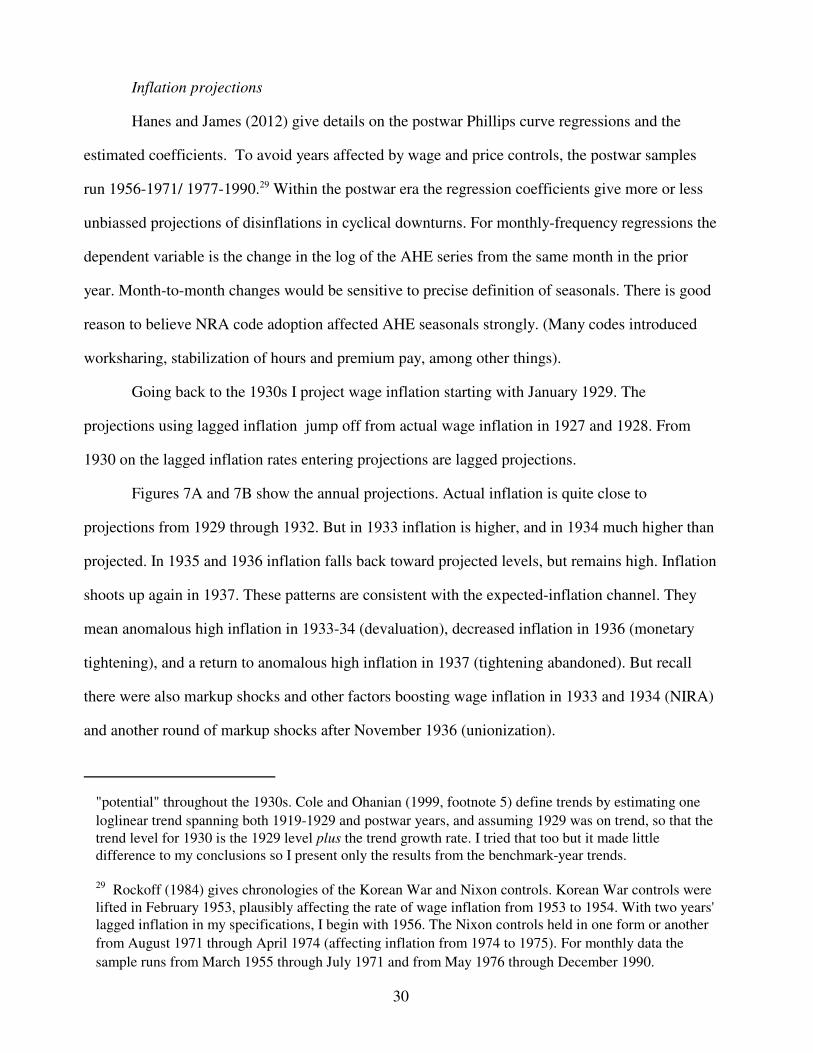
Figures 7A and 7B show the annual projections. Actual inflation is quite close to

projections from 1929 through 1932. But in 1933 inflation is higher, and in 1934 much higher than

projected. In 1935 and 1936 inflation falls back toward projected levels, but remains high. Inflation

shoots up again in 1937. These patterns are consistent with the expected-inflation channel. They

mean anomalous high inflation in 1933-34 (devaluation), decreased inflation in 1936 (monetary

tightening), and a return to anomalous high inflation in 1937 (tightening abandoned). But recall

there were also markup shocks and other factors boosting wage inflation in 1933 and 1934 (NIRA)

and another round of markup shocks after November 1936 (unionization).

30The timing of NRA effects has been misunderstood by authors of some existing studies of 1930sinflation. McCloskey and Zecher (1984, 141) suppose that they were coincident with code adoption; thatis certainly incorrect.

31

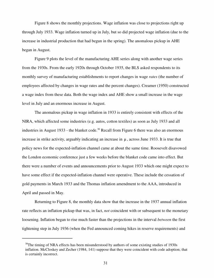
Figure 8 shows the monthly projections. Wage inflation was close to projections right up

through July 1933. Wage inflation turned up in July, but so did projected wage inflation (due to the

increase in industrial production that had begun in the spring). The anomalous pickup in AHE

began in August.

Figure 9 plots the level of the manufacturing AHE series along with another wage series

from the 1930s. From the early 1920s through October 1935, the BLS asked respondents to its

monthly survey of manufacturing establishments to report changes in wage rates (the number of

employees affected by changes in wage rates and the percent changes). Creamer (1950) constructed

a wage index from these data. Both the wage index and AHE show a small increase in the wage

level in July and an enormous increase in August.

The anomalous pickup in wage inflation in 1933 is entirely consistent with effects of the

NIRA, which affected some industries (e.g. autos, cotton textiles) as soon as July 1933 and all

industries in August 1933 - the blanket code.30 Recall from Figure 6 there was also an enormous

increase in strike activity, arguably indicating an increase in , across June 1933. It is true thatµ

policy news for the expected-inflation channel came at about the same time. Roosevelt disavowed

the London economic conference just a few weeks before the blanket code came into effect. But

there were a number of events and announcements prior to August 1933 which one might expect to

have some effect if the expected-inflation channel were operative. These include the cessation of

gold payments in March 1933 and the Thomas inflation amendment to the AAA, introduced in

April and passed in May.

Returning to Figure 8, the monthly data show that the increase in the 1937 annual inflation

rate reflects an inflation pickup that was, in fact, not coincident with or subsequent to the monetary

loosening. Inflation began to rise much faster than the projections in the interval between the first

tightening step in July 1936 (when the Fed announced coming hikes in reserve requirements) and

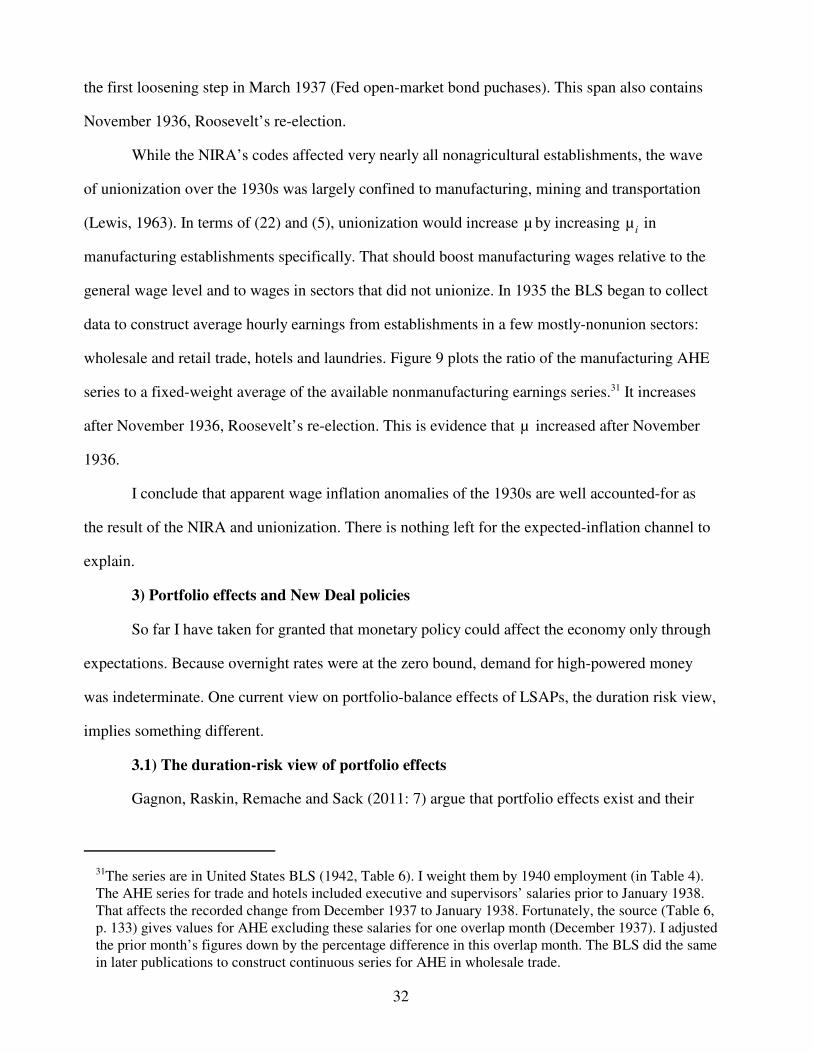
31The series are in United States BLS (1942, Table 6). I weight them by 1940 employment (in Table 4).The AHE series for trade and hotels included executive and supervisors’ salaries prior to January 1938.That affects the recorded change from December 1937 to January 1938. Fortunately, the source (Table 6,p. 133) gives values for AHE excluding these salaries for one overlap month (December 1937). I adjustedthe prior month’s figures down by the percentage difference in this overlap month. The BLS did the samein later publications to construct continuous series for AHE in wholesale trade.

32

the first loosening step in March 1937 (Fed open-market bond puchases). This span also contains

November 1936, Roosevelt’s re-election.

While the NIRA’s codes affected very nearly all nonagricultural establishments, the wave

of unionization over the 1930s was largely confined to manufacturing, mining and transportation

(Lewis, 1963). In terms of (22) and (5), unionization would increase by increasing inµ µi

manufacturing establishments specifically. That should boost manufacturing wages relative to the

general wage level and to wages in sectors that did not unionize. In 1935 the BLS began to collect

data to construct average hourly earnings from establishments in a few mostly-nonunion sectors:

wholesale and retail trade, hotels and laundries. Figure 9 plots the ratio of the manufacturing AHE

series to a fixed-weight average of the available nonmanufacturing earnings series.31 It increases

after November 1936, Roosevelt’s re-election. This is evidence that increased after Novemberµ

1936.

I conclude that apparent wage inflation anomalies of the 1930s are well accounted-for as

the result of the NIRA and unionization. There is nothing left for the expected-inflation channel to

explain.

3) Portfolio effects and New Deal policies

So far I have taken for granted that monetary policy could affect the economy only through

expectations. Because overnight rates were at the zero bound, demand for high-powered money

was indeterminate. One current view on portfolio-balance effects of LSAPs, the duration risk view,

implies something different.

3.1) The duration-risk view of portfolio effects

Gagnon, Raskin, Remache and Sack (2011: 7) argue that portfolio effects exist and their

33

fulcrum is “the reluctance of investors to bear the interest rate risk associated with holding an asset

that has a long duration.” In an LSAP, a central bank removes long-term bonds from private-sector

portfolios and replaces them with short-term bonds, or with reserves which are “zero-duration”

assets free of interest rate risk. “With less duration risk to hold in the aggregate, the market should

require a lower premium to hold that risk. This effect may arise because those investors most

willing to bear the risk are the ones left holding it. Or, even if investors do not differ greatly in their

attitudes toward duration risk, they may require lower compensation for holding duration risk when

they have smaller amounts of it in their portfolios.”

The duration-risk view of portfolio effects implies LSAPs are simple and effective. It does

not matter which long-term bonds the Fed buys: Treasuries will do. Because LSAPs compress term

premiums, they “should not only reduce longer-term yields on the assets being purchased but

should also spill over into the yields of other assets...Many private borrowers would find their

longer-term borrowing costs lower than they otherwise would be, and the value of long-term assets

held by households and firms, and thus aggregate wealth, would be higher” (2011: 8). It does not

matter much whether the Fed pays for LSAPs by selling very short-term bonds or by creating

reserves (as noted by Hamilton and Wu, 2012) . An operation that did not change private-sector

bondholdings at all but simply increased reserve supply - a “helicopter drop” of high-powered

money - would also work, because it would decrease the private sector’s relative holdings of assets

subject to interest-rate risk. Term premiums would have to fall to make banks willing to hold more

zero-duration assets.

The duration-risk view is not generally accepted, even among those who believe in

portfolio-balance effects. Krishnamurthy and Vissing-Jorgensen (2011) argue that the spread

between a bond’s yield and expected overnight rates depends on the relative supply of bonds of

that particular maturity and similar risk of default or prepayment (a possibility for mortgage-

derived securities). This “market segmentation version of the portfolio balance channel” (Bauer

and Rudebusch, 2012:6) - D’Amico et. al. (2012) call it the “scarcity” or “local-supply” effect -

implies LSAPs may fail to spur aggregate demand even if they affect some long-term bond yields,

34

because their effects are largely confined to the specific type of security being purchased: LSAPs in

Treasuries reduce only Treasury yields, not private-sector borrowing costs (Krishnamurthy and

Vissing-Jorgensen 2011: 285; Woodford, 2012: 65, 81).

3.2) Duration risk and money demand at the zero bound

Looked at from another angle, the duration-risk view implies demand for high-powered

money is not indeterminate when the overnight rate is zero. It is instead a function of expected

short-term returns to holding long-term liquid assets, as investors trade off expected return against

duration risk. From the 1930s through the 1950s, Keynesian literature analysed money demand in

these terms. Keynes (1936: 202) described the foregone interest earnings on money holdings as "a

sort of insurance premium to offset the risk of loss on capital account," referring specifically to the

risk that interest rates might rise above a current abnormally low level. Samuelson (1942: 594

footnote 3) observed "It is more and more being realized that reserves do not perform the function

of till money. Rather they are felt to be necessary for the maximization of income over time in a

world where uncertainty dictates a diversification of portfolios." Tobin (1958) showed that

uncertainty about future bond prices together with “risk-avoiding behavior,” implies "an inverse

relationship between the demand for cash and the rate of interest” (:85). Viewing money demand

as determined by interest rates in general, Keynes described the liquidity trap in terms of long-term

rates. He admitted that open-market operations in bills were useless if bill rates had been driven to

zero, for in that case bills were equivalent to money, but there was still a well-determined demand

for money broadly defined as cash plus bills (Hicks 1982: 263). Thus, Keynes argued, a central

bank could drive down long-term rates by purchasing longer-term bonds (Keynes 1930: 371; 1936:

207).

To see the peculiar relation between duration risk and money demand at the zero bound,

suppose financial-market participants are certain the overnight rate will remain zero for an interval

of time, but beyond that interval the overnight rate may rise. (Beyond a further horizon referred to

as T above it is certain that the overnight rate will be above zero.) Bonds that pay off beyond the

horizon of possible lift-off from the zero bound are subject to duration risk. Short-term safe bills

35

EtP

t%1B

t% M

t&

q

2

Var(At%1

)

At

s.t. At' M

t% P

tB

t

(23)

md

t . at&

1

q

1

σP/E

tP

t%1

2 it

(1%it)2

Mit/Mm

d

t . & q σP/E

tP

t%12

(24)

that pay off within that horizon are equivalent to high-powered money (ignoring transactions costs,

taxes and so on). Bills and high-powered money together constitute a homogenous asset class I

refer to simply as “money.” Following Vayanos and Vila (2009), suppose that risk-averse

“arbitrageurs” interact with “preferred habitat” investors who have net demands for assets only at

specific maturities. Money has a preferred-habitat clientele of its own (for example households

without access to financial instruments whose money demand depends only on income and

spending). Arbitrageurs hold money and an optimal portfolio of liquid bonds. (Relative yields and

weights for bonds within the portfolio depend on interaction between arbitrageurs and preferred-

habitat investors as in Vayanos and Vila.) is the current unit price of this bond portfolio.Pt

Arbitrageurs have an expected value for P in the upcoming period and a variance for theEtP

t%1σ

2P

possible surprise reflecting duration risk on safe bonds and default probabilities for(Pt%1&E

tP

t%1)

riskier ones. The expected return to holding bonds one period is . Taking currentit'E

tP

t%1/P

t&1

assets as given an arbitrageur chooses a money balance and units of the bond portfolio toAt

Mt

Bt

carry into the upcoming period, acting to maximize:

where q is a risk-aversion coefficient. An arbitrageur trades off the expected value of next period’s

assets against variance scaled to assets. For realistic values of the resulting demand for money isi

in logs approximately:

Money demand is negatively related to the expected return to holding bonds one period. The slope

of the money-demand curve increases with arbitrageurs’ risk aversion and with the degree of

uncertainty about future bond prices.

In the 1930s, a prominent set of arbitrageurs holding money and liquid bonds was banks.

32Hanes (2006) derives an expression like (24) for a deposit-taking bank whose risk-aversion reflects acost of falling below a capital requirement, and compares this peculiar type of reserve demand at the zerobound with reserve demand in ordinary circumstances.

33Conventional “money-demand” functions specifying negative relations between bill rates andaggregates of cash and deposits held by nonbanks appear to hold perfectly well in the 1930s (Meltzer1963, p. 242; Gandolfi and Lothian 1976, p. 50).

36

Contemporary discussions of banking imply banks paid close attention to duration risk (Ayers

1937; Bradford 1941, p. 446-447; Meltzer 2003: 507) and actively managed the margin between

cash and bonds, even though reserves were far in excess of regulatory requirements (for example

Federal Reserve Board 1938, p. 7; Bradford 1941, p. 447). (24) implies banks’ demand for money

broadly defined - reserve balances, vault cash and safe bills - was negatively related to the expected

short-term return on liquid bonds, taking the volume of bank assets as given.32 For nonbank

arbitrageurs, the role of money in (24) might be played by demand deposits (which paid no interest

in the 1930s). That might create a further relation between expected bond returns and banks’

money demand through an effect of on bank assets: an increase in would drain deposits.33i i

Thus, the duration-risk view implies money demand was not indeterminate in the 1930s.

Exogenous shocks to high-powered money supply should have affected expected bond returns,

unless they were offset by changes in the supply of Treasury bills.

3.3) High-powered money supply shocks in the 1930s

A number of recent studies have analyzed financial and macroeconomic effects of post-

1933 monetary policies (Hanes, 2006; Calomiris, Mason and Wheelock, 2011; Irwin,

forthcoming), but not with reference to post-2008 debates about LSAP’s. Bernanke, Reinhart and

Sack (2004: 18) observe that the effect of unsterilized specie purchases from 1934 on “is

reasonably characterized as a successful application of quantitative easing,” but do not look into

the issue.

The Fed and Treasury engaged in some deliberate LSAPs in the 1930s. As tests of portfolio

effects these are, like post-2008 LSAPs or Operation Twist, complicated by the possibility of

effects through the signalling channel. In 1937 the Fed and Treasury bought Treasury bonds on

37

several occasions with the expressed intent of “monetary ease” or to counteract potential financial

effects of reserve-requirement hikes (Blum, 1959: 369-75; 378; Gordon and Westcott 1937: 107;

Crum, Gordon and Westcott 1938: 49). Over 1938-39, the Fed and Treasury attempted to “smooth”

Treasury yields by selling (buying) bonds against increases (decreases) in prices (Meltzer 2003 pp.

506-33, 546-49). These operations were presumably responses to observed or predicted changes in

yields due to other causes.

I focus on the period from late April 1934 through early July 1936. Within this period the

Fed did not engage in open-market operations except to replace maturing securities in its portfolio.

The Treasury did not engage in active foreign-exchange operations except for some days in January

1935 when the Treasury actively bought gold to fight an appreciation of the dollar (Blum 1959:

129). Growth in high-powered money was due to passive Treasury purchases of specie from

foreign sellers or domestic mining. The Treasury purchased domestic specie at a fairly steady rate

(judging from the available data, which are monthly [Federal Reserve Board 1943 table 156]) but

purchases of foreign gold varied due at least partly to factors unrelated to American conditions.

One important fluctuating factor was capital flight to the U.S. due to foreign political events such

as the rise of Hitler (Federal Reserve Board, 1936a: 8-11; 1936b: 311-312; Friedman and Schwartz

1963:544; Romer 1992:773).

Short-lived but substantial effects on the high-powered money supply also occurred

because of Treasury cash-flow management practices. Until a gold certificate was created,

deposited at the Fed and spent a gold purchase could be covered out of the Treasury’s accounts at

commercial banks. Meanwhile the value of purchased specie appeared in the Treasury’s books as

an increment to its Federal Reserve accounts or Treasury cash (Federal Reserve Board 1943, p.

365). In effect, the gold purchase was temporarily sterilized. The balance of tax payments,

spending, debt sales and repayments shifted funds between the Treasury’s accounts in commercial

banks and its accounts in the Federal Reserve system. The latter are not part of the high-powered

money supply. In sum, the short-run effect of specie purchases and Treasury payments on high-

powered money supply was equal to the change in the value of the Treasury’s specie stock less the

38

change in Treasury balances - the sum of Treasury cash and Treasury Fed accounts (Friedman and

Schwartz 1963: 506-508). Nowadays, the Fed attempts to counteract the effects of these factors on

reserve supply with open-market operations (Hamilton, 1997). It did not do so in the 1930s.

Importantly, there is no reason to believe that within this period week-to-week variations in

gold purchases or Treasury balances had any effect through a signalling channel. Figures on the

monetary gold stock and Treasury balances as of Wednesday were available to the public on Friday

morning (in the Fed release then called the FR 283, now the H.4.1). But these figures had no

implications for future monetary policy. They implied nothing about policymakers’ preferences or

private information. At the time no one claimed that they did (as far as I know).

Figure 5 shows short-term fluctuations in money supply due to interactions between gold

purchases and Treasury balances. They were accommodated by fluctuations in banks’ reserve

accounts rather than outstanding currency. Scaled to the economy, these fluctuations in reserve

supply were very large. Within April 1934-July 1936, week-to-week growth in nonborrowed

reserves ranged between a minimum of less than zero to a maximum of half a percent of 1934

GDP. The total of all Operation Twist operations of 1961 was about 1.7 percent of GDP; the total

of all the Fed’s second post-2008 LSAP operations (“QE2") was about 4 percent of GDP

(Swanson, 2011: 156).

Table 1 shows regression results that indicate the relation between gold purchases, Treasury

balances and money within 1934-36. In the 1930s the reserve-requirement maintenance period was

one week long, so Federal Reserve data are weekly. The first two columns show that gold

purchases and Treasury balances largely determined week-to-week changes in the high-powered

money supply, whether the latter is defined as cash plus nonborrowed reserves as for (1) or cash

plus total reserves as for (2). Column (3) shows the relation between these factors and “money”

broadly defined as the sum of high-powered money and outstanding Treasury bills (plus Treasury

certificates, another form of short-term Treasury debt sold for some of this period). Fed data on

outstanding Treasury bills in the 1930s are only for the final week in each month, but they give no

sign Treasury bill issuance counteracted fluctuations in the high-powered money supply. Money

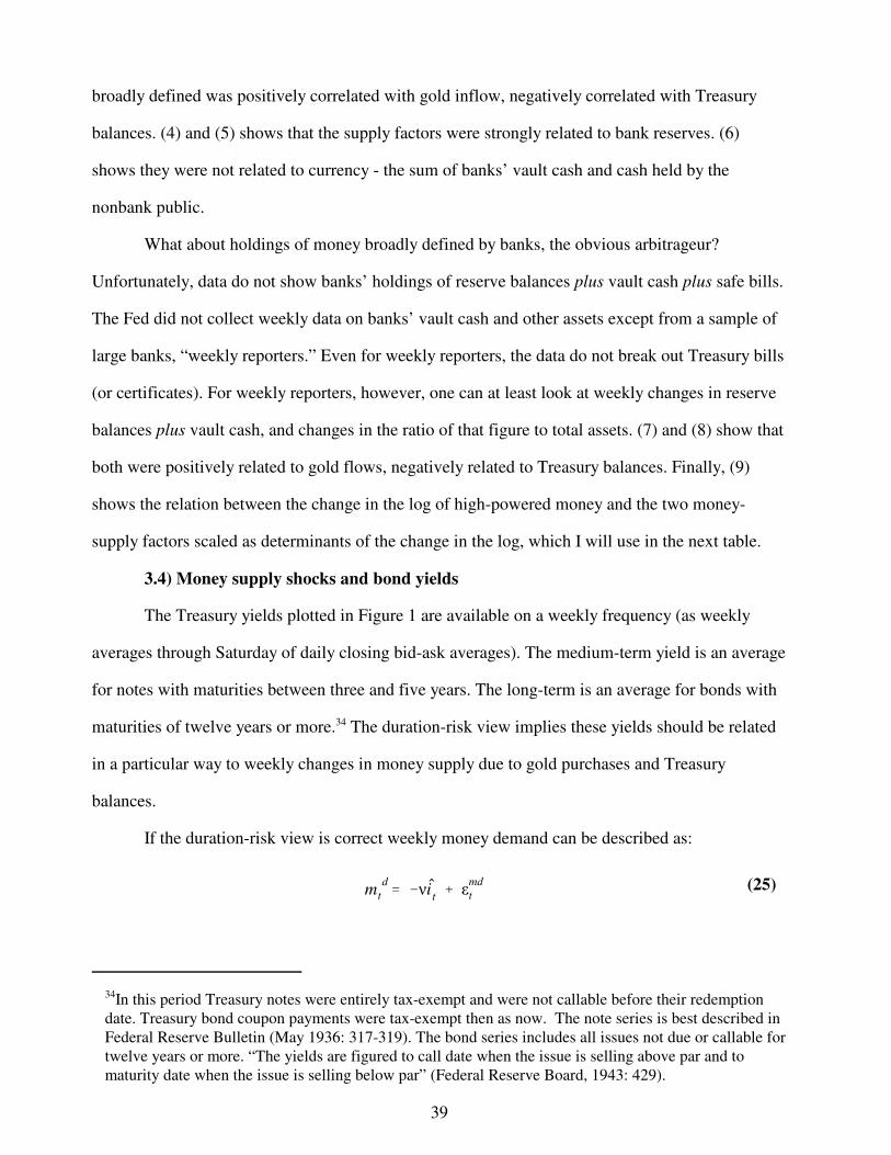
34In this period Treasury notes were entirely tax-exempt and were not callable before their redemptiondate. Treasury bond coupon payments were tax-exempt then as now. The note series is best described inFederal Reserve Bulletin (May 1936: 317-319). The bond series includes all issues not due or callable fortwelve years or more. “The yields are figured to call date when the issue is selling above par and tomaturity date when the issue is selling below par” (Federal Reserve Board, 1943: 429).

39

md

t ' &νit% ε

md

t(25)

broadly defined was positively correlated with gold inflow, negatively correlated with Treasury

balances. (4) and (5) shows that the supply factors were strongly related to bank reserves. (6)

shows they were not related to currency - the sum of banks’ vault cash and cash held by the

nonbank public.

What about holdings of money broadly defined by banks, the obvious arbitrageur?

Unfortunately, data do not show banks’ holdings of reserve balances plus vault cash plus safe bills.

The Fed did not collect weekly data on banks’ vault cash and other assets except from a sample of

large banks, “weekly reporters.” Even for weekly reporters, the data do not break out Treasury bills

(or certificates). For weekly reporters, however, one can at least look at weekly changes in reserve

balances plus vault cash, and changes in the ratio of that figure to total assets. (7) and (8) show that

both were positively related to gold flows, negatively related to Treasury balances. Finally, (9)

shows the relation between the change in the log of high-powered money and the two money-

supply factors scaled as determinants of the change in the log, which I will use in the next table.

3.4) Money supply shocks and bond yields

The Treasury yields plotted in Figure 1 are available on a weekly frequency (as weekly

averages through Saturday of daily closing bid-ask averages). The medium-term yield is an average

for notes with maturities between three and five years. The long-term is an average for bonds with

maturities of twelve years or more.34 The duration-risk view implies these yields should be related

in a particular way to weekly changes in money supply due to gold purchases and Treasury

balances.

If the duration-risk view is correct weekly money demand can be described as:

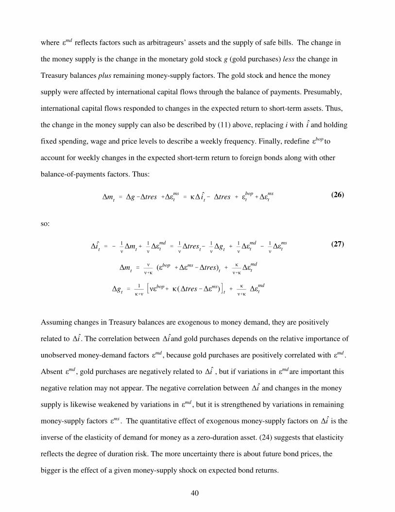
40

∆mt' ∆g&∆tres %∆ε

ms

t ' κ∆ it& ∆tres % ε

bop

t %∆εms

t(26)

∆it' &

1

ν∆m

t%

1

ν∆ε

md

t '1

ν∆tres

t&

1

ν∆g

t%

1

ν∆ε

md

t &1

ν∆ε

ms

t

∆mt'

ν

ν%κ(εbop %∆εms&∆tres)

t%

κ

ν%κ∆ε

md

t

∆gt'

1

κ%ννεbop% κ (∆tres&∆εms)

t%

κ

ν%κ∆ε

md

t

(27)

where reflects factors such as arbitrageurs’ assets and the supply of safe bills. The change inεmd

the money supply is the change in the monetary gold stock g (gold purchases) less the change in

Treasury balances plus remaining money-supply factors. The gold stock and hence the money

supply were affected by international capital flows through the balance of payments. Presumably,

international capital flows responded to changes in the expected return to short-term assets. Thus,

the change in the money supply can also be described by (11) above, replacing i with and holdingi

fixed spending, wage and price levels to describe a weekly frequency. Finally, redefine toεbop

account for weekly changes in the expected short-term return to foreign bonds along with other

balance-of-payments factors. Thus:

so:

Assuming changes in Treasury balances are exogenous to money demand, they are positively

related to . The correlation between and gold purchases depends on the relative importance of∆i ∆i

unobserved money-demand factors , because gold purchases are positively correlated with .εmd εmd

Absent , gold purchases are negatively related to , but if variations in are important thisεmd ∆i εmd

negative relation may not appear. The negative correlation between and changes in the money∆i

supply is likewise weakened by variations in , but it is strengthened by variations in remainingεmd

money-supply factors . The quantitative effect of exogenous money-supply factors on is theεms ∆i

inverse of the elasticity of demand for money as a zero-duration asset. (24) suggests that elasticity

reflects the degree of duration risk. The more uncertainty there is about future bond prices, the

bigger is the effect of a given money-supply shock on expected bond returns.

41

What do these relationships imply for Treasury yields, assuming Treasury balances and

gold purchases had no direct effect on expectations of future interest rates? Holding fixed

expectations of future bond prices, a decrease in the expected return to holding bonds for a short

period means an increase in today’s bond price. The effect on today’s yield to maturity is bigger for

shorter-term bonds. Thus, effects of money-supply factors should be stronger for bonds of shorter

maturity (but not so short that their yields are scraping the zero floor). Regressing changes in

medium-term yields on changes in the high-powered money supply or on the portion of money-

supply changes due to gold purchases and Treasury balances, the coefficient should be negative.

With gold purchases and Treasury balances separately on the RHS, the coefficient on Treasury

balances should be positive; the coefficient on gold purchases may or may not be negative

depending on the importance of money-demand shocks. Longer-term yields should give

coefficients of smaller magnitude.

Table 2 shows results of such regressions. I include quadratic time-trend terms on the

right-hand side but excluding these made no difference. The patterns are as predicted. The first

columns are for medium-term Treasuries. In (1) I use two-stage least squares with gold purchases

and Treasury balances as instruments for the change in the money supply. For (2) the sample

excludes the weeks in January 1935 when the Treasury was purchasing gold actively. For (3) the

RHS variable was just the money-supply change in OLS. Always, the coefficient on the money-

supply change is negative and significantly different from zero at the one percent level. For (4) I

include gold purchases along with the change in the money supply. This has little effect on the

money-supply coefficient, and the coefficient on gold purchases is not significantly different from

zero: clearly, the variable related to bond yields was the money supply not foreign purchases of

American assets as the latter variable would be more closely correlated with gold purchases. For

(5) gold purchases and Treasury balances are entered separately on the RHS. The coefficient on

Treasury balances is positive and significant at the one percent level; the coefficient on gold

purchases is negative but significant only at the ten percent level. The next columns are for long-

term Treasury bonds. Coefficients have the same sign as those for medium-term notes, but their

42

magnitudes are smaller so they are not significantly different from zero.

4) Conclusion

Roosevelt really did try Svennsson’s Foolproof Way out of a liquidity trap. Especially when

viewed in the context of gold-standard experience, his devaluation and pro-inflation jawboning

over 1933-34 could have had the same effect as adoption of a price-level target. But if you want

evidence that the expected-inflation option can work you must look elsewhere. Inflation anomalies

in the 1930s U.S. are easily explained by the NIRA and unionization. Of course, one could argue

these massive disturbances to wage inflation just obscured effects of the expected-inflation

channel. And if the expected-inflation channel did fail, it could have failed for two very different

reasons: because wagesetters’ expectations were insufficiently forward-looking, or because it was

rational to expect a future return to 1920s-style sterilization.

With respect to LSAPs, American experience from the 1930s gives much clearer evidence:

when overnight rates are at the zero bound, central banks can still influence long-term rates

through portfolio effects. Over 1934-36 weekly fluctuations in the high-powered money supply

were correlated with changes in medium- and long-term Treasury yields as one would expect if

portfolio effects exist and their fulcrum is duration risk. It is relatively clear these correlations were

not due to signals of policymakers’ intentions for future overnight rates, because the money-supply

fluctuations were accidental.

Duration risk still matters for banks (e.g. Landier, Sraer and Thesmar, 2013). So if these

effects were present in the 1930s, a central bank should still be able to press down on term

premiums by adding to the supply of high-powered money, provided it does not simultaneously

decrease the supply of other zero-duration assets - it must buy bonds not bills, or it must exchange

bills for bonds. At the same time, if the effects apparent in 1930s data were indeed due to

avoidance of duration risk, their magnitude was greater than what one would observe today.

Today’s central banks provide more forward guidance about future policy than the Fed did in

1934-36. As forward guidance decreases uncertainty about future bond prices, it would increase the

elasticity of high-powered money demand due to duration risk and hence decrease the effect of an

43

increase in money supply on expected bond returns.

References

Adam, Klaus and Roberto M. Billi. “Discretionary Monetary Policy and the Zero Lower Bound onNominal Interest rates.” Journal of Monetary Economics, April 2007, 54(3): 728-752.

Akerlof, George A., William T. Dickens and George L. Perry, "The Macroeconomics of LowInflation," Brookings Papers on Economic Activity, 1996:1, 1-76.

Allen, Steven G. "Changes in the Cyclical Sensitivity of Wages in the United States, 1891-1987."American Economic Review, March 1992, 82 (1), 122-140.

Alogoskoufis, George S. and Ron Smith. "The Phillips Curve, the Persistence of Inflation and theLucas Critique: Evidence from Exchange-rate Regimes." American Economic Review, December1991, 81 (5), 1254-1275.

Ayers, L.P. (1937) "Prospects for Profits in the Banking Business." Commercial and Financial

Chronicle, October 30, p. 28.

Balke, Nathan S. and Robert J. Gordon. "The Estimation of Prewar Gross National Product:Methodology and New Evidence." Journal of Political Economy, February 1989, 97 (1).

Bauer, Michael D. and Glenn D. Rudebusch. “The Signalling Channel for Federal Reserve BondPurchases.” Federal Reserve Bank of San Francisco Working Paper 2011-21, August 2012.

Beckhart, Benjamin Haggott. “Uses of Funds.” In Beckhart, ed. The New York Money Market, Vol.3. New York: Columbia University Press, 1932.

Bernanke, Ben S. “Nonmoentary Effects of the Financial Crisis in Propagation of the GreatDepression.” American Economic Review, June 1983, 73(3): 257-76.

-- “The Macroeconomics of the Great Depression: A Comparitive Approach.” Journal of Money,

Credit and Banking, February 1995, 27(1): 1-28.

– and Ilian Mihov. “Deflation and Monetary Contraction in the great Depression: An Analysis bySimple Ratios.” In Ben S. Bernanke, Essays on the Great Depression, Princeton: PrincetonUniversity Press, 2000.

Bernanke, Ben S., Vincent R. Reinhart and Brian P. Sack, “Monetary Policy Alternatives at theZero Bound: An Empirical Assessment.” Brookings Papers on Economic Activity, 2004:2, 1-78.

Blanchard, Olivier J. and Lawrence H. Summers. “Hysteresis and the European UnemploymentProblem.” NBER Macreconomics Annual 1986 (I): 15-90. Blum, John Morton. From the Morgenthua Diaries: Years of Crisis, 1928-1938. Boston:Houghton-Mifflin, 1959.

Bradford, Frederick A. Money and Banking. New York: Longman, Greens 1941.

44

Calomiris, Charles W., Joseph Mason and David Wheelock. “Did Doubling Reserve RequirementsCause the Recession of 1937-38? A Microeconomic Approach.” NBER Working Paper 16688,January 2011.

Carpenter, Seth and Selva Demiralp. “The Liquidity Effect in the Federal Funds Market: Evidencefrom Daily Open Market Operations.” Journal of Money, Credit and Banking, 38 (4), June 2006,901-920.

Cecchetti, Stephen G. “The Case of the Negative Nominal Interest Rates: New Estimates of theTerm Structure of Interest Rates during the Great Depression.” Journal of Political Economy 96,1988, 1111-1141.

Clarida, Richard, Jordi Gali and Mark Gertler. “Optimal Monetary Policy in Open versus ClosedEconomies: An Integrated Approach.” American Economic Review, May 2001, 91(2), 248-252.

Clarke, Stephen V.O. Exchange-Rate Stabilization in the Mid-1930s: Negotiating the Tripartie

Agreement. Princeton: Princeton University Economics Department International Finance Section,September 1977.

Cochrane, John H. “Inside the Black Box: Hamilton, Wu and QE2.” Comments on Hamilton andWu, NBER Monetary Economics Meeting, March 2011.

Cole, Harold L. and Lee E. Ohanian. “The Great Depression in the United States from aNeoclassical Perspective.” Federal Reserve Bank of Minneapolis Quarterly Review, Winter 1999,23(1), 2-24.

Creamer, Daniel. Behavior of Wage Rates during Business Cycles. NBER Occasional Paper 34,1950.

Crum, W.L., R.A. Gordon and Dorothy Westcott. “Review of the Year 1937.” Review of Economic

Statistics 20(1): 43-52.

Currie, Lauchlin B. “Causes of the Recession.” Memo dated April 1, 1938, reprinted in History of

Political Economy Fall 1980, 12(3): 316-335. D’Amico, Stefania, William English, David Lopez-Salido and Edward Nelson. “The FederalReserve’s Large-Scale Asset Purchase Programs: Rationale and Effects.” Economic Journal,November 2012, 122(564): F415-46.

Darby, Michael R., "Three-and-a-half Million U.S. Employees Have Been Mislaid: Or, anExplanation of Unemployment, 1934-41,@ Journal of Political Economy, February 1976, 84, 1-26.

Dighe, Ranjit. "Wage Rigidity in the Great Depression: Truth? Consequences?" Research in

Economic History 1997, 17, 85-134.

Davis, Joseph, Christopher Hanes and Paul W. Rhode. “Harvests and Business Cycles inNineteenth-Century America.” Quarterly Journal of Economics, November 2009, 124 (4): 1675-1727.

45

Eggertsson, Gauti B. “Great Expectations and the End of the Depression.” American Economic

Review, September 2008, 98(4): 1476-1516.

– “Was the New Deal Contractionary?” American Economic Review, February 2012, 102(1): 524-555.

Eggertsson, Gauti B. and Benjamin Pugsley. “The Mistake of 1937: A General EquilibriumAnalysis.” Monetary and Economic Studies, December 2006, 24(S-1): 1-40.

Eggertsson, Gauti B. and Michael Woodford. “The Zero Bound on Interest Rates and OptimalPolicy.” Brookings Papers on Economic Activity, 2003:1: 139-211.

Eichengreen, Barry and Jeffrey Sachs. “Exchange Rates and Economic Recovery in the 1930s.”Journal of Ecoonmic History, December 1985, 45(4): 925-946.

Faust, Jon and Jonathan H. Wright. “Comparing Greenbook and Reduced Form Forecasts Using aLarge Realtime Dataset.” NBER Working Paper 13397, September 2007). Federal Reserve Board of Governors, Banking and Monetary Statistics, Washington: G.P.O., 1943.

- Twentieth Annual Report (1993), Washington: GPO, 1934.

- Bulletin, October 1934.

--Twenty-second Annual Report (1935). Washington: G.P.O., 1936a

– Bulletin. October 1936b.

- Bulletin, September 1937.

- Twenty-fourth Annual Report (1937). Washington: GPO, 1938.

Field, Alexander. A Great Leap Forward: 1930s Depression and U.S. Economic Growth. NewHaven: Yale University Press, 2011.

Fine, Sidney, The Automobile under the Blue Eagle. Ann Arbor: University of Michigan Press,1963.

Friedman, Milton and Anna Jacobdon Schwartz. A Monetary History of the United States, 1867-

1960. Princeton: Princeton University Press for NBER, 1963.

Fuhrer, Jeff. “The Role of Expectations in Inflation Dynamics.” International Journal of Central

Banking, January 2012,8(S1): 137-165.

Gandolfi, Arthur E. and James R. Lothian. (1976) "The Demand for Money from the GreatDepression to the Present." American Economic Review, 66:2, 46-51.

Gagnon, Joseph, Matthew Raskin, Julie Remache and Brian Sack. “The Financial market Effects

46

of the Federal Reserve’s Large-Scale Asset Purchases.” International Journal of Central Banking,March 2011 7(1), 3-51.

Gali, Jordi. “The Return of the Wage Phillips Curve.” Journal of the European Economic

Association, June 2011, 9(3), 436-461.

Gordon, R.A. and Dorothy Westcott. “Review of the First Quarter of 1937.” Review of Economic

Statistics 19: 100-108.

Gordon, Robert J., "A Century of Evidence on Wage and Price Stickiness in the United States, theUnited Kingdom, and Japan." In James Tobin, ed., Macroeconomics, Prices and Quantities.

Washington: Brookings, 1983: 85-121.

-- What is New-Keynesian Economics?" Journal of Economic Literature, September 1990, 28,1115-1171.

Hamilton, James D. “Measuring the Liquidity Effect.” American Economic Review, March 1997,87(1), 80-97.

Hamilton, James D. and Jing Cynthia Wu. “The Effectiveness of Alternative Monetary PolicyTools in a Zero Lower Bound Environment.” Journal of Money, Credit and Banking, February2012, 44 supplement (1): 3-46.

Hanes, Christopher. “Changes in the Cyclical Behavior of Real Wage rates, 1870-1990.” Journal

of Economic History, December 1996, 56 ( ).

--“The Liquidity Trap and U.S. Interest Rates in the 1930s.” Journal of Money, Credit and

Banking, February 2006, 38(1): 163-194.

Haney, Lewis H., Lyman S. Logan and Henry S. Gavens. Broker’s Loans. New York: Harper andBrother, 1932.

Hart, Albert O. “Quantitative Evidence for the Interwar Period on the Course of BusinessExpectations: A Revaluation of the Railroad Shippers’ Forecast.” In The Quality and Economic

Significance of Anticipations Data. Princeton: Princeton University Press for NBER, 1960.

Hicks, John R. Money, Interest, and Wages. Cambridge: Harvard University Press, 1982.

Irwin, Douglas A. “Gold Sterilization and the Recession of 1937-38.” Financial History Review,forthcoming.

James, John A, James McAndrews and David F. Weiman. “Wall Street and Main Street: theMacroeconomic Consequences of New York Bank Suspensions, 1866-1914.” Cliometrica,forthcoming. Joyce, Michael A.S., Ana Lasaosa, Ibrahim Stevens and Matthew Tong. “The Financial MarketImpact of Quantitative Easing in the United Kingdom.” International Journal of Central Banking,September 2011, 7(3): 113-161.

47

Keynes, John Maynard. A Treatise on Money, Vol II. London: MacMillan and Co, 1930.

-- The General Theory of Employment, Interest, and Money. New York: Harcourt, Brace andCompany, 1936.

Kim, Don H. and Jonathan H. Wright. “An Arbitrage-Free Three-Factor Term Structure Model andthe Recent Behavior of Long-Term Yields and Distant-Horizon Forward rates.” Federal ReseveBoard FEDS working paper 2005-33, September 2005.

Kouri, Pentti and Michael G. Porter. “International Capital Flows and Portfolio Euilibrium.”Journal of Political Economy, May 1974, 82 (3): 443-467.

Krishnamurthy, Arvind and Annette Vissing-Jorgensen. “The Effects of Quantitative Easing onInterest Rates: Channels and Implications for Policy” and “Comments and Discussion.” Brookings

Papers on Economic Activity, 2011:1: 215-287.

Krugman, Paul R. “It’s Baaack: Japan’s Slump and the Return of the Liquidity Trap.” Brookings

Papers on Economic Activity 1998:2: 137-206.

Landier, Augistin, David Sraer and David Thesmar. “Banks’ Exposure to Interest Rate Risk andthe Transmission of Monetary Policy.” NBER Working Paper 18857, Febriaru 2013.

Lebergott, Stanley, Manpower in Economic Growth. New York: McGraw-Hill, 1964.

Lewis, H. Gregg. Unionism and Relative Wages in the United States: An Empirical Inquiry.

Chiacgo: University of Chicago Press, 1963.

McCallum, Bennett and Marvin S. Goodfriend. “Demand for Money: Theoretical Studies.” In theNew Palgrave: A Dictionary of Economics, John Eatwell, Murray Milgate and Peter Newmans eds.London: Macmillan, 1987.

-- and Nelson, Edward. “Monetary Policy for an Open Economy: An Alternative Framework withOptimizing Agents and Sticky Prices.” Oxford Review of Economic Policy, Winter 2000, 16(4):79-91.

McCloskey, Donald N. and J. Richard Zecher. “The Success of Purchasing-Power Parity:Historical Evidence and Its Implications for Macroeconomics.” In Michael D. Bordo and Anna J.Schwartz, A Retrospective on the Classical Gold Standard, 1821-1931. Chicago: University ofChicago for NBER. 1984.

Meltzer, Allan H. (1963) "The Demand for Money: Evidence from the Time Series." Journal of

Political Economy, 71:3, 219-246.

Meltzer, Allan H. A History of the Federal Reserve. Volume I, 1913-1951. Chicago: University ofChicago Press, 2003.

Mills, Harry, and Emily Brown, From the Wagner Act to Taft-Hartley. Chicago: University ofChicago Press, 1950.

48

Neely, Christopher J. “The Large-Scale Asset Purchases Had Large International Effects.” FederalReserve Bank of St. Louis Working Paper 2010-018D, April 2012.

Nelson, Daniel B. “Was the Deflation of 1929-30 Anticipated? The Monetary Regime s Viewed bythe Business Press.” Research in Economic History, 1991, 13: 1-65.

Ohanian, Lee. "What - or Who - Started the Great Depression?" Journal of Economic Theory,November 2009, 144 (6), 2310-2335.

Orphanides, Athanasios. “Historical Monetary Policy Analysis and the Taylor Rule.” Journal of

Monetary Economics, July 2003, 50(5): 983-1022).

Ozanne, Robert. A Century of Labor-Management Relations at McCormick and International

Harvester. Madison, WI: University of Wisconsin Press, 1967.

Pearson, Frank A. “Warren as Presidential Adviser.” Farm Economics, December 1957, 211:5598-5676.

Peterson, Walter F. An Industrial heritage: the Allis-Chalmers Corporation. Milwaukee:Milwaukee County historical Society, 1976.

Poole, William. “Commercial bank Reserve Management in a Stochastic Model: Implications forMonetar Policy.” Journal of Finance, December 1968, 23(5): 769-791.

Reichklin, Lucrezia. “Comment” on Swanson. Brookings Papers on Economic Activity,2011:1:189-195.

Richardson, Gary and William Troost. “Monetary Internvetion Mitigated Banking Panics duringthe Great Depression: Quasi-Experimental Evidence from a Federal Reserve District Border, 1929-33.” Journal of Political Economy, December 2009, 117(6): 1031-73.

Roberts, John M. “Is Inflation Sticky?” Journal of Monetary Economics, July 1997, 39(2): 173-96.

Romer, Christina D. "Spurious Volatility in Historical Unemployment Data," Journal of Political

Economy, February 1986, 94: 1-37.

--"The Prewar Business Cycle Reconsidered: New Estimates of Gross National Product, 1869-1908," Journal of Political Economy, February 1989, 97, 1-37.

- - - “What Ended the Great Depression?” Journal of Economic History, December 1992, 52(4):757-784.

Rudd, Jeremy and Karl Whelan. “Modeling Inflation Dynamics: A Critical Review of RecentResearch.” Journal of Money, Credit and Banking 39 (1) supplement, February 2007, 155-170.

Sachs, Alexander, "National Recovery Administration Policies and the Problem of EconomicPlanning," in Claire Wilcox, ed., America's Recovery Program, London: Oxford University Press,1934.

49

Samuelson, Paul A. "Fiscal Policy and Income Determination." Quarterly Journal of Economics,1942, 56 (4): 575-605.

Samuelson, Paul A., and Solow, Robert M., Analytical Aspects of Anti-Inflation Policy," American

Economic Review Papers and Proceedings, May 1960, 50: 177-194.

Schatz, Ronald W. The Electrical Workers: A History of Labor at General Electric and

Westinghouse 1923-60. Urbana, Ill.: University of Illinois Press, 1983.

Schoefeld, Margaret H. “Analysis of Labor Provisions of N.R.A. Codes.” Monthly Labor Review,March 1935, 574-603.

Svennson, Lars E.O. “Open-economy Inflation Targeting.” Journal of International Economics

2000, 50: 155-183.

-- “Escaping from a Liquidity Trap: The Foolproof Way and others.” Journal of Economic

Persepctives, Autumn 2003, 17(4): 145-166.

– “Comment” on Bernanke, Reinhart and Sack. Brookings Papers on Economic Activity, 2004:2:84-93.

Swanson, Eric T. “Let’s Twist Again: A High-frequency Event-Study Analysis of Operation Twistand Its Implications for QE2.” Brookings Papers on Economic Activity, 2011:1: 151-188.

Temin, Peter. Lessons from the Great Depression. Cambridge: MIT Press, 1989.

Temin, Peter and Barrie A. Wigmore. “The End of One Big Deflation.” Explorations in Economic

History, 1990, 27: 483-502.

Tobin, James. “Liquidity Preference as Behavior Toward Risk.” Review of Economic Studies,February 1958, 25: 65-86.

Turner, Bernice C. The Federal Fund Market. New York: Prentice-Hall, 1931.

Ueda, Kazuo. “Japan’s Inflation and the Bank of Japan’s Experience with Nontraditional MonetaryPolicy.” Journal of Money, Credit and Banking, February 2012, 44 supplement (1): 175-190.

United States Bureau of Labor Statistics. Hours and Earnings in the United States, 1932-40.

Bulletin 697. U.S. GPO, 1942. United States National Recovery Administration, Charts on the Operation of the National

Industrial Recovery Act, Washington, February 1935.

Vayanos, Dimitri and Jean-Luc Vila. “A Preferred-Habitat Model of the Term Structure of InterestRates.” NBER Working Paper 15487, November 2009.

United States Senate, Subcommittee of the Committee on Banking and Currency, Operation of the

National and Federal Reserve Banking Systems. Washington: GPO, 1931.

50

Warren, George F. and Frank A. Pearson. Gold and Prices. New York: Wiley and Sons, 1933.

Weinstein, Michael. Recovery and Redistribution under the NIRA. Amsterdam: North-Holland,1980.

Willis, Parker B. The Federal Funds Market: Its Origin and Development. Boston: FederalReserve bank of Boston, 1957.

Woodford, Michael. Interest and Prices: Foundantions of a Theory of Monetary Policy. Princeton:Princeton University Press, 2003.

– “Financial Intermediation and Macroeconomic Analysis.” Journal of Economic Perspectives,Fall 2010, 24(4): 21-44.

--“Methods of Policy Accommodation at the Interest-Rate Lower Bound.” Working Paper forJackson Hole Symposium, August 2012.

Wright, Jonathan H. “What Does Monetary Policy Do to Long-term Interest Rates at the ZeroLower Bound?” Economic Journal, November 2012, 122(564): F447-66.

51

Table 1Week-to-week changes in money, gold purchases and Treasury balances, April 1934-July 1936*

Value of U.S. gold stock (held by the Treasury)G Treasury balances (accounts at Federal Reserve banks plus Treasury vault cash)Tres

HPM1 Nonborrowed reserves + cash in circulation or bank vaultsHPM2 Total reserves + cash in circulation or bank vaultsBills Treasury bills and certificates outstandingNBR Nonborrowed reservesR Total reservesC Currency in circulation or bank vaultsCwr Weekly reporters’ nonborrowed reserves + vault cashAwr Weekly reporters’ assets

g ∆ Ln(∆G%HPM1&1

) & Ln (HPM1&1

)tres ∆ Ln(∆Tres%HPM1

&1) & Ln(HPM1

&1)

Estimated coefficient [Robust SE] p-value

LHS (HPM1+ 1000(Cwr/∆ ∆

Variable HPM1 HPM2 + Bills) NBR R C Cwr Awr) hpm1∆ ∆ ∆ ∆ ∆ ∆ ∆

(1) (2) (3) (4) (5) (6) (7) (8) (9)

N. obs. 117 117 28** 117 117 117 96*** 96*** 117

G 0.95 0.95 1.9 0.82 0.81 0.13 0.9 0.027 ∆

[0.10] [0.11] [0.30] [0.16] [0.16] [0.13] [0.23] [0.008]

0.00 0.00 0.00 0.00 0.00 0.27 0.00 0.00

Tres -0.97 -0.97 -1.19 -1.00 -1.00 0.03 -0.88 -0.026∆

[0.02] [0.02] [0.15] [0.02] [0.02] [0.04] [0.03] [0.002]

0.00 0.00 0.00 0.00 0.00 0.50 0.00 0.00

g 0.93∆

[0.11]

0.00

tres -1.00∆

[0.02]

0.00

0.96 0.96 0.76 0.92 0.92 0.02 0.84 0.68 0.96R 2

Bills data last week in month, changes from previous month. All other data weekly Wednesday

* Week ending April 21, 1934 through week ending July 11, 1936 **End of April 1934 through end of July 1936***Data begin September 1934

Source: Federal Reserve Board 1943, Tables 103 and 146. NBR is "Member bank reserve balances, Total" minus

"Reserve Bank credit outstanding, Bills discounted." G is “Gold stock.” TB is “Treasury cash holdings” plus “Treasurydeposits with Federal Reserve Banks.” C is “Money in circulation.”

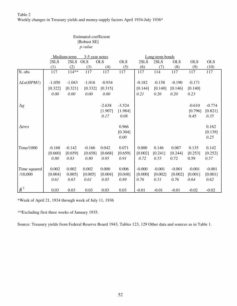
52

Table 2Weekly changes in Treasury yields and money-supply factors April 1934-July 1936*

Estimated coefficient [Robust SE] p-value

Medium-term 3-5 year notes Long-term bonds 2SLS 2SLS OLS OLS OLS 2SLS 2SLS OLS OLS OLS

(1) (2) (3) (4) (5) (6) (7) (8) (9) (10)

N. obs 117 114** 117 117 117 117 114 117 117 117

∆Ln(HPM1) -1.050 -1.043 -1.016 -0.934 -0.182 -0.158 -0.190 -0.171

[0.322] [0.321] [0.332] [0.315] [0.144] [0.140] [0.146] [0.140]

0.00 0.00 0.00 0.00 0.21 0.26 0.20 0.23

-2.638 -3.524 -0.610 -0.774∆g

[1.907] [1.984] [0.796] [0.821]

0.17 0.08 0.45 0.35

0.966 0.162∆tres

[0.304] [0.139]

0.00 0.25

Time/1000 -0.168 -0.142 -0.166 0.042 0.071 0.000 0.146 0.087 0.135 0.142

[0.660] [0.659] [0.658] [0.668] [0.659] [0.002] [0.241] [0.244] [0.253] [0.252]

0.80 0.83 0.80 0.95 0.91 0.72 0.55 0.72 0.59 0.57

Time squared 0.002 0.002 0.002 0.000 0.006 -0.000 -0.001 -0.001 -0.001 -0.001

/10,000 [0.004] 0.005] [0.005] [0.004] [0.048] [0.000] [0.002] [0.002] [0.001] [0.001]

0.61 0.65 0.61 0.85 0.89 0.76 0.51 0.76 0.64 0.62

0.03 0.03 0.03 0.03 0.03 -0.01 -0.01 -0.01 -0.02 -0.02R2

*Week of April 21, 1934 through week of July 11, 1936

**Excluding first three weeks of January 1935.

Source: Treasury yields from Federal Reserve Board 1943, Tables 123, 129 Other data and sources as in Table 1.

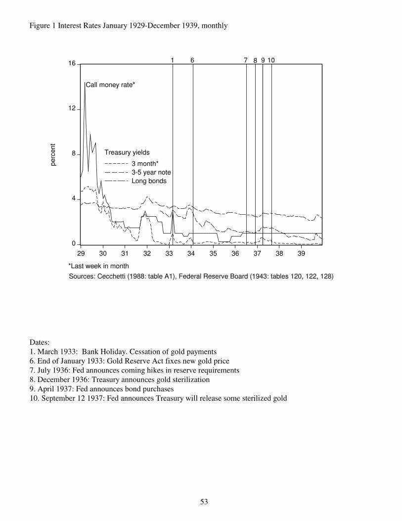
53

0

4

8

12

16

29 30 31 32 33 34 35 36 37 38 39

3 month*

3-5 year note

Long bonds

Call money rate*

Treasury yields

Sources: Cecchetti (1988: table A1), Federal Reserve Board (1943: tables 120, 122, 128)

1 6 7 8 9 10perc

ent

*Last week in month

Figure 1 Interest Rates January 1929-December 1939, monthly

Dates:1. March 1933: Bank Holiday. Cessation of gold payments6. End of January 1933: Gold Reserve Act fixes new gold price7. July 1936: Fed announces coming hikes in reserve requirements8. December 1936: Treasury announces gold sterilization9. April 1937: Fed announces bond purchases10. September 12 1937: Fed announces Treasury will release some sterilized gold

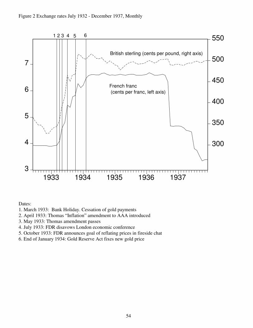
54

3

4

5

6

7

300

350

400

450

500

550

1933 1934 1935 1936 1937

1 2 3 4 5 6

British sterling (cents per pound, right axis)

French franc (cents per franc, left axis)

Figure 2 Exchange rates July 1932 - December 1937, Monthly

Dates:1. March 1933: Bank Holiday. Cessation of gold payments2. April 1933: Thomas “Inflation” amendment to AAA introduced3. May 1933: Thomas amendment passes4. July 1933: FDR disavows London economic conference5. October 1933: FDR announces goal of reflating prices in fireside chat6. End of January 1934: Gold Reserve Act fixes new gold price

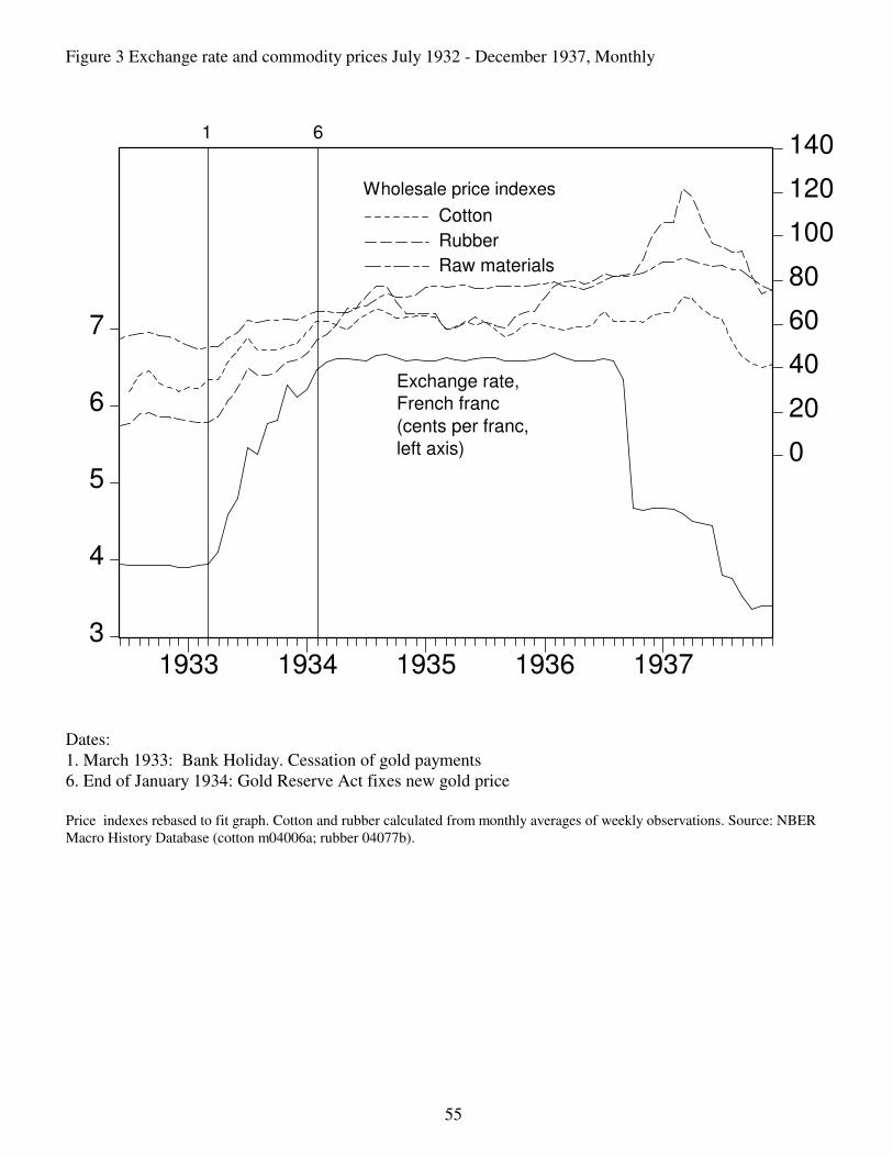
55

3

4

5

6

7

0

20

40

60

80

100

120

140

1933 1934 1935 1936 1937

Cotton

Rubber

Raw materials

Exchange rate,French franc

(cents per franc,left axis)

1 6

Wholesale price indexes

Figure 3 Exchange rate and commodity prices July 1932 - December 1937, Monthly

Dates:1. March 1933: Bank Holiday. Cessation of gold payments6. End of January 1934: Gold Reserve Act fixes new gold price

Price indexes rebased to fit graph. Cotton and rubber calculated from monthly averages of weekly observations. Source: NBERMacro History Database (cotton m04006a; rubber 04077b).

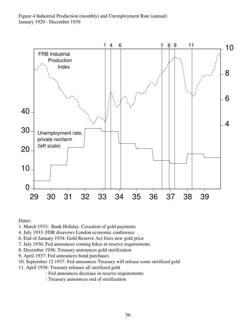
56

0

10

20

30

40

4

6

8

10

29 30 31 32 33 34 35 36 37 38 39

Unemployment rate,

private nonfarm

(left scale)

1 4 6 7 8 9 11

FRB Industrial

Production

Index

Figure 4 Industrial Production (monthly) and Unemployment Rate (annual)January 1929 - December 1939

Dates:1. March 1933: Bank Holiday. Cessation of gold payments4. July 1933: FDR disavows London economic conference6. End of January 1934: Gold Reserve Act fixes new gold price7. July 1936: Fed announces coming hikes in reserve requirements8. December 1936: Treasury announces gold sterilization9. April 1937: Fed announces bond purchases10. September 12 1937: Fed announces Treasury will release some sterilized gold11. April 1938: Treasury releases all sterilized gold : Fed announces decrease in reserve requirements : Treasury announces end of sterilization

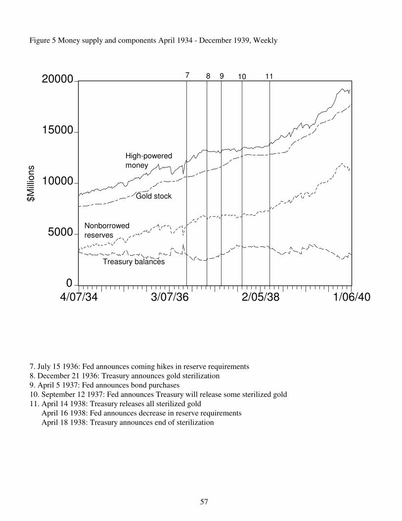
57

0

5000

10000

15000

20000

4/07/34 3/07/36 2/05/38 1/06/40

$M

illio

ns

7 8 9 10 11

High-powered

money

Gold stock

Nonborrowed

reserves

Treasury balances

Figure 5 Money supply and components April 1934 - December 1939, Weekly

7. July 15 1936: Fed announces coming hikes in reserve requirements8. December 21 1936: Treasury announces gold sterilization9. April 5 1937: Fed announces bond purchases10. September 12 1937: Fed announces Treasury will release some sterilized gold11. April 14 1938: Treasury releases all sterilized gold April 16 1938: Fed announces decrease in reserve requirements April 18 1938: Treasury announces end of sterilization

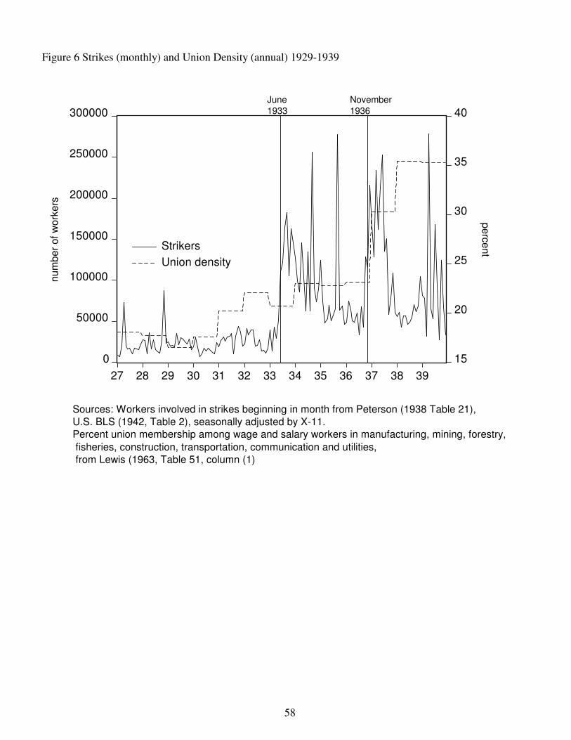
58

0

50000

100000

150000

200000

250000

300000

15

20

25

30

35

40

27 28 29 30 31 32 33 34 35 36 37 38 39

Strikers

Union density

June1933

pe

rce

nt

Sources: Workers involved in strikes beginning in month from Peterson (1938 Table 21),U.S. BLS (1942, Table 2), seasonally adjusted by X-11.Percent union membership among wage and salary workers in manufacturing, mining, forestry,

fisheries, construction, transportation, communication and utilities, from Lewis (1963, Table 51, column (1)

nu

mb

er

of w

ork

ers

November1936

Figure 6 Strikes (monthly) and Union Density (annual) 1929-1939

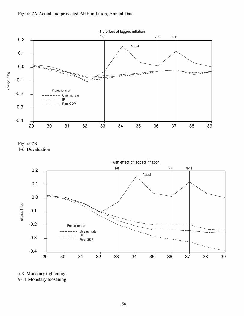
59

-0.4

-0.3

-0.2

-0.1

0.0

0.1

0.2

29 30 31 32 33 34 35 36 37 38 39

Unemp. rate

IP

Real GDP

No effect of lagged inflation

Actual

Projections on

1-6 7,8 9-11

change in log

-0.4

-0.3

-0.2

-0.1

0.0

0.1

0.2

29 30 31 32 33 34 35 36 37 38 39

Unemp. rate

IP

Real GDP

with effect of lagged inflation

Actual

Projections on

1-6 7,8 9-11

change in log

Figure 7A Actual and projected AHE inflation, Annual Data

Figure 7B1-6 Devaluation

7,8 Monetary tightening9-11 Monetary loosening

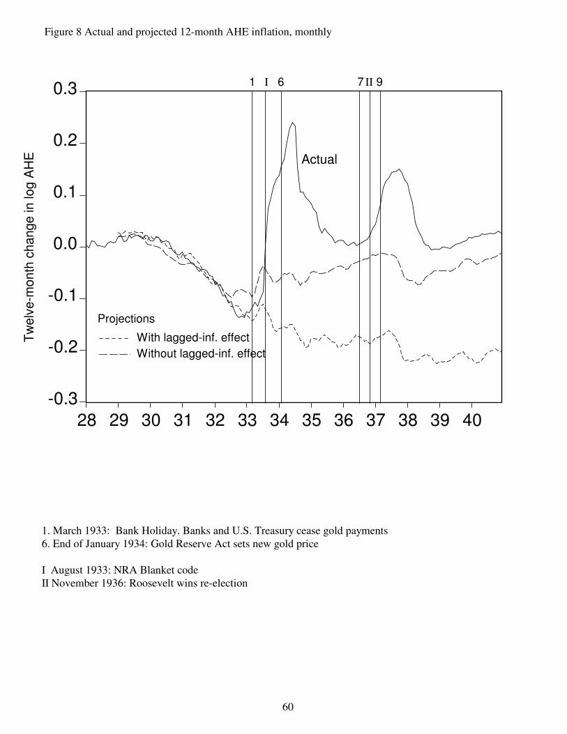
60

-0.3

-0.2

-0.1

0.0

0.1

0.2

0.3

28 29 30 31 32 33 34 35 36 37 38 39 40

With lagged-inf. effect

Without lagged-inf. effect

Actual

Tw

elv

e-m

onth

change in log A

HE

1 6 7 9

Projections

I II

Figure 8 Actual and projected 12-month AHE inflation, monthly

1. March 1933: Bank Holiday. Banks and U.S. Treasury cease gold payments6. End of January 1934: Gold Reserve Act sets new gold price

I August 1933: NRA Blanket codeII November 1936: Roosevelt wins re-election

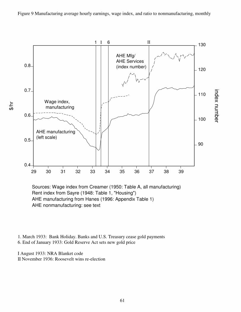
61

0.4

0.5

0.6

0.7

0.8

90

100

110

120

130

29 30 31 32 33 34 35 36 37 38 39

AHE manufacturing(left scale)

Wage index, manufacturing$

/hr

index n

um

ber

Sources: Wage index from Creamer (1950: Table A, all manufacturing)

Rent index from Sayre (1948: Table 1, "Housing")

AHE manufacturing from Hanes (1996: Appendix Table 1)

AHE nonmanufacturing: see text

1 6

AHE Mfg/AHE Services(index number)

I II

Figure 9 Manufacturing average hourly earnings, wage index, and ratio to nonmanufacturing, monthly

1. March 1933: Bank Holiday. Banks and U.S. Treasury cease gold payments6. End of January 1933: Gold Reserve Act sets new gold price

I August 1933: NRA Blanket code II November 1936: Roosevelt wins re-election