Copyright © 2013, 2014, 2015 by John Y. Campbell, Carolin Pflueger, and Luis M. Viceira

Working papers are in draft form. This working paper is distributed for purposes of comment and discussion only. It may not be reproduced without permission of the copyright holder. Copies of working papers are available from the author.

Monetary Policy Drivers of Bond and Equity Risks John Y. Campbell Carolin Pflueger Luis M. Viceira

Working Paper

14-031 June 15, 2015

Monetary Policy Drivers of Bond and Equity Risks

John Y. Campbell, Carolin Pflueger, and Luis M. Viceira1

First draft: March 2012This draft: June 2015

1Campbell: Department of Economics, Littauer Center, Harvard University, Cambridge MA 02138,USA, and NBER. Email john campbell@harvard.edu. Pflueger: University of British Columbia, VancouverBC V6T 1Z2, Canada. Email carolin.pflueger@sauder.ubc.ca. Viceira: Harvard Business School, BostonMA 02163 and NBER. Email lviceira@hbs.edu. We are grateful to Alberto Alesina, Fernando Alvarez,Yakov Amihud, Gadi Barlevy, Robert Barro, Charlie Bean, Paul Beaudry, Philip Bond, Mikhail Chernov,George Constantinides, Alexander David, Ian Dew-Becker, Adlai Fisher, Ben Friedman, Lorenzo Garlappi,Joao Gomes, Joshua Gottlieb, Gita Gopinath, Robin Greenwood, Lars Hansen, Christian Julliard, AnilKashyap, Ralph Koijen, Howard Kung, Leonid Kogan, Deborah Lucas, Greg Mankiw, Lubos Pastor, HaraldUhlig, Pietro Veronesi, Michael Woodford, conference and seminar participants at the University of BritishColumbia, the Bank of Canada, Universidad Carlos III, the University of Calgary, the University of Chicago,the Chicago Booth Finance Lunch Seminar, the Federal Reserve Bank of Chicago, the Federal Reserve Bankof New York, the Harvard Monetary Economics Seminar, the 2013 HBS Finance Research Retreat, IESE,LSE, LBS, the University of Miami, MIT Sloan, NYU Stern School, the Vienna Graduate School of Finance,ECWFC 2013, PNWCF 2014, the Jackson Hole Finance Conference 2014, the ASU Sonoran Winter FinanceConference 2014, the Duke/UNC Asset Pricing Workshop, the Monetary Policy and Financial MarketsConference at the Federal Reserve Bank of San Francisco, the Adam Smith Asset Pricing Workshop, theSFS Cavalcade 2014, and especially our discussants Jules van Binsbergen, Olivier Coibion, Gregory Duffee,Martin Lettau, Francisco Palomino, Monika Piazzesi, Rossen Valkanov, and Stanley Zin for helpful commentsand suggestions. We thank Jiri Knesl and Alex Zhu for able research assistance. This material is based uponwork supported by Harvard Business School Research Funding and the PH&N Centre for Financial Researchat UBC.

Abstract

How do monetary policy rules, monetary policy uncertainty, and macroeconomic shocksaffect the risk properties of US Treasury bonds? The exposure of US Treasury bonds to thestock market has moved considerably over time. While it was slightly positive on averageover the period 1960-2011, it was unusually high in the 1980s, and negative in the 2000s, aperiod during which Treasury bonds enabled investors to hedge macroeconomic risks. Thispaper develops a New Keynesian macroeconomic model with habit formation preferencesthat prices both bonds and stocks. The model attributes the increase in bond risks in the1980s to a shift towards strongly anti-inflationary monetary policy, while the decrease inbond risks after 2000 is attributed to a renewed focus on output fluctuations, and a shiftfrom transitory to persistent monetary policy shocks. Endogenous responses of bond riskpremia amplify these effects of monetary policy on bond risks.

1 Introduction

In different periods of history, long-term US Treasury bonds have played very different

roles in investors’ portfolios. During the Great Depression of the 1930s, and once again

in the first decade of the 21st Century, Treasury bonds served to hedge other risks that

investors were exposed to: the risk of a stock market decline, and more generally the risk

of a weak macroeconomy, with low output and high unemployment. Treasuries performed

well both in the Great Depression and in the two recessions of the early and late 2000s.

During the 1970s and especially the 1980s, however, Treasury bonds added to investors’

macroeconomic risk exposure by moving in the same direction as the stock market and

the macroeconomy. A number of recent papers including Baele, Bekaert, and Inghelbrecht

(2010), Campbell, Sunderam, and Viceira (2013), Christiansen and Ranaldo (2007), David

and Veronesi (2013), Guidolin and Timmermann (2006), and Viceira (2012) have documented

these developments. These stylized facts raise the question what macroeconomic forces

determine the risk properties of US Treasury bonds, and particularly their changes over

time.

The contribution of this paper is twofold. First, we develop a model combining a stan-

dard New Keynesian macroeconomy with habit formation preferences. Bonds and stocks in

the model can be priced from assumptions about their payoffs. Second, we use the model

to relate changes in bond risks to periodic regime changes in the parameters of the cen-

tral bank’s monetary policy rule and the volatilities of macroeconomic shocks, including a

regime shift that we identify in the early 2000s. Since monetary policy in our model affects

macroeconomic and risk premium dynamics, we capture both the direct and indirect effects

of monetary policy changes.

Macroeconomic dynamics in our model follow a standard three-equation New Keynesian

1

model. An investment-saving curve (IS) describes real equilibrium in the goods market based

on the Euler equation of a representative consumer, a Phillips curve (PC) describes the effects

of nominal frictions on inflation, and a monetary policy reaction function (MP) embodies

a Taylor rule as in Clarida, Gali, and Gertler (1999), Taylor (1993), and Woodford (2001).

A time-varying inflation target in the monetary policy rule captures investors’ long-term

perceived policy target and volatility in long-term bond yields.

While we model macroeconomic dynamics as loglinear, preferences in our model are

nonlinear to capture time-varying risk premia in bonds and stocks. As in Campbell and

Cochrane (1999), habit formation preferences generate highly volatile equity returns and

address the “equity volatility puzzle” one of the leading puzzles in consumption-based asset

pricing (Campbell, 2003). In contrast to Campbell and Cochrane (1999), our preferences are

consistent with an exactly loglinear consumption Euler equation, time-varying conditionally

homoskedastic real interest rates, and endogenous macroeconomic dynamics. The model is

overall successful at matching the comovement of bond and stock returns, while generating

time-varying bond and equity risk premia.

By using a New Keynesian macroeconomic framework, in which price stickiness allows

monetary policy to have real effects, we overcome some of the limitations of affine term

structure and real business cycle approaches. One common approach to studying macroe-

conomic bond risks is to use identities that link bond returns to movements in bond yields,

and that link nominal bond yields to expectations of future short-term real interest rates,

expectations of future inflation rates, and time-varying risk premia on longer-term bonds

over short-term bonds. Barsky (1989), Shiller and Beltratti (1992), and Campbell and Am-

mer (1993) were early examples of this approach. A more recent literature has proceeded

in a similar spirit, building on the no-arbitrage restrictions of affine term structure models

2

(Duffie and Kan 1996, Dai and Singleton 2000, 2002, Duffee 2002) to estimate multifactor

term structure models with both macroeconomic and latent factors (Ang and Piazzesi 2003,

Ang, Dong, and Piazzesi 2007, Rudebusch and Wu 2007). Although these exercises can be

informative, they are based on a reduced-form econometric representation of the stochastic

discount factor and the process driving inflation. This limits the insights they can deliver

about the underlying macroeconomic determinants of bond risks.

A more ambitious approach is to build a general equilibrium model of bond pricing. Real

business cycle models have an exogenous real economy, driven by shocks to either goods en-

dowments or production, and an inflation process that is either exogenous or driven by

monetary policy reactions to the real economy. Papers in the real business cycle tradition

often assume a representative agent with Epstein-Zin preferences, and generate time-varying

bond risk premia from stochastic volatility in the real economy and/or the inflation pro-

cess (Song 2014, Bansal and Shaliastovich 2013, Buraschi and Jiltsov 2005, Burkhardt and

Hasseltoft 2012, Gallmeyer et al 2007, Piazzesi and Schneider 2006). Some papers in-

stead derive time-varying risk premia from habit formation in preferences, with or without

stochastic macroeconomic volatility (Ermolov 2015, Bekaert, Engstrom, and Grenadier 2010,

Bekaert, Engstrom, and Xing 2009, Buraschi and Jiltsov 2007, Dew-Becker 2013, Wachter

2006). Under either set of assumptions, this work allows only a more limited role for mone-

tary policy, which determines inflation (at least in the long run) but has no influence on the

real economy.2

Our model is most closely related to a recent literature exploring the asset pricing impli-

cations of New Keynesian models. Recent papers in this literature include Andreasen (2012),

Bekaert, Cho, and Moreno (2010), Van Binsbergen et al (2012), Dew-Becker (2014), Kung

2A qualification to this statement is that in some models, such as Buraschi and Jiltsov (2005), a nominaltax system allows monetary policy to affect fiscal policy and, through this indirect channel, the real economy.

3

(2015), Li and Palomino (2014), Palomino (2012), Rudebusch and Wu (2008), and Rude-

busch and Swanson (2012). While this literature has begun to focus on the term structure

of interest rates, an integrated treatment of bonds and stocks, especially with risk premia

not driven by counterfactually extreme heteroskedasticity in macroeconomic fundamentals,

has so far proved elusive.3

We use our model to quantitatively investigate two candidate explanations for the empir-

ical instability in bonds’ risk properties: changes in monetary policy or changes in macroe-

conomic shocks. In this way we contribute to the literature on monetary policy regime shifts

(Andreasen 2012, Ang, Boivin, Dong, and Kung 2011, Bikbov and Chernov 2013, Boivin

and Giannoni 2006, Chib, Kang, and Ramamurthy 2010, Clarida, Gali, and Gertler 1999,

Palomino 2012, Rudebusch and Wu 2007, Smith and Taylor 2009). While this literature

has begun to focus on the implications of monetary regime shifts for the term structure of

interest rates, previous papers have not looked at the implications for the comovements of

bonds and equities as we do here. Our structural analysis takes account of various channels

by which the monetary policy regime affects the sensitivities of bond and stock returns to

macroeconomic shocks, including endogenous responses of risk premia.4

Both US monetary policy and the magnitude of macroeconomic shocks have changed

substantially over our sample from 1960 to 2011. Testing for break dates in the relation

between the Federal Funds rate, output, and inflation, we determine three distinct monetary

policy regimes. The first regime comprises the period of rising inflation in the 1960s and

3In contrast, several papers have used reduced-form affine or real business cycle models to provide anintegrated treatment of bonds and stocks (Ang and Ulrich 2012, Bansal and Shaliastovich 2013, Bekaert,Engstrom, and Grenadier 2010, Ermolov 2015, Koijen, Lustig, and Van Nieuwerburgh 2010, Campbell 1986,Campbell, Sunderam, and Viceira 2013, d’Addona and Kind 2006, Dew-Becker 2013, Eraker 2008, Hasseltoft2009, Lettau and Wachter 2011, Wachter 2006).

4Song (2014), in a paper circulated after the first version of this paper, considers bond-stock comovementsin a model with exogenous real dynamics.

4

1970s, while the second one covers the inflation-fighting period under Federal Reserve Board

chairmen Paul Volcker and Alan Greenspan. The third regime is characterized by renewed

attention to output stabilization and smaller, but more persistent, shocks to the monetary

policy rule. If central bank policy affects the macroeconomy through nominal interest rates,

it is natural to think that these significant changes in monetary policy should change the

risks of bonds and stocks.

The nature of economic shocks has also changed over time, with potentially important

implications for bond risks. While oil supply shocks were prominent during the 1970s and

early 1980s, they became less important during the subsequent Great Moderation. In our

model, Phillips curve shocks act as supply shocks, leading to high inflation recessions. Nom-

inal bond prices fall with rising inflation expectations, while stock prices fall with recessions,

so Phillips curve shocks move bonds and stocks in the same direction and give rise to positive

nominal bond betas. In contrast, credible shocks to the central bank’s long-term inflation

target, or equivalently persistent shocks to the monetary policy rule, reduce the beta of

nominal bonds. A downward drift in the perceived target drives down inflation and induces

firms with nominal rigidities to reduce output. Consequently, a negative target shock raises

the value of nominal bonds just as equity prices fall, decreasing the stock-market beta of

nominal bonds.

Figure 1 shows a timeline of changing US bond risks, together with estimated monetary

policy regimes, and oil price shocks from Hamilton (2009). We estimate monetary policy

break dates using data on the Federal Funds rate, the output gap (the gap between real out-

put and potential output under flexible prices), and inflation.5 The statistically determined

dates 1977Q2 and 2001Q1 line up remarkably closely with changes in bond betas and institu-

5For details on the econometric procedure, see Section 3.

5

tional and personal changes at the Federal Reserve, even if a reading of US Federal Reserve

history might suggest a slightly later first break date. The 1977Q2 break date precedes by

two years Paul Volcker’s appointment as Federal Reserve chairman, a change that ushered

in a new era of inflation fighting. The second break date corresponds to the end of the

great economic expansion in the 1990s and the start of the Federal Reserve’s accommodative

response to the end of the technology boom and the attacks of 9/11.

The 5-year nominal bond CAPM betas and return volatilities plotted in Figure 1 illustrate

important changes in the risks of nominal bonds over time.6 Moreover, changes in nominal

bond risks broadly line up with changes in monetary policy regimes. The nominal bond beta,

shown in Panel A, was positive but close to zero before 1977, strongly positive thereafter, and

turned negative after the year 2000. Bond return volatility, shown in Panel B, also increased

during the middle subperiod, although there is higher-frequency variation as well, most

notably a short-lived spike in the early 1980s. In contrast, oil price shocks are concentrated

in the first two of our subperiods and there is no visually apparent relation between oil price

shocks and nominal bond betas. The main empirical analysis in this paper systematically

examines the role of time-varying shock volatilities and finds that they interact with monetary

policy in important ways to jointly determine the risks of nominal bonds.

The organization of the paper is as follows. Section 2 describes the model for macroe-

conomic dynamics and preferences. This section also derives the New Keynesian IS curve

from habit preferences.

Section 3 describes our data sources and presents summary statistics for our full sam-

ple period, 1954Q3 through 2011Q4, and for three subperiods, 1960Q2–1977Q1, 1977Q2–

2000Q4, and 2001Q1–2011Q4. For each subperiod, this section also estimates a reduced-form

6We show filtered CAPM betas and standard deviations of daily returns on a benchmark 5-year nominalbond over a rolling 3-month window, together with 95% confidence intervals.

6

monetary policy rule and backs out naıve estimates of Taylor rule parameters. These naıve

monetary policy parameter estimates, unlike estimates from our full model, do not account

for regression bias caused by endogeneity of macroeconomic variables and time-variation in

the central bank’s inflation target.

Section 4 calibrates our model to fit both macroeconomic and asset pricing data over our

three subperiods. The model fits bond-stock comovements and empirical Taylor-rule type

regressions for each subperiod, while generating plausible consumption growth volatility

and equity and bond risk premia. Section 5 presents counterfactual analysis, asking how

bond risks would have evolved over time if the monetary policy rule, or the volatilities of

macroeconomic shocks, had been stable instead of time-varying. Section 6 concludes, and

an online appendix (Campbell, Pflueger, and Viceira 2015) presents additional details.

2 A New Keynesian Asset Pricing Model

Our model integrates a standard three-equation loglinear New Keynesian macroeconomic

model with a habit-formation model of asset prices. While many variants of the basic New

Keynesian model have been proposed, we use a small-scale New Keynesian framework to

study the key implications of the broader class of New Keynesian models for asset prices.7 We

abstract from nonlinearities in macroeconomic dynamics in order to focus on nonlinearities

in asset prices, where they are most salient. On the asset pricing side, we build on the habit

model of Campbell and Cochrane (1999). The stochastic discount factor (SDF) links asset

returns and macroeconomic and monetary variables in equilibrium.

The Euler equation is a standard New Keynesian building block and provides an equiv-

7Woodford (2003) argues that the three-equation log-linearized New Keynesian model captures many ofthe key dynamics of more complicated models, including models with investment.

7

alent of the investment-savings (IS) curve. We derive a habit-founded Euler equation in

terms of the current, lagged, and expected output gaps and the short-term real interest rate.

Euler equations with both backward-looking and forward-looking components are common

in the dynamic stochastic general equilibrium (DSGE) literature (Christiano, Eichenbaum,

and Evans 2005, Boivin and Giannoni 2006, Smets and Wouters 2007).8 The backward-

looking component is important for obtaining a unique equilibrium (Cochrane 2011) and

for capturing the empirical output response to monetary policy shocks (Fuhrer 2000). The

forward-looking component follows from standard household dynamic optimization.

The second building block of a New Keynesian model is the Phillips curve (PC) equation

that links inflation and real output in equilibrium. We directly assume a PC with both

forward- and backward-looking components, as may arise from different microfoundations

for nominal rigidities. In the appendix, we derive a PC for firms that face Calvo (1983) price-

setting frictions and partial indexing as in Smets and Wouters (2003), and maximize future

expected profits discounted with our SDF. Alternative microfoundations, such as infrequent

information updating, may yield variants of this benchmark PC (Mankiw and Reis 2002).

The third building block of the model is an equation describing the behavior of the cen-

tral bank. We assume that the central bank’s policy instrument is the short-term nominal

interest rate. The central bank sets this interest rate according to a Taylor (1993) monetary

policy (MP) rule, as a linear function of the “inflation gap” (the deviation of inflation from

the central bank’s target), the output gap, and the lagged nominal interest rate. Empiri-

8Christiano, Eichenbaum, and Evans (2005) and Boivin and Giannoni (2006) derive a backward- andforward-looking linearized Euler equation in a model where utility depends on the difference between con-sumption and an internal habit stock. A backward-looking component in the Euler equation can also bederived in a model with multiplicative external habit (Abel 1990, Fuhrer 2000). Our model differs from theseprevious works in that difference habit in our model gives rise to time-varying bond and equity risk premia.Rudebusch and Swanson (2008) allow for time-varying risk premia in a production-based model. However,their focus is on the endogenous labor response to habits and they use perturbation solution methods, whichwe have found not to work well for our model.

8

cally, the Fed appears to smooth interest rates over time, and we capture this by modeling

the nominal short rate as adjusting gradually to the target rate. This approach is fairly

standard in the New Keynesian literature, although there is some debate over the relative

importance of partial adjustment and serially correlated unobserved fundamentals in the MP

rule (Rudebusch 2002, Coibion and Gorodnichenko 2012).

While our preferences build on Campbell and Cochrane (1999) and Wachter (2006), they

differ in that surplus consumption—or consumption relative to habit—can depend on the

current and lagged output gaps. As a result, the consumption Euler equation takes the form

of an exactly loglinear New Keynesian Euler equation depending on current, future, and

lagged output gaps as in Clarida, Gali, and Gertler (1999, CGG). Risk premia increase when

surplus consumption and the output gap are low, consistent with the empirical evidence on

stock and bond return predictability (Chen 1991, Cochrane 2007, Cochrane and Piazzesi

2005, Fama 1990, Fama and French 1989, Lamont 1998, Lettau and Ludvigson 2001).

The New Keynesian macroeconomic model provides equilibrium dynamics for the output

gap, inflation, and the policy rate, but preferences are over consumption. We bridge this

gap between the macroeconomic and asset pricing sides of the model by assuming that

consumption and the output gap are driven by the same shock. We model the output gap as

the difference between current period consumption and an exponentially-weighted moving

average of lagged consumption. This specification generates near random-walk dynamics for

consumption, similar to the endowment consumption dynamics in Campbell and Cochrane

(1999), while preserving stationarity for the output gap.

Figure 2, Panel A supports this description of the joint dynamics of consumption and

the output gap. The figure plots the time series of stochastically detrended consumption—

log real consumption of nondurables and services less an exponentially-weighted moving

9

average with a half life of 2.6 years—and the log output gap. The two series move very

closely together—almost surprisingly so given the measurement issues in both series—with

a correlation of 90%.

We allow for shocks to the central bank’s long-run policy rate. These shocks can tem-

porarily boost demand in our model. We interpret them broadly as capturing persistent

shocks to expected policy rates, or explicit and perceived changes in the long-run inflation

target. As such, movements in the policy target capture changes in forward-looking public

expectations of central bank behavior, that are accompanied by almost no movement in

the Fed Funds rate. The central bank’s ability to steer output and inflation through target

expectations may vary with central bank credibility (Orphanides and Williams 2004).

We model the policy target rate as a unit root process, consistent with the extremely

high persistence in US inflation data (Ball and Cecchetti 1990, Stock and Watson 2007).

We choose a unit root specification rather than a highly persistent mean-reverting inflation

target for several reasons. First, the inflation target reflects consumers’ long-run target

expectations, whose changes cannot be anticipated. A mean-reverting inflation target would

imply counterintuitive predictability of target changes. Second, a highly persistent inflation

target may lead to equilibrium existence and uniqueness issues, while we can factor out a

unit root inflation target from equilibrium dynamics. Finally, while our unit root assumption

means that the unconditional variance of nominal interest rates is undefined, we believe

that this difficulty is driven by high empirical persistence in nominal bond yields rather

than our specific modeling assumption. Even with a highly persistent inflation target this

unconditional variance would be extremely sensitive to an imprecisely identified persistence

parameter.

Following CGG, we assume that transitions from one regime to another are structural

10

breaks, completely unanticipated by investors. We show in the appendix that model im-

plications are unchanged if we include a small, constant regime-switching probability. The

qualitative and quantitative implications from a model with unanticipated regime changes

survive for two reasons. First, quarterly transition probabilities have to be small to match

average empirical regime durations of ten to 25 years. Second, our regimes differ in an

important dimension from the model of David and Veronesi (2013), where learning about

regimes has important effects on bond and equity risks. David and Veronesi’s regimes are

characterized by exogenously given first moments for consumption growth and inflation. In

contrast, our regimes have identical long-run consumption growth and inflation distributions,

but differ endogenously in the co-movements of output, inflation, and interest rates. Thus

our approach can be regarded as complementary to David and Veronesi.

2.1 Macroeconomic dynamics

We model business cycle and inflation dynamics using a standard log-linearized three equa-

tion New Keynesian model (CGG):

xt = ρx−xt−1 + ρx+Etxt+1 − ψ(Etit − Etπt+1), (1)

πt = ρππt−1 + (1− ρπ)Etπt+1 + κxt + uPCt , (2)

it = ρiit−1 + (1− ρi) [γxxt + γπ (πt − π∗t ) + π∗t ] + uMPt , (3)

π∗t = π∗t−1 + u∗t . (4)

We denote the log output gap—the deviation of real output from flexible price equilibrium—

by xt and log inflation by πt. We write π∗t for the inflation target. We write it to denote the

log yield at time t—and return at time t + 1—on a one-period nominal T-bill. Similarly, rt

11

denotes the log yield on a one-period real Treasury bill. We use the subscript t for short-term

nominal and real interest rates to emphasize that they are known at time t.

We do not include an IS shock in the Euler equation (1) because we require the IS

equation to be consistent with the consumption Euler equation.9 The New Keynesian PC

(2) has parameters ρπ, determining the relative weight on past inflation and expected future

inflation, and κ governing the sensitivity of inflation to the output gap.

Equations (3) and (4) describe monetary policy. They determine the short-term nominal

interest rate with parameters ρi controlling the influence of past interest rates on current

interest rates, γx governing the reaction of the interest rate to the output gap, and γπ

governing the response of the interest rate to inflation relative to its target level π∗t . Equation

(4) specifies that the central bank’s policy target follows a random walk.

Monetary policy in our model does not react directly to long-term nominal bond yields

or stock prices, but only to macroeconomic determinants of these asset prices. However, a

persistent policy target shifts the term structure similarly to a level factor. In that sense,

our model is similar to models where the level factor of the nominal term structure directly

enters the central bank’s monetary policy function (Rudebusch and Wu 2007, 2008).

Finally, we assume that the vector of shocks is independently and conditionally normally

distributed with mean zero and diagonal variance-covariance matrix:

ut = [uPCt , uMPt , u∗t ]

′, Et−1 [utu′t] = Σu =

(σPC)2 0 0

0 (σMP )2 0

0 0 (σ∗)2

. (5)

9We found that modifying preferences to allow for an IS shock has little effect on the pricing of con-sumption claims.

12

Equation (5) has two important properties. First, the variances of all shocks in the model

are conditionally homoskedastic. The previous version of this paper generated countercycli-

cal risk premia from countercyclical volatility of shocks. While time-varying volatilities may

provide a convenient tool for generating time-varying risk premia, strong countercyclical het-

eroskedasticity is not a feature of macroeconomic data.10 The habit formation preferences

in this model reconcile conditionally homoskedastic macroeconomic fundamentals with em-

pirically plausible time-variation in bond and equity risk premia. Second, the assumption

that monetary policy shocks uMPt and u∗t are uncorrelated with PC shocks captures the

notion that all systematic variation in the short-term nominal interest rate is reflected in the

monetary policy rule.

2.2 Consumption and Preferences

Consider a habit formation model of the sort proposed by Campbell and Cochrane (1999),

where utility is a power function of the difference between consumption C and habit H:

Ut =(Ct −Ht)

1−γ − 1

1− γ=

(StCt)1−γ − 1

1− γ. (6)

Here St = (Ct − Ht)/Ct is the surplus consumption ratio and γ is a curvature parameter

that controls risk aversion. Relative risk aversion varies over time as an inverse function of

the surplus consumption ratio: −UCCC/UC = γ/St.

10We thank our discussants Jules van Binsbergen, Martin Lettau, and Monika Piazzesi for emphasizingthis point. Ermolov (2015), in a paper circulated after the previous version of this paper, also uses changingfundamental volatility to generate changing risk premia.

13

Marginal utility in this model is

U ′t = (Ct −Ht)−γ = (StCt)

−γ , (7)

and log marginal utility is given by lnU ′t = −γ(st + ct).

2.2.1 Modeling Consumption

We model consumption in terms of the output gap, so inflation and the Federal Funds rate

are relevant for consumption only to the extent that they are correlated with the output

gap. In small-scale New Keynesian models, it is common to model consumption as equal to

the output gap (CGG). However, the output gap is stationary while empirical consumption

appears to have a unit root, with potentially important asset pricing implications. For

constants τ and g, we model consumption as follows:

ct = gt+ τ (xt + (1− φ)[xt−1 + xt−2 + ...]) . (8)

For any stationary output gap process, the relation (8) defines a consumption process with a

unit root. As a leading example, if the output gap follows an AR(1) process with first-order

autocorrelation parameter φ, (8) implies that consumption follows a random walk with drift.

The parameter g regulates average consumption growth and τ regulates the relative volatility

of consumption and the output gap.

Ignoring constants, we can equivalently rewrite the output gap in terms of consumption

in excess of an exponentially decaying stochastic trend:

xt = τ−1 (ct − (1− φ)[ct−1 + φct−2 + ...]) . (9)

14

While our model of consumption and output is reduced form, it captures a salient feature

of the data. Both the left-hand and right-hand-sides in (9) are stationary, so it makes sense

to consider the correlation in the data. Figure 2, Panel A shows that stochastically detrended

real consumption and the log output gap (from the Congressional Budget Office) are 90%

correlated. We use an annualized smoothing parameter of φ = 0.94, corresponding to a half-

life of 2.6 years. Importantly, Figure 2 suggests a stable consumption-output gap relation

across monetary policy and shock regimes.

2.2.2 Modeling the Surplus Consumption Ratio

We specify the dynamics for log surplus consumption to satisfy the following two features.

First, we require log surplus consumption to be stationary, as in Campbell and Cochrane

(1999). Second, the loglinear Euler equation (1) is exact for our choice of preferences.

Denoting the demeaned log output gap by xt, unexpected consumption innovations by

εc,t+1, and the steady state log surplus consumption ratio by s, we assume the following

dynamics for the log surplus consumption ratio:

st+1 = (1− θ0)s+ θ0st + θ1xt + θ2xt−1 + λ(st)εc,t+1, (10)

εc,t+1 = ct+1 − Etct+1 = τ (xt+1 − Etxt+1) . (11)

We can use (9) to substitute out the output gap from (10) and re-write surplus consump-

tion dynamics in terms of current and lagged consumption (ignoring constants):

st+1 = θ0st + θ1τ−1 (ct − (1− φ) [ct−1 + φct−2 + ...])

+θ2τ−1 (ct−1 − (1− φ) [ct−2 + φct−3 + ...]) + λ(st)εc,t+1. (12)

15

When θ1 = θ2 = 0, the surplus consumption dynamics (10) are the same as in Campbell

and Cochrane (1999). In the appendix, we show that log habit can be approximated as

a distributed lag of log consumption, with weights on distant lags converging to those of

Campbell and Cochrane (1999). This distributed lag expression shows that θ1 and θ2 free up

how strongly log habit loads onto the first two lags of consumption, relative to Campbell and

Cochrane (1999). Increases in θ2 and θ2 reduce log habit loadings onto the most recent lags

of consumption, while increasing the loadings on medium-term lags. In the calibrated model,

we find that simulated log surplus consumption is closely related to the log output gap. A

regression of the simulated log surplus consumption ratio onto the output gap yields a slope

coefficient of around 12 and an R-squared of 63%, weighted across calibration periods.11

The specification (10) is similar in spirit to Wachter (2006). However, our approach has

several advantages in a model that endogenously derives macroeconomic dynamics. While

short-term real interest rates in Wachter (2006) and Menzly, Santos, and Veronesi (2004)

depend on the surplus consumption ratio and are therefore heteroskedastic, the short-term

real rate in our model depends on current, lagged, and future values of the output gap.

This allows us to obtain equilibrium dynamics for the output gap and consumption that

are conditionally homoskedastic—an assumption in Campbell and Cochrane (1999), Menzly,

Santos, and Veronesi (2004), and Wachter (2006). In addition, the dynamics (10) allow us to

derive exactly the loglinear New Keynesian Euler equation (1) from the consumption Euler

equation.

11If θ1 and θ2 are different from zero, there is the theoretical possibility that the log surplus consumptionratio exceeds the maximal value smax, where the sensitivity function is non-zero. However, the probabilityof this event is very small in our calibrated model (less than 0.1% per quarter). In this respect our model issimilar to Campbell and Cochrane (1999), who also have an upper bound on surplus consumption that cannever be crossed in continuous time.

16

2.2.3 Consumption Euler equation

Standard no-arbitrage conditions in asset pricing imply that the gross one-period real return

(1 +Rt+1) on any asset satisfies

1 = Et [Mt+1 (1 +Rt+1)] , (13)

where

Mt+1 =βU ′t+1

U ′t(14)

is the stochastic discount factor (SDF). The Euler equation for the return on a one-period

real T-bill can be written in log form as:

lnU ′t = rt + ln β + ln EtU′t+1. (15)

For simplicity, we assume that short-term nominal interest rates contain no risk premia

or that it = rt+Etπt+1, where πt+1 is inflation from time t to time t+1. This approximation

is justified if uncertainty about inflation is small at the quarterly horizon, as appears to be

the case empirically. Substituting rt = it − Etπt+1 into (15), and dropping constants to

reduce the notational burden, we have:

lnU ′t = (it − Etπt+1) + ln EtU′t+1. (16)

17

Substituting (10) into the Euler equation for the one-period real T-bill gives

rt = − ln β + γg + γθ2xt−1 + γ (θ1 − τφ)xt + γτEtxt+1

−γ(1− θ0)(st − s)−γ2σ2

c

2(1 + λ(st))

2 . (17)

Now, we use Campbell and Cochrane (1999)’s condition that the terms in (17) involving st

cancel, which imposes restrictions on the sensitivity function λ(st). Moreover, habit must be

predetermined at and near the steady state. These conditions ensure that the steady-state

surplus consumption ratio and the sensitivity function λ are given by

S = σc

√γ

1− θ0

, (18)

s = log(S), (19)

smax = s+ 0.5(1− S2), (20)

λ(st, S) =

1S

√1− 2(st − s)− 1 , st ≤ smax

0 , st ≥ smax

. (21)

We then re-arrange the Euler equation in terms of the current, lagged, and future log

output gaps and the short-term real interest rate rt, ignoring constants for simplicity:

xt =τ

τφ− θ1︸ ︷︷ ︸ρx+

Etxt+1 +θ2

τφ− θ1︸ ︷︷ ︸ρx−

xt−1 −1

γ(τφ− θ1)︸ ︷︷ ︸ψ

rt. (22)

Several points are worth noting about the IS curve (22). First, the asset pricing Euler

equation holds without shocks. Second, because θ1 > 0, θ2 > 0 and φ < 1, the coefficients

on the lagged output gap and the expected future output gap sum to more than one. Third,

the slope of the IS curve ψ does not equal the elasticity of intertemporal substitution (EIS)

18

of the representative consumer.

The lag coefficient ρx− in the IS curve (22) is non-zero whenever the lagged output gap

enters into surplus consumption (i.e. θ2 6= 0). Cochrane (2011) shows that solutions to

purely forward-looking New Keynesian models are typically ill-behaved. We therefore need

θ2 6= 0 to obtain a partly backward-looking Euler equation and well-behaved macroeconomic

dynamics.

2.3 Modeling bonds and stocks

We model stocks as a levered claim on consumption ct. We assume that log dividend growth

is given by:

∆dt = δ∆ct. (23)

We interpret δ as capturing a broad concept of leverage, including operational leverage.

The interpretation of dividends as a levered claim on consumption is common in the asset

pricing literature (Abel 1990, Campbell 1986, 2003). We maintain our previous simplifying

approximation that risk premia on one-period nominal bonds equal zero, but risk premia on

longer-term bonds are allowed to vary, so the expectations hypothesis of the term structure

of interest rates does not hold.

2.4 Model solution and stability

We first describe the solution for macroeconomic dynamics. The state variable dynamics

have a solution of the form

Yt = PYt−1 +Qut, (24)

19

where

Yt = [xt, πt, ıt]′, (25)

πt = πt − π∗t , (26)

ıt = it − π∗t . (27)

We solve for P ∈ R3×3 and Q ∈ R3×4 using the method of generalized eigenvectors (see e.g.

Uhlig 1999).

In principle, the model can have more than one solution. We only consider dynamically

stable solutions with all eigenvalues of P less than one in absolute value, yielding non-

explosive solutions for the output gap, inflation gap, and interest rate gap. Cochrane (2011)

argues that there is no economic rationale for ruling out solutions solely on the basis of an

explosive inflation path. In general, in our model an explosive solution for inflation is also

explosive for the output gap and the real interest rate. We find it reasonable to rule out

such solutions with explosive real dynamics.

The inclusion of backward-looking terms in the IS curve and PC implies that there exist

at most a finite number of dynamically stable equilibria of the form (24). This is true even

when the monetary policy reaction to inflation (γπ) is smaller than one, which usually leads to

an indeterminate equilibrium in highly stylized Keynesian models with only forward-looking

components (Cochrane 2011).

Next, we require all our equilibria to satisfy a battery of equilibrium selection criteria to

rule out unreasonable solutions and pick a unique solution. We require the solution to be

real-valued and “expectationally stable” (Evans 1985, 1986, McCallum 2003). Expectational

stability requires that for small deviations from rational expectations, the system returns to

20

the equilibrium. We also impose the solution selection criterion of Uhlig (1999), which is

closely related to the minimum state variable solution proposed by McCallum (2004).

While we formally model regimes as lasting an infinite period of time, one might think

that agents understand that the regime will have to end eventually, potentially arbitrarily

far in the future. We implement the Cho and Moreno (2011) criterion, which captures this

limiting case. This criterion, also used by Bikbov and Chernov (2013), has two appealing

interpretations. The first interpretation captures the notion that if monetary policy changes

slowly over time and those changes are fully anticipated, even monetary policy regimes with

weak inflation responses may have unique equilibria (Farmer, Waggoner, and Zha 2009).12

The Cho and Moreno (2011) criterion is equivalent to assuming that the system returns to

an equilibrium with all variables constant from period T ∗ onwards and then letting T ∗ go

to infinity. An alternative interpretation of the Cho and Moreno (2011) criterion is closely

related to expectational stability. If agents deviate from rational expectations and instead

have constant expectations, the system returns to the Cho and Moreno (2011) equilibrium.

The Appendix provides full details on the model solution and solution criteria.

2.5 Solutions for bond and stock returns

We solve numerically for bond prices and equity dividend-price ratios. On the numerical side,

this paper contributes by extending the value function iteration methodology of Wachter

(2005) to multiple state variables. We found that methods relying on analytic linear ap-

proximations to the sensitivity function λ (e.g. Lopez, Lopez-Salido, and Vazquez-Grande

2014), numerical higher-order perturbation methods (Rudebusch and Swanson 2008), and

12We thank Mikhail Chernov for pointing out to us that when rational agents anticipate a return to adifferent equilibrium, even regimes with an inflation reaction coefficient less than one can have a determinateequilibrium.

21

numerical global projection methods led to substantial approximation error. For our baseline

grid and simulation, it takes about 45 minutes to solve and simulate the model once for all

three subperiod calibrations. The model solution is therefore too slow for estimation, but

we can conduct grid searches over lower-dimensional parameter subsets.

Let P dnt/Dt denote the price-dividend ratio of a zero-coupon claim on the aggregate stock

market dividend at time t+n. The price-dividend ratio on the aggregate stock market then

equals the infinite sum of zero-coupon price-dividend ratios. The price of a zero-coupon

claim for the dividend at time t is given by P d0t/Dt = 1. For n ≥ 1, we solve for the n-period

price-dividend ratio numerically using the iteration

P dnt

Dt

= Et

[Mt+1

Dt+1

Dt

P dn−1,t+1

Dt+1

].

Denoting n-period real and nominal zero-coupon bond prices by Pn,t and P $n,t, one-period

bond prices are given by

P $1,t = exp(−ıt − π∗t − rf ), (28)

P1,t = exp(−ıt + Etπt+1 − rf ). (29)

For n > 1, zero-coupon bond prices follow the recursions:

Pn,t = Et [Mt+1Pn−1,t+1] , (30)

P $n,t = Et

[Mt+1 exp(−πt+1)P $

n−1,t+1

]. (31)

Since n-period zero-coupon nominal bond prices are proportional to exp(−nπ∗t ), we solve

numerically for scaled nominal bond prices exp(nπ∗t )P$n,t.

22

We solve over a five-dimensional grid of the surplus consumption ratio st, the lagged

output gap xt−1, and the scaled vector Yt. Yt scales and rotates the variables in Yt such

that shocks to Yt are independent standard normal and the first element of Yt is condition-

ally perfectly correlated with consumption innovations. The baseline solution grid uses 50

gridpoints for st spaced between −50 and smax, and two gridpoints along every dimension

of Yt at plus and minus two standard deviations from the unconditional mean. It also uses

two gridpoints for xt−1 ranging over all output gap values covered by the grid for xt. We

therefore have a total of 800 gridpoints. We use Gauss-Legendre 40-point quadrature to

integrate over consumption shocks, and 10-point quadrature for those dimensions of Yt that

are contemporaneously uncorrelated with the SDF. We evaluate price-dividend ratios and

bond prices between gridpoints using five-dimensional loglinear interpolation. Asset pricing

properties are unchanged if we increase the grid size for any of these dimensions, indicating

that the baseline grid is sufficient.

2.6 Properties of bond and stock returns

The solutions for bond and stock returns imply that returns are conditionally heteroskedas-

tic (even though macroeconomic fundamentals are homoskedastic by assumption), and that

conditional expected asset returns vary over time with the surplus consumption ratio. Time-

varying risk premia generate a non-linear effect of fundamental shocks on bond betas which

can amplify their linear effect. For example, consider a contractionary shock that simulta-

neously lowers output and inflation. The shock pushes bond valuations higher and stock

valuations lower, generating a negative nominal bond beta. But the negative bond beta im-

plies that nominal bonds are safe. The increase in risk aversion following the contractionary

shock makes nominal bonds more valuable hedges, driving up their prices and making the

23

bond beta even more negative. We show in our calibration that amplification through time-

varying risk premia can be quantitatively important.

3 Preliminary Empirical Analysis

3.1 Monetary policy regimes

We explore monetary policy in three subperiods, which we determine using a Quandt Like-

lihood Ratio (QLR) test. The resulting break dates correspond closely to changes in bond

betas in Figure 1, a potentially alternative criterion for determining breaks. Our first sub-

period, 1960Q2–1977Q1, covers roughly the Fed chairmanships of William M. Martin and

Arthur Burns. The second subperiod, 1977Q2–2000Q4, covers the Fed chairmanships of

G. William Miller, Paul Volcker, and Alan Greenspan until the end of the long economic

expansion of the 1990s. The third subperiod, 2001Q1-2011Q4, contains the later part of

Greenspan’s chairmanship and the earlier part of Ben Bernanke’s chairmanship.13

Our identification of a third regime for monetary policy is supported by several observa-

tions. First, in the late 1990s and 2000s the Federal Reserve has placed increased emphasis

on transparency and providing guidance to market expectations, in part through changing

the policy rate gradually (Coibion and Gorodnichenko 2012, Stein and Sunderam 2015). As

a result of greater transparency and credibility, the central bank may have been able to

affect the real economy not only through immediate changes in the Fed Funds rate, as in

the earlier periods, but also through expectations of future changes. In our model, inflation

13Sims and Zha (2006) argue for a break in the volatility of money demand shocks in 2000 and a breakin the monetary policy rule in 1987. In the appendix, we show that the main findings in the paper arerobust to assuming a break in the monetary policy rule in 1987 and a break in volatilities of shocks in 2000.With these alternative break dates, the model attributes changes in bond betas around 2000 to changes inmonetary policy, and especially the volatilities of inflation target and monetary policy shocks.

24

target shocks can capture credible central bank announcements of future actions that are

not accompanied by any immediate rate changes.

Second, the experience of moderate inflation and apparently well anchored inflation ex-

pectations from the mid-1980s through the mid-1990s seems to have encouraged the Federal

Reserve to turn its attention back to output stabilization, after the single-minded focus on

combating inflation under Fed chairman Paul Volcker. Rigobon and Sack’s (2003) empirical

evidence is also consistent with this interpretation.

Illustrating both investors’ focus on the central bank’s output response and the forward-

looking nature of monetary policy in the 2000s, a typical New York Times bond market

commentary argued in 2000: “Prices of Treasury securities were down (...), after a stronger-

than-expected gain in industrial production raised investor concern about further interest

rate increases by the Federal Reserve.”14

3.2 Data and summary statistics

We use quarterly US data on output, inflation, interest rates, and aggregate bond and stock

returns from 1954Q3 to 2011Q4. GDP in 2005 chained dollars and the GDP deflator are

from the Bureau of Economic Analysis via the Fred database at the St.Louis Federal Reserve.

We use the end-of-quarter Federal Funds rate from the Federal Reserve’s H.15 publication

and the availability of this data series determines the start date of our analysis. We use

quarterly potential GDP in 2005 chained dollars from the Congressional Budget Office.15

14Hurtado, Robert, 2000, Treasury Prices Fall on Report of Higher Factory Output, The New York Times,February 16.

15Table 2-3 of the CBO’s August 2012 report “An Update to the Budget and Economic Outlook: FiscalYears 2012 to 2022” (http://www.cbo.gov/publication/43541). Averaging the Federal Funds rate over thelast week of the quarter eliminates spikes in the Fed Funds rate due to banks’ liquidity requirements on thelast day of the quarter.

25

The end-of-quarter five year bond yield is from the CRSP monthly Treasury Fama-Bliss

discount bond yields. The 5-year TIPS yield, 5-year breakeven, and daily 5-year nominal

bond yields are from Gurkaynak, Sack and Wright (2010). We use the value-weighted com-

bined NYSE/AMEX/Nasdaq stock return including dividends from CRSP, and measure the

dividend-price ratio using data for real dividends and the S&P 500 real price.16 Interest

rates, and inflation are in annualized percent, while the log output gap is in natural percent

units. All yields are continuously compounded. We consider log returns in excess of the

log T-bill rate. The end-of-quarter three-month T-bill is from the CRSP monthly Treasury

Fama risk-free rate files and is based on the average of bid and ask quotes.

Table 1 shows summary statistics for the log output gap, inflation, the Federal Funds

rate, and the 5-year nominal bond yield for the US over the full sample period 1954Q3-

2011Q4 and over the three subperiods. The log real output gap has a first-order quarterly

autocorrelation of 0.96 over the full sample period, implying a half life of 5 years. Realized

inflation, the Fed Funds rate and the 5-year nominal bond yield are also highly persistent

in the full sample and across subperiods. The average log output gap was positive in the

earliest subperiod, and negative afterwards. Inflation and interest rates were significantly

lower in the latest subperiod compared to the early subperiods.

In our model, variation in the output gap drives consumption innovations and hence risk

premia. We now verify empirically the relation between equity risk premia and the output

gap, and examine the relation of the output gap with well known predictors of excess stock

returns, such as the price-dividend ratio.

Figure 2, Panel B shows the log output gap and the log price-dividend ratio for the full

sample period. The correlation between the two variables is 0.47, 0.54, and 0.62 for the first,

16The source is Robert Shiller’s website at http://www.econ.yale.edu/ shiller/data.htm.

26

second, and third subperiod. The weighted average correlation across the three subperiods is

0.54. This average correlation is less than one, but nonetheless strongly positive, supporting

the model’s link between the output gap, consumption, and risk premia. While the log price-

dividend ratio clearly varies cyclically with the output gap, Figure 2 also shows longer-term

shifts in the price-dividend ratio across regimes, which our model does not capture and which

drive up the volatility of the log price-dividend ratio in the data as compared to the model.

Table 2 uses the output gap to predict equity log excess returns:

ret+1 − it = a0 + axxt + εt+1. (32)

The point estimate of ax is negative for each subperiod and significant in the first subperiod,

consistent with our model specification. Subsample estimates vary around the full sample

estimate of ax = −0.49.

3.3 Estimating monetary policy rules

Following CGG, we estimate a monetary policy rule in terms of the output gap, inflation,

and the Fed Funds rate:

it = c0 + cxxt + cππt + ciit−1 + εt. (33)

If monetary policy shocks had no contemporaneous effect on output and inflation, and

if the inflation target were constant, we could use (33) to back out monetary policy rule

27

parameters according to:

ρi = ci, (34)

γx = cx/(1− ci), (35)

γπ = cπ/(1− ci). (36)

In the full model, we do not use the potentially biased “naıve” estimates (34) through

(36). Instead, as we explain in greater detail in Section 4.1, we use the model to account for

regression bias, backing out monetary policy parameters γx, γπ and ρi to match the empirical

slope coefficients (33) for each subperiod. Alternatively, one could introduce additional

modeling assumptions to ensure that (34) through (36) give unbiased estimates of the true

monetary policy rule (Backus, Chernov, and Zin 2013). We consider the naıve monetary

policy parameter estimates a useful sanity check for the model-implied monetary policy

changes.

We start our preliminary analysis of monetary policy regimes by determining the start

and end dates of subperiods. Even if naıve monetary policy parameter estimates are biased,

a break in the relation (33) should indicate a change in monetary policy. CGG have argued

forcefully that the monetary policy rule changed substantially in the early 1980s. It is

therefore plausible that we should find one or more breaks in the monetary policy rule.

We estimate monetary policy break dates using a sequence of three QLR tests. First, we

test for a break over our full sample period. We interact all coefficients in (33) with post-

break date dummies for all potential break dates within the middle 50% of the sample. The

estimated break date — the date with the highest F-statistic against the null hypothesis

of no interaction terms — is 1977Q2 for our full sample. The test statistic for the null

28

hypothesis of no break in 1977Q2 exceeds its 95% critical value if we treat the break date

as known, but not if we treat the break date as unknown.17 If there are two or more breaks

in the sample and the post-2000 regime has similarities with the regime in the 1960s, this

might make it harder to reject the null of no break in the full sample. Next, we test for

breaks in the pre- and post-1977Q2 subsamples. The estimated break dates are 1960Q2 and

2001Q1. In both cases, we can reject the null of no break with or without known break date

at the 95% confidence level.

Table 3 reports OLS Taylor rule regressions and naıve implied monetary policy parame-

ters for the three subperiods.18 Table 3 suggests that monetary policy has varied substantially

over time. The output gap slope coefficient is positive and statistically significant for the first

subperiod and is small for the two later subperiods. The inflation slope coefficient increases

from about 0.2 in the pre-1977 period to 0.4 in the post-1977 period and comes back down

to 0.2 during the post-2000 period. Finally, the monetary policy smoothing parameter ρi is

stable during the first two periods and increases during the post-2000 period. During the

most recent subperiod the regression explains 94% of the variation in the Federal Funds rate,

consistent with a shift away from transitory monetary policy shocks towards expectational

guidance in central bank policy.

While the slope coefficients in the upper panel of Table 3 estimate the short-run response

of monetary policy to inflation and output fluctuations, the naıve monetary policy coefficients

in the bottom panel give a better account of the long-run monetary policy response. The

naıve implied parameters indicate that during the earliest subperiod, 1960Q2–1977Q1, the

central bank raised nominal interest rates less than one-for-one with inflation. In contrast,

17We use the 5% critical value for 4 restrictions and 25% trimming tabulated in Andrews (2003).18Standard errors for the naıve monetary policy parameters use the delta method. Asterisks indicate

parameters that are significant at the 5% or 1% level based on a likelihood ratio test, which may differ fromsignificance implied by the delta method if the relation between parameters is nonlinear.

29

the central bank raised nominal interest rates more than one-for-one with inflation during

the both the later two subperiods (1977Q3–2011Q4). Hence, even though our statistically

determined break date is slightly earlier than the break date in CGG, empirical results are

similar.

The point estimates of γx in Table 3 also suggest that the central bank has put somewhat

higher weight on output fluctuations in the earliest and latest subperiods than during the

middle subperiod, although neither the estimates of γx nor cx are statistically significant in

the latest subperiod.

The estimated OLS monetary policy rule is similar for the last subperiod when we exclude

the financial crisis. The Appendix estimates monetary policy rules for two parts of the third

subperiod, before and after the start of the financial crisis, which we take to be the third

quarter of 2008.

4 Model Calibration

We now calibrate our model to key empirical moments for the US over the three subsamples:

1960Q2-1977Q1, 1977Q2-2000Q4, and 2001Q1-2011Q4. Table 4 summarizes the calibration

parameters, while Tables 5 and 6 compare key empirical and model moments.

4.1 Calibration procedure

We separate the parameters into two blocks. Parameters in the first block are held constant

across subperiods, while parameters in the second block correspond to our main candidate

explanations for changes in bond betas and change across subperiods. Time-invariant pa-

rameters include those governing the relation between the output gap, consumption, and

30

dividends (φ, τ , g, δ), preference parameters (γ, θ0, θ1, θ2, r), and Phillips curve parame-

ters (ρπ, κ). Time-varying parameters include the monetary policy rule parameters γx, γπ,

and ρi and the shock volatilities σPC , σMP , and σ∗. Our selection of parameter blocks is

consistent with Smets and Wouters (2007), who estimate a structural New Keynesian model

separately for the periods 1966-1979 and 1984-2004. They find important changes in the

shock volatilities and the monetary policy parameters across those two periods, whereas

estimated preference parameters are largely stable across subperiods.

Within the first block of time-invariant parameters, we set the leverage parameter δ =

3.39 to match the relative volatility of stochastically detrended dividends and consumption.

This corresponds to firm leverage of 68%, where we interpret leverage broadly as incorpo-

rating operational leverage, leases, and fixed obligations to non-shareholders. We set the

average riskfree rate r = 0.94% and the average consumption growth rate g = 1.89%. The

persistence of the surplus consumption ratio θ0 = 0.97 per quarter, corresponding to an

annual persistence of 0.87, is exactly as in Campbell and Cochrane (1999).

The parameter φ is an important determinant for the dynamic properties of consumption

growth. If the output gap follows an AR(1) process and the consumption-output relation

is governed by (8), consumption growth is serially uncorrelated if and only if φ equals the

first-order autocorrelation of the output gap. Strong predictability in consumption growth

generates excessive predictability of real rates and volatility of bond and stock returns in our

model. In order to generate plausible volatilities of asset returns, we choose φ to generate

a 12-quarter consumption variance ratio that averages one across subperiods. The resulting

numerical value, φ = 0.94, also generates the highest correlation between stochastically

detrended consumption and the output gap, further corroborating our choice of φ. We

choose the scaling parameter τ to match the ratio of full sample standard deviations for

31

stochastically detrended consumption and the output gap.

We set the utility curvature parameter to γ = 3, somewhat higher than in Campbell and

Cochrane (1999) and Wachter (2006). In our model, γ not only determines risk premia and

the Sharpe ratio of risky assets, but it also enters into the Euler equation and equilibrium

dynamics of the output gap, inflation, and Federal Funds rate. A higher value of γ flattens the

relation between the output gap and the real short-term interest rate, and avoids explosive

macroeconomic dynamics. At the same time, asset Sharpe ratios rise roughly with γ/S ∝√γ. Therefore, setting γ = 3 leads to a small increase in asset Sharpe ratios as compared

to Campbell and Cochrane (1999).

The new preference parameters θ1 and θ2 are both set to 0.02, so they are small but pos-

itive. The parameters θ1 and especially θ2 are also important for macroeconomic dynamics,

since a unique equilibrium may not exist when they are set to zero. As we have seen, θ1

and θ2 enter into the Euler equation, so requiring a persistent output gap pins down their

relative values.

We choose a Phillips curve slope of κ = 0.04. Rotemberg and Woodford (1997) and

Woodford (2003) obtain a similarly small Phillips curve slope in a micro-founded New Key-

nesian model where prices on average remain constant for three quarters. The Phillips curve

is strongly backward-looking with ρπ = 0.96. A large backward-looking component helps

generate unique and learnable equilibria and is consistent with empirical evidence by Fuhrer

(1997). Gali and Gertler (1999) find some empirical evidence in favor of a forward-looking

curve using the labor share of income instead of the output gap.

We next calibrate the subperiod-specific parameters in the second block. Due to compu-

tational constraints, we cannot jointly optimize over monetary policy rule coefficients and

standard deviations of shocks. Therefore, we first optimize over monetary policy rule coeffi-

32

cients. Next, we optimize over the standard deviations of shocks while holding constant the

monetary policy rule parameters.

We choose monetary policy parameters γx, γπ and ρi to minimize the distance between the

empirical OLS regressions reported earlier in Table 3 and identical regressions estimated in

simulated data from the model. In this way we correct for potential regression bias caused by

endogeneity of inflation and output and time-variation in the central bank’s inflation target.

The calibrated monetary policy parameters mirror the broad changes in naıvely estimated

monetary policy parameters in Table 3. The output gap weight γx decreased slightly from the

pre-Volcker period to the Volcker period and then increased substantially in the post-2000

period. The inflation weight γπ was below one during the pre-Volcker period, and greater

than one thereafter. Finally, monetary policy persistence increased substantially after 2000.

For each subperiod, the three standard deviations of fundamental shocks are chosen

to minimize the distance between model and empirical macroeconomic and asset second

moments. For each subperiod, we run a grid search over the standard deviations of shocks.

We minimize a weighted distance function in the residual standard deviations of a VAR(1) in

the output gap, inflation, Federal Funds rate, and 5-year nominal bond yield, the standard

deviations of bond and stock returns, and the betas of nominal and real bond returns.

As we explain in greater detail in Section 5.1, shock volatilities are identified because

each volatility affects particular features of the data. More volatile PC shocks lead to more

volatile inflation surprises and stock returns, and increase nominal bond betas. More volatile

MP shocks lead to more volatile Fed Funds rate innovations and bond returns, and have a

positive effect on nominal bond betas. More volatile shocks to the inflation target primarily

increase the volatilities of output gap and nominal bond yield innovations, but have little

effect on the volatilities of quarterly inflation and Fed Funds rate innovations, because target

33

shocks act on inflation with a long lag. More volatile inflation target shocks also increase

the volatilities of bond and stock returns, and decrease nominal bond betas.

The volatilities of fundamental shocks, σIS, σMP and σ∗, change substantially and plau-

sibly across time periods. We estimate a substantially larger volatility of MP shocks for the

period 1977-2000 than for the earliest subperiod and especially the latest subperiod. The

estimated volatility of PC shocks is largest in the earliest subperiod, a period comprising

major global oil price shocks, and smallest for the most recent subperiod. The calibrated

volatility of inflation target shocks is small for all three subperiods, but increases in the third

subperiod. As we will see, the model requires a higher volatility of inflation target shocks

after 2000 to generate negative bond betas.

At first, it might seem counterintuitive that the Federal Reserve’s inflation target was

especially volatile during the most recent subperiod. However, it is important to keep in

mind that inflation target shocks can be either positive or negative. The period 2001-2011

saw a steep decline in 5-year nominal bond yields from 4.6% to 0.9%, as would be the case

if investors’ perceived inflation target experienced a sequence of negative shocks that moved

it towards or even below the Federal Reserve’s officially stated target. Survey evidence

is also consistent with economically meaningful uncertainty about the Federal Reserve’s

inflation target. In a 2012 special question by the Survey of Professional Forecasters, 21%

of forecasters reported that their long-run inflation forecasts differed in an economically

meaningful way from the officially stated inflation target of 2%. Individual forecasters’

long-run annual-average personal consumption expenditures (PCE) inflation forecasts varied

between 1.14% and 3.40%, suggesting substantial room for shocks to investors’ inflation

targets. Stein and Sunderam (2015) present a theoretical analysis of contemporary monetary

policy in which inflation target uncertainty plays a key role.

34

Panel B of Table 4 shows implied calibration parameters. The calibrated Euler equation

has a large forward-looking and a small backward-looking component. The implied slope of

the IS curve with respect to the real interest rate equals ψ = 0.41 for each subperiod, which

is within the range of empirical estimates by Yogo (2004) and earlier work by Hall (1988).19

4.2 Evaluating the fit of the model

Table 5 evaluates the model fit for all three subperiods. Panel A of Table 5 shows that the

model matches the empirical OLS monetary policy rules estimated in Table 3, validating

our choice of monetary policy parameters.20 The top half of Table 5, Panel B reports

volatilities of equity, nominal bond, and real bond returns, and the betas of nominal bonds

and real bonds with respect to equities. The bottom half of Panel B shows model-implied

and empirical volatilities of VAR(1) residuals in the output gap, inflation, the Federal Funds

rate, and the 5-year nominal bond yield.

The middle panel shows that our model fits well the overall changes in nominal bond

betas across subperiods, which are the primary object of interest in our analysis. Similarly

to the data, the model generates a small but positive nominal bond beta in the pre-Volcker

period, a strongly positive bond beta during the Volcker-Greenspan period, and a negative

bond beta in the post-2000 period.

The last row in the middle panel shows that in the third subperiod, when US inflation-

indexed bonds were available, the model implies a small but negative real bond beta that is

19The long-run risk literature, following Bansal and Yaron (2004), prefers a value greater than one forthe elasticity of intertemporal substitution. We need an IS curve with a real rate slope less than one,because otherwise the effect of monetary policy on the output gap grows disproportionately, leading to anon-persistent output gap and loss of a stable equilibrium.

20All model moments are calculated from 2 simulations of length 50000. We choose a long simulationperiod to capture the steady-state distribution of the state variables.

35

comparable to that in the data.21 If inflation-indexed bonds had been available during earlier

periods, the model indicates that real bonds would have been especially valuable hedges

with negative betas during the 1960Q2-1977Q1 subperiod, when PC shocks were dominant.

However, real bonds would have had positive betas in the 1977Q2-2000Q4 subperiod.

Comparing the first rows of the middle and bottom panels shows that the time-varying

risk premia in the model are sufficient to reconcile a low volatility of the output gap with

much higher volatility of equity returns, addressing the “equity volatility puzzle”. The model

fits overall stock return volatilities quite well, although it slightly overstates volatility in the

second period and understates it in the third period. Bond return volatilities are however

lower in the model than in the data.

The bottom panel of Table 5 shows mixed results for the overall ability of our model

to fit the empirical volatilities of VAR(1) residuals. The model matches well the level

and time-variation in the volatility of Fed Funds rate innovations. However, it somewhat

overstates the volatility of the output gap and understates the volatilities of inflation and

the log nominal yield. The former understatement is more pronounced in the last two

subperiods, while the latter is relatively constant across the subperiods.

Table 6 shows that the model generates empirically plausible implications for consump-

tion dynamics (top panel), equity returns (middle panel), and bond returns (bottom panel).

The top panel shows that the average annualized volatility of consumption innovations in

the model is 1.94%, as compared to a standard deviation of 1.53% for quarterly consump-

tion growth in the data. The twelve-quarter consumption variance ratio averages very close

21In the third subperiod, the model generates reasonable volatilities for 5-year breakeven, or the differencebetween nominal and inflation-indexed bond yields, supporting the calibrated volatility of long-term inflationexpectations. The model standard deviation of quarterly changes in 5-year breakeven is 29 bps. Theanalogous empirical standard deviation is 38 bps, after adjusting for TIPS liquidity as in Pflueger andViceira (2015) and TIPS indexation lags as in D’Amico, Kim, and Wei (2008).

36

to one across subperiods. Even though the model necessarily generates some predictability

in consumption growth over the short run, medium-term consumption dynamics therefore

closely resemble a random walk benchmark. Table 6 also shows that the output gap is

similarly persistent in the model and in the data.

The middle panel of Table 6 shows that the model generates a high equity premium of

8%, which even exceeds that in the data. At the same time, the model obtains an average

price-dividend ratio of 34.85, which is somewhat higher than the empirical price-dividend

ratio over our sample. The combination of a high equity premium and a high equity price-

dividend ratio can be reconciled by the fact that the model overstates the average dividend

growth rate at δ × g = 3.39 × 1.89% = 6.40%. The log price-dividend ratio has similar

persistence but slightly less volatility than in the data. The somewhat lower volatility of

the price-dividend ratio is not surprising in light of the longer-term non-cyclical shifts in the

price-dividend ratio we observed in Figure 2, Panel B. The calibration generates a positive

and empirically plausible correlation between the output gap and the log price-dividend

ratio. Model stock returns are predictable from the log dividend-price ratio and the output

gap with empirically plausible slope coefficients, indicating that the model has reasonable

variation in equity risk premia. Moreover, the model generates heteroskedasticity in stock

returns. Rather than regressing squared quarterly stock returns onto the lagged output gap,

we use quarterly absolute stock returns in annualized percent standard deviation units, which

gives more easily interpretable magnitudes. In the model, stock returns are conditionally

more volatile when the output gap is low, similarly to the data.

The bottom panel of Table 6 evaluates the implications of the model for bond returns.

The model implies a term structure that is on average slightly upward-sloping. A more

strongly upward-sloping term structure in the data might reflect extreme liquidity of short-

37

term Treasury debt (Greenwood and Vayanos 2008, Krishnamurthy and Vissing-Jorgensen

2012, Nagel 2014). The average standard deviation of the real interest rate in the model is

a reasonable 1.83% per annum.

The average slope of the term structure reflects upward-sloping term structures in the

first two subperiods (46 bps and 83 bps) and a downward-sloping term structure of -55 bps

in the third subperiod, consistent with negative bond betas during this subperiod. Table 6

reports a cross-subperiod Campbell and Shiller (1991) regression. Model bond risk premia

vary two times more strongly across subperiods than the slope of the term structure, in line

with a full-sample Campbell and Shiller (1991) regression of quarterly bond excess returns

onto the lagged term spread. While the model does not generate substantial comovement

between the slope of the term structure and bond risk premia within each subperiod, these

results are consistent with empirical evidence of stronger bond return predictability from

the slope of the term structure in longer samples (Pflueger and Viceira 2011). While it is

beyond the scope of this paper, it would be natural to build on our framework to explore

gradually changing monetary policy coefficients and macroeconomic uncertainty as drivers of

higher-frequency changes in bond risk premia. This might also help increase the somewhat

low volatility of bond returns, as Campbell and Ammer (1993) report that time-varying risk

premia contribute meaningfully to bond volatility.

A comparison with Wachter’s (2006) results is in order. Wachter’s (2006) framework

differs from ours in two key respects. First, Wachter (2006) models bonds as having a

strongly positive beta, making bonds risky and generating an upward-sloping term structure.

Our calibration exercise shuts down this channel, because we constrain ourselves to matching

bond betas in different subperiods. Second, Wachter (2006)’s real short-term interest rates

inherit the heteroskedasticity of surplus consumption. This heteroskedasticity generates

38

highly time-varying risk premia and bond return predictability, but also a positive relation

between the nominal short rate and the slope of the term structure. The more moderately

cyclical risk premia in our model are consistent with a negative empirical correlation between

the Fed Funds rate and the slope of the term structure.

5 Counterfactual Analysis of Changing Bond Risks

We are now in a position to investigate the role of changing monetary policy and macroe-

conomic shocks for bond betas. Our calibrated model replicates the broad shift in nominal

bond betas over time. The calibration procedure explicitly incorporates changes in monetary

policy and changes in the volatilities of shocks across subperiods and both may contribute

to time-varying bond risks to varying degrees.

5.1 Impulse responses

Impulse response functions clarify the mechanism by which individual shocks act on stocks

and bonds. Figure 3 shows responses of the output gap, inflation, the nominal short-term

interest rate, the real short-term interest rate, the 5-year nominal bond yield, and the equity

dividend yield to one-standard-deviation fundamental shocks. Figure 4 further decomposes

bond and equity market responses into risk neutral and risk premium components.22 Each

panel shows three lines, each corresponding to one subperiod calibration. Vertical bars

22Impulse responses for the nominal bond yield and dividend yield are averaged over 10000 simulations,starting from the stochastic steady-state at time 0. The responses for the output gap, inflation, the nominalshort rate and the real short rate can be computed analytically, since these variables follow a VAR(1)in equilibrium. Risk neutral bond yields are the average of expected future nominal short-term interestrates. Risk neutral equity dividend yields are from a Campbell and Shiller (1988) approximate loglineardecomposition and correspond to the sum of expected future real short-term interest rates less expectedfuture dividend growth. Risk premium components reflect future expected excess returns.

39

indicate the size of the initial shock reaction. The size of each shock is identical across

subperiods, and equal to the sample-size weighted average of the shock standard deviation.

Figure 3 shows that a typical PC shock acts as a persistent inflationary and contractionary

supply shock, decreasing the output gap and raising inflation. For subperiods 1 and 2, a

PC shock moves the log dividend-price ratio and bond yields, and stock and bond prices,

in the same direction and hence contributes to a positive bond beta. Short term nominal

bond yields increase following a PC shock, reflecting the central bank’s positive weight on

inflation fluctuations. In contrast, the real rate drops as the central bank accommodates the

decline in the output gap.

The three subperiod calibrations show differential responses to PC shocks and those

differences are related to changes in monetary policy. The second subperiod shows especially

positive responses for nominal bond yields and equity dividend yields. Intuitively, the Federal

Reserve raises the policy rate aggressively and immediately in response to an inflationary

shock, which reduces both bond prices and stock prices at the same time and drives up the

bond beta.

In contrast, in subperiod 3 nominal bond yields decline following a PC shock. A positive

PC shock increases expected nominal short rates and the risk neutral component of 5-year

nominal bond yields. However, the risk premium component in nominal bond yields decreases

sufficiently to dominate the overall response, as shown in the first column in Figure 4.

A monetary policy (MP) shock acts as a strongly positive impulse to nominal and real

short-term interest rates. It induces consumers to postpone consumption, leading to a de-

crease in the output gap and a slow decrease in inflation. Both bond yields and equity

dividend yields increase following a MP shock, so MP shocks tend to raise bond betas.

Finally, a shock to the central bank’s policy target has a delayed but permanent effect

40

on inflation and generates negative bond betas. Monetary policy in our model cannot affect

real interest rates in the long-run, so expectations of permanently higher policy rates lead

to a gradual increase in inflation towards the new target. Increasing inflation induces firms

with nominal rigidities to produce more, as captured by the Phillips curve relation in the

model. The increase in the output gap leads to a decline in risk premia and an increase in

stock returns. At the same time, increased inflation expectations and short-term nominal

interest rates raise nominal bond yields and lower nominal bond prices. Inflation target

shocks therefore act to reduce the beta of nominal bonds. In our model, an announced and

fully credible disinflation, as proxied by a negative inflation target shock, moves inflation

and output in the same direction similarly to Mankiw and Reis (2002).

Bond and stock responses following monetary policy shocks are in line with empirical

results in the literature. Bernanke and Kuttner (2005) estimate that a one percentage point

surprise increase in the policy rate leads to a decrease in equity prices of between 2.5% and

4.6%. In our model, a one percentage point MP shock leads to a drop in stock prices ranging

from 1.9% to 4.1%, depending on the subperiod. Bond yields in our model increase by 12

to 15 bps following a one percentage point MP shock and by 48 to 91 bps following a one

percentage point inflation target shock. These results are in line with Cochrane and Piazzesi

(2002), who estimate an increase in medium-term bond yields of 20 to 80 bps following a

one percentage point surprise in the Federal Funds rate. Cochrane and Piazzesi’s proxies of

Fed Funds rate surprises have large effects on long-term bond yields and appear to forecast

increases in inflation and economic activity, consistent with these proxies loading at least

partially onto policy target shocks in our model.

Figure 4 decomposes bond and equity dividend yield responses into risk neutral and risk

premium components. Rows one and two show that dividend yield responses to all shocks

41

are largely driven by risk premia. The risk neutral nominal bond yield in row three reflects

expected future short-term interest rates, while the risk premium component in row four

reflects future expected excess returns on nominal bonds.

We first describe bond risk premia for subperiod 3. Because nominal bonds have a

negative beta in the third subperiod, their safety value is especially large during times of

high risk aversion. Risk premia increase during recessions, leading to a flight to quality and

lowering bond yields. As a result, bond risk premia decrease following PC and MP shocks,

but increase following inflation target shocks. This is an illustration of the important risk

premium channel operative in our model. Bonds in periods 1 and 2 are risky, so bond risk

premium responses have the opposite sign to that in period 3.

Time-varying risk premia are quantitatively significant and amplify the comovement of

bonds and stocks. Table 7 reports correlations between risk neutral and risk premium com-

ponents of bond and stock returns for all three subperiods. In the pre-Volcker period and

the Volcker-Greenspan period, risk premium components of bonds and stocks are highly pos-

itively correlated, driving up the overall co-movement of bond and stock returns, as in the

empirical analysis of Campbell and Ammer (1993). In the post-2000 period, time-varying risk

premia in bonds and stocks are highly negatively correlated, making the overall bond-stock

correlation substantially more negative than the corresponding risk neutral correlation.

Impulse responses illustrate the qualitative effects of shocks on bond betas, holding con-

stant the risk properties of bonds and stocks. The next section compares the full effects of

shock volatilities and monetary policy changes on bond betas.

42

5.2 Counterfactual bond risks

We now answer our initial question, namely how changes in monetary policy and shock

volatilities contribute to shifts in bond betas across subperiods. The model has implications

for how bond betas would have changed if only monetary policy or the volatility of PC

shocks had changed. Figure 5 shows model-implied nominal (Panel A) and real (Panel

B) bond betas as we vary individual parameters while holding the remaining parameters

constant at their pre-Volcker values. The left panels decompose model-implied betas into

changes due to monetary policy and changes due to PC shock volatilities. The right panels

further decompose monetary policy changes into the monetary policy rule, the volatility of

transitory MP shocks, and the volatility of persistent policy target shocks.

As we have already discussed, PC shocks tend to create stagflationary recessions, thereby

increasing the beta of nominal bonds. The red dash-dot line in the top left panel of Figure 5

shows that as PC shocks became less dominant over time, this acted to generate a smaller,

but not a negative, nominal bond beta after the late 1970s. In order to understand why we

saw an increased nominal bond beta during the Volcker period and subsequently a negative

bond beta after 2000, we turn to monetary policy changes.

The green dashed line in the top left panel of Figure 5 shows that if only monetary policy

had changed in the late 1970s, but the volatility of PC shocks had remained constant, we

should have seen a strong increase in nominal bond betas in the late 1970s and a negative

bond beta after 2000, consistent with the data. The top right panel shows that both the

change towards a more anti-inflationary monetary policy rule and the increase in MP shocks

contributed to the increased bond beta in the late 1970s. During the Volcker-Greenspan

period, the central bank reacts to PC shocks by raising the short-term nominal policy rate

strongly and immediately, amplifying the negative effect on both nominal bond and stock

43

prices and increasing the nominal bond beta.

Two changes in monetary policy drive the decrease in nominal bond betas after 2000.

First, as monetary policy moved away from surprise movements in the policy rate towards

providing more forward guidance to markets, the composition of perceived monetary policy

innovations shifted towards a larger persistent component, driving down nominal bond be-

tas. Second, the renewed focus on output gap fluctuations implies a more accommodative

monetary policy response to PC shocks, decreasing the effect of PC shocks on nominal bond

betas.

Monetary policy may affect nominal bond betas because it affects real bond betas, in-

flation and inflation risk premia, or both. Panel B of Figure 5 shows that while changes in

the monetary policy rule and the volatility of transitory MP shocks imply broadly similar

changes in nominal and real bond betas, changing PC shock volatilities and inflation target

volatilities have dramatically different effects on nominal and real bond betas. The bottom

left panel indicates that as PC shocks became less dominant, this pushed up real bond betas

both after the late 1970s and after 2000. In contrast to nominal bond betas, real bond betas

are unaffected by the volatility of policy target shocks.

We conclude that changes in the monetary policy rule explain the increase in the empirical

nominal bond beta in the late 1970s. On the other hand, the model attributes the negative

nominal bond beta after 2000 to a combination of a renewed monetary policy focus on output

gap fluctuations, more volatile persistent monetary policy shocks, and smaller supply shocks.

44

6 Conclusion

Given the importance of nominal US Treasury bonds in investment portfolios, and in the

design and execution of fiscal and monetary policy, financial economists and macroeconomists

need to understand the determinants of Treasury bond risks. This is particularly challenging

because the risk characteristics of nominal Treasury bonds are not stable over time.

This paper provides a new framework for modeling the influence of monetary policy

on the macroeconomy and asset prices. The model not only allows us to study the co-

movement of bonds and stocks but also how macroeconomic supply shocks, central bank

responses to those shocks, and monetary policy uncertainty affect asset prices. We propose

a model that integrates the building blocks of a standard New Keynesian model into a habit

formation asset pricing framework, where risk premia can vary in response to macroeconomic

conditions. We calibrate our model to US data between 1960 and 2011, a period in which

macroeconomic conditions, monetary policy, and bond risks have experienced significant

changes. We allow for discrete regime changes just before the second quarter of 1977 and

the first quarter of 2001.

The model generates empirically plausible volatilities for stock returns, low consumption

and output gap volatilities, and time-variation in bond and equity risk premia. At the same

time, it matches the pattern of changing nominal bond betas across subperiods.

Our model is sufficiently rich to allow for a detailed exploration of the monetary policy

drivers of bond and equity risks. We find that several elements of monetary policy have

been especially important drivers of bond risks during the last half century. First, a strong

reaction of monetary policy to inflation shocks increases both the beta of nominal bonds and

the volatility of nominal bond returns. Large increases in short-term nominal interest rates

45

in response to inflation shocks tend to lower real output and stock prices, while causing bond

prices to fall. Our model attributes the large positive beta and high volatility of nominal

bonds after 1977 to a change in monetary policy towards a more anti-inflationary stance.

Evidence of such a change has been reported by Clarida, Gali, and Gertler (1999) and other

papers studying monetary policy regimes, but our model clarifies how this alters the behavior

of the bond market.

Second, our model implies that changes in the volatility of supply shocks, or shocks

to the Phillips curve, can also affect bond risks. Supply shocks, such as oil price shocks,

move inflation and output in opposite directions, making bond returns procyclical. We

estimate that the volatility of these shocks decreased after 1977, consistent with a Great

Moderation in macroeconomic shocks. If monetary policy had remained constant, decreases

in the volatilities of supply shocks would have implied decreases in nominal bond betas after

the late 1970s. Monetary policy changes in the late 1970s counteracted the effect of smaller

PC shocks, instead leading to higher nominal bond betas. However, after 2000 the smaller

volatility of PC shocks was reinforced by monetary policy and helped generate negative

nominal bond betas.

Fourth, we find that the size and composition of shocks to the monetary policy rule

affect bond betas. A smaller volatility of transitory monetary policy shocks and a higher

volatility of persistent shocks contributes to negative nominal bond betas after 2000. These

persistent inflation target shocks may be interpreted literally, as the result of shifting central

bank preferences, or more broadly as changes in investors’ perceived long-term policy target

(Orphanides and Williams 2004).

An important lesson of our model is that changing fundamental risks can be amplified by

time-variation in risk premia. Because risk premia are countercyclical in our model, assets

46

with positive betas have risk premia that increase in recessions, driving down their prices and

further increasing their betas. Assets with negative betas, on the other hand, become even

more desirable hedges during recessions; this increases their prices and makes their betas

even more negative. Thus the dynamic responses of risk premia amplify sign changes in

betas that originate in changes in monetary policy, and underline the importance of nonlinear

effects in understanding the impact of changes in monetary policy and macroeconomic shocks

on asset prices.

We combine a loglinear New Keynesian model and habit formation preferences to match

empirical properties of bond and equity risks. At the same time, there are additional channels

that could fruitfully be explored by building on this benchmark model. First, we could model

dividends not just as levered consumption claims but as claims also on the output gap to

capture short-run cyclical variation in dividends; we could introduce demand shocks to the

IS curve (a change that has little effect on the pricing of consumption claims but may be

more important for the pricing of output gap claims); and we could allow the log surplus

consumption ratio to enter the IS curve by adapting the preference specification of Wachter

(2006). Second, our use of a habit-formation model shuts down the pricing of long-run risks

that is the focus of a large literature following Bansal and Yaron (2004). Third, it could be

instructive to explicitly model linear and nonlinear effects of monetary policy on corporate

investment decisions, labor, and asset prices. Production and labor can be particularly

challenging in habit formation models, even though some of these questions are starting to

be addressed (Jermann 1998, Lettau and Uhlig 2000, Boldrin, Christiano, and Fisher 2001,

Uhlig 2007, Rudebusch and Swanson 2008, Lopez, Lopez-Salido, and Vazquez-Grande 2014).

Fourth, while the regime shifts we consider are unanticipated, our model could provide a

useful platform for understanding how expectations of future monetary policy and forward

47

guidance affect asset prices today. Finally, we calibrate our model to US historical data but

it will be valuable to extend this analysis to comparative international data on monetary

policy in relation to bond and stock returns. Countries such as the UK, where inflation-

indexed bonds have been issued for several decades, will provide particularly useful evidence

on the comparative risks of real and nominal bonds, and their changes over time.

48

References

Abel, Andrew B., 1990, “Asset Prices under Habit Formation and Catching up with theJoneses”, American Economic Review Papers and Proceedings 80, 38–42.

Andrews, Donald, W. K., 2003, “Tests for Parameter Instability and Structural Changewith Unknown Change Point: A Corrigendum ”, Econometrica 71(1), 395–397.

Andreasen, Martin M., 2012, “An Estimated DSGE Model: Explaining Variation in Nomi-nal Term Premia, Real Term Premia, and Inflation Risk Premia”, European EconomicReview 56, 1656–1674.

Ang, Andrew, Jean Boivin, Sen Dong, and Rudy Loo-Kung, 2011, “Monetary Policy Shiftsand the Term Structure”, Review of Economic Studies 78, 429–457.

Ang, Andrew and Monika Piazzesi, 2003, “A No-Arbitrage Vector Autoregression of TermStructure Dynamics with Macroeconomic and Latent Variables”, Journal of MonetaryEconomics 50, 745–787.

Ang, Andrew, Sen Dong, and Monika Piazzesi, 2007, “No-Arbitrage Taylor Rules”, unpub-lished paper, Columbia University and University of Chicago.

Ang, Andrew, and Maxim Ulrich, 2012, “Nominal Bonds, Real Bonds, and Equity”, un-published paper, Columbia University.

Backus, David, Mikhail Chernov, and Stanley E. Zin, 2013, “Identifying Taylor Rules inMacro-Finance Models”, NBER Working Paper No. 19360.

Baele, Lieven, Geert Bekaert, and Koen Inghelbrecht, 2010, “The Determinants of Stockand Bond Return Comovements”, Review of Financial Studies 23, 2374–2428.

Ball, Laurence and Stephen Cecchetti, 1990, “Inflation and Uncertainty at Long and ShortHorizons”, Brookings Papers on Economic Activity 1, 215-245.

Bansal, Ravi and Ivan Shaliastovich, 2013, “A Long-Run Risks Explanation of Predictabil-ity Puzzles in Bond and Currency Markets”, Review of Financial Studies 26, 1–33.

Bansal, Ravi, and Amir Yaron, 2004, “Risks for the Long Run: A Potential Resolution ofAsset Pricing Puzzles,” Journal of Finance 59, 1481-1509.

Barsky, Robert B., 1989, “Why Don’t the Prices of Stocks and Bonds Move Together?”,American Economic Review 79, 1132–1145.

Bekaert, Geert, Seonghoon Cho, and Antonio Moreno, 2010, “New Keynesian Macroeco-nomics and the Term Structure”, Journal of Money, Credit, and Banking 42, 33–62.

Bekaert, Geert, Eric Engstrom, and Steve Grenadier, 2010, “Stock and Bond Returns withMoody Investors”, Journal of Empirical Finance 17, 867–894.

49

Bekaert, Geert, Eric Engstrom, and Yuhang Xing, 2009, “Risk, Uncertainty, and AssetPrices”, Journal of Financial Economics 91, 59–82.

Bernanke, Ben and Kenneth Kuttner, 2005, “What Explains the Stock Market’s Reactionto Federal Reserve Policy?”,Journal of Finance 60(3), 1221–1257.

Bikbov, Ruslan and Mikhail Chernov, 2013, “Monetary Policy Regimes and the TermStructure of Interest Rates”, Journal of Econometrics 174, 27–43.

Van Binsbergen, Jules H., Jesus Fernandez-Villaverde, Ralph Koijen, and Juan Rubio-Ramırez, 2012, “The Term Structure of Interest Rates in a DSGE Model with RecursivePreferences”, Journal of Monetary Economics 59, 634–648.

Boivin, Jean, and Marc P. Giannoni, 2006, “Has Monetary Policy Become More Effective?”,Review of Economics and Statistics 88, 445–462.

Boldrin, Michele, Lawrence J. Christiano, and Jonas D. M. Fisher, 2001, Habit Persistence,Asset Returns, and the Business Cycle, American Economic Review 91(1), 149–166.

Burkhardt, Dominic and Henrik Hasseltoft, 2012, “Understanding Asset Correlations”,unpublished paper, University of Zurich and Swiss Finance Institute.

Buraschi, Andrea and Alexei Jiltsov, 2005, “Inflation Risk Premia and the ExpectationsHypothesis”, Journal of Financial Economics 75, 429–490.

Buraschi, Andrea and Alexei Jiltsov, 2007, “Habit Formation and Macroeconomic Modelsof the Term Structure of Interest Rates”, Journal of Finance 62, 3009–3063.

Calvo, Guillermo, 1983, “Staggered Prices in a Utility Maximizing Framework”, Journal ofMonetary Economics 12, 383–98.

Campbell, John Y., 1986, “Bond and Stock Returns in a Simple Exchange Model”, Quar-terly Journal of Economics 101, 785–803.

Campbell, John Y., 2003, “Consumption-Based Asset Pricing”, Chapter 13 in GeorgeConstantinides, Milton Harris, and Rene Stulz eds. Handbook of the Economics ofFinance Vol. IB, North-Holland, Amsterdam, 803–887.

Campbell, John Y. and John Ammer, 1993, “What Moves the Stock and Bond Markets? AVariance Decomposition for Long-Term Asset Returns”, Journal of Finance 48, 3–37.

Campbell, John Y. and John H. Cochrane, 1999, “By Force of Habit: A Consumption-BasedExplanation of Aggregate Stock Market Behavior”, Journal of Political Economy 107,205–251.

Campbell, John Y., Carolin Pflueger, and Luis Viceira, 2015, “Appendix to Monetary PolicyDrivers of Bond and Equity Risks”, online at http://scholar.harvard.edu/campbell/publications.

50

Campbell, John Y., and Robert Shiller, 1988, “The Dividend-Price Ratio and Expectationsof Future Dividends and Discount Factors ”, Review of Financial Studies 1, 195–228.

Campbell, John Y. and Robert J. Shiller, 1991, “Yield Spreads and Interest Rate Move-ments: A Bird’s Eye View”, Review of Economic Studies 58, 495–514.

Campbell, John Y., Adi Sunderam, and Luis M. Viceira, 2013, “Inflation Bets or Defla-tion Hedges? The Changing Risks of Nominal Bonds”, unpublished paper, HarvardUniversity.

Chen, Nai-fu, 1991, “Financial Investment Opportunities and the Macroeconomy”, Journalof Finance 46, 529–554.

Chib, Siddhartha, Kyu Ho Kang, and Srikanth Ramamurthy, 2010, “Term Structure of In-terest Rates in a DSGE Model with Regime Changes”, unpublished paper, WashingtonUniversity in St. Louis.

Cho, Seonghoon, and Antonio Moreno, 2011, “The Forward Method as a Solution Refine-ment in Rational Expectations Models”, Journal of Economic Dynamics and Control35, 257–272.

Christiano, Lawrence J., Martin Eichenbaum, and Charles L. Evans, 2005, “Nominal Rigidi-ties and the Dynamic Effects of a Shock to Monetary Policy”, Journal of PoliticalEconomy 113, 1–45.

Christiansen, Charlotte and Angelo Ranaldo, 2007, “Realized Bond-Stock Correlation:Macroeconomic Announcement Effects”, Journal of Futures Markets 27, 439–469.

Clarida, Richard, Jordi Gali, and Mark Gertler, 1999, “The Science of Monetary Policy: ANew Keynesian Perspective”, Journal of Economic Literature 37, 1661–1707.

Cochrane, John H., 2007, “Financial Markets and the Real Economy”, in Rajnish Mehraed. Handbook of the Equity Premium, Elsevier, 237–325.

Cochrane, John H., 2011, “Determinacy and Identification with Taylor Rules,” Journal ofPolitical Economy 119, 565–615.

Cochrane, John H. and Monika Piazzesi, 2002, “The Fed and Interest Rates – A High-Frequency Identification”, American Economic Review, 92(2), 90–95.

Cochrane, John H. and Monika Piazzesi, 2005, “Bond Risk Premia”, American EconomicReview 95, 138–160.

Coibion, Olivier and Yuriy Gorodnichenko, 2012, “Why Are Target Interest Rate ChangesSo Persistent?”, American Economic Journal: Macroeconomics 4, 126–162.

d’Addona, Stefano and Axel H. Kind, 2006, “International Stock-Bond Correlations in aSimple Affine Asset Pricing Model”, Journal of Banking and Finance 30, 2747–2765.

51

Dai, Qiang and Kenneth Singleton, 2000, “Specification Analysis of Affine Term StructureModels”, Journal of Finance 55, 1943–1978.

Dai, Qiang and Kenneth Singleton, 2002, “Expectations Puzzles, Time-Varying Risk Pre-mia, and Affine Models of the Term Structure”, Journal of Financial Economics 63,415–442.

D’Amico, Stefania, Don H. Kim, and Min Wei, 2008, “Tips from TIPS: The InformationalContent of Treasury Inflation-Protected Security Prices”, BIS Working Papers, No248.

David, Alexander and Pietro Veronesi, 2013, “What Ties Return Volatilities to Fundamen-tals and Price Valuations?”, Journal of Political Economy 121, 682–746.

Dew-Becker, Ian, 2013, “A Model of Time-Varying Risk Premia with Habits and Produc-tion”, unpublished paper, Duke University.

Dew-Becker, Ian, 2014, “Bond Pricing with a Time-Varying Price of Risk in an EstimatedMedium-Scale Bayesian DSGE Model”, Journal of Money, Credit, and Banking 46,837–888.

Duffee, Greg, 2002, “Term Premia and Interest Rate Forecasts in Affine Models”, Journalof Finance 57, 405–443.

Duffie, Darrell and Rui Kan, 1996, “A Yield-Factor Model of Interest Rates”, MathematicalFinance 6, 379–406.

Ermolov, Andrey, 2015, “Time-Varying Risk of Nominal Bonds: How Important are Macroe-conomic Shocks?”unpublished paper, Columbia University.

Eraker, Bjørn, 2008, “Affine General Equilibrium Models”, Management Science 54, 2068–2080.

Evans, George, 1985, “Expectational Stability and the Multiple Equilibria Problem in Lin-ear Rational Expectations”, The Quarterly Journal of Economics 100, 1217–1233.

Evans, George, 1986, “Selection Criteria for Models with Non-Uniqueness”, Journal ofMonetary Economics 18, 147–157.

Fama, Eugene F., 1990, “Stock Returns, Expected Returns, and Real Activity”, Journal ofFinance 45, 1089–1108.

Fama, Eugene F. and Kenneth R. French, 1989, “Business Conditions and Expected Returnson Stocks and Bonds”, Journal of Financial Economics 25, 23–50.

Farmer, Roger E. A., Daniel F. Waggoner, and Tao Zha, 2009, “Understanding Markov-Switching Rational Expectations Models”, Journal of Economic Theory 144, 1849–1867.

52

Fuhrer, Jeffrey C., 1997, “The (Un)Importance of Forward-Looking Behavior in Price Spec-ifications”, Journal of Money, Credit, and Banking 29, 338–350.

Fuhrer, Jeffrey C., 2000, “Habit Formation in Consumption and Its Implications for Monetary-Policy Models”, American Economic Review 90, 367–390.

Gali, Jordi, and Mark Gertler, 1999, “Inflation Dynamics: A Structural Econometric Anal-ysis”, Journal of Monetary Economics 44, 195–222.

Gallmeyer, Michael, Burton Hollifield, Francisco Palomino, and Stanley Zin, 2008, “TermPremium Dynamics and the Taylor Rule”, unpublished paper, Texas A&M University,Carnegie Mellon University, and University of Michigan.

Greenwood, Robin, and Dimitri Vayanos, 2008, Bond Supply and Excess Bond Returns,NBER Working Paper Series, No. 13806.

Guidolin, Massimo, and Allan Timmermann, 2007, “Asset Allocation under MultivariateRegime Switching”, Journal of Economic Dynamics and Control 31, 3503–3544.

Gurkaynak, Refet S., Brian Sack, and Jonathan H. Wright, 2010, “The TIPS Yield Curveand Inflation Compensation”, American Economic Journal: Macroeconomics 2(1), 70-92.

Hall, Robert E., 1988, “Intertemporal Substitution in Consumption”, Journal of PoliticalEconomy 96, 221–273.

Hamilton, James, 2009, “Causes and Consequences of the Oil Shock of 2007-08”, BrookingsPapers on Economic Activity 215–261, Spring 2009.

Hasseltoft, Henrik, 2009, “The ‘Fed Model’ and the Changing Correlation of Stock andBond Returns: An Equilibrium Approach”, unpublished paper, University of Zurich.

Jermann, Urban J., 1998, “Asset Pricing in Production Economies”, Journal of MonetaryEconomics 41, 257–275.

Koijen, Ralph, Hanno Lustig, and Stijn Van Nieuwerburgh, 2010, “The Cross-Section andTime-Series of Stock and Bond Returns”, NBER working paper No. 15688.

Krishnamurthy, Arvind, and Annette Vissing-Jorgensen, 2012, The Aggregate Demand forTreasury Debt, Journal of Political Economy 120(2), 233-267.

Kung, Howard, 2015, “Macroeconomic Linkages Between Monetary Policy and the TermStructure of Interest Rates”, Journal of Financial Economics 115, 42–57.

Lamont, Owen, 1998, “Earnings and Expected Returns”, Journal of Finance 53, 1563–1587.

Lettau, Martin and Sydney Ludvigson, 2001, “Consumption, Aggregate Wealth, and Ex-pected Stock Returns”, Journal of Finance 56, 815–849.

53

Lettau, Martin and Jessica Wachter, 2011, “The Term Structures of Equity and InterestRates”, Journal of Financial Economics 101, 90–113.

Lopez, Pierlauro, J. David Lopez-Salido, and Francisco Vazquez-Grande, 2014, “Macro-Finance Separation by Force of Habit”, unpublished paper, Federal Reserve Board andBanque de France.

Lettau, Martin, and Harald Uhlig, 2000, “Can Habit Formation Be Reconciled with Busi-ness Cycle Facts?”, Review of Economic Dynamics 3, 79-99.

Li, Erica X.N. and Francisco Palomino, 2014, “Nominal Rigidities, Asset Returns, andMonetary Policy”, Journal of Monetary Economics 66, 210–225.

Mankiw, N. Gregory, and Ricardo Reis, 2002, “Sticky Information Versus Sticky Prices:A Proposal to Replace the New Keynesian Phillips curve”, Quarterly Journal of Eco-nomics 177, 1295–1328.

McCallum, Bennett T., 2003, “Multiple-Solution Indeterminacies in Monetary Policy Anal-ysis”, Journal of Monetary Economics 50, 1153–1175.

McCallum, Bennett T., 2004, “On the Relationship Between Determinate and MSV Solu-tions in Linear RE Models”, Economics Letters 84, 55–60.

Menzly, Lior, Tano Santos and Pietro Veronesi, 2004, “Understanding Predictability”, Jour-nal of Political Economy 112(1), 1–47.

Nagel, Stefan, 2014, “The Liquidity Premium of Near-Money Assets ”, unpublished paper,University of Michigan.

Orphanides, Athanasios and John Williams, 2004, “Imperfect Knowledge, Inflation Expec-tations, and Monetary Policy”, Chapter 5 in Ben S. Bernanke and Michael Woodfordeds. The Inflation-Targeting Debate, University of Chicago Press.

Palomino, Francisco, 2012, “Bond Risk Premiums and Optimal Monetary Policy”, Reviewof Economic Dynamics 15, 19–40.

Pflueger, Carolin and Luis Viceira, 2011, “Inflation-Indexed Bonds and the ExpectationsHypothesis”,Annual Review of Financial Economics 3,139–369.

Pflueger, Carolin and Luis Viceira, 2015, “Return Predictability in the Treasury Market:Real Rates, Inflation, and Liquidity”, Chapter 10 in Pietro Veronesi ed. Handbook inFixed-Income Securities, forthcoming.

Piazzesi, Monika and Martin Schneider, 2006, “Equilibrium Yield Curves”, in D. Acemoglu,K. Rogoff, and M. Woodford (eds.) NBER Macroeconomics Annual 2006, 317-363,MIT Press, Cambridge, MA.

54

Rigobon, Roberto and Brian Sack, 2003, “Measuring the Reaction of Monetary Policy tothe Stock Market”, Quarterly Journal of Economics 639–669.

Rotemberg, Julio and Michael Woodford, 1997, “An Optimization-Based EconometricFramework for the Evaluation of Monetary Policy”, in Ben S. Bernanke and JulioRotemberg (eds.) NBER Macroeconomics Annual 1997, 297-361, MIT Press, Cam-bridge, MA.

Rudebusch, Glenn D., 2002, “Term Structure Evidence on Interest Rate Smoothing andMonetary Policy Inertia”, Journal of Monetary Economics 49, 1161–1187.

Rudebusch, Glenn D. and Eric T. Swanson, 2008, “Examining the Bond Premium Puzzlewith a DSGE Model”, Journal of Monetary Economics 55, 111–126.

Rudebusch, Glenn D. and Eric T. Swanson, 2012, “The Bond Premium in a DSGE Modelwith Long-Run Real and Nominal Risks”, American Economic Journal: Macroeco-nomics 4, 105–143.

Rudebusch, Glenn D. and Tao Wu, 2007, “Accounting for a Shift in Term Structure Be-havior with No-Arbitrage and Macro-Finance Models”, Journal of Money, Credit, andBanking 39, 395–422.

Rudebusch, Glenn D. and Tao Wu, 2008, “A Macro-Finance Model of the Term Structure,Monetary Policy, and the Economy”, Economic Journal 118, 906–926.

Shiller, Robert J. and Andrea Beltratti, 1992, “Stock Prices and Bond Yields: Can TheirComovements Be Explained in Terms of Present Value Models?”, Journal of MonetaryEconomics 30, 25–46.

Sims, Christopher A. and Tao Zha, 2006, “Were There Regime Switches in US MonetaryPolicy?”, American Economic Review 96(1):54–81.

Smets, Frank, and Rafael Wouters, 2003, “An Estimated Dynamic Stochastic General Equi-librium Model of the Euro Area”, European Economic Review 1(5), 1123–1175.

Smets, Frank, and Rafael Wouters, 2007, “Shocks and Frictions in US Business Cycles: ABayesian DSGE Approach”, American Economic Review 97, 586–606.

Smith, Josephine M. and John B. Taylor, 2009, “The Term Structure of Policy Rules”,Journal of Monetary Economics 56, 907–917.

Song, Dongho, 2014, “Bond Market Exposures to Macroeconomic and Monetary PolicyRisks ”, unpublished paper, Boston College.

Stein, Jeremy C. and Adi Sunderam, 2015, “Gradualism in Monetary Policy: A Time-Consistency Problem?”, unpublished paper, Harvard University.

55

Stock, James H. and Mark Watson, 2007, “Why Has US Inflation Become Harder to Fore-cast?”, Journal of Money Credit and Banking 39, 3–33.

Taylor, John B., 1980, “Aggregate Dynamics and Staggered Contracts”, Journal of PoliticalEconomy 88, 1–23.

Taylor, John B., 1993, “Discretion versus Policy Rules in Practice”, Carnegie-RochesterConference Series on Public Policy 39, 195–214.

Uhlig, Harald, 1999, “A Toolkit for Analyzing Nonlinear Dynamic Stochastic Models Eas-ily”, in Ramon Marimon and Andrew Scott (eds.) Computational Methods for theStudy of Dynamic Economies, 30–61, Oxford University Press.

Uhlig, Harald, 2007, “Explaining Asset Prices with External Habit and Wage Rigidities ina DSGE Model ”, American Economic Review 97(2), 239–243.

Viceira, Luis M., 2012, “Bond Risk, Bond Return Volatility, and the Term Structure ofInterest Rates”, International Journal of Forecasting 28, 97–117.

Wachter, Jessica A., 2005, “Solving Models with External Habit”, Finance Research Letters2, 210–226.

Wachter, Jessica A., 2006, “A Consumption-Based Model of the Term Structure of InterestRates”, Journal of Financial Economics 79, 365–399.

Woodford, Michael, 2001, “The Taylor Rule and Optimal Monetary Policy”, AmericanEconomic Review Papers and Proceedings 91, 232–237.

Woodford, Michael, 2003, Interest and Prices: Foundations of a Theory of Monetary Policy,Princeton University Press, Princeton, NJ.

Yogo, Motohiro, 2004, “Estimating the Elasticity of Intertemporal Substitution When In-struments Are Weak”, Review of Economics and Statistics 86, 797–810.

56

Tables and Figures

Table 1: Summary Statistics

1954.Q3-2011.Q4 Output Gap Inflation Fed Funds Nom. Bond YieldMean -0.63 3.38 5.39 5.95Std (2.91) (2.34) (3.54) (2.77)AR(1) Coefficient 0.96 0.85 0.93 0.97

(0.02) (0.03) (0.03) (0.02)AR(4) Coefficient 0.69 0.77 0.81 0.91

(0.05) (0.04) (0.04) (0.03)

1960.Q2-1977.Q1 Output Gap Inflation Fed Funds Nom. Bond YieldMean 0.72 4.06 5.16 5.54Std (2.95) (2.65) (2.34) (1.49)AR(1) Coefficient 0.95 0.88 0.90 0.94

(0.04) (0.06) (0.05) (0.04)AR(4) Coefficient 0.64 0.73 0.58 0.86

(0.10) (0.08) (0.10) (0.07)

1977.Q2-2000.Q4 Output Gap Inflation Fed Funds Nom. Bond YieldMean -1.20 3.72 7.80 8.14Std (2.30) (2.41) (3.44) (2.49)AR(1) Coefficient 0.95 0.89 0.85 0.95

(0.04) (0.05) (0.05) (0.03)AR(4) Coefficient 0.65 0.85 0.73 0.80

(0.09) (0.05) (0.07) (0.06)

2001.Q1-2011.Q4 Output Gap Inflation Fed Funds Nom. Bond YieldMean -2.20 2.20 2.09 3.26Std (3.11) (1.08) (1.85) (1.18)AR(1) Coefficient 0.97 0.50 0.92 0.88

(0.03) (0.14) (0.04) (0.08)AR(4) Coefficient 0.80 0.23 0.54 0.64

(0.10) (0.15) (0.10) (0.11)

Full sample and subperiod summary statistics. US quarterly log output gap (%), GDPdeflator inflation (%, Annualized), Fed Funds rate (%, Annualized) averaged over last weekof the quarter, and 5-year nominal yield (%, Annualized). Yields and inflation continuouslycompounded. Standard errors in parentheses. AR(4) coefficient refers to slope coefficient ofvariable onto its own 4-quarter lag.

Table 2: Predicting Stock Returns with Output Gap

Log Exc. Stock Ret. xret+1 60.Q2-11.Q4 60.Q2-77.Q1 77.Q2-00.Q4 01.Q1-11.Q4Output Gap xt -0.49* -0.66* -0.27 -0.71

(0.20) (0.31) (0.39) (0.43)Constant 0.63 0.98 1.42 -1.27

(0.61) (1.07) (0.82) (1.74)R2 0.02 0.02 0.04 0.01

Quarterly realized log excess stock returns (%, Quarterly) from quarter t to quarter t+1 ontothe output gap (%) in quarter t. Newey-West standard errors with 2 lags in parentheses.* and ** denote significance at the 1% and 5% levels. The table reports averages acrosssubperiods weighted by empirical sample length.

Table 3: Estimating the Monetary Policy Function

Fed Funds it 60.Q2-77.Q1 77.Q2-00.Q4 01.Q1-11.Q4Output Gap xt 0.17** 0.03 0.04

(0.05) (0.07) (0.03)Inflation πt 0.21** 0.41* 0.21**

(0.07) (0.17) (0.07)Lagged Fed Funds it−1 0.69** 0.66** 0.83**

(0.05) (0.14) (0.08)Constant 0.67** 1.17* -0.12

(0.22) (0.56) (0.22)R2 0.86 0.77 0.94Naıve Implied γx 0.54** 0.09 0.22

(0.17) (0.23) (0.12)Naıve Implied γπ 0.66** 1.21** 1.19**

(0.17) (0.21) (0.68)Naıve Implied ρi 0.69** 0.66** 0.83**

(0.05) (0.14) (0.08)

We estimate it = c0 + cxxt + cππt + ciit−1 + εt. All variables are described in Table 1. Naıveimplied monetary policy parameters are calculated according to ρi = ci, γx = cx/(1 − ci),and γπ = cπ/(1 − ci). Newey-West standard errors with 6 lags in parentheses. Standarderrors for γx and γπ are calculated by the delta method. * and ** denote significance at the5% and 1% levels. Significance levels for implied parameters are based on an ordinary leastsquares likelihood ratio test.

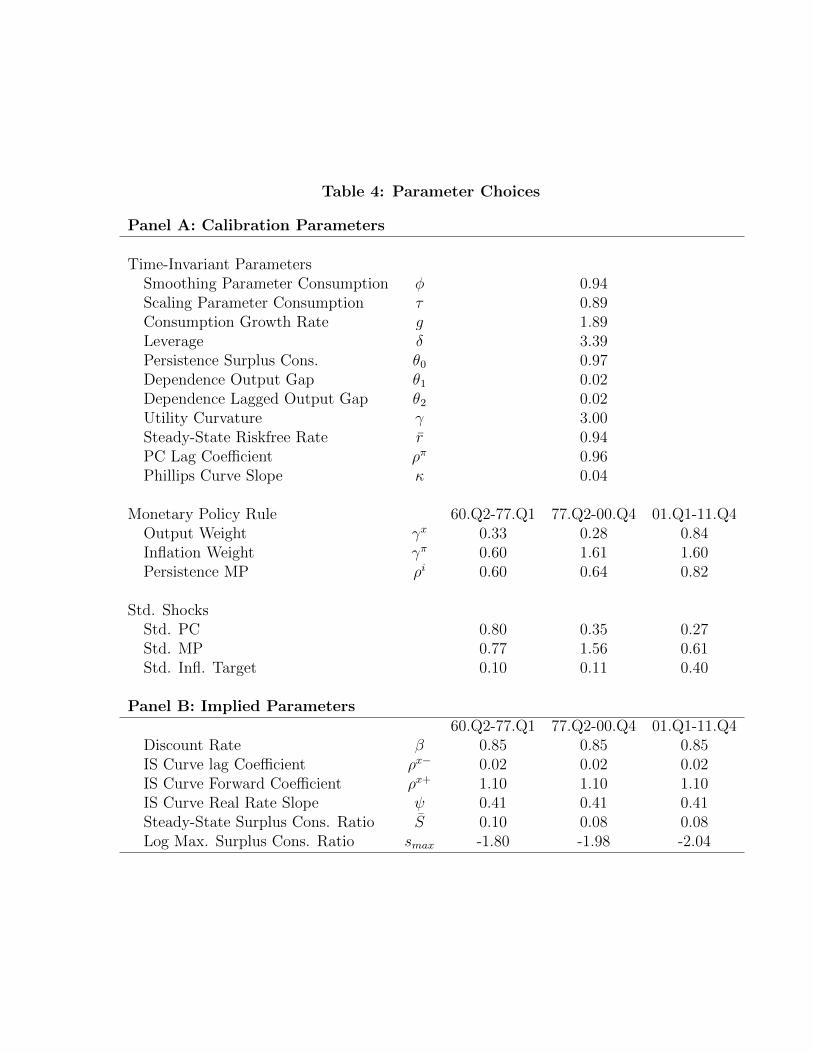
Table 4: Parameter Choices

Panel A: Calibration Parameters

Time-Invariant ParametersSmoothing Parameter Consumption φ 0.94Scaling Parameter Consumption τ 0.89Consumption Growth Rate g 1.89Leverage δ 3.39Persistence Surplus Cons. θ0 0.97Dependence Output Gap θ1 0.02Dependence Lagged Output Gap θ2 0.02Utility Curvature γ 3.00Steady-State Riskfree Rate r 0.94PC Lag Coefficient ρπ 0.96Phillips Curve Slope κ 0.04

Monetary Policy Rule 60.Q2-77.Q1 77.Q2-00.Q4 01.Q1-11.Q4Output Weight γx 0.33 0.28 0.84Inflation Weight γπ 0.60 1.61 1.60Persistence MP ρi 0.60 0.64 0.82

Std. ShocksStd. PC 0.80 0.35 0.27Std. MP 0.77 1.56 0.61Std. Infl. Target 0.10 0.11 0.40

Panel B: Implied Parameters60.Q2-77.Q1 77.Q2-00.Q4 01.Q1-11.Q4

Discount Rate β 0.85 0.85 0.85IS Curve lag Coefficient ρx− 0.02 0.02 0.02IS Curve Forward Coefficient ρx+ 1.10 1.10 1.10IS Curve Real Rate Slope ψ 0.41 0.41 0.41Steady-State Surplus Cons. Ratio S 0.10 0.08 0.08Log Max. Surplus Cons. Ratio smax -1.80 -1.98 -2.04

Table 5: Model and Empirical Moments

Panel A: Estimated MP Rule – Fed Funds onto Output Gap, Infl. and Lag. Fed Funds

60.Q2-77.Q1 77.Q2-00.Q4 01.Q1-11.Q4Empirical Model Empirical Model Empirical Model

Output Gap 0.17** 0.15 0.03 -0.10 0.04 0.06Inflation 0.21** 0.29 0.41* 0.36 0.21** 0.16Lagged Fed Funds 0.69** 0.71 0.66* 0.63 0.83** 0.84

Panel B: Subperiod Second Moments

60.Q2-77.Q1 77.Q2-00.Q4 01.Q1-11.Q4Std. Asset Returns Empirical Model Empirical Model Empirical Model

Std. Eq. Ret. 18.35 16.19 15.68 16.49 20.34 15.48Std. Nom. Bond Ret. 4.92 1.38 8.11 2.65 5.92 3.58Nominal Bond Beta 0.07** 0.05 0.12 0.12 -0.18** -0.16Std. Real Bond Ret. 5.06 2.13 4.27 2.20Real Bond Beta -0.29 0.05 -0.08 -0.07

Std. VAR(1) ResidualsOutput Gap 0.83 1.23 0.76 1.05 0.67 0.96Inflation 1.05 0.78 1.04 0.32 0.86 0.26Fed Funds Rate 0.90 0.75 1.55 1.51 0.47 0.58Log Nominal Yield 0.47 0.14 0.77 0.27 0.56 0.38

This table reports average model moments from 2 simulations of length 50000. * and ** denote significance at the 5% and 1%levels. We use Newey-West standard errors with 2 lags for the nominal bond beta and Newey-West standard errors with 6 lagsfor the empirical Taylor rule estimation.

Table 6: Consumption and Risk Premia

Consumption and Output Gap Empirical ModelStd. Cons. Innovation 1.53 1.94AR(1) Coefficient Output Gap 0.96 0.92Twelve Quarter Cons. Variance Ratio 0.95

EquitiesEquity Premium 4.50 8.37Price-Dividend Ratio (exp(mean(p-d)) 30.05 34.85Std(d-p) 0.40 0.21AR(4) Coefficient d-p 0.92 0.89Correlation(x,p-d) 0.54 0.80Slope 1 YR Exc. Stock ret. wrt d-p 0.08 0.19Slope 5 YR Exc. Stock ret. wrt d-p 0.25 0.73Slope quarterly stock ret. wrt x -0.49 -0.32Slope quarterly annualized std. stock ret. wrt x -1.03 -0.61

Nominal 5-Year Zero Coupon BondNominal Bond Excess Return 1.60 0.23Slope Term Structure 1.06 0.28Subperiod Average Bond Excess Return onto Term Spread 2.88 2.14Correlation(Fed Funds, Slope Term Structure) -0.44 -0.59Std(real rate) (Percent, Ann.) 1.83

The model consumption and output gap dynamics are computed analytically. All othermodel moments are simulated as described in Table 5. Model moments report weightedaverages across subperiods, where weights are proportional to the length of the empiricalperiod. Empirical moments are for the full sample. We proxy for the quarterly annualizedstandard deviation of stock returns with two times the absolute one-quarter stock return inpercent. The subperiod average bond excess return onto the term spread is compared to aquarterly Campbell and Shiller (1991) regression for the full sample.

Table 7: Risk Premium Decomposition

Nominal 5-Year Bond-Stock Correlation 60.Q2-77.Q1 77.Q2-00.Q4 01.Q1-11.Q4Risk Neutral 0.41 0.70 -0.57Risk Premium 0.83 0.79 -0.77Combined 0.54 0.75 -0.71

Real 5-Year Bond-Stock CorrelationRisk Neutral -0.84 0.41 -0.28Risk Premium -0.77 0.43 -0.30Combined -0.93 0.41 -0.50

Combined returns are the sum of risk-neutral and risk premium components. We computerisk neutral nominal and real bond returns as innovations to expected interest rates (Camp-bell and Ammer 1993). The risk premium component of nominal and real bond returnscorresponds to innovations in expected excess returns. Risk neutral stock returns are thesum of innovations to dividends and real interest rates in a Campbell and Shiller (1988)approximate loglinear decomposition. The risk premium component corresponds to innova-tions in expected excess returns. The loglinearization constant is chosen to match simulatedsubperiod average equity price-dividend ratios for combined equity returns for each subpe-riod.

Figure 1: US Nominal Bond Beta, Bond Volatility, and Monetary Policy BreakDates

Nominal bond beta and standard deviation of nominal bond returns from daily bond andstock returns over past three months. The unconditional mean is shown with a red horizontalline. We model time-varying second moments as an unobserved trend AR(1) component pluswhite measurement noise. We show trend second moments estimated using the Kalman filter.95% confidence intervals, which do not take into account parameter uncertainty, are shownin dashed. Gray vertical lines depict Hamilton (2009) oil price shocks.

Figure 2: US Output Gap, Detrended Consumption, and Equity Price-DividendRatio

Panel A: Output Gap and Detrended Consumption

510

1520

Exp

. Det

rend

ed C

ons.

(%

)

-10

-50

510

Log

Out

put G

ap (

%)

60 70 80 90 00 10Year

Log Output Gap (%) Exp. Detrended Cons. (%)

Panel B: Output Gap and Price-Dividend Ratio

2.5

33.

54

4.5

Log

Pric

e-D

ivid

end

Rat

io

-10

-50

510

Log

Out

put G

ap (

%)

60 70 80 90 00 10Year

Log Output Gap (%) Log Price-Dividend Ratio

Panel A plots the time series of the US log real output gap together with log real consumptionin excess of its exponential moving average. An annualized smoothing parameter of φ =0.94 corresponds to a half-life of 2.6 years. We use real consumption expenditures datafor nondurables and services from the Bureau of Economic Analysis National Income andProduct Accounts Tables. The US log output gap (%) is described in Table 1. The end-of-quarter price dividend ratio is computed as the S&P 500 real price divided by real dividendsaveraged over the past 10 years.

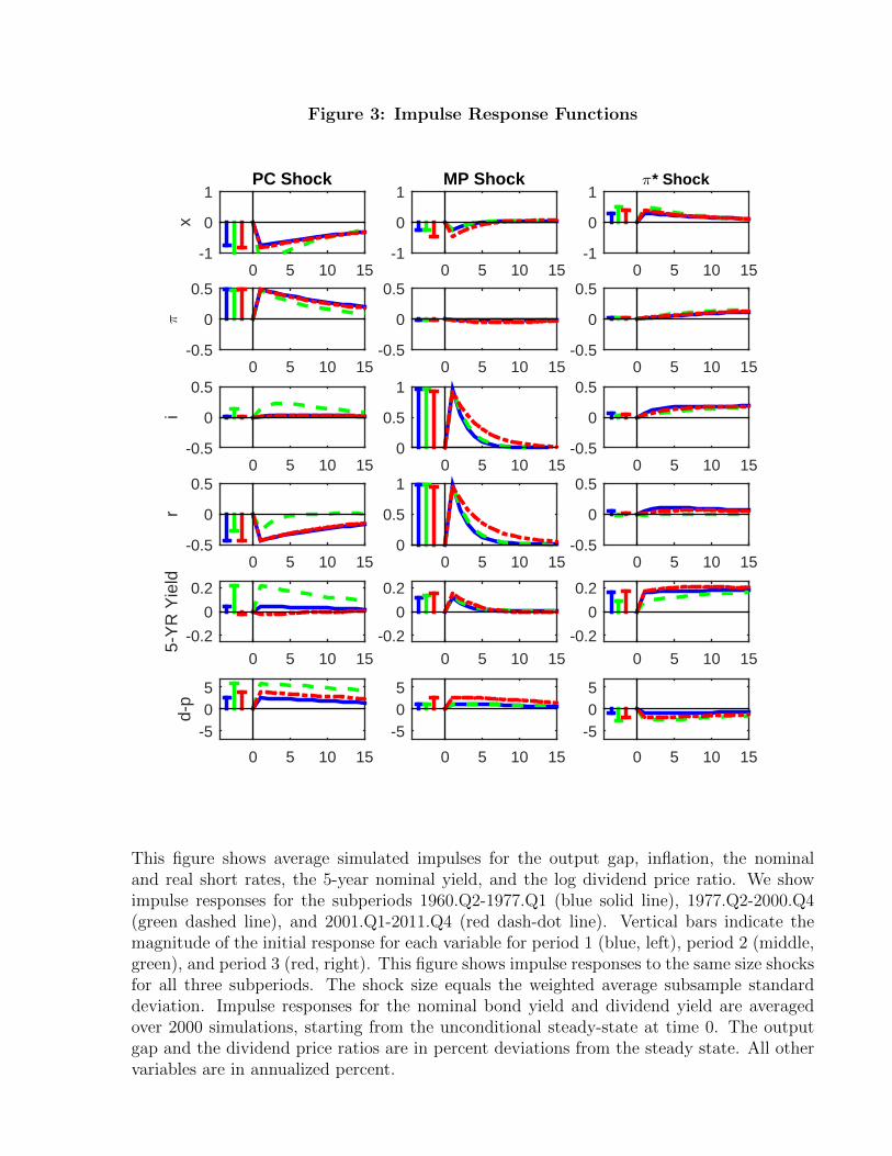
Figure 3: Impulse Response Functions

0 5 10 15

x

-1

0

1PC Shock

0 5 10 15-1

0

1MP Shock

0 5 10 15-1

0

1:* Shock

0 5 10 15

:

-0.5

0

0.5

0 5 10 15-0.5

0

0.5

0 5 10 15-0.5

0

0.5

0 5 10 15

i

-0.5

0

0.5

0 5 10 150

0.5

1

0 5 10 15-0.5

0

0.5

0 5 10 15

r

-0.5

0

0.5

0 5 10 150

0.5

1

0 5 10 15-0.5

0

0.5

0 5 10 15

5-Y

R Y

ield

-0.2

0

0.2

0 5 10 15

-0.2

0

0.2

0 5 10 15

-0.2

0

0.2

0 5 10 15

d-p

-505

0 5 10 15

-505

0 5 10 15

-505

This figure shows average simulated impulses for the output gap, inflation, the nominaland real short rates, the 5-year nominal yield, and the log dividend price ratio. We showimpulse responses for the subperiods 1960.Q2-1977.Q1 (blue solid line), 1977.Q2-2000.Q4(green dashed line), and 2001.Q1-2011.Q4 (red dash-dot line). Vertical bars indicate themagnitude of the initial response for each variable for period 1 (blue, left), period 2 (middle,green), and period 3 (red, right). This figure shows impulse responses to the same size shocksfor all three subperiods. The shock size equals the weighted average subsample standarddeviation. Impulse responses for the nominal bond yield and dividend yield are averagedover 2000 simulations, starting from the unconditional steady-state at time 0. The outputgap and the dividend price ratios are in percent deviations from the steady state. All othervariables are in annualized percent.

Figure 4: Risk Neutral and Risk Premium Impulse Responses

0 5 10 15

dp N

eutr

al

-5

0

5

PC Shock

0 5 10 15

-5

0

5

MP Shock

0 5 10 15

-5

0

5

: * Shock

0 5 10 15

dp P

rem

ium

-5

0

5

0 5 10 15

-5

0

5

0 5 10 15

-5

0

5

0 5 10 15

Yie

ld N

eutr

al

-0.2

0

0.2

0 5 10 15

-0.2

0

0.2

0 5 10 15

-0.2

0

0.2

0 5 10 15

Yie

ld P

rem

ium

-0.1

0

0.1

0 5 10 15-0.1

0

0.1

0 5 10 15-0.1

0

0.1

This figure shows average simulated impulses for risk neutral and risk premium components of5-year nominal bond yields (‘Yield’) and the log equity dividend-price ratio (‘dp’). Risk neu-tral and risk premium components add up to bond yield and dividend yield responses shownin Figure 3. Risk neutral bond yields are the average of expected future nominal short-terminterest rates. Risk neutral equity dividend yields are from a Campbell and Shiller (1988)approximate loglinear decomposition and correspond to the sum of expected future realshort-term interest rates less expected future dividend growth. We show impulse responsesfor the subperiods 1960.Q2-1977.Q1 (blue solid line), 1977.Q2-2000.Q4 (green dashed line),and 2001.Q1-2011.Q4 (red dash-dot line). Impulse responses are simulated exactly as inFigure 3.

Figure 5: Counterfactual Changes in Nominal and Real Bond Betas

Panel A: Nominal 5-Year Bonds

1970 1980 1990 2000 2010

Mod

el N

omin

al B

ond

Bet

as

-0.25

-0.2

-0.15

-0.1

-0.05

0

0.05

0.1

0.15

0.2

Baseline

Vary MP Rule , <MP, <$ Only

Vary <PC Only

1970 1980 1990 2000 2010

Mod

el N

omin

al B

ond

Bet

as-0.25

-0.2

-0.15

-0.1

-0.05

0

0.05

0.1

0.15

0.2

Vary MP Rule Only

Vary <MP OnlyVary <$ Only

Panel A: Real 5-Year Bonds

1970 1980 1990 2000 2010

Mod

el R

eal B

ond

Bet

as

-0.5

-0.4

-0.3

-0.2

-0.1

0

0.1

Baseline

Vary MP Rule , <MP, <$ Only

Vary <PC Only

1970 1980 1990 2000 2010

Mod

el R

eal B

ond

Bet

as

-0.5

-0.4

-0.3

-0.2

-0.1

0

0.1

Vary MP Rule Only

Vary <MP OnlyVary <$ Only

This figure shows model-implied bond betas for three subperiods. The left panels decomposethe total model-implied bond beta (baseline) into changes in monetary policy and changesin PC shock volatilities. The right panels decompose changes in bond betas due to mon-etary policy into different monetary policy components. All parameters not listed in thecorresponding legend are held constant at their period 1 values.