No 133- June 2011

Monetary Policy Transmission, House Prices and Consumer Spending in South Africa: An

SVAR Approach

Mthuli Ncube and Eliphas Ndou

Correct citation: Ncube, Mthuli and Ndou, Eliphas (2011), Monetary Policy Transmission, HousePrices and Consumer Spending in South Africa: An SVAR Approach, Working Paper Series N° 133,African Development Bank, Tunis, Tunisia.

Vencatachellum, Désiré (Chair) Anyanwu, John C. Verdier-Chouchane, Audrey Ngaruko, Floribert Faye, Issa Shimeles, Abebe Salami, Adeleke

Coordinator

Working Papers are available online at http:/www.afdb.org/

Copyright © 2011 African Development Bank Angle des l’avenue du Ghana et des rues Pierre de Coubertin et Hédi Nouira BP 323 -1002 TUNIS Belvédère (Tunisia) Tél: +216 71 333 511 Fax: +216 71 351 933 E-mail: afdb@afdb.org

Salami, Adeleke

Editorial Committee Rights and Permissions

All rights reserved.

The text and data in this publication may be reproduced as long as the source is cited. Reproduction for commercial purposes is forbidden.

The Working Paper Series (WPS) is produced by the Development Research Department of the African Development Bank. The WPS disseminates the findings of work in progress, preliminary research results, and development experience and lessons, to encourage the exchange of ideas and innovative thinking among researchers, development practitioners, policy makers, and donors. The findings, interpretations, and conclusions expressed in the Bank’s WPS are entirely those of the author(s) and do not necessarily represent the view of the African Development Bank, its Board of Directors, or the countries they represent.

Monetary Policy Transmission, House Prices and Consumer Spending in South Africa: An SVAR Approach

Mthuli Ncube and Eliphas Ndou(1)

___________

AFRICAN DEVELOPMENT BANK GROUP

Working Paper No. 133

June 2011

(1) Mthuli Ncube and Eliphas Ndou are respectively Chief Economist and Vice President of the African Development Bank, Tunis, Tunisia (M.Ncube@afdb.org) and Researcher at the South African Reserve Bank, Research Department, Pretoria, South Africa.

Office of the Chief Economist

1. Introduction This paper aims to estimate and quantify the percentage decline in consumption expenditure, which can be attributed to changes in house wealth, after monetary policy tightening. We use the structural vector autoregressive (SVAR) approach on South African disaggregated Absa house price data, namely all-size, large-size and medium-size and small-size house prices. There are two channels through which interest rate changes can affect consumption, namely the direct and indirect effects (HM Treasury (2003). The direct link suggests that changes in interest rates affect consumption directly. The indirect effects operate in two stages. Firstly, changes in interest rates will impact on housing demand and supply which will consequently lead to changes in house prices and house wealth. Secondly, declines in housing wealth directly reduce current consumption. The direct effect suggests that increases in interest rates have an income or cash-flow effect. Any interest rate rises increase the burden of mortgage interest payments which directly reduce current consumption. This implies that changes in interest rates can, to some extent, in the short term, reduce current consumption through altering the after-mortgage payments household disposable income available for current spending. HM treasury (2003) suggests that the direct effects of interest rates on consumer spending are stronger when individual households have net exposure on interest-bearing debt, a large proportion of contracts use variable interest rates, when consumers are credit constrained and when the link between base rate and mortgage rate is strong. Both ways of transmission of interest rates to consumer spending predict housing prices and consumption are inversely related to the prevailing level of interest rate. Elbourne (2008), using an eight-variable SVAR approach, deduced that in the United Kingdom (UK) about 15 percent of the decline in consumption following an interest rate shock could be explained by a combined effect of house wealth and credit effects associated with house price changes. Lacoviello (2002) found that house prices fell by 1,5 percent after a 50 basis point interest shock. He concluded that monetary policy had a significant effect on house prices. Lacoviello and Minnetti (2007) tested the credit channel of monetary policy in the housing market using the VAR method for different housing markets (i.e., Finland, Germany, Norway and UK). They found that house prices fell by nearly 1 percent after a 70 basis point interbank interest rate shock depending on the method of estimation used and indicated as evidence of a bank lending channel and maybe a balance-sheet channel. Case et al. (2005) estimated various regressions relating consumption to income and wealth measure for 14 European countries. They found that a 10 percent rise in house prices increased consumption by 1 percent for a panel of western countries. Evidence in Lacoviello (2004) from the Euler equation for consumption in the United States (US) showed that changes in house prices had significant effects on consumption There are some studies in South Africa which discussed the impact of monetary policy on disaggregated house prices inflation. Gupta and Kabundi (2010) used a factor augmented vector autoregressive (FAVAR) and found that house price inflation was negatively related to monetary policy shocks in South Africa. Kasai

5

and Gupta (2010), using an SVAR found that during the period of financial liberalisation interest rate shocks had relatively stronger effects on house price inflation irrespective of house sizes in South Africa. However, these South African studies did not quantify the indirect effects of interest rate changes working through changes in house prices on consumer spending. We fill the gap by estimating and quantifying the role of house wealth in South Africa using disaggregated house prices. In addition, there has been little, if any, empirical discussion of the wealth effects of gains in the housing market in South Africa.1 We estimated an SVAR model based on the Elbourne (2008) model using disaggregated South African Absa house price data in the period 1975Q1 to 2009Q4. The SVAR approach has advantages over the recursive identification approach. Jacobs et al. (2003) suggest that SVARs can be used to analyse short-run dynamics and the speed towards equilibrium, and indicate the sources of shocks. Gottschalk (2001) argues that SVAR approaches are useful for taking a theory-guided look at data; restrictions are compatible with a large number of theories, which allows the use of the SVAR methodology to discriminate between competing theories. We argue that when house prices are influenced by interest rate and consumption depends on housing wealth there is a channel of monetary policy transmission through house prices. This paper assesses the overall importance of housing wealth and housing market-related credit imperfections in the South African monetary transmission mechanism to real spending. The results at the peak of interest rate effects on consumption suggest that consumption declines due to the combined effect of house wealth and credit changes following a monetary policy tightening by 9,8 percent in all-size, 3,7 percent in small-size, 4,7 percent in medium-size and 5,3 percent in large-size houses. The findings indicate the heterogeneity in the transmission of interest rate effects operating through house wealth and credit channel. Moreover, we reached the same conclusion after modifying the baseline model by adding the restrictions that house price also respond to both aggregate demand and aggregate supply variables. Lastly, the differences between the counterfactual consumption and baseline consumption responses provide little support that the house wealth channel is the dominant source of monetary policy transmission to consumption. The rest of the paper is organised such that Section 2 describes monetary policy transmission and house prices and related the literature. The SVAR modelling approach is presented in Section 3 and data description in Section 4. Section 5 presents and explains the results and Section 6 gives the conclusions. 1 We could not get the figures indicating the extent of mortgage equity withdrawals in South Africa and hope this study will stimulate relevant data collection.

6

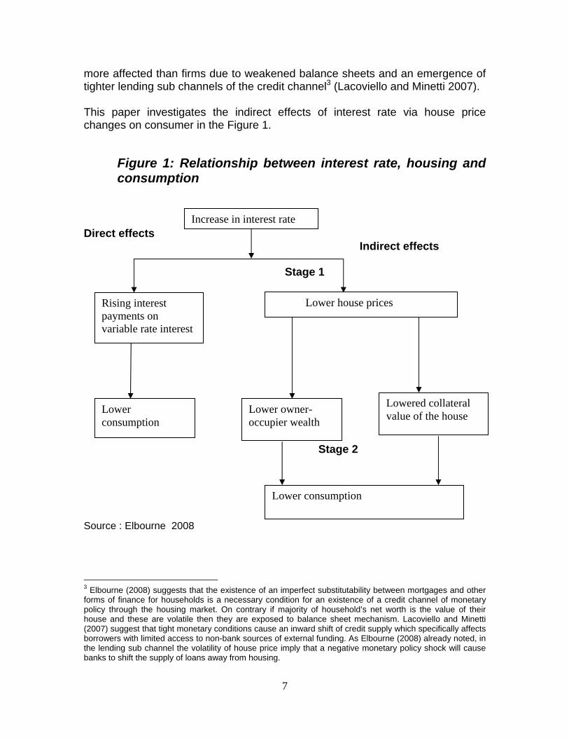
2. Consumption, housing prices and interest rates The level of household consumption spending depends on house wealth which also changes with house prices and real interest rates. Monetary policy decisions, which change short-term interest rates, affect the housing market and the whole economy, both directly and indirectly through a number of channels. The direct effects of interest rates work through the costs of capital, expectations of house price movements and house supply. The indirect effects work via the wealth effect from house price changes, and balance-sheet effects through the credit channel on both consumer spending and housing demand. The direct and indirect effects of monetary policy transmission are shown in Figure 1 adopted from the Elbourne (2008). The direct effect occurs through the income or cash-flow effect, in which a higher interest rate increases the burden of any outstanding variable interest debt payments. Any debt interest payments increase leads to reduced cash flow and a decrease in after-housing costs disposable income, prompting households’ expenditure declines in the shorter term. The cash-flow effects are greater the closer the household are nearer to wiping out their budgets, and the more constrained households to access credit, and the more responsiveness the variable or fixed rates to changes in base rates set by central bank. These indirect effects in Figure 1 operate through wealth effects and credit channel effects (Elbourne 2008). The indirect effects of an interest rate hike operate in two stages. Firstly, asset-pricing theory suggests an inverse relationship between interest rates and house prices. Secondly, falling house prices reduce owner-occupier wealth and cash flow, and lower the collateral value of the house.2 These deteriorations limit households’ access to credit. Credit constrained consumers who use house collateral when borrowing will cut consumption in response to declining house prices. Wealth effects occur when an increase in house prices gives individuals more assets to spend throughout their lifetimes. Based on the life-cycle hypothesis, consumers should increase their consumption due to increased wealth. Lacoviello and Minetti (2007) argue that house prices play an important role in the transmission of monetary policy through credit-supply shifts and through determination of the lender’s net worth, which constrain the amount of credit made available. Households that depend on credit find that higher interest rates reduce their household wealth, and lower the chances of household access to credit by decreasing house collateral value. The credit channel of monetary transmission suggests that credit-constrained households are more likely to reduce their consumption spending following a decline in house prices (Elbourne 2008). Moreover, households are likely to be

2 The reduced cash flows reduces size of mortgage which the credit-constrained household can afford or qualify for, hence lowering the value of house they can purchase (Miskin 2007).

7

more affected than firms due to weakened balance sheets and an emergence of tighter lending sub channels of the credit channel3 (Lacoviello and Minetti 2007). This paper investigates the indirect effects of interest rate via house price changes on consumer in the Figure 1.

Figure 1: Relationship between interest rate, housing and consumption

Direct effects Indirect effects Stage 1

Stage 2 Source : Elbourne 2008

3 Elbourne (2008) suggests that the existence of an imperfect substitutability between mortgages and other forms of finance for households is a necessary condition for an existence of a credit channel of monetary policy through the housing market. On contrary if majority of household’s net worth is the value of their house and these are volatile then they are exposed to balance sheet mechanism. Lacoviello and Minetti (2007) suggest that tight monetary conditions cause an inward shift of credit supply which specifically affects borrowers with limited access to non-bank sources of external funding. As Elbourne (2008) already noted, in the lending sub channel the volatility of house price imply that a negative monetary policy shock will cause banks to shift the supply of loans away from housing.

Increase in interest rate

Rising interest payments on variable rate interest

t

Lower house prices

Lower owner-occupier wealth

Lower consumption

Lowered collateral value of the house

Lower consumption

8

2.2. The effect of monetary policy on house prices The demand for houses is negatively related to interest rates because interest rate payments represent a major portion of the house purchase decisions (Elbourne 2008). According to Maclennan et al. (2000) interest rates represent the overall costs of investing in the house relative to other assets. Therefore, house prices are sensitive to the investment return on other financial assets, such as bonds. The substitution effect of an interest rate increase causes a portfolio switch by households into less liquid assets. Thus, there is a shift away from non-interest rate-bearing bank deposits into interest rate-bearing deposits (Maclennan et al 2000).4 In addition, households that experience a decrease in house wealth due to higher interest rates may lower their consumption expenditure due to capital losses.5 High interest rates are relevant at the beginning of a new interest rate payment period through impacting on interest payments on new housing loans. Hence, the amount an individual is willing to pay will be directly linked to the affordability of initial interest rate payments. Alternatively, higher interest rates lower house prices by increasing the burden of variable interest rate to such an extent that houses need to be sold to pay back the principal or the house is repossessed (Elbourne 2008). The speed at which house prices constrain consumption, after a monetary policy contraction, depends on the rate of adjustment of mortgage interest rate, mortgage structure and interest rate period. Calza, Moacelli, and Stracca (2006) found that sensitivity of consumer spending to monetary policy shocks increases with the lowering of the down payment and lowering of the mortgage repayment rate, and become larger under a variable rate mortgage structure. The correlation between consumption and house prices increases with the degree of flexibility or development of mortgage markets. The shorter the duration of interest rates the faster these changes will affect household disposable income (Elbourne 2008). Moreover, the more variable rates respond to official interest rates, the greater the probability that spending will react quickly to changes in interest rates. Alternatively, the shorter the interest rate period of the loan, the stronger the interest rate impact on mortgage rates. HM treasury (2003) suggested that the direct effects on consumption are strongest where the level of interest rate-bearing debt is high in relation to interest bearing assets, strong link between base and mortgage rates, and when consumers are credit constrained. Aoki et al. (2002) used VAR methods to examine the responsiveness of UK house prices to 50 basis points short-term interest rate increase and concluded that a peak decline of house prices occurred after five quarters at 0,8 percent and durable goods declined by 0,8 percent which is larger than 0,1 percent for

4 Maclennan et al (2000) argues that the magnitude and timing of these portfolio-switching effects is debatable. He cites that a rise in interest rate may induce households to become more cautious hence in turn save more in liquid forms and hold off from buying bonds and equities in cases their prices should fall further down 5 HM Treasury (2003) takes a cautionary approach that exploitation of capital gains depends on the degree households wealth can be liquidated, and behaviour of lending institutions.

9

non-durable goods. Lacoviello (2002) estimated structural VARs model for six European countries using the identification scheme of King et al. (1991). Evidence found based on quarterly data over the period 1973Q1 to 1998Q3 for the UK revealed that house prices fell by 1,5 percent after normalising interest to represent a 50 basis point interest shock. Lacoviello and Minnetti (2007) tested the credit channel of monetary policy in the housing market using the VAR method and identification, as in King et al (1991). Three different vector error-correction models and VAR for each of the four different housing markets, namely Finland, Germany, Norway and UK were estimated using quarterly data over the period 1978Q4 to 1994Q4. House prices fell by about 0,7–1 percent after a 70 basis point interbank interest rate shock with the bank lending channel and maybe a balance-sheet channel. Giuliodori (2005) estimated a number of VAR models separately for nine countries using the recursive ordering over the period 1979Q1 to 1998Q4 and found that real house prices fell by 0,7 percent or 1,8 percent after a 100 basis point money-market shock depending on the model used. The study showed that house prices might enhance the effects of a monetary policy shock on consumer spending in those economies where housing and mortgage markets are relatively developed and competitive. Gupta and Kabundi (2010) assessed the impact of monetary policy on real house price growth in South Africa, using a factor augmented vector autoregressive (FAVAR) over the period 1980Q1 to 2006Q4. Results from their impulse response function indicated, in general, that house price inflation was negatively related to monetary policy shocks but the effects were transmitted heterogeneously across housing segments. Kasai and Gupta (2010) investigated the effectiveness of monetary policy on house prices in South Africa before and after financial liberalisation. They found that during the period of financial liberalisation, interest rate shocks had relatively stronger effects on house price inflation irrespective of house sizes. These South African studies focused on assessing the direct relationship between an interest rate increase and house price inflation. This paper aims to estimate and quantify the percentage declines in real consumption expenditure, which can be attributed to combined house wealth and credits effects due to interest rate changes. 2.3. The effects of house prices on consumption According to Elbourne (2008) it is important to show an indirect housing market channel of monetary policy working through house prices which affect consumption. We note that not all house wealth related to house prices can be consumed. Institutional differences which lower real house price volatility tend to lessen sensitivity of house prices to consumption, and weaken the role of real house prices in the interest rate transmission mechanism (Maclennan et al.,

10

2000). Factors such as high transaction costs, a low loan-to-value ratio, lower the level of the owner-occupier sector, a larger proportion of households in the private-rented sector and a large proportion of fixed interest mortgage loans weaken the sensitivity of consumption to house price changes. It is noted in Elbourne (2008) that low transaction costs make housing more liquid. Rising house prices have negative effects for the rented sector (Maclennan et al., 2000, Elbourne 2008). Rent payers expect to pay higher future rental rates and a large down payment when purchasing a house. With wealth effects being smaller for institutional investors owning rental housing than owner occupiers, all else equal, the higher proportion of owner occupier and the lower proportion of households in the market-rented sector make the response of consumption to increase in house prices larger. Households can use housing wealth gains to fund their current consumption.6 Case et al. (2005) estimated various regressions relating consumption to income and wealth measure for 14 countries, and concluded that the effect of the housing market on consumption was significant relative to the stock market. Quantitatively they found that an immediate effect of a 10 percent increase in house wealth resulted in consumption rising by 1 percent for a panel of Western countries. Evidence in Lacoviello (2004) from Euler equation for consumption in US showed that changes in house prices had significant effects on consumption. Chirinko et al. (2004) estimated an SVAR for 13 countries with non-recursive contemporaneous restrictions on data over the period 1979Q4 to 1998Q4. The cumulative rise of UK consumption reached about 0,7 percent over one year, after a 1 percent shock to house prices. They showed that house price shocks have bigger effects than equity. Elbourne (2008) argues that to establish the existence of an indirect housing market channel of monetary policy, one needs to show that not only monetary policy affects house prices but changes in house prices affect consumption. Using a structural VAR based on monthly data from January 1987 to May 2003, Elbourne inferred that about 15 percent of a fall in consumption is due to a combined effect of house wealth and credits effects from monetary policy tightening. He concludes from impulse response evidence that housing wealth indeed plays a role but not as large as suggested by the Guillidori (2005) estimates from recursive Cholesky decomposition approach. 2.4 Evidence from counterfactual studies Counterfactual simulation approaches were also used to show the importance of the wealth channel in consumer spending. Giuliodori (2005) found significant

6 In Elbourne (2008) evidence suggests the positive effect of increases in house prices on consumption. Maclennan et al (2000) suggests; where housing was regarded as excellent collateral; housing is in effect more spendable and house prices impact much stronger on consumer spending.

11

consumption increase following a real house price shock using a VAR. The importance of real house prices in the transmission mechanism was measured by simulating a model in which consumption does not respond directly to house prices by making the coefficients of contemporaneous and lagged house prices in the consumption equation to zero. Evidence indicated that peak consumption response to a monetary contraction is about 0,5 per cent in the unrestricted setting but only about 0,2 percent in the restricted model. Elbourne (2008) used an SVAR approach to infer that about 15 percent of the fall in consumption was due to the combined role of the housing wealth effect channel and housing credit channel. However, the counterfactual approach attributes about 12 percent of consumption fall to combined wealth and credit effects. Moreover the impulse responses from the counterfactual model were similar to those under the baseline scenarios being within the error bands of the baseline model. Ludvigson and Lettau (2002) estimated five-variable and six-variable SVAR models for non-durable and services, as well as total personnel consumption expenditure. In both forms of VARs, the total personnel consumption expenditure and its non-durable consumption component were found to be virtually identical under the baseline and counterfactual scenarios. They concluded that the wealth channel was relatively an unimportant one in transmitting the effects of monetary policy to consumer sector. Aoki et al. (2004) developed and calibrated the dynamic general stochastic equilibrium model with frictions in the credit markets used by households. The results revealed big differences between the impulse responses with and without a financial accelerator in response to a 50 basis point monetary policy shock. After switching on the financial accelerator channel in the model, the impulse responses of consumption and house price increased much in line with the results from the VAR evidence.

12

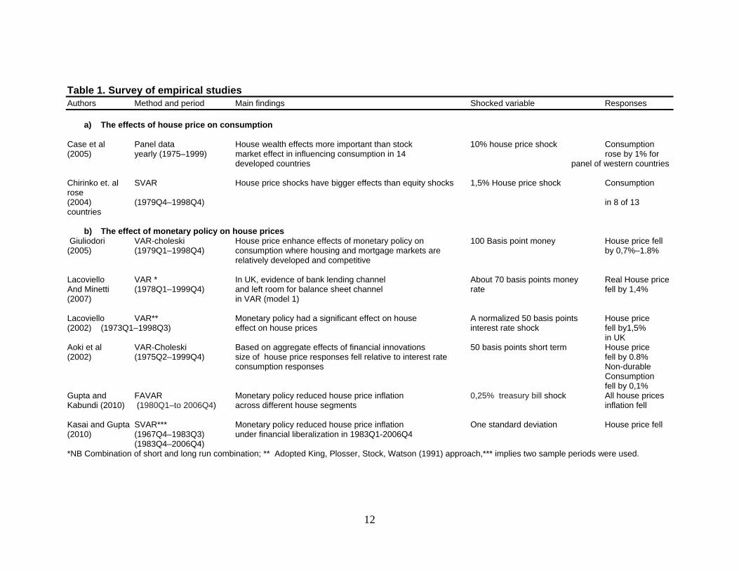
Table 1. Survey of empirical studies Authors Method and period Main findings Shocked variable Responses

a) The effects of house price on consumption Case et al Panel data House wealth effects more important than stock 10% house price shock Consumption (2005) yearly (1975–1999) market effect in influencing consumption in 14 rose by 1% for developed countries panel of western countries Chirinko et. al SVAR House price shocks have bigger effects than equity shocks 1,5% House price shock Consumption rose (2004) (1979Q4–1998Q4) in 8 of 13 countries

b) The effect of monetary policy on house prices Giuliodori VAR-choleski House price enhance effects of monetary policy on 100 Basis point money House price fell (2005) (1979Q1–1998Q4) consumption where housing and mortgage markets are by 0,7%–1.8% relatively developed and competitive Lacoviello VAR * In UK, evidence of bank lending channel About 70 basis points money Real House price And Minetti (1978Q1–1999Q4) and left room for balance sheet channel rate fell by 1,4% (2007) in VAR (model 1) Lacoviello VAR** Monetary policy had a significant effect on house A normalized 50 basis points House price (2002) (1973Q1–1998Q3) effect on house prices interest rate shock fell by1,5% in UK Aoki et al VAR-Choleski Based on aggregate effects of financial innovations 50 basis points short term House price (2002) (1975Q2–1999Q4) size of house price responses fell relative to interest rate fell by 0.8% consumption responses Non-durable

Consumption fell by 0,1%

Gupta and FAVAR Monetary policy reduced house price inflation 0,25% treasury bill shock All house prices Kabundi (2010) (1980Q1–to 2006Q4) across different house segments inflation fell Kasai and Gupta SVAR*** Monetary policy reduced house price inflation One standard deviation House price fell (2010) (1967Q4–1983Q3) under financial liberalization in 1983Q1-2006Q4 (1983Q4–2006Q4) *NB Combination of short and long run combination; ** Adopted King, Plosser, Stock, Watson (1991) approach,*** implies two sample periods were used.

13

Table 1 continued

b.1) Combined role of housing wealth- and housing credit channel Elbourne SVAR House price explain about one-seventh of 100 basis point s interest rate house price (2008) (198M1-2003M5) fall in consumption after interest rate hike shock fell by 0,75%. Retail sales fell by 0,4%

c) Counterfactual studies Elbourne SVAR 12% of consumption decline- attributed to falling house 100 basis point s interest rate house price (2008) (198M1-2003M5) price following interest rate hike fell by 0,75%. Retail sales fell By 0, –4%

Giuliodori VAR-choleski Excluding role of house price, consumption fell from 0.5% 100 Basis point money House price fell (2005) (1979Q3–1998Q4) to 0.2% market interest shock by 0,7%–1,8% Ludvigson and SVAR (5 variables) Absence of wealth channel to consumption had a small One standard deviation Nondurable & andLettau (2001) (1966Q1–2003Q3) impact on the responses of consumption to federal funds rate ( 81 basis point ) services consumption Total PCE was one-tenth of percentage point less at fell by -0.23% its trough when wealth channel is shut off than Total PCE fell under the baseline model by -0,25 to–0,5% Ludvigson and SVAR (6-variables) Wealth channel is relatively unimportant in transmitting the One standard deviation Both nondurable & Lettau (2001) (1966Q1-2003Q3) effects of monetary policy to consumer sector. Very little support (81 basis points) total consumption for view that wealth channel is dominant source of monetary fell by -0,2% transmission to consumption. Both nondurable and total PCE and -0,23% under baseline model virtually not distinguishable from model respectively when wealth channel was shut off. Aoki et al Calibrated DSGE to The DSGE model fitted data when the financial accelerator 50 basis points short term House prices and (2002) VAR (1975Q2-1999Q4) through housing market is switched on interest rate consumption rose under financial accelerator model

14

3. Methodology 3.1 The VAR Model We assume the economy has the structural form equation [1] as in Kim and Roubini (2000) [1] ( ) ttxLA ε= where ( )LA is the matrix polynomial in the lag operator L and tx is an nx1 vector of explanatory variables. tε is nx1 structural disturbance vector which are serial uncorrelated. The residual vector variance is Ω=)var( tε with diagonals as variances of structural disturbances. These structural disturbances are assumed to be mutually uncorrelated. We then estimate the reduced form equation (VAR) [2] ( ) ttt uxLBx += where ( )LB is a matrix polynomial with a constant term in lag operator L and var(ut)= ( )tt uuE ′=∑ .We adopt the structural VAR modelling in which non-recursive structures are allowed while still giving restrictions only on contemporaneous structural parameters. Letting 0A to denote the contemporaneous coefficient matrix in the structural form of non-singular matrix at lag zero in ( )LA and letting ( )LA+ be coefficient matrix in ( )LA at strictly positive lags excluding the contemporaneous coefficient 0A , we express ( )LA as [4] ( ) ( )LAALA ++= 0 . The parameters in the structural form equation and those in the reduced form are related by [5] ( ) ( )LAALB +−−= 0

1 The structural disturbance and the reduced form residuals are related by tt uA0=ε which implies that 0

10

1 −− Ω=∑ AA . According to Kim and Roubini (2000) the maximum likelihood estimates of Ω and 0A are obtained only through sample estimates of ∑ . Since diagonals are

15

normalised to 1`s we need at least 2)1( −× nn restrictions on 0A to over identify

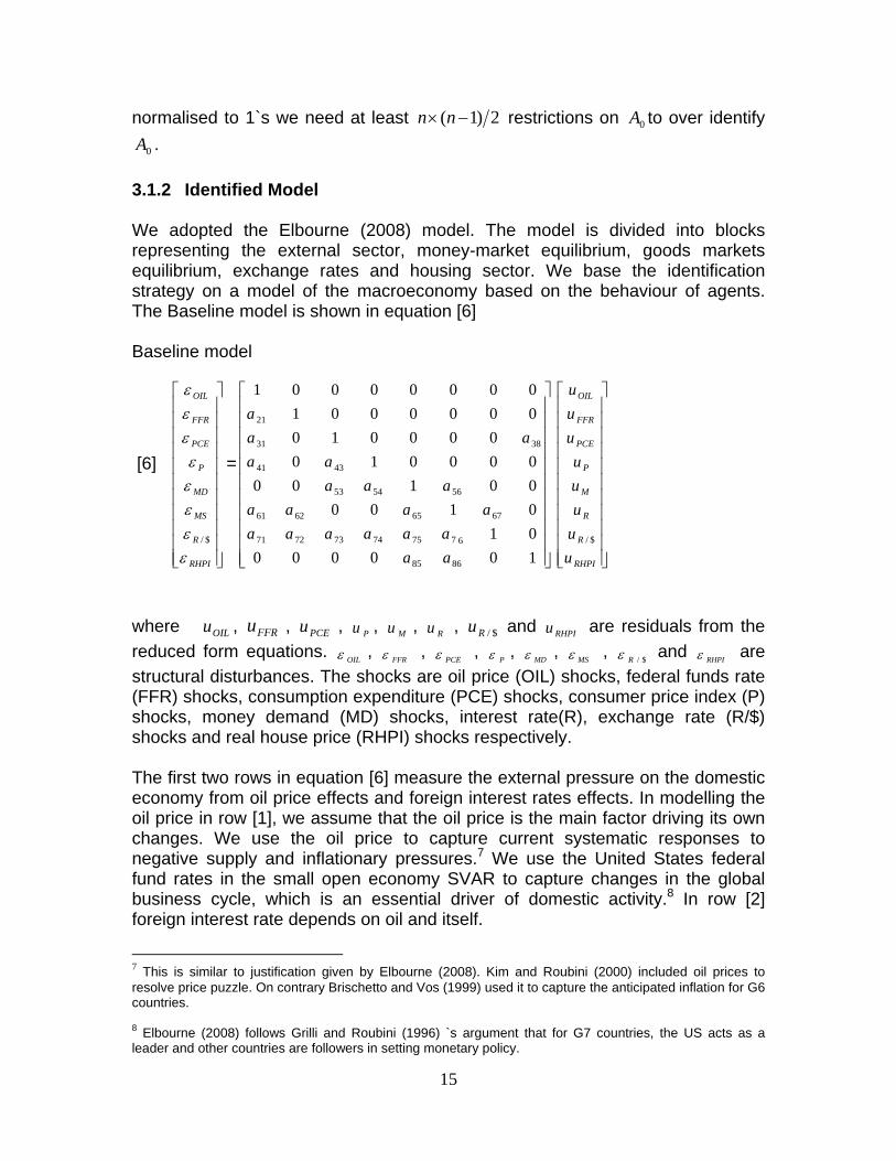
0A . 3.1.2 Identified Model We adopted the Elbourne (2008) model. The model is divided into blocks representing the external sector, money-market equilibrium, goods markets equilibrium, exchange rates and housing sector. We base the identification strategy on a model of the macroeconomy based on the behaviour of agents. The Baseline model is shown in equation [6] Baseline model

[6]

⎥⎥⎥⎥⎥⎥⎥⎥⎥⎥⎥

⎦

⎤

⎢⎢⎢⎢⎢⎢⎢⎢⎢⎢⎢

⎣

⎡

RHPI

R

MS

MD

P

PCE

FFR

OIL

εεεεεεεε

$/

=

⎥⎥⎥⎥⎥⎥⎥⎥⎥⎥⎥

⎦

⎤

⎢⎢⎢⎢⎢⎢⎢⎢⎢⎢⎢

⎣

⎡

10000001010000100000010

000010000000100000001

8685

677574737271

67656261

565453

4341

3831

21

aaaaaaaa

aaaaaaa

aaaa

a

⎥⎥⎥⎥⎥⎥⎥⎥⎥⎥⎥

⎦

⎤

⎢⎢⎢⎢⎢⎢⎢⎢⎢⎢⎢

⎣

⎡

RHPI

R

R

M

P

PCE

FFR

OIL

uuuuu

uuu

$/

where OILu , FFRu , PCEu , Pu , Mu , Ru , $/Ru and RHPIu are residuals from the reduced form equations. OILε , FFRε , PCEε , Pε , MDε , MSε , $/Rε and RHPIε are structural disturbances. The shocks are oil price (OIL) shocks, federal funds rate (FFR) shocks, consumption expenditure (PCE) shocks, consumer price index (P) shocks, money demand (MD) shocks, interest rate(R), exchange rate (R/$) shocks and real house price (RHPI) shocks respectively. The first two rows in equation [6] measure the external pressure on the domestic economy from oil price effects and foreign interest rates effects. In modelling the oil price in row [1], we assume that the oil price is the main factor driving its own changes. We use the oil price to capture current systematic responses to negative supply and inflationary pressures.7 We use the United States federal fund rates in the small open economy SVAR to capture changes in the global business cycle, which is an essential driver of domestic activity.8 In row [2] foreign interest rate depends on oil and itself.

7 This is similar to justification given by Elbourne (2008). Kim and Roubini (2000) included oil prices to resolve price puzzle. On contrary Brischetto and Vos (1999) used it to capture the anticipated inflation for G6 countries. 8 Elbourne (2008) follows Grilli and Roubini (1996) `s argument that for G7 countries, the US acts as a leader and other countries are followers in setting monetary policy.

16

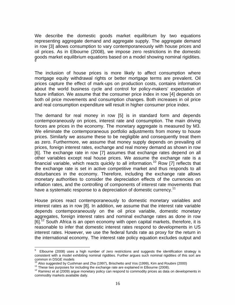
We describe the domestic goods market equilibrium by two equations representing aggregate demand and aggregate supply. The aggregate demand in row [3] allows consumption to vary contemporaneously with house prices and oil prices. As in Elbourne (2008), we impose zero restrictions in the domestic goods market equilibrium equations based on a model showing nominal rigidities. 9 The inclusion of house prices is more likely to affect consumption where mortgage equity withdrawal rights or better mortgage terms are prevalent. Oil prices capture the effect of mark-ups on production costs, contains information about the world business cycle and control for policy-makers’ expectation of future inflation. We assume that the consumer price index in row [4] depends on both oil price movements and consumption changes. Both increases in oil price and real consumption expenditure will result in higher consumer price index. The demand for real money in row [5] is in standard form and depends contemporaneously on prices, interest rate and consumption. The main driving forces are prices in the economy. The monetary aggregate is measured by M3. We eliminate the contemporaneous portfolio adjustments from money to house prices. Similarly we assume these to be negligible and consequently treat them as zero. Furthermore, we assume that money supply depends on prevailing oil prices, foreign interest rates, exchange and real money demand as shown in row [6]. The exchange rate in row [7] assumes that exchange rates depend on all other variables except real house prices. We assume the exchange rate is a financial variable, which reacts quickly to all information.10 Row [7] reflects that the exchange rate is set in active competitive market and thus responds to all disturbances in the economy. Therefore, including the exchange rate allows monetary authorities to consider the depreciation effects of the currencies on inflation rates, and the controlling of components of interest rate movements that have a systematic response to a depreciation of domestic currency.11 House prices react contemporaneously to domestic monetary variables and interest rates as in row [8]. In addition, we assume that the interest rate variable depends contemporaneously on the oil price variable, domestic monetary aggregates, foreign interest rates and nominal exchange rates as done in row [6].12 South Africa is an open economy with open capital markets, therefore, it is reasonable to infer that domestic interest rates respond to developments in US interest rates. However, we use the federal funds rate as proxy for the return in the international economy. The interest rate policy equation excludes output and

9 Elbourne (2008) uses a high number of zero restrictions and suggests the identification strategy is consistent with a model exhibiting nominal rigidities. Further argues such nominal rigidities of this sort are common in DSGE models 10 Also suggested by Cushman and Zha (1997), Brischetto and Vos (1999), Kim and Roubini (2000) 11 These two purposes for including the exchange rate are explained in Elbourne (2008). 12 Ramirez et al (2009) argue monetary policy can respond to commodity prices as data on developments in commodity markets available daily.

17

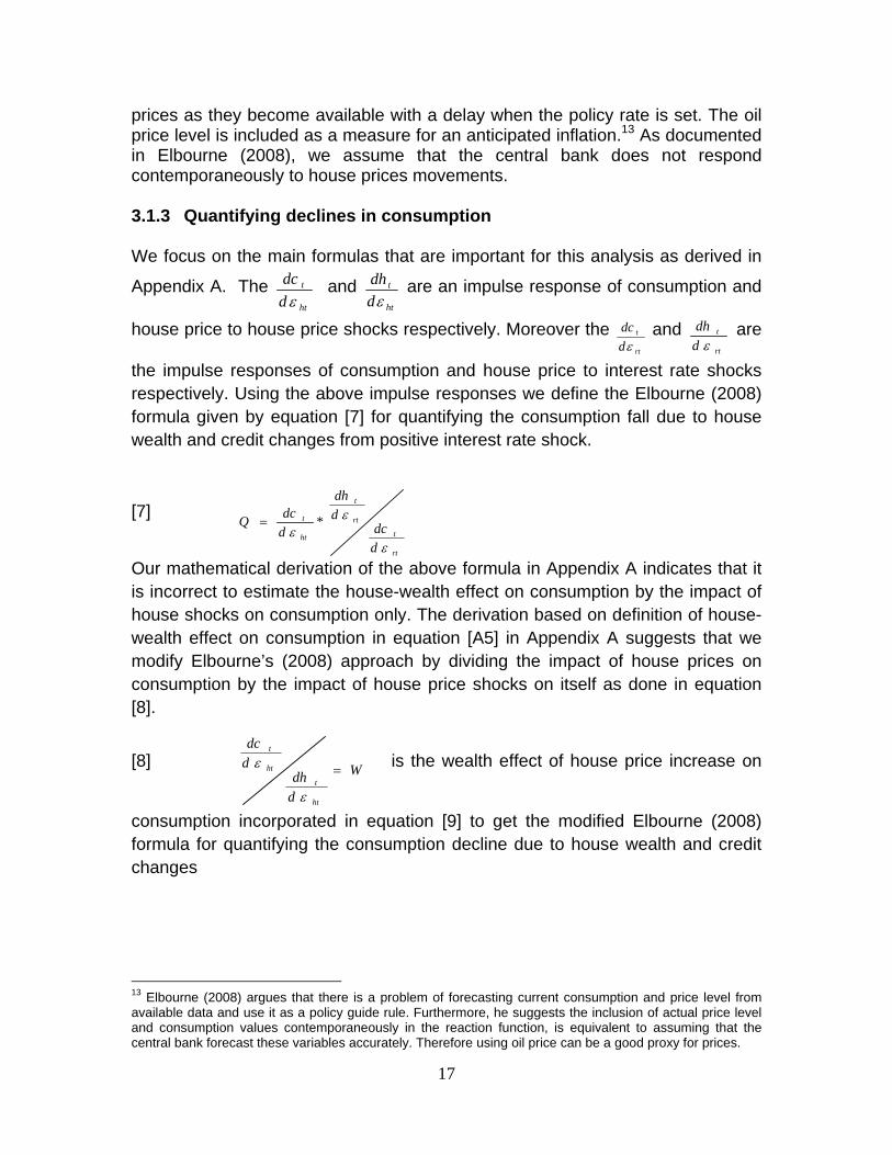
prices as they become available with a delay when the policy rate is set. The oil price level is included as a measure for an anticipated inflation.13 As documented in Elbourne (2008), we assume that the central bank does not respond contemporaneously to house prices movements. 3.1.3 Quantifying declines in consumption We focus on the main formulas that are important for this analysis as derived in

Appendix A. The ht

t

ddcε

and ht

t

ddhε

are an impulse response of consumption and

house price to house price shocks respectively. Moreover the rt

t

ddcε

and rt

t

ddhε

are

the impulse responses of consumption and house price to interest rate shocks respectively. Using the above impulse responses we define the Elbourne (2008) formula given by equation [7] for quantifying the consumption fall due to house wealth and credit changes from positive interest rate shock.

[7]

rt

t

rt

t

ht

t

ddc

ddh

ddcQ

ε

εε

*=

Our mathematical derivation of the above formula in Appendix A indicates that it is incorrect to estimate the house-wealth effect on consumption by the impact of house shocks on consumption only. The derivation based on definition of house-wealth effect on consumption in equation [A5] in Appendix A suggests that we modify Elbourne’s (2008) approach by dividing the impact of house prices on consumption by the impact of house price shocks on itself as done in equation [8].

[8] W

ddh

ddc

ht

t

ht

t

=

ε

ε is the wealth effect of house price increase on

consumption incorporated in equation [9] to get the modified Elbourne (2008) formula for quantifying the consumption decline due to house wealth and credit changes

13 Elbourne (2008) argues that there is a problem of forecasting current consumption and price level from available data and use it as a policy guide rule. Furthermore, he suggests the inclusion of actual price level and consumption values contemporaneously in the reaction function, is equivalent to assuming that the central bank forecast these variables accurately. Therefore using oil price can be a good proxy for prices.

18

[9]

rt

t

rt

t

t

tm

ddc

ddh

WdcdhWQ

ε

ε*== where mQ is.

The paper uses both equations [7] and [9] to quantify the combined wealth and credit effects arising from a change in interest rates increase. 4. Data This paper uses eight variables in the period 1975Q1 to 2009Q4 to examine the transmission of monetary policy in real house prices and consumer spending in South Africa. Domestic variables are consumer price variable, consumption expenditure,14 money-market interest rate, money supply, real house price; nominal exchange rate and oil index (average Brent crude). We deflate house prices by the consumer price to make them real. The consumption expenditure data come from the South African Reserve Bank. We use the Federal fund rate as a foreign variable to capture the foreign interest rate influence on South Africa open economy. The money-market interest rate represents the monetary policy stance. These variables were extracted from the International Finance Statistic database whereas the house prices come from South Africa’s Absa commercial bank. The Absa house prices are calculated from data pertaining to total buying prices of three segment house categories with all-size (80–400 m2) which are then broken down into small-size (80–140 m²), medium-size (141–220 m²) and large-size (221–400 m²). M3 aggregate represents the money supply. All variables are in logarithms except the quarterly money-market interest rate and federal funds rate estimated in levels. Figure 2 shows the variables used in this analysis over the period 1975Q1 to 2009Q4. Table 2: Descriptive statistics Variable Mean Maximum Minimum Std. Dev. All-size house price (rand) 450476.8 833733.1 283737 153317 Large-sized house price (rand) 628178.5 1190426 408316 212310.1 Medium-sized house price (rand) 434063 818241.7 274434.7 147273.1 Small-sized house price (rand) 335333.9 581153.6 213796.8 105672.9 Consumer price index 50.26 136.25 4.58 38.97 Federal funds rate (%) 6.24 17.78 0.16 3.59 Consumption (Million rand) 689687.4 1163801 400209.5 215531.6 M3 (Million rand) 417663 1944820 14947.1 521629.7 Money-market rate (%) 11.7 22.5 4 4.45 Oil price index 28.67 121.1 11.17 19.84 Rand (R/$) 3.93 12.13 0.67 2.82 NB The four house prices have been deflated by the CPI to make them real. We converted the monthly house price into quarterly averages.

14 The consumption is the final consumption expenditure by households: Total (PCE)variables from South African Reserve Bank with code KBP6007D at constant 2005 prices and seasonally adjusted at annual rate

19

Only the interest rates and federal funds rates have the largest standard deviation while house prices display the same magnitude of variations (Table2). Both money-market interest and federal funds rates display nearly an equal standard deviation. Among the four house prices, the real large-size house price has the largest standard deviation of R628 178,5 and real small-size house price has the least value of R335 333,9. Figure 1 shows the time paths of all variables used for analysis. All four house prices display a similar trend reaching a peak after 2005. The interest rates and oil price index show some volatility over the period under study. The consumer price index, consumption and M3 show an upward movement. Figure 2: Plots of variables

200,000

400,000

600,000

800,000

1,000,000

1975 1980 1985 1990 1995 2000 2005

Real Medium-size house price (Rands)

200,000

300,000

400,000

500,000

600,000

1975 1980 1985 1990 1995 2000 2005

Real Small-size house price ( Rands)

200,000

400,000

600,000

800,000

1,000,000

1975 1980 1985 1990 1995 2000 2005

Real All-size house price (Rands)

400,000

600,000

800,000

1,000,000

1,200,000

1975 1980 1985 1990 1995 2000 2005

Real Large-size house price (Rands)

0

4

8

12

16

1975 1980 1985 1990 1995 2000 2005

Rand per US dollar

0

20

40

60

80

100

120

140

1975 1980 1985 1990 1995 2000 2005

Oil price index

0

5

10

15

20

25

1975 1980 1985 1990 1995 2000 2005

South African Money market interest rate (%)

0

500,000

1,000,000

1,500,000

2,000,000

1975 1980 1985 1990 1995 2000 2005

M3 (Million Rands)

200,000

400,000

600,000

800,000

1,000,000

1,200,000

1975 1980 1985 1990 1995 2000 2005

Consumption (Million Rands)

0

4

8

12

16

20

1975 1980 1985 1990 1995 2000 2005

United States Federal funds rate (%)

0

40

80

120

160

1975 1980 1985 1990 1995 2000 2005

CPI

4.1. Unit root tests We perform a unit roots test using the Augmented Dickey Fuller (ADF), Kwiatkowski-Phillips-Schmidt-Shin (KPSS), and Phillips-Person test (PP) before estimating the reduced VAR form. The unit root tests results in Table 3 show that most variables have unit roots. The ADF rejects the null hypothesis that the variables examined have unit roots against the alternative hypothesis of stationarity. Furthermore, the KPSS rejects the null hypothesis that the variables

20

being tested are stationary. We estimate the VAR model with variables in levels.15 Following Brischetto and Vos’s (1999) view, we impose restrictions on the data, to avoid a mis-specified model and try to minimise efficiency losses. However, Sims et al. (1990) noted that while there is a possibility of efficiency losses, there is no penalty in terms of consistency of the estimators of parameter of interests. We suggest that any potential cointegration relationship between variables will be determined in the model. Table 3: Unit root test Variable ADF PP KPPS Real all-size house price -1.70 -1.11 1.14 Real medium-size house price -1.87 -1.22 1.12 Real small-size house price -1.79 -1.32 1.15 Real large-size house price -1.39 -1.11 1.13 Consumer price index 3.40 -0.51 1.47 Federal funds Rrate -1.35 -2.65 0.89 Consumption -0.92 -1.23 1.39 M3 2.38 2.37 1.17 Money-market rate -3.27 -2.56 0.23 Oil price index -1.87 -2.12 0.63 Rand -3.41 -2.84 1.36 NB. The Augmented Dickey-Fuller test statistic (ADF) used 13 lags selected by Schwarz Information Criterion, and included the trend and constant. ADF test-statistic values at 1 per cent; 5 per cent and 10 per cent are -4.03, -3.44; and -3.15 respectively. The Kwiatkowski-Phillips-Schmidt-Shin test statistic (KPSS) test statistics at 1 per cent; 5 per cent and 10 per cent are 0.74; 0.46 and 0.35 respectively. Phillips-Perron (PP) test statistics at 1 per cent; 5 per cent and 10 per cent are -4.03, -3.44 and -3.15 respectively.

5. Results and discussion We estimated four different SVARs with four lags suggested using the Akaike Information Criteria for four real house categories including an intercept, time trend16 and various dummies related to known structural breaks. 17We used the logged variables, except for the interest rates. Differencing produces no gain in asymptotic efficiency in an auto regression even if it is appropriate (Rats Manual). Furthermore, differencing throws away information hence a VAR on differences cannot capture cointegration relationship and produces almost no gain. We assume that any cointegration will be determined in the model. The restrictions in SVAR were imposed and estimated by a maximum likelihood

15 This is consistent with approach used in Kim and Roubini (2000), Brischetto and Vos(1999) , Elbourne (2008). Brischettos and Vos (1999) caution the possibility that standard inference may not be correct, even though the estimated model in levels should provide consistent parameters estimates. This implies in the presence of such co integration there is a set of co integration restrictions which when imposed would improve the efficiency of the estimation. 16 Elbourne (2008) included the trend. 17 The various dummy variables are adoption of inflation targeting framework in 2000Q1, recession between 1991Q1 -1992Q2, recession in 2009Q1-Q3, Asian crisis in 1997Q3-1998Q3, period in which interest and credit controls were removed starting in 1980Q1 and includes the period of exchange rate liberalization after 1979Q1, debt standstill in 1985Q2-1989Q3 and post financial liberalization in which bank liquidity ratios were removed in 1985Q1.

21

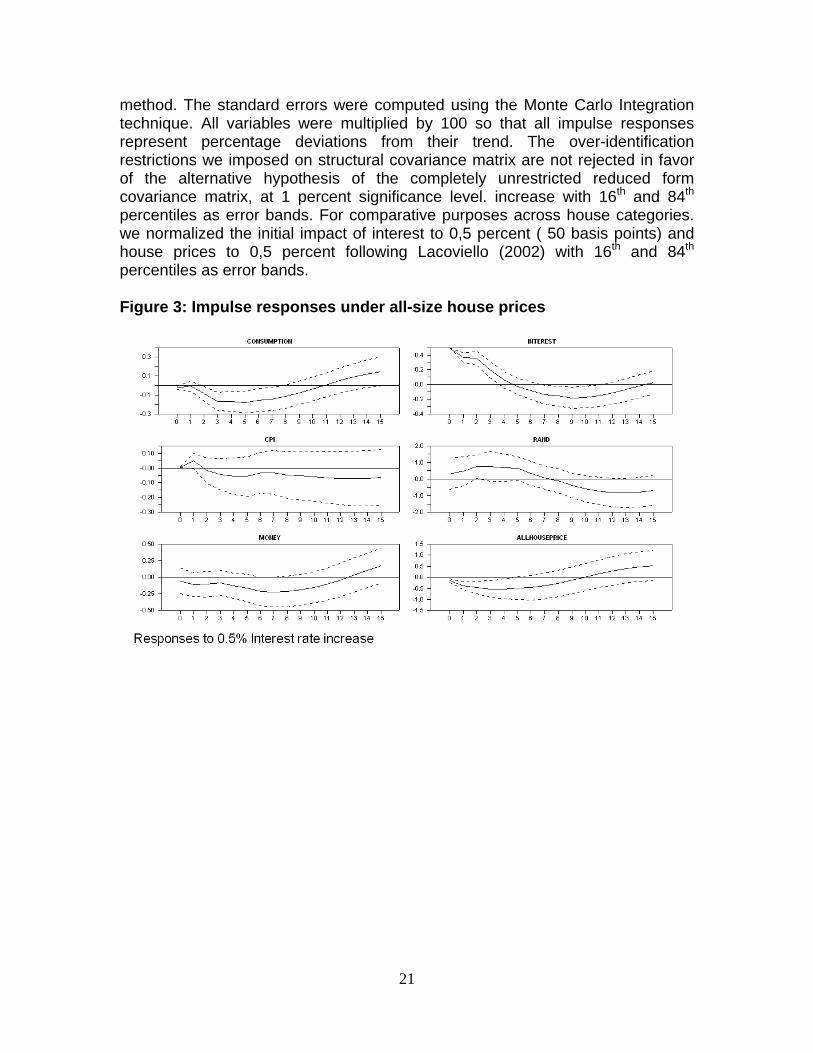
method. The standard errors were computed using the Monte Carlo Integration technique. All variables were multiplied by 100 so that all impulse responses represent percentage deviations from their trend. The over-identification restrictions we imposed on structural covariance matrix are not rejected in favor of the alternative hypothesis of the completely unrestricted reduced form covariance matrix, at 1 percent significance level. increase with 16th and 84th percentiles as error bands. For comparative purposes across house categories. we normalized the initial impact of interest to 0,5 percent ( 50 basis points) and house prices to 0,5 percent following Lacoviello (2002) with 16th and 84th percentiles as error bands. Figure 3: Impulse responses under all-size house prices

22

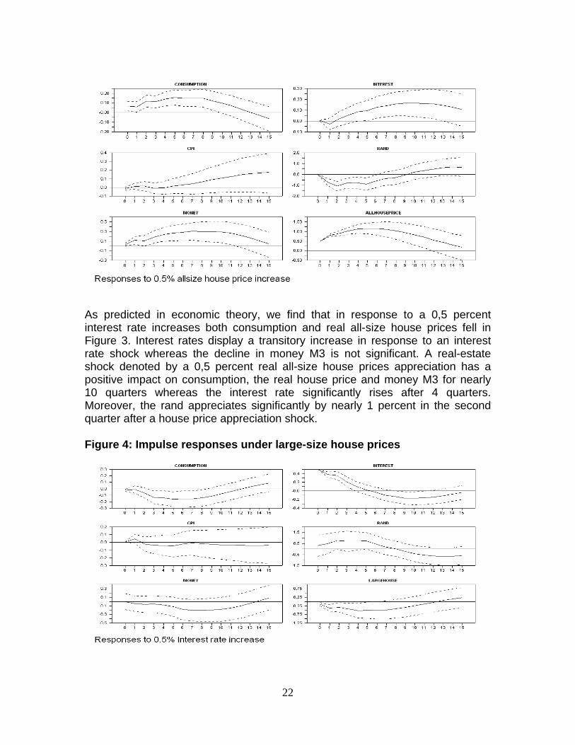
As predicted in economic theory, we find that in response to a 0,5 percent interest rate increases both consumption and real all-size house prices fell in Figure 3. Interest rates display a transitory increase in response to an interest rate shock whereas the decline in money M3 is not significant. A real-estate shock denoted by a 0,5 percent real all-size house prices appreciation has a positive impact on consumption, the real house price and money M3 for nearly 10 quarters whereas the interest rate significantly rises after 4 quarters. Moreover, the rand appreciates significantly by nearly 1 percent in the second quarter after a house price appreciation shock. Figure 4: Impulse responses under large-size house prices

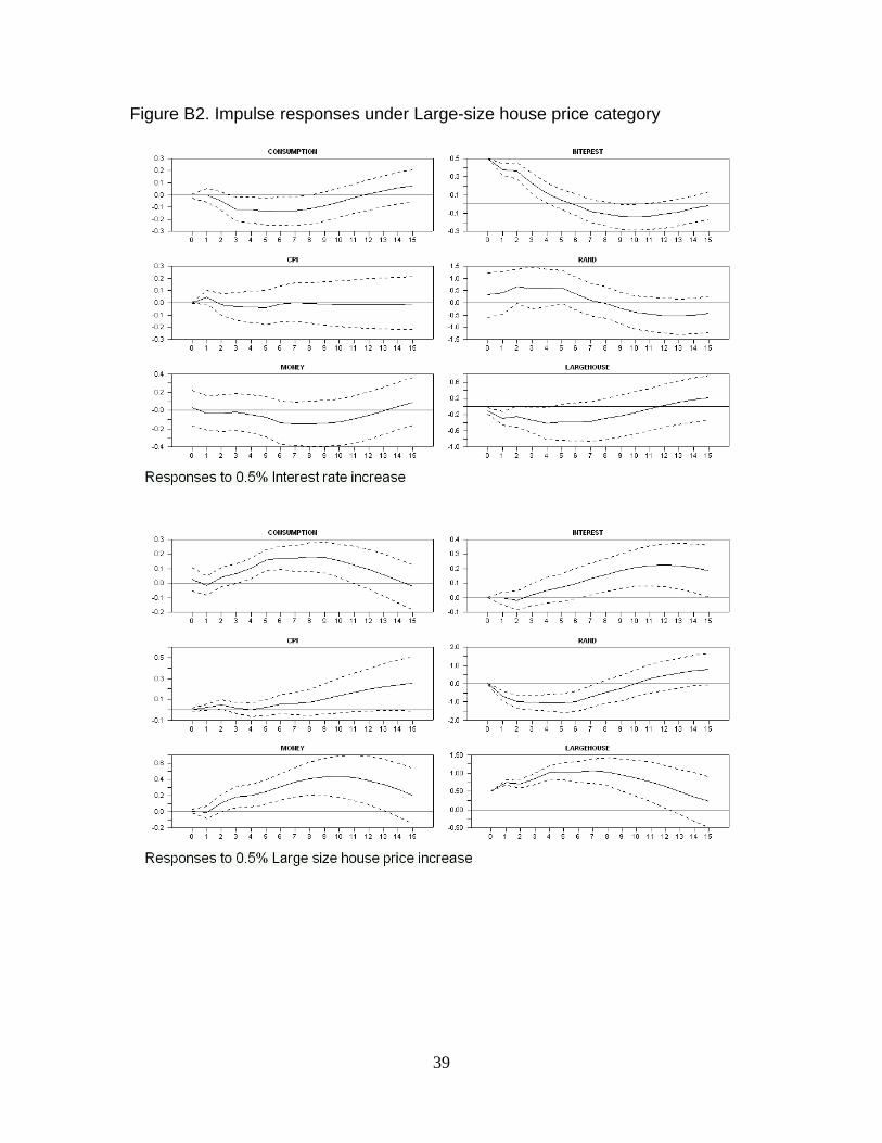
23

Figure 4 displays the impulse responses to positive interest rate and real house price shocks. Evidence shows that consumption and real house prices significantly decline and interest rates display a transitory increase after an interest rate shock. The decline in money M3 which is consistent with the liquidity effect is not significant. In addition, there is evidence that consumption, money M3, real large house prices increase following a real large-size house prices appreciation. A house appreciation also leads to a significant strengthening of the exchange rate of nearly 1 percent in the second quarter. We conclude that these responses are similar to those under the all-size house prices. Figure 5: Impulses responses under medium-size house prices

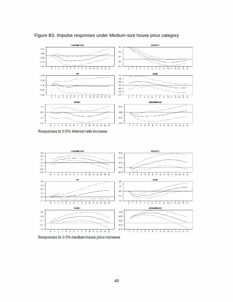
24

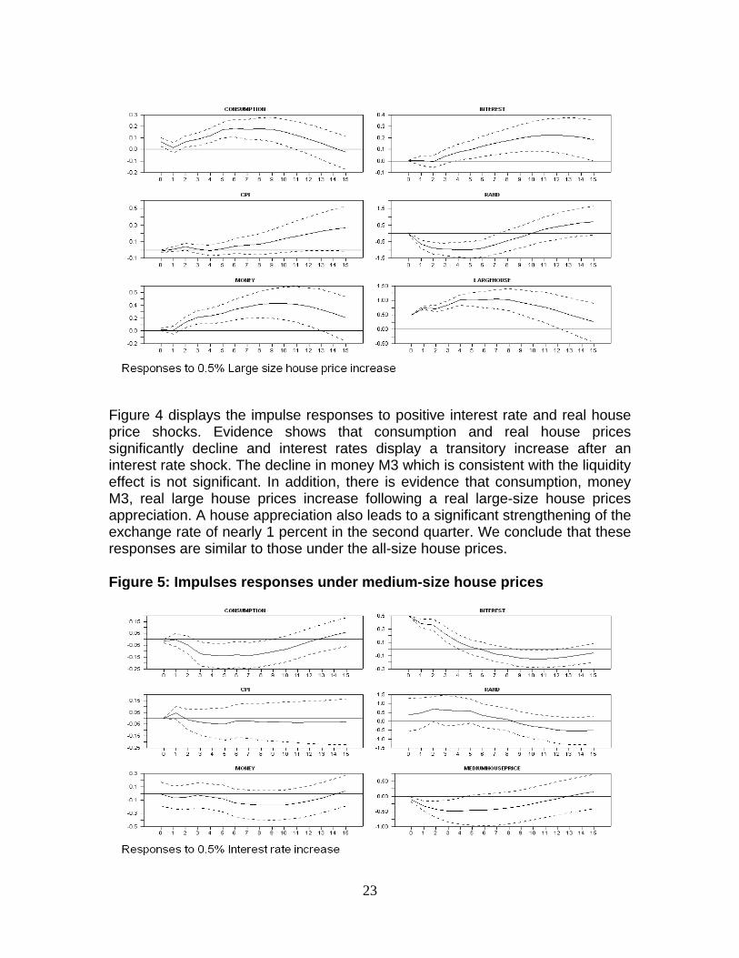
Figure 5 shows the responses of the domestic variables to a positive interest rate shock and medium sized house price shock. These responses are consistent with findings in literature indicating the U-shaped significant declines in consumption and real house price in response to interest rate shock. However, the price level declines with some delay, and money M3 remains depressed albeit insignificantly. The positive house price shock is accompanied by a rise in consumption, house price, money M3 and interest rate after some delay. Figure 6: Impulse responses under small-size house prices

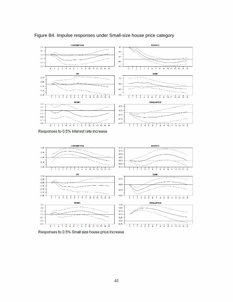
25

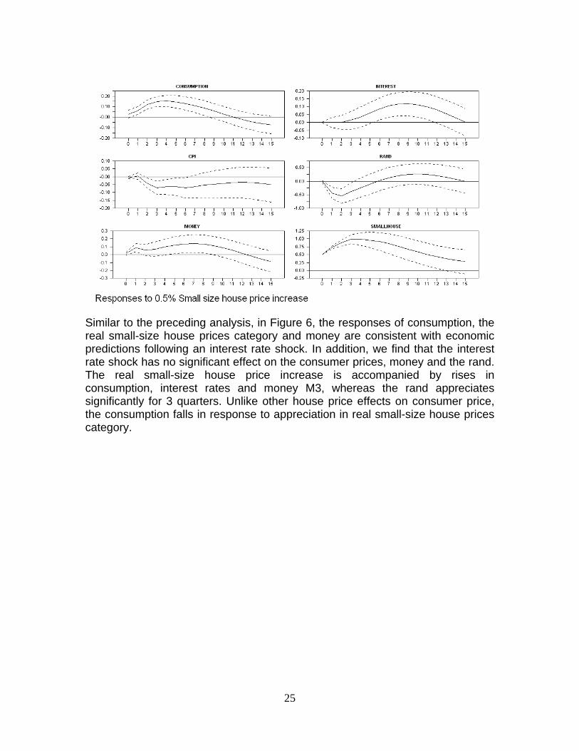
Similar to the preceding analysis, in Figure 6, the responses of consumption, the real small-size house prices category and money are consistent with economic predictions following an interest rate shock. In addition, we find that the interest rate shock has no significant effect on the consumer prices, money and the rand. The real small-size house price increase is accompanied by rises in consumption, interest rates and money M3, whereas the rand appreciates significantly for 3 quarters. Unlike other house price effects on consumer price, the consumption falls in response to appreciation in real small-size house prices category.

26

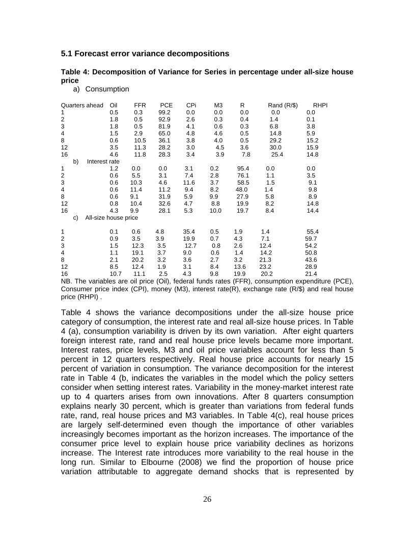
5.1 Forecast error variance decompositions Table 4: Decomposition of Variance for Series in percentage under all-size house price

a) Consumption

Quarters ahead Oil FFR PCE CPi M3 R Rand (R/$) RHPI 1 0.5 0.3 99.2 0.0 0.0 0.0 0.0 0.0 2 1.8 0.5 92.9 2.6 0.3 0.4 1.4 0.1 3 1.8 0.5 81.9 4.1 0.6 0.3 6.8 3.8 4 1.5 2.9 65.0 4.8 4.6 0.5 14.8 5.9 8 0.6 10.5 36.1 3.8 4.0 0.5 29.2 15.2 12 3.5 11.3 28.2 3.0 4.5 3.6 30.0 15.9 16 4.6 11.8 28.3 3.4 3.9 7.8 25.4 14.8

b) Interest rate 1 1.2 0.0 0.0 3.1 0.2 95.4 0.0 0.0 2 0.6 5.5 3.1 7.4 2.8 76.1 1.1 3.5 3 0.6 10.3 4.6 11.6 3.7 58.5 1.5 9.1 4 0.6 11.4 11.2 9.4 8.2 48.0 1.4 9.8 8 0.6 9.1 31.9 5.9 9.9 27.9 5.8 8.9 12 0.8 10.4 32.6 4.7 8.8 19.9 8.2 14.8 16 4.3 9.9 28.1 5.3 10.0 19.7 8.4 14.4

c) All-size house price 1 0.1 0.6 4.8 35.4 0.5 1.9 1.4 55.4 2 0.9 3.5 3.9 19.9 0.7 4.3 7.1 59.7 3 1.5 12.3 3.5 12.7 0.8 2.6 12.4 54.2 4 1.1 19.1 3.7 9.0 0.6 1.4 14.2 50.8 8 2.1 20.2 3.2 3.6 2.7 3.2 21.3 43.6 12 8.5 12.4 1.9 3.1 8.4 13.6 23.2 28.9 16 10.7 11.1 2.5 4.3 9.8 19.9 20.2 21.4 NB. The variables are oil price (Oil), federal funds rates (FFR), consumption expenditure (PCE), Consumer price index (CPI), money (M3), interest rate(R), exchange rate (R/$) and real house price (RHPI) . Table 4 shows the variance decompositions under the all-size house price category of consumption, the interest rate and real all-size house prices. In Table 4 (a), consumption variability is driven by its own variation. After eight quarters foreign interest rate, rand and real house price levels became more important. Interest rates, price levels, M3 and oil price variables account for less than 5 percent in 12 quarters respectively. Real house price accounts for nearly 15 percent of variation in consumption. The variance decomposition for the interest rate in Table 4 (b, indicates the variables in the model which the policy setters consider when setting interest rates. Variability in the money-market interest rate up to 4 quarters arises from own innovations. After 8 quarters consumption explains nearly 30 percent, which is greater than variations from federal funds rate, rand, real house prices and M3 variables. In Table 4(c), real house prices are largely self-determined even though the importance of other variables increasingly becomes important as the horizon increases. The importance of the consumer price level to explain house price variability declines as horizons increase. The Interest rate introduces more variability to the real house in the long run. Similar to Elbourne (2008) we find the proportion of house price variation attributable to aggregate demand shocks that is represented by

27

consumption is low. We do not report variance decompositions for other house categories as they show similar patterns. 5.2. Counterfactual approach We further ascertain the extent of house wealth effect on consumption using the counterfactual approach. This involves assessing the importance of the direct effect of monetary policy shock on consumption compared to the indirect effect through the endogenous effects of house wealth using the baseline and counterfactual scenarios. The baseline case allows consumption to respond to monetary policy shock and it includes the endogenous response of house wealth and its influence on consumption. We adopt the Elbourne (2008) counterfactual approach which shuts off the effects of house prices on consumption. We set the cross correlation between consumption and house prices to zero in the consumption equation of the structural model. All coefficients of 38a in each ( )LA matrix in equation [1] are set to zero and other parameters remain as originally estimated. The impulse responses are then recalculated to construct an alternative impulse response for consumption. The difference between the two consumption responses under two scenarios is a measure of the contribution of the consumption wealth channel in the transmission channel of monetary policy (Lettau and Ludvigson 2001b). However, Elbourne (2008) argues that this counterfactual approach is subject to the Lucas critique when consumption does not depend on house price, suggesting that the central bank would have reacted differently and the monetary policy shocks would be different. However, we are not looking at what would happen if consumption did not depend on house prices but we focus on the proportion of the response estimated to come through house prices. Thus the Lucas critique would not be so strong and these results should be taken as a form of circumstantial evidence (Elbourne 2008, Giuliodori 2005). 5.3 Robustness analysis As robustness analysis, we add the restrictions that house prices respond to both aggregate demand and aggregate supply in the baseline model to check the robustness of the role house wealth on consumption, denoted by the equation [10].

28

Alternative Model

[10]

⎥⎥⎥⎥⎥⎥⎥⎥⎥⎥⎥

⎦

⎤

⎢⎢⎢⎢⎢⎢⎢⎢⎢⎢⎢

⎣

⎡

HPI

R

MS

MD

P

PCE

FFR

OIL

εεεεεεεε

$/

=

⎥⎥⎥⎥⎥⎥⎥⎥⎥⎥⎥

⎦

⎤

⎢⎢⎢⎢⎢⎢⎢⎢⎢⎢⎢

⎣

⎡

100001010000100000010

000010000000100000001

86858483

677574737271

67656261

565453

4341

3831

21

aaaaaaaaaa

aaaaaaa

aaaa

a

⎥⎥⎥⎥⎥⎥⎥⎥⎥⎥⎥

⎦

⎤

⎢⎢⎢⎢⎢⎢⎢⎢⎢⎢⎢

⎣

⎡

HPI

R

R

M

P

PCE

FFR

OIL

uuuuu

uuu

$/

5.4 Discussion of results We report the results in Table 5 from the Elbourne approach and its modified version for the four house categories separated into baseline models, alternative models and their counterfactual models. The impulse responses from the alternative models in Appendix B are similar to their counterparts in the baseline models. Similarly, the counterfactual responses do not show significant differences compared to both the baseline and alternative model. Table 5: Percentages declines in consumption by house categories in the sixth quarter

a) Baseline model Main results Counterfactual Results House size Elbourne Modified Elbourne Elbourne Modified Elbourne All-size 9.8% 6.3% 8.55% 5.3% Large-size 5.3% 5.2% 4.4% 4.3% Medium-size 4.7% 4.2% 3.8% 3.3% Small-size 3.7% 4.0% 3.2% 3.4%

b) Alternative model All-size 11.5% 7.2% 10.5% 6.5% Large-size 5.6% 5.4% 5.0% 4.9% Medium-size 5.1% 4.4% 4.6% 4.0% Small-size 3.5% 3.7% 3.6% 3.8% NB. These percentages refer to effects in the sixth quarter from corresponding house categories. More detailed information on these calculations is attached in the table C1-C4 in Appendix C under four house categories The results reported in Table 5 show the percentage of consumption decline attributed to the combined effect of house wealth and credits associated with an interest increase at the peak of interest rate effect on consumption in the sixth quarter. These percentages were calculated using the Elbourne approach defined in equation [7] and the modified version in equation [9]. As such we report the results for both the baseline model and the counterfactual model in table 5. We illustrate how we calculate the consumption decline using both

29

Elbourne and its modified version. The detailed information on impulse response and the quantified magnitudes over time periods are found in Appendix C. For example in tables C1–C4 in Appendix C,18 following a monetary policy shock, consumption declines by 0,18 percent and real house prices decline by 0,49 percent. In addition, all-size house price increase by 1,54 percent and consumption increases by 0,27 percent following a 0,5 percent real all-size house prices shock. We deduce nearly 9,8 percent and 6,3 percent of the consumption declines are due to the combined role of housing wealth and a housing credit channel using the Elbourne approach and its modified version respectively. 19 The declines from the counterfactual model with respect to all-size house are 8,55 percent and 5,32 percent respectively.20 Moreover, the percentage of consumption declines under the all-size house category in table 5(a) is greater than the 5,3 percent for large size, 4,7 percent in the medium size and 3,7 percent in the small-size house using the Elbourne approach. A similar trend is visible using the modified version.21 We validate the findings above by reporting consumption declines in the sixth quarter from the alternative model in Table 5(b) as calculated in the tables C1–C4 in Appendix C. Like before, we reach a similar conclusion as in the baseline model that consumption declined by 11,5 percent in the all-size house price, which is larger than 5,6 percent in large-size, 5,1 percent in medium-size and 3,5 percent in the small-size house price using the Elbourne approach. The percentage declines do not deviate significantly from the counterfactual results. The findings suggest that house wealth and credits explain a small percentage of consumption declines in response to interest rate increase. Perhaps this outcome could be attributed to the response of house wealth to its own innovation which does not appear highly transitory. We also used the counterfactual approach to validate the importance of the house wealth channel on consumption. That is, we assessed whether there was any significant evidence on the role of house wealth in propagating consumption declines in all four house categories. Figure 7 shows the comparison of impulse

18 These are selected impulses responses from figures 3–6 and figures B1–B4 in Appendix B. 19 The aim is show how the values are calculated using formulas defined in equation [7] and equation [9]. For example the calculation for the all-size house price category using the Elbourne approach is 9,8% = ((-0.18/-0,49) x0.27)x100. The modified Elbourne approach values of 6,3% =((-0,18/-0,49)x(0,27/1.54))x100. These values have been rounded to the two decimal points. 20 The detailed calculations of these values are available in tables attached in the Appendix. The tables in the appendix give only information of selected impulse responses used specifically in the calculations using both Elbourne and Modified Elbourne versions. The impulse responses under the baseline line models and the alternative are exactly, from figures 3–6 and figures B1-B4 in the appendix for alternative model. The full impulse responses of counterfactual are not attached as they are similar to those in baseline and alternative model. 21 Results not reported here show that proportion of consumption decline attributed to the combined house wealth and credits are larger using recursive VAR approach. Elbourne (2008) identified similar discrepancy when comparing his SVAR results to those from VAR using Choleski decomposition in Giuliodori (2005).

30

response functions of consumption under the baseline and the counterfactual models according to four house-size categories in response to 0,5 percent (50 basis points) interest rate increase. The Baseline model shows the total effect of interest rate shocks on consumption, including those simulated by the endogenous responses of house wealth. In contrast, the counterfactual models simulate effects of interest rate shock on consumption by shutting off the wealth effect to consumption as described in the preceding section. All the impulse responses of consumptions of the four house categories under the baseline models are close to those under the counterfactual model, and the impulses from the latter are within the same 16th and 84th percentile error bands of the baseline models. Hence, given the margin of error these counterfactual consumption and interest rate impulse responses are not different from the baseline responses. This finding suggests that a substantial portion of the real effects of interest rate shocks on consumption are relatively attributable to effects operating through other channels other than the house wealth channel. However, this finding does not imply that house wealth has no effect on consumption. It means that the endogenous changes in house wealth driven by innovation in interest rates have little marginal effects on consumption. This could be due to the interest rate shock which is highly transitory and significant for only five quarters in both the counterfactual and the baseline models. The similarities and the insignificant gap between the impulse responses of consumption in response to interest rate shocks under the baseline and counterfactual models provide little support for the view that the wealth channel is the dominant source of monetary transmission to consumption. Perhaps this is linked to the transitory effect of interest rate shock on real house which significantly dies out in 5 quarters or 15 months and interest rate shocks on its movements are highly transitory. It is argued in Ludvigson et al. (2002) that such transitory changes in wealth have little, if any, impact on consumer spending. Furthermore, as indicated by Ludvigson et al’s (2001b) results, when movements in consumption occur only in response to permanent changes in asset values, the wealth channel of monetary policy transmission to consumption would probably be quite small, which is consistent with our findings. We also found that the response of wealth in relation to its innovation looks not entirely transitory (in figure 3–6 and figures B1–B4). This could mean that it is a mixture of permanent shocks to which consumption may be responding to, whereas the transitory shock has little influence on consumption spending. The impulse responses from the alternative model in the Figure D1 in Appendix D leads to a similar conclusion strengthening credibility that these conclusions are robust to restrictions imposed.

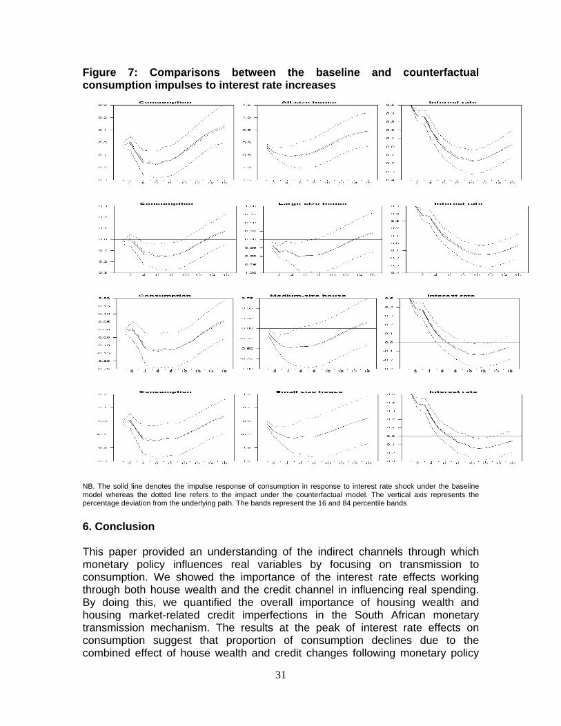
31

Figure 7: Comparisons between the baseline and counterfactual consumption impulses to interest rate increases

NB. The solid line denotes the impulse response of consumption in response to interest rate shock under the baseline model whereas the dotted line refers to the impact under the counterfactual model. The vertical axis represents the percentage deviation from the underlying path. The bands represent the 16 and 84 percentile bands 6. Conclusion This paper provided an understanding of the indirect channels through which monetary policy influences real variables by focusing on transmission to consumption. We showed the importance of the interest rate effects working through both house wealth and the credit channel in influencing real spending. By doing this, we quantified the overall importance of housing wealth and housing market-related credit imperfections in the South African monetary transmission mechanism. The results at the peak of interest rate effects on consumption suggest that proportion of consumption declines due to the combined effect of house wealth and credit changes following monetary policy

32

tightening is 9,8 percent in all-size, 3,7 percent in small-size, 4,7 percent in medium-size and 5,3 percent in large-size houses. Thus, interest rate effects operating through house wealth and the credit channel are felt differently by the four house categories. Consumption declines by a large proportion under the large-size compared to the small-size category. Moreover, the differences between the consumption impulse responses from the counterfactual and baseline scenarios provide little support that combined house wealth and credit effect channels are the dominant sources of monetary policy transmission to consumption. These findings suggest that the direct effects of high interest rates on consumption appear to be more important in transmitting monetary policy to the economy than through the indirect effects. Hence, monetary policy tightening can marginally weaken inflationary pressures arising from excessive consumption operating through house wealth and the credit channel. References Aoki,k., Proudman, J., Vlieghe G., (2002). “House as collateral: Has the link between house prices and consumption in the U.K. changed?” Fed reserve Bank New York economic policy review 8 (1), 163-177 Aoki,k., Proudman, J., Vlieghe G., (2004). “House prices, consumption and monetary policy: a financial accelator approach”, Journal of Financial Intermediation 13, 144-435 Bernanke, B., Blinder, A., (1998),“Credit, money, and aggregate demand”, American Economic Review 78(2), 435-339. Bernanke , B., Gertler, M., (1995), “Inside the black box: The credit channel of monetary transmission”, Journal of Economic Perspectives. 9 (4), 27-48. Blanchard, O., Perotti, R., (2002), “An empirical characterization of the dynamic effects of changes in government spending and taxes on output”, Quarterly Journal of Economics, 117, 1329–1368. Brischetto, A., Voss, G., (1999), “A Structural Vector Autoregression Model of Monetary Policy in Australia”, RBA Research Discussion Paper No 1999-11. Calza, A., Monacelli, T., Straca, L.,(2007), “Mortgage Markets, collateral Constraints, and monetary policy: Do Institutional Factors Matter?”, Center for financial studies. Working paper 2007/10 Case, K. E., Quigley, J. M., Shiller, R. J., (2005), “Comparing wealth effects: The stock Market versus the housing market”, B.E. Journals of Macroeconomics: Advances in Macroeconomics, 2005, Vol. 5 Issue 1, preceding p1-32, 33p Chirinko, R. S., De Hann, L., Sterken, E., (2004), “Asset Price shocks, Real expenditure and financial structure: A multi country Analysis”, De Netherlands working Paper 14

33

Elbourne , A., (2008), “The UK housing market and the monetary policy transmission mechanism: An SVAR approach”, Journal of Housing Economics, Volume 17, Issue 1, March 2008, Pages 65-87 Enders, W. (2004), Applied econometric time series, Second edition, John Wiley & Sons, Inc Faust, J., Leeper, E., (1997), “When do long run identifying restrictions give reliable results?”, Journal of Business Economic Statistics.15, 345 -353 Fuller, W. A. (1976). Introduction to Statistical Time Series. New York:Wiley Gottschalk, J., (2001), “An Introduction into the SVAR Methodology: Identification, Interpretation and Limitations of SVAR models ”, Kiel Working Paper No. 1072 Giuliodori, M., (2005), “Monetary policy shocks and the role of house prices across European Countries”, Scottish Journal of Political Economy 52 (4), 519-543 Gupta, R., Kabundi, K., (2010), “The effect of monetary policy on real house price growth in South Africa: A factor Augmented Vector Auto regression (FAVAR) Approach”, Economic modelling, HM Treasury, (2003), “Housing, Consumption and EMU. EMU study”, HM Treasury, London Kasai, N., Gupta, R., (2010). "Financial Liberalization and the Effectiveness of Monetary Policy on House Prices in South Africa," The IUP Journal of Monetary Economics, vol. 8, Issue 4, pages 59-74 Kimi, S., Roubini, N., (2000), “Exchange rate anomalies in the industrial countries: A solution with the structural VAR approach”, Journal of Monetary Economics 45 (3), 561-586. Lacoviello, M., (2002), “House Prices and Business Cycle in Europe”, Aver Analysis. Boston College Working Paper 540. Lacoviello, M., (2004), “Consumption, house prices, and collateral constraints: A structural econometric analysis”, Journal of Housing Economics 13, 304-320 Lacoviello, M., Minnetti, R., (2007), “The credit Channel of monetary policy: Evidence from the housing Market”, Journal of Macroeconomics., in press Ludvigson,S., Stendel, C., Lettau, M., (2002), “Understanding trend and cycle in Asset values : Bulls, Bears, and the Wealth effect on consumption. ”, Unpublished paper, New York University Ludvigson,S., Stendel, C., Lettau, M., (2002), “Monetary policy transmission through consumption wealth channel”, Federal Reserve Bank New York Economic Policy Review 8 (1), 117-133.

34

Maclennan, D., Muellbauer,J., Stephens, M., (2000), “Asymmetries in housing and financial market institutions and EMU”. McCarthy, J., Peach, R.W., (2002), “Monetary policy transmission to residential investment”, Federal Reserve Bank New York Economic Policy Review 8 (1), 139-158. Phillips, P.C.B., (1998), “Impulse response and forecast error variance decompositions in non-stationary VARs”, Journal of Econometrics 83, 21-56 Ramirez, J. F. R., Waggoner D. F., Zha T (2009), “Structural Vector Autoregressions: Theory of identification and Algorithms for inference”, Review of Economic Studies, Vol. 77, No. 2. (2010), pp. 665-696. Sims, C., Zha, T., (2006), “Does Monetary policy generate recessions?”, Macroeconomics Dynamics 10 (2), 231-272.

35

Appendix A 3.2. Deriving formulas This section mainly highlights how we derived the Elbourne and its modified formulas and relies on the Vector moving averages (VMA) representation. We specifically focus on the consumption and house price equations. Firstly we denote the vector ⎥

⎦

⎤⎢⎣

⎡=

t

tt h

cM where tc is the consumption

and th is the real house price variables. The structural form equation can be written as [A1] ttt MBM εψψ ++= −110

were ⎥⎦

⎤⎢⎣

⎡=

11

21

12

bb

B ⎥⎦

⎤⎢⎣

⎡=

20

100 b

bψ

⎥⎦

⎤⎢⎣

⎡=

2221

12111 bb

bbψ ⎥

⎦

⎤⎢⎣

⎡=

ht

ctt ε

εε

Then normalizing [A1] by B to get the reduced form equation [A2] [A2] ttt eMAAM ++= −110

were ⎥⎦

⎤⎢⎣

⎡== −

20

100

10 a

aBA ψ , ⎥

⎦

⎤⎢⎣

⎡== −

2221

12111

11 aa

aaBA ψ and ⎥

⎦

⎤⎢⎣

⎡== −

ht

cttt e

eBe ε1

After some mathematical manipulation following the derivations in Enders (2004) which used a bivariate equation expressed in VMA with reduced form error

[A3] ⎥⎦

⎤⎢⎣

⎡+⎥

⎦

⎤⎢⎣

⎡=⎥

⎦

⎤⎢⎣

⎡

−

−∞

=∑ ⎥

⎦

⎤⎢⎣

⎡ith

itc

i

i

t

t

ee

hc

hc

aaaa

02221

1211v

Replacing reduced from error in [A3] by structural innovations leads to [A4]

[A4] ⎥⎦

⎤⎢⎣

⎡⎥⎦

⎤⎢⎣

⎡+⎥

⎦

⎤⎢⎣

⎡=⎥

⎦

⎤⎢⎣

⎡

−

−∞

=∑

ith

itc

it

t

iiii

hc

hc

εε

φφφφ

0 2221

1211

)()()()(

v

The above form allows derivations of the impact multipliers in tracing the impact of a one unit change in structural innovation. For example the impact effect of

iht −ε on itc − and ith −

[A5] )(12 iddc

iht

it φε

=−

− )(22 iddh

iht

it φε

=−

−

Using the above the impact multipliers we can trace the wealth effects of house price increases on consumption, and combined wealth effects and credits effects

36

of interest on reducing consumption expenditure. We use a simplified consumption equation below. In equation [A6] consumption tc depends upon real house prices th [A6] ttt uwhc += were w is house wealth coefficient and tu is the error term. The wealth effect or effect of house price on consumption is given by equation [A7]

[A7] wdhdc

t

t =

Mathematically, we can express equation [A7] in a form which introduces the impact multiplier effects after adjusting for specific shocks effects which leaves equation [A7] mathematical unchanged. This mathematically correct transformation gives the numerator and denominator an economic meaning. Hence, we express the effects of house price increases on consumption in equation [A7] with the numerator representing the impact of house price shock on consumption and the denominator denoting the impact of house shock on house prices as in equation [A8]

[A8] w

ddh

ddc

ht

t

ht

t

=

ε

ε

The

ht

t

ddcε

and ht

t

ddhε

denotes the impact of house price shocks on consumption

and house price respectively. Similarly, we can introduce the effects of interest rates, with the

rt

t

ddcε

and rt

t

ddhε

representing the interest rate effects on

consumption and house price respectively. We divide equation [A6] by consumption to quantify the separate contributions from the combined wealth coefficient and house price terms )( tt cwh from those associated with the residual term )( tt cu . Subsequently using )( tt cwh , we can express the proportion of declines in consumption, linked to combined house wealth and credits effects associated with interest rates increases using equation [A9] to get the modified Elbourne approach denoted by mQ . We use this to trace the wealth and credits effects arising from an interest rate increase.

37

[A9]

rt

t

rt

t

t

tm

ddc

ddh

WdcdhWQ

ε

ε*==

The preceding approach differs from Elbourne (2008) approach denoted by Q in equation [A10] which ignores the denominator in equation [A8].

[A9]

rt

t

rt

t

ht

t

ddc

ddh

ddcQ

ε

εε

*=

38

Appendix B. Impulse response under the Alternative model Figure B1. Impulse responses under All-size house price category

39

Figure B2. Impulse responses under Large-size house price category

40

Figure B3. Impulse responses under Medium-size house price category

41

Figure B4. Impulse responses under Small-size house price category

42

Appendix C. Consumption declines in percentage for all house price categories Table C1. Percentage consumption declines under All-size house price category

a) Baseline model Main model Counterfactual Model

ci→ hi→ ch→ hh→ Elbourne Mod. Elbourne ci→ hi→ ch→ hh→ Elbourne Mod. Elbourne 1 -0.02 -0.14 0.08 0.50 1.1% 2.2% 0 -0.14 0.00 0.50 0.0% 0.0% 2 0.00 -0.38 0.04 0.91 0.0% 0.0% 0.01 -0.38 -0.01 0.93 0.0% 0.0% 3 -0.09 -0.47 0.17 1.12 3.1% 2.7% -0.07 -0.47 0.12 1.14 1.8% 1.6% 4 -0.17 -0.53 0.19 1.33 5.9% 4.4% -0.15 -0.54 0.15 1.37 4.0% 3.0% 5 -0.16 -0.53 0.22 1.49 6.8% 4.6% -0.15 -0.55 0.19 1.54 5.3% 3.4% 6 -0.18 -0.49 0.27 1.54 9.8% 6.3% -0.17 -0.51 0.26 1.61 8.6% 5.3% 7 -0.15 -0.46 0.26 1.51 8.7% 5.8% -0.15 -0.49 0.25 1.59 7.7% 4.8% 8 -0.14 -0.37 0.24 1.42 9.1% 6.4% -0.14 -0.41 0.24 1.51 8.2% 5.5% 9 -0.11 -0.25 0.22 1.28 9.8% 7.7% -0.11 -0.29 0.23 1.38 9.0% 6.6% 10 -0.07 -0.12 0.19 1.08 10.8% 10.0% -0.08 -0.16 0.20 1.17 9.6% 8.2% 11 -0.03 0.03 0.14 0.85 -13.4% -15.7% -0.04 -0.02 0.16 0.94 33.1% 35.4% 12 0.01 0.16 0.09 0.61 0.8% 1.3% 0.00 0.11 0.10 0.69 0.0% 0.0%

b) Alternative model

1 0.00 -0.09 0.02 0.50 0.1% 0.1% 0.00 -0.09 0.00 0.50 0.0% 0.0% 2 0.01 -0.29 0.00 0.93 0.0% 0.0% 0.01 -0.30 -0.01 0.93 0.0% 0.0% 3 -0.06 -0.36 0.14 1.15 2.4% 2.1% -0.06 -0.37 0.12 1.14 2.0% 1.7% 4 -0.14 -0.41 0.16 1.38 5.6% 4.1% -0.14 -0.42 0.15 1.36 4.9% 3.6% 5 -0.14 -0.39 0.20 1.55 7.2% 4.6% -0.14 -0.40 0.19 1.54 6.5% 4.2% 6 -0.15 -0.35 0.27 1.61 11.6% 7.2% -0.15 -0.36 0.26 1.61 10.5% 6.5% 7 -0.12 -0.32 0.26 1.58 10.2% 6.5% -0.12 -0.33 0.25 1.59 9.3% 5.9% 8 -0.12 -0.25 0.25 1.50 11.7% 7.8% -0.12 -0.27 0.24 1.51 10.6% 7.0% 9 -0.09 -0.14 0.24 1.36 15.3% 11.2% -0.09 -0.17 0.23 1.38 13.3% 9.7% 10 -0.05 -0.03 0.20 1.15 40.9% 35.6% -0.06 -0.06 0.20 1.17 20.8% 17.7% 11 -0.02 0.09 0.15 0.90 -3.7% -4.1% -0.03 0.06 0.16 0.94 -6.6% -7.0% 12 0.02 0.20 0.10 0.64 0.8% 1.2% 0.01 0.17 0.10 0.69 0.7% 1.1% NB. ci→ , hi→ refers to impact of a 0.5% (50 basis points) interest rate i increase on consumption c and house price h . ch→ , hh→ refers to impact of 0.5% house price h increase on consumption c and house price h . Mod. Elbourne refers to the modified Elbourne approach from equation [9] in the main text. The shaded parts represent the maximum impact of interest rate increase on consumption. For example the percentage of consumption decline due to combined role of house-wealth and credit effects at this point baseline model using Elbourne formula is 9.8% i.e ((-0.18/-0.49)x0.27)x100; Using the modified Elbourne approach gives 6.3% i.e ((-0.18/-0.49)x(0.27/1.54))x100. Similarly all calculations are done the same way.

43

Table C2. Percentage consumption declines under large-size house price category a) Baseline model

Main model Counterfactual Model ci→ hi→ ch→ hh→ Elbourne Mod. Elbourne ci→ hi→ ch→ hh→ Elbourne Mod. Elbourne 1 -0.02 -0.16 0.07 0.50 0.8% 1.5% 0.00 -0.16 0.00 0.50 0.0% 0.0% 2 -0.01 -0.38 0.01 0.75 0.0% 0.0% 0.01 -0.36 -0.03 0.74 0.1% 0.1% 3 -0.06 -0.33 0.07 0.71 1.3% 1.8% -0.04 -0.31 0.03 0.70 0.4% 0.5% 4 -0.13 -0.43 0.09 0.84 2.7% 3.3% -0.11 -0.41 0.05 0.83 1.3% 1.6% 5 -0.14 -0.52 0.12 1.00 3.1% 3.1% -0.12 -0.51 0.09 1.00 2.1% 2.1% 6 -0.16 -0.49 0.16 1.01 5.3% 5.2% -0.15 -0.48 0.15 1.02 4.4% 4.3% 7 -0.15 -0.47 0.18 0.99 5.6% 5.6% -0.14 -0.48 0.16 1.02 4.7% 4.7% 8 -0.15 -0.46 0.17 1.00 5.3% 5.3% -0.14 -0.46 0.16 1.04 4.9% 4.7% 9 -0.13 -0.39 0.17 0.96 5.7% 5.9% -0.13 -0.39 0.17 1.02 5.6% 5.5% 10 -0.10 -0.30 0.16 0.86 5.5% 6.4% -0.11 -0.31 0.17 0.93 5.7% 6.2% 11 -0.07 -0.22 0.13 0.76 4.2% 5.5% -0.07 -0.22 0.14 0.84 4.8% 5.7% 12 -0.03 -0.11 0.10 0.66 3.0% 4.6% -0.04 -0.12 0.12 0.75 3.6% 4.9%

b) Alternative model 1 0.00 -0.12 0.03 0.50 0.1% 0.2% 0.00 -0.12 0.00 0.50 0.0% 0.0% 2 0.00 -0.30 -0.01 0.75 0.0% 0.0% 0.00 -0.29 -0.03 0.74 0.0% 0.1% 3 -0.05 -0.25 0.04 0.71 0.9% 1.2% -0.04 -0.24 0.03 0.70 0.5% 0.7% 4 -0.12 -0.33 0.07 0.84 2.3% 2.8% -0.11 -0.34 0.05 0.83 1.6% 1.9% 5 -0.12 -0.42 0.10 1.00 2.9% 2.9% -0.11 -0.42 0.09 1.00 2.4% 2.4% 6 -0.14 -0.38 0.15 1.02 5.6% 5.4% -0.13 -0.38 0.15 1.02 5.0% 4.9% 7 -0.13 -0.38 0.17 1.01 5.8% 5.7% -0.12 -0.37 0.16 1.02 5.4% 5.3% 8 -0.13 -0.36 0.16 1.03 5.9% 5.7% -0.13 -0.37 0.16 1.04 5.5% 5.3% 9 -0.12 -0.29 0.17 1.00 6.8% 6.8% -0.12 -0.31 0.17 1.02 6.5% 6.3% 10 -0.09 -0.22 0.16 0.90 6.8% 7.6% -0.09 -0.24 0.17 0.93 6.5% 6.9% 11 -0.06 -0.14 0.14 0.80 5.6% 7.1% -0.06 -0.16 0.15 0.84 5.2% 6.2% 12 -0.02 -0.05 0.11 0.69 5.0% 7.3% -0.03 -0.08 0.12 0.75 4.1% 5.5% NB. ci→ , hi→ refers to impact of a 0.5% (50 basis points) interest rate i increase on consumption c and house price h . ch→ , hh→ refers to impact of 0.5% house price h increase on consumption c and house price h .Mod. Elbourne refers to the modified Elbourne approach from equation [9] in the main text. The shaded parts represent the maximum impact of interest rate increase on consumption. For example the percentage of consumption decline due to combined role of house-wealth and credit effects at this point baseline model using Elbourne formula is 5.3% i.e ((-0.16/-0.49)x0.16)x100; Using the modified Elbourne approach gives 5.2% i.e ((-0.16/-0.49)x(0.16/1.01))x100. Similarly all calculations are done the same way.

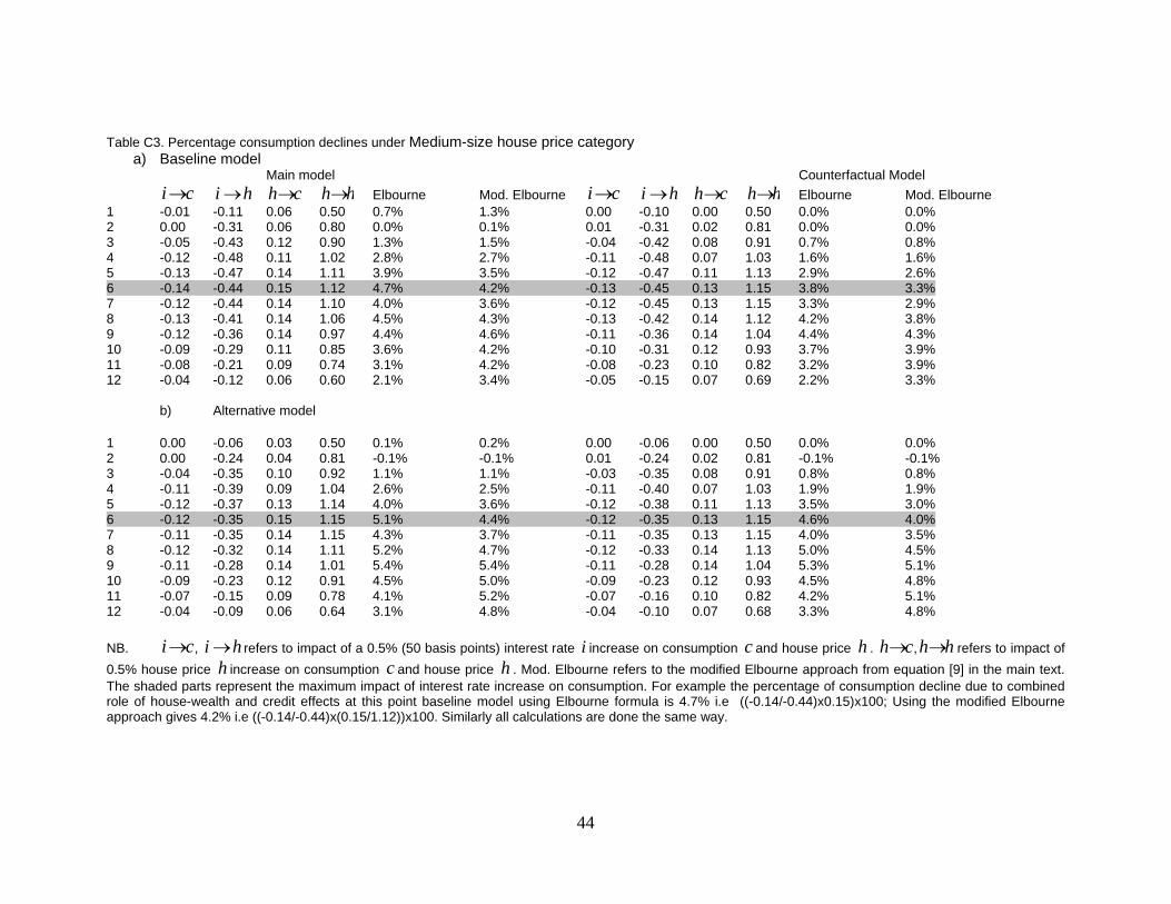
44

Table C3. Percentage consumption declines under Medium-size house price category a) Baseline model

Main model Counterfactual Model ci→ hi→ ch→ hh→ Elbourne Mod. Elbourne ci→ hi→ ch→ hh→ Elbourne Mod. Elbourne 1 -0.01 -0.11 0.06 0.50 0.7% 1.3% 0.00 -0.10 0.00 0.50 0.0% 0.0% 2 0.00 -0.31 0.06 0.80 0.0% 0.1% 0.01 -0.31 0.02 0.81 0.0% 0.0% 3 -0.05 -0.43 0.12 0.90 1.3% 1.5% -0.04 -0.42 0.08 0.91 0.7% 0.8% 4 -0.12 -0.48 0.11 1.02 2.8% 2.7% -0.11 -0.48 0.07 1.03 1.6% 1.6% 5 -0.13 -0.47 0.14 1.11 3.9% 3.5% -0.12 -0.47 0.11 1.13 2.9% 2.6% 6 -0.14 -0.44 0.15 1.12 4.7% 4.2% -0.13 -0.45 0.13 1.15 3.8% 3.3% 7 -0.12 -0.44 0.14 1.10 4.0% 3.6% -0.12 -0.45 0.13 1.15 3.3% 2.9% 8 -0.13 -0.41 0.14 1.06 4.5% 4.3% -0.13 -0.42 0.14 1.12 4.2% 3.8% 9 -0.12 -0.36 0.14 0.97 4.4% 4.6% -0.11 -0.36 0.14 1.04 4.4% 4.3% 10 -0.09 -0.29 0.11 0.85 3.6% 4.2% -0.10 -0.31 0.12 0.93 3.7% 3.9% 11 -0.08 -0.21 0.09 0.74 3.1% 4.2% -0.08 -0.23 0.10 0.82 3.2% 3.9% 12 -0.04 -0.12 0.06 0.60 2.1% 3.4% -0.05 -0.15 0.07 0.69 2.2% 3.3%

b) Alternative model 1 0.00 -0.06 0.03 0.50 0.1% 0.2% 0.00 -0.06 0.00 0.50 0.0% 0.0% 2 0.00 -0.24 0.04 0.81 -0.1% -0.1% 0.01 -0.24 0.02 0.81 -0.1% -0.1% 3 -0.04 -0.35 0.10 0.92 1.1% 1.1% -0.03 -0.35 0.08 0.91 0.8% 0.8% 4 -0.11 -0.39 0.09 1.04 2.6% 2.5% -0.11 -0.40 0.07 1.03 1.9% 1.9% 5 -0.12 -0.37 0.13 1.14 4.0% 3.6% -0.12 -0.38 0.11 1.13 3.5% 3.0% 6 -0.12 -0.35 0.15 1.15 5.1% 4.4% -0.12 -0.35 0.13 1.15 4.6% 4.0% 7 -0.11 -0.35 0.14 1.15 4.3% 3.7% -0.11 -0.35 0.13 1.15 4.0% 3.5% 8 -0.12 -0.32 0.14 1.11 5.2% 4.7% -0.12 -0.33 0.14 1.13 5.0% 4.5% 9 -0.11 -0.28 0.14 1.01 5.4% 5.4% -0.11 -0.28 0.14 1.04 5.3% 5.1% 10 -0.09 -0.23 0.12 0.91 4.5% 5.0% -0.09 -0.23 0.12 0.93 4.5% 4.8% 11 -0.07 -0.15 0.09 0.78 4.1% 5.2% -0.07 -0.16 0.10 0.82 4.2% 5.1% 12 -0.04 -0.09 0.06 0.64 3.1% 4.8% -0.04 -0.10 0.07 0.68 3.3% 4.8% NB. ci→ , hi→ refers to impact of a 0.5% (50 basis points) interest rate i increase on consumption c and house price h . ch→ , hh→ refers to impact of 0.5% house price h increase on consumption c and house price h . Mod. Elbourne refers to the modified Elbourne approach from equation [9] in the main text. The shaded parts represent the maximum impact of interest rate increase on consumption. For example the percentage of consumption decline due to combined role of house-wealth and credit effects at this point baseline model using Elbourne formula is 4.7% i.e ((-0.14/-0.44)x0.15)x100; Using the modified Elbourne approach gives 4.2% i.e ((-0.14/-0.44)x(0.15/1.12))x100. Similarly all calculations are done the same way.

45

Table C4. Percentage consumption declines under Small-size house price category a) Baseline model

Main model Counterfactual Model ci→ hi→ ch→ hh→ Elbourne Mod. Elbourne ci→ hi→ ch→ hh→ Elbourne Mod. Elbourne 1 -0.01 -0.11 0.03 0.50 0.2% 0.5% 0.00 -0.11 0.00 0.50 0.0% 0.0% 2 0.00 -0.38 0.06 0.73 -0.1% -0.1% 0.01 -0.38 0.04 0.73 -0.1% -0.2% 3 -0.07 -0.51 0.12 0.87 1.7% 2.0% -0.06 -0.51 0.10 0.87 1.3% 1.5% 4 -0.14 -0.61 0.15 0.98 3.3% 3.4% -0.13 -0.61 0.13 0.98 2.7% 2.8% 5 -0.15 -0.64 0.15 0.98 3.4% 3.5% -0.14 -0.64 0.13 0.99 2.9% 2.9% 6 -0.15 -0.57 0.14 0.93 3.7% 4.0% -0.15 -0.59 0.13 0.95 3.2% 3.4% 7 -0.13 -0.58 0.12 0.88 2.8% 3.2% -0.13 -0.59 0.11 0.89 2.5% 2.8% 8 -0.13 -0.57 0.10 0.80 2.3% 2.8% -0.13 -0.59 0.10 0.82 2.1% 2.5% 9 -0.13 -0.50 0.08 0.71 2.0% 2.8% -0.13 -0.51 0.07 0.73 1.8% 2.5% 10 -0.10 -0.42 0.05 0.61 1.2% 2.0% -0.11 -0.43 0.05 0.64 1.2% 1.9% 11 -0.08 -0.34 0.02 0.52 0.5% 1.0% -0.08 -0.33 0.02 0.55 0.6% 1.0% 12 -0.06 -0.23 0.00 0.43 -0.1% -0.2% -0.06 -0.23 0.00 0.47 0.0% -0.1%

b) Alternative model 1 -8.77E-05-0.07 -0.01 0.5 0.0% 0.0% 0.00 -0.08 0.00 0.50 0.0% 0.0% 2 0.01 -0.33 0.04 0.73 -0.1% -0.2% 0.01 -0.33 0.04 0.73 -0.1% -0.2% 3 -0.06 -0.44 0.10 0.87 1.2% 1.4% -0.06 -0.45 0.10 0.87 1.3% 1.5% 4 -0.12 -0.52 0.12 0.98 3.0% 3.0% -0.13 -0.54 0.13 0.98 3.1% 3.1% 5 -0.13 -0.54 0.13 0.99 3.1% 3.1% -0.13 -0.57 0.13 0.99 3.2% 3.2% 6 -0.14 -0.49 0.13 0.95 3.5% 3.7% -0.14 -0.51 0.13 0.95 3.6% 3.8% 7 -0.12 -0.49 0.11 0.91 2.9% 3.2% -0.13 -0.50 0.12 0.90 2.9% 3.2% 8 -0.12 -0.48 0.10 0.83 2.4% 2.9% -0.12 -0.49 0.10 0.83 2.4% 2.9% 9 -0.12 -0.41 0.07 0.74 2.1% 2.9% -0.12 -0.42 0.08 0.73 2.2% 3.0% 10 -0.10 -0.33 0.05 0.65 1.4% 2.2% -0.10 -0.35 0.05 0.64 1.5% 2.3% 11 -0.08 -0.26 0.02 0.56 0.6% 1.1% -0.08 -0.27 0.02 0.55 0.7% 1.3% 12 -0.06 -0.16 0.00 0.47 -0.1% -0.2% -0.06 -0.17 0.00 0.46 0.0% 0.0% NB. ci→ , hi→ refers to impact of a 0.5% (50 basis points) interest rate i increase on consumption c and house price h . ch→ , hh→ refers to impact of 0.5% house price h increase on consumption c and house price h . Mod. Elbourne refers to the modified Elbourne approach from equation [9] in the main text. The shaded parts represent the maximum impact of interest rate increase on consumption. For example the percentage of consumption decline due to combined role of house-wealth and credit effects at this point Baseline model using Elbourne formula is 3.7% i.e ((-0.15/-0.57)x0.14)x100; Using the modified Elbourne approach gives 4.0% i.e ((-0.15/-0.57)x(0.14/0.93))x100. Similarly all calculations are done the same way.

‐46‐ 

Appendix D. Figure D1 Comparisons between the Alternative and counterfactual consumption impulses to interest rate increases

NB. The solid line denotes the impulse response of consumption in response to interest rate shock under the baseline model whereas the dotted line refers to the impact under the counterfactual model. The vertical axis represents the percentage deviation from the underlying path. The bands represent the 16 and 84 percentile bands.

‐47‐ 

Recent Publications in the Series

nº Year Author(s) Title

132 2011 Ousman Gajigo, Emelly Mutambatsere Elvis Adjei

Manganese Industry Analysis: Implications For Project Finance

131 2011 Basil Jones Linking Research to Policy: The African Development Bank as Knowledge Broker

130 2011 Wolassa L.Kumo Growth and Macroeconomic Convergence in Southern Africa

129 2011 Jean- Claude Berthelemy China’s Engagement and Aid Effectiveness in Africa

128 2011 Ron Sandrey Hannah Edinger China’s Manufacturing and Industrialization in Africa

127 2011 Richard Schiere Alex Rugamba Chinese Infrastructure Investments and African integration

126 2011 Mary-Francoise Renard China’s Trade and FDI in Africa

125 2011 Richard Schiere China and Africa: An Emerging Partnership for Development? – An Overview of Issues

124 2011 Jing Gu Richard Schiere Post-crisis Prospects for China-Africa Relations

123 2011 Marco Stampini Audrey Verdier-Chouchane

Labor Market Dynamics in Tunisia: The Issue of Youth Unemployment

122 2010 Abebe Shimeles

Welfare Analysis Using Data from the International Comparison Program for Africa

‐48‐