Money or fun? Why students want to pursue further education

IFS Working Paper W16/13

Chris Belfield Teodora BonevaChristopher RauhJonathan Shaw

Money or Fun? Why Students Want to Pursue Further

Education

Chris Belfield, Teodora Boneva, Christopher Rauh and Jonathan Shaw∗

July 2016

Abstract

We study students’ motives for educational attainment in a unique survey of 885 secondary

school students in the UK. As expected, students who perceive the monetary returns to education

to be higher are more likely to intend to continue in full-time education. However, the main

driver is the perceived consumption value, which alone explains around half of the variation of the

intention to pursue higher education. Moreover, the perceived consumption value can account for

a substantial part of both the socio-economic gap and the gender gap in intentions to continue in

full-time education.

Keywords: education, perceived returns, consumption value of education, beliefs,

higher education, UK, gender gap, income gradient

JEL classifications: I24, I26, J13, J24, J62

∗Affiliations: Chris Belfield: Institute for Fiscal Studies; Teodora Boneva: University College London, IZA; Christo-pher Rauh: University of Cambridge, INET Institute; Jonathan Shaw: Institute for Fiscal Studies. We are gratefulto Orazio Attanasio, Flavio Cunha, James J. Heckman, Costas Meghir, Rajesh Ramachandran and Jack Willis forproviding us with valuable comments. We are grateful to the ESRC Centre for the Microeconomic Analysis of PublicPolicy (CPP) (ES/H021221/1) for funding this project and Claire Crawford for her involvement in designing the survey.Boneva acknowledges financial support from the British Academy. Rauh acknowledges financial support from the INETInstitute at the University of Cambridge.

1

1 Introduction

Traditional models of human capital view education as an investment where the financial and opportu-

nity costs of education are compared to the discounted stream of expected future benefits, primarily in

the form of increased future earnings. While the investment value of education has been the primary

focus of most of the theoretical and empirical literature, early theoretical work emphasizes the impor-

tance of the consumption value of education in individual schooling decisions (Lazear 1977, Kodde and

Ritzen 1984).1 The consumption value of education consists of different non-pecuniary benefits and

costs associated with being in full-time education such as the (dis)utility from acquiring new skills,

experiencing new things and places, socializing with new people, or participating in social events and

student activities. While recent work has established the importance of individual beliefs about the

pecuniary returns to education in educational investment decisions (e.g. Jensen 2010; Attanasio and

Kaufmann 2014; Kaufmann 2014), not much is known about whether individuals differ in their beliefs

about the consumption value of education, and whether this difference is systematic, e.g. whether

beliefs differ by socio-economic group or by gender.

The recent empirical literature provides indirect evidence that the consumption value or ‘psychic

cost’ of education plays a very important role in students’ schooling decisions (e.g. Cunha, Heckman

and Navarro 2005; Heckman, Lochner and Todd 2006; Cunha, Heckman and Navarro 2006; Cunha and

Heckman 2007, 2008; Carneiro, Heckman and Vytlacil 2011). This literature infers the consumption

value or ‘psychic cost’ of education by comparing actual choice data to what would have been ‘payoff-

maximizing’. However, without measures of individual beliefs about the returns to education as well

as measures of individual beliefs about the consumption value of education, all these factors enter the

residual jointly. Having separate measures for beliefs about monetary returns and the consumption

value would allow us to gain a better understanding of what lies within the catch-all-term ‘psychic

costs’.

In this paper, we aim to fill this gap in the literature. For this purpose, we survey 885 students

in Year 9 of secondary school in the UK (ages 13-14). In addition to collecting detailed information

on students’ plans for the future, we elicit students’ beliefs about the pecuniary returns to further

education as well as students’ beliefs about the consumption value of further education. This allows

us to investigate to what extent individual beliefs about the pecuniary benefits as well as the non-1Oreopoulos and Salvanes (2011) document many non-pecuniary returns to higher education, though focusing on

benefits accruing after attending university.

2

pecuniary benefits of education play a role in students’ educational investment decisions. We focus on

the two critical educational investment decisions students in the UK need to make. After six years of

primary school education (ages 5-11), there are five years of compulsory secondary school education

(ages 11-16), which at the end of Year 11 lead to GCSE qualifications. After Year 11, students need

to make their first important educational decision. They can either opt to remain in school for an

additional two-year period, which is commonly referred to as ‘sixth form’ (ages 16-18), or they can

decide to leave school.2 These two additional years of schooling typically lead to A-level qualifications

(similar to a high school diploma in the US). Once students have obtained their A-level qualifications,

they are faced with the second important decision; they need to decide whether to go to university

or not. Given the importance of these two educational decisions for students’ later-life outcomes, it

is crucial to understand what drives these important decisions. Understanding what drives individual

decisions to stay in further education is also particularly important as it is well documented that in

the UK children from richer households are significantly more likely to attend higher education than

children from poorer households (e.g. Blanden and Gregg 2004; Blanden and Machin 2004). For

a policy-maker interested in addressing equality of opportunity, understanding how students make

their educational decisions is hence a prerequisite to understand the origins of the intergenerational

persistence of educational attainment and earnings.

To elicit beliefs about the pecuniary returns to further education, we present students with hy-

pothetical investment scenarios and ask students to state what they believe the likely outcome of

each scenario to be. By comparing individual responses across scenarios, we can infer how students

perceive the returns to further education. Hypothetical investment scenarios have been successfully

used to elicit beliefs about the returns to educational investments (e.g. Cunha, Elo and Culhane 2013;

Attanasio and Kaufmann 2014; Boneva and Rauh 2015). We separately elicit students’ beliefs about

the returns to going to sixth form and students’ beliefs about the returns to going to university. To

elicit students’ beliefs about the consumption value of further education, we separately ask students

to state how likely they think it is that they would enjoy going to sixth form and how likely it is that

they would enjoy going to university.

Consistent with the results in the existing literature, which investigates the role of perceived pe-

cuniary returns in educational investment decisions (e.g. Jensen 2010; Attanasio and Kaufmann 2014;2If students decide to leave school after Year 11, they are still required to engage in some training activities until the

age of 18 (e.g. in the form of apprenticeships or traineeships) but these other forms of training typically do not lead toA-level qualifications that would allow students to apply to university.

3

Kaufmann 2014), we find that individual beliefs about the returns to further education significantly

predict whether students plan to continue in full-time education. The higher the perceived monetary

return to sixth form, the more likely students think it is that they will go to sixth form if they get

the necessary grades in Year 11. Similarly, the higher the perceived monetary return to university,

the more likely students think it is that they will go to university if they get the necessary grades in

sixth form. Interestingly, we find that the perceived return to university also predicts whether students

plan to go to sixth form, over and above the effect of the perceived return to sixth form. This result

suggests that students take the dynamic nature of the sequential decision problem into account when

making their educational investment decisions.

However, we show that the perceived consumption value of education is considerably more impor-

tant than perceived pecuniary returns in explaining students plan to stay in full-time education. The

more likely students believe is it that they will enjoy sixth form, the more likely they are to plan to

go to sixth form. Similarly, the more likely students believe is it that they will enjoy university, the

more likely they plan to go to university, and consistent with the results above, we also find that the

perceived consumption value of university predicts whether students plan to go to sixth form, over

and above what can be predicted by the perceived consumption value of sixth form alone. In fact, we

find that individual differences in the perceived consumption value alone can explain 43% and 51%

of the variation in responses for sixth form and university, respectively (see Figure 1). In contrast,

controlling for the perceived pecuniary returns to education only leads to a modest increase in the R2

of the regressions.

In accordance with the literature that uses indirect inference methods to obtain an estimate of

the consumption value or ‘psychic cost’ of education (e.g. Cunha, Heckman and Navarro 2005), we

find direct evidence for a positive association between the (perceived) consumption value of education

and the socio-economic background of an individual. In particular, students from high socio-economic

status (SES) families are significantly more likely to believe that they would enjoy continuing in full-

time education.

When we investigate whether students plan to continue in full-time education if they get the

requisite grades, we find that controlling for the perceived consumption value of further education can

explain a substantial part of the socio-economic gap in responses. Once we control for the perceived

consumption value of university, we no longer find an income gradient in whether students plan to go

to university if they get the requisite grades in sixth form. We also find that individual beliefs about

4

Figure 1: Perceived Consumption Value and Perceived Probability of Continuing in Education

0.2

.4.6

.81

Pro

babi

lity

of g

oing

to s

ixth

form

0 .2 .4 .6 .8 1Probability of enjoying sixth form

R−squared: .43

A: Sixth form

0.2

.4.6

.81

Pro

babi

lity

of g

oing

to u

nive

rsity

0 .2 .4 .6 .8 1Probability of enjoying university

R−squared: .51

B: University

95% CI Fitted valuesProbability of continuing

Note: Panel A plots the perceived probability of going to sixth form (conditional on getting the grades to goto sixth form) against individual perceptions of how likely it is that they will enjoy sixth form. Panel B plotsthe perceived probability of going to university (conditional on getting the grades to go to university) againstindividual perceptions of how likely it is that they will enjoy university.

the pecuniary returns to education differ across socio-economic groups, and that controlling for these

differences also reduces some of the socio-economic gap in responses.

Further, we also find evidence of a large gender gap in the perceived consumption value. The

gender gap in university attendance has increased markedly over recent decades (Machin and McNally

2005, Goldin, Katz and Kuziemko 2006, Vincent-Lancrin 2008, Fortin, Oreopoulos and Phipps 2015).

Recent statistics show that males in the UK are less likely to apply to higher education than females

are likely to enter (UCAS 2014). We find that controlling for the perceived consumption value of

university eliminates the effect of gender on the intention to go to university, highlighting one possible

channel through which the gender gap arises.

Finally, we document that the perceived consumption value is positively correlated with a proxy

of individual ability or aptitude, indicating that students who perceive their academic ability as lower

are also less likely to report that they would enjoy further education. We find that when we control for

the proxy of individual ability, the perceived consumption value is still highly predictive of students’

plans to stay in further education. The magnitudes of the coefficients are still large, albeit muted, as

5

one would expect. Overall, the results provide suggestive evidence that differences in perceived ability

levels can account for some of the differences in the perceived consumption value, but that it is likely

that there are also other important differences in beliefs about non-pecuniary benefits or costs that

play an important role.

The results of this paper raise important policy-relevant questions. While traditional policies have

focused on increasing university enrolment by alleviating credit constraints, our results suggest that

policy interventions which make the pecuniary and non-pecuniary benefits of further education more

salient might have the potential of increasing enrolment in higher education, especially among low SES

students. Causal evidence is needed to understand whether such interventions can indeed encourage

students who have the potential to succeed in further education to also apply to further education. To

effectively design informational interventions, more research will be needed on which non-pecuniary

benefits are most relevant to students, and whether students from different socio-economic groups only

differ in their perceptions of the consumption value of further education or whether the non-pecuniary

benefits that accrue really differ with the students’ socio-economic background characteristics.

This study contributes to several different strands of the literature. First, it contributes to the

literature which investigates the role of individual beliefs about the pecuniary returns to education

in explaining educational attainment. While traditional theories have largely neglected the role of

individual perceived returns (e.g. Becker 1964), the recent literature has documented that beliefs about

returns are important determinants of individual schooling decisions. Attanasio and Kaufmann (2014)

and Kaufmann (2014) provide evidence that students’ expected returns are an important predictor of

students’ decisions to continue in formal education. Jensen (2010) shows that the perceived returns

to schooling can differ from actual measured returns and that an intervention which informs students

about actual returns increases the number of years students spend in formal schooling. We contribute

to this literature by documenting how student beliefs about the pecuniary returns to education play a

role in sequential schooling decisions, which have been the focus of recent empirical work (e.g. Stange

2012; Heckman, Humphries and Veramendi 2016). We show that when students decide whether to go

to sixth form, both the perceived benefits to sixth form as well as the perceived benefits to university

play an important role, indicating that students take the option value of sixth form education into

account.

While we study the decision whether to obtain further education, our study also relates to the

literature which investigates the role of individual beliefs about pecuniary and non-pecuniary benefits

6

in explaining students’ choice of major (Montmarquette, Cannings and Mahseredjian 2002; Arcidiacono

2004; Arcidiacono, Hotz and Kang 2012; Beffy, Fougere and Maurel 2012; Zafar 2013; Stinebrickner and

Stinebrickner 2014; Wiswall and Zafar 2015; Giustinelli 2016) and students’ choice of which specific

university to attend (Delavande and Zafar 2014). It also relates to the recent literature on how

universities attract students by providing additional services and amenities surrounding student life.

Jacob, McCall and Stange (2013) find that colleges in the US have been increasing expenditures

on consumption amenities, such as student activities, sports, and dormitories, due to demand-side

pressures. Pope and Pope (2009) show that colleges receive more applications after successful basketball

and football seasons, while Alter and Reback (2014) provide evidence that the number of applications

increases after improvements in a widely published quality-of-life ranking.

This paper proceeds as follows: Section 2 presents a theoretical framework which incorporates the

investment value as well as the consumption value of education into a sequential model of educational

choice and describes the survey design. Section 3 presents the characteristics of the data, while

Section 4 presents the results of the analysis. Section 5 provides a discussion of the findings and

supplementary evidence, while Section 6 concludes.

2 Methodology

2.1 Theoretical Framework

Consider a multistage sequential model of education with transitions and nodes shown in Figure 2.

Let S ∈ {s1, s2, s3} denote the set of possible terminal states. In particular, students can either drop

out after year 11 (s1), go to sixth form but not to university (s2), or go to university (s3). There

are two decision nodes, j ∈ {1, 2}. At each decision node j the student can either decide to continue

in full-time education or leave full-time education. In addition, there are two state-of-nature nodes,

k ∈ {I, II}. At each state-of-nature node k, the student can either get the grades which are necessary

to proceed to the next decision node or not.3

3In this stylized model, we abstract from the fact that effort provision is likely to be endogenous and we focus ourempirical analysis on students’ beliefs about whether they would continue to full-time education or not if they got thegrades.

7

Figure 2: A Multistage Dynamic Education Problem

I

no grades grades

year 11 (E[Y1]) 1leave continue, CSF

year 11 (E[Y1]) II

no grades grades

sixth form (E[Y2]) 2leave continue, Cuni

sixth form (E[Y2]) uni (E[Y3])

For each student i, we denote the individual probability of getting a job in each terminal state as

pi ∈ {p1i, p2i, p3i} and individual earnings conditional on having a job as Yi ∈ {Y1i, Y2i, Y3i}.4 Expected

earnings, E[Yi] ∈ {E[Y1i], E[Y2i], E[Y3i]}, which are associated with each terminal state are the product

of the individual probability of getting a job and individual earnings in that state, E[Yi] = piYi. More

specifically, let E[Y1i] be the expected earnings of student i if the student does not continue in full-time

education after year 11, E[Y2i] the expected earnings of the student if the student goes to sixth form

but not to university, and E[Y3i] the expected earnings of the student if the student goes to sixth form

and to university. Moreover, if a student decides to pursue further education at decision node j a

consumption value is realized which reflects how much the student enjoys being in full-time education.

We denote the consumption value of going to sixth form as CSFi and the consumption value of going

to university as Cunii .

The sequence of realizations and decisions in this multistage model of education is as follows. At

the end of year 11, the student is in the state-of-nature node k = I. In node k = I, the student can

either obtain the necessary grades to continue in full-time education or not. If the student does not

obtain the grades to stay in full-time education, then the student leaves full-time education after year

11, and the expected earnings which are associated with the terminal node are E[Y1i]. If instead the

student does obtain the grades to stay in full-time education, then the student transits to decision node4Note that we do not have information on students’ beliefs about the variance in earnings (conditional on having a

job). We therefore treat individual earnings conditional on having a job as deterministic both in the model as well as inthe analysis.

8

j = 1. In decision node j = 1, the student needs to decide whether to continue in full-time education

or not. If the student decides to leave full-time education (despite getting the grades), then again

the expected earnings associated with the terminal node are E[Y1i]. If instead the student chooses to

continue in full-time education, then the consumption value CSFi is realized and the student transits

to the state-of-nature node k = II. In node k = II, the student either obtains the grades which are

necessary to continue to university or not. If the student does not obtain the grades, then the student

leaves full-time education after sixth form and the expected earnings are E[Y2i]. If instead the student

does obtain the grades to continue to university, the student transits to decision node j = 2, and

needs to decide whether to go to university or not. If the student decides to go to university, then the

consumption value Cunii is realized and the expected earnings associated with the terminal node are

E[Y3i]. If instead the student decides to leave full-time education after sixth form, then the expected

earnings are E[Y2i].

Next we examine the decision problem student i faces in each of the two decision nodes, starting

from decision node j = 2.5 We expect the student to go to university if the perceived benefits from

going to university exceed the costs.6 We distinguish between two different types of perceived benefits:

(i) the perceived (pecuniary) returns to going to university, Runii = E[Y3i]

E[Y2i] − 1, and (ii) the perceived

consumption value that realizes if the student chooses to go to university, Cunii . We expect students

to be more likely to go to university, the higher the perceived return to going to university, Runii , and

the higher the perceived consumption value of going to university, Cunii .

We now turn to the student’s decision problem in node j = 1. If the student decides to stay in

full-time education after year 11, there are two possible terminal nodes the student can reach. Either

the student goes to sixth form but not to university, or the student goes to sixth form and to university.

If the student goes to sixth form but not to university, then the consumption value CSF is realized and

the expected earnings associated with the terminal node are E[Y2i]. In this case, the pecuniary returns

to going to sixth form are RSFi = E[Y2i]

E[Y1i]−1. If instead the student goes to sixth form and to university,

then both consumption values CSF and Cuni are realized, and the expected earnings associated with

this terminal node are E[Y3i]. Let πi denote the probability that a student who decides to continue in

full-time education at decision node j = 1 not only goes to sixth form but also to university.7 Taking5Note that we do not allow students to update their beliefs as they move through the educational system. All beliefs

are formed when the student is in decision node 1.6This is equivalent to a model in which students compare the utility associated with different educational options

and choose the one which yields the highest utility under the assumption that students are risk neutral.7Note that πi can be written as the product of the conditional probability of getting the grades at the end of sixth

form and the conditional probability of actually going to university in decision node j = 2.

9

the continuation value of going to sixth form into account, the total pecuniary return to going to sixth

form, PRSFi , can be written as:

PRSFi = RSF

i + πiRunii

where the second term is the continuation value, which is the product of the probability of going

to university (after having gone to sixth form) and the return to going to university, Runii .

We expect students to go to sixth form if the perceived benefits of going to sixth form exceed the

costs. Given the sequential nature of the decision problem, going to sixth form opens up educational

options at later stages. Therefore, when deciding whether to continue in full-time education after year

11, students not only need to take into account the benefit of going to sixth form but also the additional

benefit arising from access to education beyond sixth form. In particular, we expect students to be

more likely to go to sixth form, the higher the perceived return to going to sixth form, RSFi , the higher

the perceived return to going to university, Runii , the higher the perceived consumption value of sixth

form, CSFi , and the higher the perceived consumption value of university, Cuni

i .8

2.2 Elicitation of Beliefs

To gain a better understanding of how students make educational choices, we elicit student beliefs,

guided by the theoretical framework, in three steps.9 First, we elicit student beliefs about four different

conditional probabilities. In particular, we ask students to state how likely they think it is that they

will (i) get the grades in year 11 to continue to sixth form, (ii) go to sixth form if they get the grades

in year 11, (iii) get the grades in sixth form to continue to university, and (iv) go to university if they

get the grades in sixth form.10 Second, we elicit students’ beliefs about the potential outcomes in the

terminal states, which allow us to calculate the perceived returns to staying in full-time education.11

In particular, we ask students to state how likely they think it is that they will have a job at the age

of 25 and what they expect their earnings to be at the age of 25 (i) if they do not continue in full-time8We also expect students to be more likely to go to sixth form the more likely they think it is that they would also

go to university, i.e. the higher πi. In the regression analyses, we do not include this probability on the right-hand sideof the regressions because individual effort and hence πi is likely to be itself affected by individual beliefs about returnsto education.

9The questionnaire we designed to elicit student beliefs can be found in Appendix B.10Though we have no information on final real choices, there is a substantial amount of evidence that stated expected

choices are highly predictive of subsequent actual choices, and that subjective probabilistic beliefs contain meaningfulinformation (e.g., Delavande and Manski 2010; Zafar 2011).

11Dominitz and Manski (1996) document that students are able to respond to probabilistic questions about expectedfuture earnings in a meaningful manner.

10

education after year 11, (ii) if they go to sixth form but not to university, and (iii) if they go to sixth

form and to university.12 These responses allow us to calculate individual perceived returns to sixth

form, RSFi , as well as individual perceived returns to university, Runi

i . Finally, we ask students to

state how likely they think it is that they would enjoy going to (i) sixth form, and (ii) university. We

ask students to indicate their responses on a 0 to 100 scale. We use the responses to these questions

as measures of the individual perceived consumption values of further education, CSFi and Cuni

i .13

3 The Data

3.1 The Sample

Our sample consists of 885 students who were in year 9 at the time of the survey.14 The characteristics

of the sample are reported in Table 1. The students in our sample are on average 13.8 years old and

45% are female. 46% have at least one parent who holds a university degree, while 21% are raised in

single parent households. The average number of children in the household is 2.53. On average, total

household income is £34,877.

We also have information on the students’ time and risk preferences. To elicit students’ time and

risk preferences, we administer two questions which ask students to state how patient and how risk

loving they are in general on a scale from 0 to 10 (see Appendix B). These qualitative measures of

time and risk preferences have been shown to predict behavior in incentivized experiments (Dohmen

et al. 2011; Vischer et al. 2013; Vieider et al. 2015; Falk et al. 2016), and they have been administered

and used successfully in large representative samples in the past (e.g. Dohmen et al. 2012; Falk et al.

2015). In our sample, the average response to the patience question is 7.14, while the average response

to the risk question is 7.21.12While different educational decisions are likely to manifest themselves in different levels of lifetime earnings, we

chose to ask students about their expected earnings at a specific point in time (rather than about their expected lifetimeearnings) because this question is more intuitive and easy to understand. Moreover, students might find it more difficultto imagine their future earnings at a point in time too distant in the future, which is why we chose to ask students abouttheir expected earnings at age 25 and not at an older age.

13We chose to ask students about the probability that they would enjoy further education rather than how much theywould enjoy further education because the former has an interpretable metric.

14The survey was conducted online in 2013 and it was administered by a professional survey company. The studentswho participated in this survey were children of the company’s online panel members who agreed to participate in thisstudy. To increase the reliability of household level information, all household level variables (e.g. household income)were reported by parents.

11

Table 1: Descriptive Statistics of Sample

Mean [SD]Age of student 13.8 [0.56]Female student 0.45 [0.50]Patience 7.14 [2.23]Risk 7.21 [2.05]University (parent) 0.46 [0.50]Single parent 0.21 [0.41]Children in household 2.53 [1.40]Household income 34877.49 [26099.18]Observations 885Note: This table reports the mean and standard devi-ation of student characteristics such as gender and age,as well as self-reported patience and risk attitudes, andhousehold characteristics such as whether at least oneparent has a university degree, whether the child istaken care of by a single parent, the number of chil-dren in the household, and household income. House-hold income refers to the household’s total income, af-ter tax and any other deductions.

Compared to a representative sample of households in the UK with at least one child aged 12-15,

the parents of the children in our sample are somewhat better educated and they are less likely to

be single parents. Figure C.1 in the Appendix shows the distribution of annual household income for

households in our sample and households in the Family Resources Survey (FRS).15

3.2 Elicited Beliefs

Table 2 presents the average beliefs of the students in our sample. On average, the students in our

sample believe that with a probability of 78% they will get the grades in year 11 to continue to sixth

form.16 Moreover, they believe that with a probability of 85% they will continue to sixth form if they

get the grades in year 11, which are necessary to stay in full-time education. On average, the students

believe that if they go to sixth form, the likelihood of them getting the grades in sixth form to go to

university is 75%. Finally, students believe that with a probability of 73% they will go to university if

they get the grades in sixth form which allow them to go to university.17

When we examine students’ beliefs about the potential outcomes of each terminal state, we find15We use the Family Resources Survey 2013-2014 to obtain the statistics for a representative sample of households in

the UK. We restrict the sample to households with at least one child aged 5-19. The average annual household income inthis sample is £37,668. 32% of the parents in the representative sample are single parents, and in 38% of the householdsthere is at least one parent who holds a university degree.

16Note that while in the survey students were asked to indicate their response to all probability questions on a 0-100scale, we normalize the variables to have a 0-1 scale for the purpose of the analysis.

17We can also calculate the unconditional probability of ending in a specific terminal node. When we calculate theseunconditional probabilities for each respondent and average across respondents we find that the average unconditionalprobability of leaving education after year 11 is 30%, the average unconditional probability of going to sixth form butnot to university is 24% and the average unconditional probability of going to university is 46%.

12

Table 2: Average Beliefs in Sample

Mean [SD]A: Perceived Conditional ProbabilitiesGet grades for sixth form 0.78 [0.19]Go to sixth form 0.85 [0.21]Get grades for university 0.75 [0.20]Go to university 0.73 [0.27]

B: Perceived Probability of EmploymentYear 11 0.51 [0.30]Sixth form 0.66 [0.25]University 0.76 [0.23]

C: Perceived EarningsYear 11 20,292 [21,571]Sixth form 21,568 [16,785]University 28,562 [23,265]

D: Perceived Consumption ValueSixth form 0.77 [0.20]University 0.73 [0.22]Observations 885Note: This table reports the mean and standard deviation of studentbeliefs in our sample. Panel A shows the average responses to the ques-tions that elicit the four conditional probabilities. Panel B presentsthe average beliefs about the probability of getting a job at age 25 foreach of the three possible terminal states, while Panel C presents theaverage beliefs about potential earnings (conditional on having a job)in each possible terminal state. Panel D presents the average perceivedconsumption value of sixth form and university.

that on average students perceive the probability of getting a job at age 25 to be (i) 51% if they

leave full-time education after year 11, (ii) 66% if they go to sixth form but not to university, and

(iii) 76% if they go to both sixth form and university. Conditional on having a job, students expect

their earnings at the age of 25 to be (i) £20,292 if they leave full-time education after year 11, (ii)

£21,568 if they go to sixth form but not to university, and (iii) £28,562 if they go to both sixth form

and to university. Using students’ responses to these questions, we can calculate the perceived return

to sixth form and the perceived return to university for each individual as described in the previous

section.18 Finally, Table 2 also shows students’ responses to the two questions which ask students how

likely they think it is they would enjoy going to sixth form and how likely they think it is they would

enjoy going to university, which provides us with information on the perceived consumption values of

further education. We find that the average response to the first question is 77%, while the average

response to the second question is 73%.18To ensure that the results of our analysis are not driven by outliers, we remove the bottom and top 1% of expected

earnings and the bottom and top 5% of perceived returns.

13

4 Results

We begin our empirical investigation by documenting which student and household characteristics

are predictive of the four different conditional probabilities we elicit. The results of this analysis are

presented in Table 3.19 In particular, the table shows which characteristics predict (i) the perceived

probability of obtaining the grades in year 11 to go to sixth form (Column 1), (ii) the perceived

probability of going to sixth form conditional on getting the grades (Column 2), (iii) the perceived

probability of obtaining the grades in sixth form to go to university (Column 3), and (iv) the perceived

probability of going to university conditional on getting the grades (Column 4).

First, we document which characteristics predict students’ beliefs about whether they will get the

grades at a given educational stage to proceed to the following educational stage (Columns 1 and 3).

Female students as well as more patient and more risk loving students perceive the probability of

getting the grades to be significantly higher, both at the end of year 11 as well as at the end of

sixth form. The same is true for students who have at least one parent with a university degree. We

also find evidence for an income gradient in individual responses. In particular, there seems to be a

positive monotonic relationship between the household’s income quartile and individual beliefs about

the likelihood of obtaining the grades that are necessary to stay in full-time education, both at the

end of year 11 as well as at the end of sixth form.

Next we investigate which characteristics predict students’ beliefs about whether they would con-

tinue in full-time education if they got the grades (Columns 2 and 4). We find that female students as

well as more patient students are more likely to believe that they would continue in full-time education

if they got the required grades. We also find large and significant differences across socio-economic

groups. More specifically, children who have at least one parent with a university degree perceive the

probability of going to sixth form (conditional on getting the grades in year 11) to be 4.2 percentage

points higher compared to children with less educated parents. Similarly, children with better edu-

cated parents perceive the probability of going to university (conditional on getting the grades in sixth

form) to be 10.8 percentage points higher. Again we find evidence for an income gradient in individual

responses. Compared to students in the bottom income quartile, students in the top income quartile

perceive the probability of going to sixth form to be 8.2 percentage points higher, and they perceive

the probability of going to university to be 10.1 percentage points higher.19For regressions with probabilities as a dependent variable we find no qualitative difference to the results in Tables

3, 4 and 5 when using a Tobit regression instead of OLS. The results are provided in Appendix A.

14

Figure 3: Perceived Conditional Probabilities by Parental Income Quartile

01

23

4

0 .2 .4 .6 .8 1

P−value: 0.000

A: Get grades to go to sixth form

01

23

4

0 .2 .4 .6 .8 1

P−value: 0.000

C: Get grades to go to university0

12

34

56

0 .2 .4 .6 .8 1

P−value: 0.000

B: Go to sixth form if get grades

01

23

45

6

0 .2 .4 .6 .8 1

P−value: 0.000

D: Go to university if get grades

Bottom quartile Top quartile

Note: The different panels depict the kernel densities of individual responses to the different questions thatelicit individual beliefs about the four conditional probabilities: The probability of getting the grades in year11 to go to sixth form (Panel A), the probability of going to sixth form conditional on getting the grades (PanelB), the probability of getting the grades in sixth form to go to university (Panel C), and the probability of goingto university conditional on getting the grades. The densities are depicted for bottom and top income quartilerespondents, respectively. Reported p-values are from Kolmogorov-Smirnov tests of equality of distributions.

Figure 3 depicts the kernel densities of individual responses to the four different conditional prob-

ability questions, separately for bottom and top income quartile respondents. We can see that in all

four panels the density for top income quartile respondents is shifted to the right of the density for

bottom income quartile respondents, and in all four cases the Kolmogorov-Smirnov test rejects the

null of equality of distributions at the 1% level.

Do individual beliefs about the returns to education and individual beliefs about the consumption

value of education predict how likely the students think it is that they would continue in full-time

education if they got the grades? Table 4 shows the results of this analysis for the students’ perceptions

of how likely it is that they would go to sixth form. Column 1 reproduces the results presented in

the previous table. Column 2 additionally controls for the perceived return to sixth form, while

Column 3 also controls for the perceived return to university. The results in Column 3 reveal that

15

both the perceived return to sixth form as well as the perceived return to university significantly

predict students’ beliefs about how likely it is that they would go to sixth form if they got the grades.

This suggests that when students make their educational decisions at the end of year 11 they take

the dynamic nature of the decision problem into account. In Column 4 we control for the students’

perceived consumption value of sixth form, while in Column 5 we additionally control for the students’

perceived consumption value of university. Again we find that both the perceived consumption value of

sixth form as well as the perceived consumption value of university are positive and highly significant.

We note that while controlling for the perceived returns to education does not increase the R2 of

the regression very much (from 0.11 to 0.16), controlling for individual perceptions of how enjoyable

education is increases the R2 substantially from 0.11 to 0.47.

When we control for both the perceived returns and the perceived consumption values (Column 6),

both the perceived returns as well as the perceived consumption values significantly predict how likely

students think it is that they would go to sixth form if they got the grades. An increase in the perceived

return to sixth form by 10 percentage points is associated with an increase of 0.09 percentage points,

while an increase in the perceived return to university by 10 percentage points is associated with an

increase of 0.19 percentage points. Moreover, a student who perceives the likelihood of sixth form

being enjoyable to be 10 percentage points higher reports being 5.2 percentage points more likely to

go to sixth form, while a student who perceives the likelihood of university being enjoyable to be

10 percentage points higher reports being 1.1 percentage point more likely to go to sixth form. The

magnitude of the latter effect sizes is large, indicating that perceived consumption values are likely to

play a major role in educational investment decisions.

16

Table 3: Predictors of Perceived Conditional Probabilities (0-1)

Sixth Form University

Grades for Go to Grades for Go tosixth form sixth form university university

(1) (2) (3) (4)Female child 0.054∗∗∗ 0.059∗∗∗ 0.044∗∗∗ 0.071∗∗∗

(0.01) (0.01) (0.01) (0.02)

Age of child 0.010 0.013 0.011 0.023(0.01) (0.01) (0.01) (0.02)

Patience 0.017∗∗∗ 0.016∗∗∗ 0.016∗∗∗ 0.020∗∗∗

(0.00) (0.00) (0.00) (0.00)

Risk 0.009∗∗∗ 0.001 0.014∗∗∗ 0.014∗∗∗

(0.00) (0.00) (0.00) (0.00)

University (parent) 0.039∗∗∗ 0.042∗∗∗ 0.049∗∗∗ 0.108∗∗∗

(0.01) (0.02) (0.01) (0.02)

Single parent 0.046∗∗∗ 0.027 0.008 0.014(0.02) (0.02) (0.02) (0.02)

Children in HH -0.005 -0.005 -0.009∗∗ -0.008(0.00) (0.00) (0.00) (0.01)

2nd income quartile 0.038∗∗ 0.033∗ 0.035∗∗ 0.035(0.02) (0.02) (0.02) (0.02)

3rd income quartile 0.060∗∗∗ 0.041∗∗ 0.039∗∗ 0.039(0.02) (0.02) (0.02) (0.02)

4th income quartile 0.086∗∗∗ 0.082∗∗∗ 0.060∗∗∗ 0.101∗∗∗

(0.02) (0.02) (0.02) (0.03)Region FE Yes Yes Yes YesR-Squared 0.15 0.11 0.15 0.16Sample Mean 0.78 0.85 0.75 0.73N 874 874 871 869Notes: Standard errors in parentheses. * p<0.10, ** p<0.05, *** p<0.01. Thecolumns report the marginal effects from least squares regressions in which the depen-dent variables are the four elicited conditional probabilities (0-1), respectively. Morespecifically, the dependent variables are (i) the perceived probability of obtaining thegrades in year 11 to go to sixth form (Column 1), (ii) the perceived probability ofgoing to sixth form conditional on getting the grades (Column 2), (iii) the perceivedprobability of obtaining the grades in sixth form to go to university (Column 3), and(iv) the perceived probability of going to university conditional on getting the grades(Column 4). Controls include the gender and age of the child, as well as the child’spatience and risk attitudes. Moreover, the regressions control for whether at leastone of the child’s parents has a university degree, whether the child is taken care ofby a single parent, the number of children in the household, and household income.

17

Table 4: Predictors of Perceived Probability of Going to Sixth Form (0-1)

Dependent variable: Conditional Probability of Going to Sixth Form(1) (2) (3) (4) (5) (6)

Female child 0.059∗∗∗ 0.053∗∗∗ 0.047∗∗∗ 0.022∗∗ 0.019∗ 0.017(0.01) (0.01) (0.01) (0.01) (0.01) (0.01)

Age of child 0.013 0.012 0.014 0.003 0.004 0.012(0.01) (0.01) (0.01) (0.01) (0.01) (0.01)

Patience 0.016∗∗∗ 0.016∗∗∗ 0.015∗∗∗ 0.002 0.000 0.002(0.00) (0.00) (0.00) (0.00) (0.00) (0.00)

Risk 0.001 0.005 0.005 -0.003 -0.005∗ -0.002(0.00) (0.00) (0.00) (0.00) (0.00) (0.00)

University 0.042∗∗∗ 0.029∗ 0.022 0.021∗ 0.015 0.013(parent) (0.02) (0.02) (0.02) (0.01) (0.01) (0.01)

Single parent 0.027 0.013 0.011 0.019 0.013 0.005(0.02) (0.02) (0.02) (0.01) (0.01) (0.01)

Children in HH -0.005 -0.007 -0.006 0.004 0.004 0.002(0.00) (0.01) (0.01) (0.00) (0.00) (0.00)

2nd income 0.033∗ 0.017 0.021 0.013 0.013 0.011quartile (0.02) (0.02) (0.02) (0.01) (0.01) (0.02)

3rd income 0.041∗∗ 0.048∗∗ 0.055∗∗∗ 0.031∗∗ 0.026∗ 0.048∗∗∗

quartile (0.02) (0.02) (0.02) (0.02) (0.01) (0.02)

4th income 0.082∗∗∗ 0.070∗∗∗ 0.070∗∗∗ 0.050∗∗∗ 0.042∗∗ 0.044∗∗

quartile (0.02) (0.02) (0.02) (0.02) (0.02) (0.02)

Perceived return 0.012∗∗∗ 0.010∗∗∗ 0.009∗∗∗

(sixth form) (0.00) (0.00) (0.00)

Perceived return 0.033∗∗∗ 0.019∗∗∗

(university) (0.01) (0.01)

Consumption value 0.660∗∗∗ 0.582∗∗∗ 0.523∗∗∗

(sixth form) (0.03) (0.03) (0.04)

Consumption value 0.126∗∗∗ 0.107∗∗∗

(university) (0.03) (0.04)Region FE Yes Yes Yes Yes Yes YesR-Squared 0.11 0.14 0.16 0.46 0.47 0.45Sample Mean 0.85 0.85 0.85 0.85 0.85 0.85N 874 740 692 872 867 689Notes: Standard errors in parentheses. * p<0.10, ** p<0.05, *** p<0.01. The columns reportthe marginal effects from least squares regressions in which the dependent variable is the perceivedprobability of going to sixth form conditional on getting the grades in year 11 to go to sixth form.Controls include the gender and age of the child, as well as the child’s patience and risk attitudes.Moreover, the regressions control for whether at least one of the child’s parents has a university de-gree, whether the child is taken care of by a single parent, the number of children in the household,and household income. Additional controls include the perceived returns to and the perceived con-sumption values of sixth form and university.

18

Next we investigate whether individual beliefs about the returns to university and individual beliefs

about the consumption value of university predict whether students would go to university if they got

the grades in sixth form. The results of this analysis are presented in Table 5. Column 1 reproduces

the results in Table 3. Column 2 controls for the perceived return to university, while Column 3

controls for the perceived consumption value of university. Column 4 includes both of these controls

into the same regression. Focusing on the results in Column 4 we find that both the perceived return

as well as the perceived consumption value significantly predict student responses. In particular, an

increase in the perceived return to university by 10 percentage points is associated with an increase

in the perceived probability of going to university of 0.2 percentage points. Moreover, a student who

reports a 10 percentage point higher likelihood of enjoying university, reports being 8.3 percentage

points more likely to go to university. Again we note that while controlling for the perceived return

only leads to a modest increase in the R2 of the regression (from 0.16 to 0.18), controlling for the

perceived consumption value increases the R2 substantially from 0.16 to 0.53.

An additional finding which is worth noting is that in the analyses presented in Tables 4 and 5,

controlling for perceived returns or perceived consumption values significantly alters some of the point

estimates of the socio-economic background characteristics. We find particularly large differences in

the estimated coefficients when we control for the perceived consumption values. In particular, when

controlling for the perceived consumption values in Table 4 (Column 5), the estimated coefficient

on whether one of the parents holds a university degree is close to zero and no longer statistically

significant, and the estimated coefficient is significantly different from the estimated coefficient in

Column 1 (at the 1% level). The estimated income gradient is also significantly less steep in the

regression in Column 5. Compared to students in the bottom income quartile, students in the top

income quartile now perceive the likelihood of going to university to only be 4.2 percentage points

higher (compared to 8.2 percentage points in Column 1). Again the null hypothesis that the two

estimated coefficients in Columns 1 and 5 are equal is rejected at the 1% level. When controlling for

the perceived consumption value in Table 5 (Column 3), we also find that the coefficient on whether

one of the parents holds a university degree is significantly reduced. While the coefficient on parental

education is still highly significant in Column 3, the point estimate is reduced by approximately half

and the difference in coefficients between Columns 1 and 3 is statistically significant at the 1% level.

The point estimate on the top income quartile is reduced to zero and is no longer significant. Again

the difference in coefficients between Columns 1 and 3 is statistically significant at the 1% level.

19

Table 5: Predictors of Perceived Probability of Going to University (0-1)

Dependent variable: Conditional Probability of Going to University(1) (2) (3) (4)

Female child 0.071∗∗∗ 0.055∗∗∗ 0.020 0.013(0.02) (0.02) (0.01) (0.01)

Age of child 0.023 0.016 0.008 0.003(0.02) (0.02) (0.01) (0.01)

Patience 0.020∗∗∗ 0.017∗∗∗ 0.003 0.002(0.00) (0.00) (0.00) (0.00)

Risk 0.014∗∗∗ 0.018∗∗∗ 0.001 0.001(0.00) (0.00) (0.00) (0.00)

University (parent) 0.108∗∗∗ 0.102∗∗∗ 0.059∗∗∗ 0.056∗∗∗

(0.02) (0.02) (0.01) (0.01)

Single parent 0.014 -0.004 -0.024 -0.027(0.02) (0.02) (0.02) (0.02)

Children in HH -0.008 -0.008 -0.006 -0.004(0.01) (0.01) (0.00) (0.01)

2nd income 0.035 -0.002 0.001 -0.013quartile (0.02) (0.03) (0.02) (0.02)

3rd income 0.039 0.017 0.010 -0.002quartile (0.02) (0.03) (0.02) (0.02)

4th income 0.101∗∗∗ 0.057∗∗ 0.017 -0.005quartile (0.03) (0.03) (0.02) (0.02)

Perceived return 0.044∗∗∗ 0.021∗∗∗

(university) (0.01) (0.01)

Consumption value 0.817∗∗∗ 0.825∗∗∗

(university) (0.03) (0.03)Region FE Yes Yes Yes YesR-Squared 0.16 0.18 0.53 0.54Sample Mean 0.73 0.73 0.73 0.73N 869 753 864 750Notes: Standard errors in parentheses. * p<0.10, ** p<0.05, *** p<0.01. Thecolumns report the marginal effects from least squares regressions in which thedependent variable is the perceived probability of going to university condi-tional on getting the grades in sixth form to go to university. Controls includethe gender and age of the child, as well as the child’s patience and risk atti-tudes. Moreover, the regressions control for whether at least one of the child’sparents has a university degree, whether the child is taken care of by a singleparent, the number of children in the household, and household income. Addi-tional controls include the perceived return to and perceived consumption valueof university.

Consistent with these findings, we find that socio-economic background characteristics significantly

predict both the perceived consumption value of sixth form as well as the perceived consumption value

of university (see Columns 3 and 4 of Table 6). The estimated socio-economic differences in perceived

20

consumption values are large. Students who have at least one parent with a university degree report

the likelihood of enjoying sixth form to be 2.9 percentage points higher and the likelihood of enjoying

university to be 6.1 percentage points higher. Compared to students in the bottom income quartile,

students in the top income quartile report the likelihood of enjoying sixth form to be 5.3 percentage

points higher, while they report the likelihood of enjoying university to be 10.2 percentage points

higher. We also find a gender gap in the perceived consumption value of further education. For

example, females report a 6.2 percentage point higher likelihood of enjoying university. Given that

the expected consumption value mutes the gender difference in the intention to attend university in

Column 4 in Table 5, one can postulate that the observed gender gap in enrolment could be driven by

differences in the perceived consumption value.

Controlling for differences in the perceived returns to education also reduces some of the estimated

coefficients on the socio-economic background variables in Tables 4 and 5. This is also consistent with

the results in Table 6 (Columns 1 and 2). Parental education and parental income is not significantly

associated with the perceived returns to sixth form. We do, however, find evidence that parental

education and parental income is significantly associated with the perceived returns to university.

Students who have at least one parent with a university degree perceive the returns to university to

be 17.5 percentage points higher. Compared to individuals in the bottom income quartile, individuals

in the top income quartile perceive the returns to university to be 18.6 percentage points higher.

We visualize these differences in Figure 4 which depicts the kernel densities of perceived returns

(Panels A and C) and perceived consumption values (Panels B and D), separately for bottom and top

income quartile respondents. In both panels which depict the distribution of the perceived consumption

values we can see a clear shift to the right, and the Kolmogorov-Smirnov test of equality of distributions

rejects the null at the 1% level.

21

Table 6: Predictors of Perceived Returns and Consumption Values

Perceived Return Consumption Value

Sixth form University Sixth form University(1) (2) (3) (4)

Female child 0.058 0.226∗∗∗ 0.051∗∗∗ 0.062∗∗∗

(0.16) (0.07) (0.01) (0.01)

Age of child 0.277∗ 0.122∗ 0.016 0.018(0.15) (0.06) (0.01) (0.01)

Patience -0.068∗ -0.032∗∗ 0.020∗∗∗ 0.019∗∗∗

(0.04) (0.02) (0.00) (0.00)

Risk 0.056 0.006 0.006∗ 0.016∗∗∗

(0.04) (0.02) (0.00) (0.00)

University (parent) 0.128 0.175∗∗ 0.029∗∗ 0.061∗∗∗

(0.18) (0.07) (0.01) (0.02)

Single parent 0.266 0.148∗ 0.012 0.044∗∗

(0.20) (0.09) (0.02) (0.02)

Children in HH 0.033 0.034 -0.011∗∗ -0.004(0.06) (0.03) (0.00) (0.01)

2nd income quartile 0.159 -0.023 0.037∗∗ 0.047∗∗

(0.22) (0.09) (0.02) (0.02)

3rd income quartile 0.019 0.101 0.023 0.036∗

(0.23) (0.10) (0.02) (0.02)

4th income quartile 0.018 0.186∗ 0.053∗∗∗ 0.102∗∗∗

(0.25) (0.11) (0.02) (0.02)Region FE Yes Yes Yes YesR-Squared 0.03 0.06 0.12 0.18Sample Mean 1.29 0.65 0.77 0.73N 741 758 872 867Notes: Standard errors in parentheses. * p<0.10, ** p<0.05, *** p<0.01. Thecolumns report the marginal effects from least squares regressions in which the de-pendent variables are the perceived returns to sixth form (Column 1), the perceivedreturns to university (Column 2), the perceived consumption value of sixth form (Col-umn 3) and the perceived consumption value of university (Column 4). Controls in-clude the gender and age of the child, as well as the child’s patience and risk attitudes.Moreover, the regressions control for whether at least one of the child’s parents has auniversity degree, whether the child is taken care of by a single parent, the number ofchildren in the household, and household income.

22

Figure 4: Heterogeneity in Perceived Returns and Consumption Values

0.1

.2.3

.4.5

−2 0 2 4 6

P−value: .869

A: Perceived return (sixth form)

0.1

.2.3

.4.5

−1 0 1 2 3 4

P−value: .05

C: Perceived return (university)

0.5

11.5

22.5

3

0 .2 .4 .6 .8 1

P−value: .003

B: Consumption value (sixth form)

0.5

11.5

22.5

3

0 .2 .4 .6 .8 1

P−value: .000

D: Consumption value (university)

Bottom quartile Top quartile

Note: The different panels depict the kernel densities of individual beliefs about the returns to sixth form (PanelA), the consumption value of sixth form (Panel B), the returns to university (Panel C), and the consumptionvalue of university (Panel D). The densities are depicted for bottom and top income quartile respondents,respectively. Reported p-values are from Kolmogorov-Smirnov tests of equality of distributions

5 Discussion

Given the strong associations that we document, the results of our analysis suggest that individual

perceptions of the consumption value of further education are likely to play an important role in

students’ educational investment decisions. A natural question to ask is which aspects of the further

education experience are particularly relevant to students when they make their educational choices.

In our survey, we also ask students to state the top three reasons for why they would go to university.

While 45% of all students state they would go to university ‘to experience new things and places’ and

23% say they would go to university because they would ‘enjoy the social life’, only 14% state that they

‘enjoy education’ as one of their primary three reasons. While this evidence is solely indicative, it does

suggest that factors which go beyond the pleasure of knowledge acquisition are likely to be important in

students’ educational investment decisions. This evidence is also consistent with results in the recent

23

empirical literature which show that universities have increased their expenditures on consumption

amenities, such as student activities, sports and dormitories, due to demand-side pressures (Jacob,

McCall and Stange 2013).

The second main result which emerges from our analysis is that there are large socio-economic

differences in perceived consumption values across socio-economic groups. The socio-economic differ-

ences are much stronger for perceived consumption values than for expected monetary returns. An

important question which arises is why students from different socio-economic groups have different

perceptions of whether they would enjoy further education. Beliefs and expectations are influenced

by information. Low SES students might have less access to information related to further education

and might therefore be less aware of the non-pecuniary benefits. A possible explanation for differential

access to information is the influence of parents, siblings, relatives, and other members of the social

network, who in the case of high SES households are more likely to have been to, or know people who

have been to university.

Another potential explanation is that students do not only perceive the non-pecuniary benefits as

different, but that the non-pecuniary benefits are actually different for students from different socio-

economic groups. For example, students from low socio-economic groups might believe that they are

more likely to struggle with the material covered at university, which is why they might be less likely to

believe that they would enjoy the university experience. While we cannot provide a definite answer to

this question, we document that the perceived likelihood of enjoying further education is indeed highly

correlated with the perceived probability of getting the grades to continue to the next educational level,

which can be regarded as a proxy for the students’ perceived ability or aptitude. More specifically,

the Spearman rank correlation between the perceived probability of getting the grades to go to sixth

form and the perceived probability of enjoying sixth form is 0.51 (p-value=0.000), while the Spearman

rank correlation between the perceived probability of getting the grades to go to university and the

perceived probability of enjoying university is 0.64 (p-value=0.000).20

We re-estimate the main analyses of Tables 4 and 5 and additionally control for the perceived

probability of getting the grades to continue to the next educational level. The results of this analysis

are presented in Tables 7 and 8. We find that when we control for the perceived probability of

getting the grades, the perceived consumption value is still highly significant. The magnitudes of the20When we re-estimate the regressions in Table 6 we also find that the perceived probability of getting the grades

predicts the perceived consumption value over and above what can be predicted by the other characteristics (see TableA.4).

24

coefficients are still large, albeit muted, as one would expect. We also note that controlling for the

perceived probability of getting the grades explains some of the socio-economic differences in responses,

consistent with the fact that there is a socio-economic gradient in the perceived probability of getting

the grades (see Table 3). Overall, these results suggest that differences in perceived ability levels can

account for some of the differences in the perceived consumption value, but that it is likely that there

are also other important differences in beliefs about non-pecuniary benefits or costs across individuals.

25

Table 7: Predictors of Perceived Probability of Going to Sixth Form (0-1)

Dependent variable: Conditional Probability of Going to Sixth Form(1) (2) (3) (4) (5) (6)

Female child 0.023∗∗ 0.022∗ 0.016 0.010 0.009 0.008(0.01) (0.01) (0.01) (0.01) (0.01) (0.01)

Age of child 0.006 0.008 0.008 0.002 0.002 0.008(0.01) (0.01) (0.01) (0.01) (0.01) (0.01)

Patience 0.004 0.006∗∗ 0.005∗ -0.002 -0.002 -0.001(0.00) (0.00) (0.00) (0.00) (0.00) (0.00)

Risk -0.005∗ -0.001 -0.001 -0.006∗∗ -0.006∗∗ -0.002(0.00) (0.00) (0.00) (0.00) (0.00) (0.00)

University 0.015 0.012 0.010 0.010 0.009 0.010(parent) (0.01) (0.01) (0.01) (0.01) (0.01) (0.01)

Single parent -0.004 -0.016 -0.016 0.002 -0.000 -0.010(0.01) (0.01) (0.01) (0.01) (0.01) (0.01)

Children in HH -0.002 -0.003 -0.002 0.003 0.003 0.002(0.00) (0.00) (0.00) (0.00) (0.00) (0.00)

2nd income 0.007 0.003 0.003 0.002 0.004 0.002quartile (0.02) (0.02) (0.02) (0.01) (0.01) (0.01)

3rd income -0.000 0.011 0.020 0.009 0.008 0.028∗

quartile (0.02) (0.02) (0.02) (0.01) (0.01) (0.01)

4th income 0.024 0.017 0.017 0.023 0.021 0.020quartile (0.02) (0.02) (0.02) (0.02) (0.02) (0.02)

Get grades for 0.683∗∗∗ 0.644∗∗∗ 0.637∗∗∗ 0.427∗∗∗ 0.412∗∗∗ 0.435∗∗∗

sixth form (0.03) (0.03) (0.03) (0.03) (0.03) (0.03)

Perceived return 0.010∗∗∗ 0.007∗∗ 0.007∗∗∗

(sixth form) (0.00) (0.00) (0.00)

Perceived return 0.022∗∗∗ 0.018∗∗∗

(university) (0.01) (0.01)

Consumption value 0.467∗∗∗ 0.450∗∗∗ 0.376∗∗∗

(sixth form) (0.03) (0.03) (0.04)

Consumption value 0.041 0.016(university) (0.03) (0.03)Region FE Yes Yes Yes Yes Yes YesR-Squared 0.43 0.45 0.48 0.56 0.55 0.56Sample Mean 0.85 0.85 0.85 0.85 0.85 0.85N 874 740 692 872 867 689Notes: Standard errors in parentheses. * p<0.10, ** p<0.05, *** p<0.01. The columns reportthe marginal effects from least squares regressions in which the dependent variable is the perceivedprobability of going to sixth form conditional on getting the grades in year 11 to go to sixth form.Controls include the gender and age of the child, as well as the child’s patience and risk attitudes.Moreover, the regressions control for whether at least one of the child’s parents has a university de-gree, whether the child is taken care of by a single parent, the number of children in the household,and household income. Additional controls include the perceived probability of obtaining the gradesin year 11 to go to sixth form, and the perceived returns to and perceived consumption values ofsixth form and university.

26

Table 8: Predictors of Perceived Probability of Going to University (0-1)

Dependent variable: Conditional Probability of Going to University(1) (2) (3) (4)

Female child 0.035∗∗ 0.029∗ 0.015 0.011(0.01) (0.01) (0.01) (0.01)

Age of child 0.015 0.007 0.008 0.002(0.01) (0.01) (0.01) (0.01)

Patience 0.007∗∗ 0.007∗ 0.001 0.001(0.00) (0.00) (0.00) (0.00)

Risk 0.003 0.007∗ -0.001 0.000(0.00) (0.00) (0.00) (0.00)

University (parent) 0.069∗∗∗ 0.063∗∗∗ 0.053∗∗∗ 0.049∗∗∗

(0.02) (0.02) (0.01) (0.01)

Single parent 0.006 -0.010 -0.019 -0.024(0.02) (0.02) (0.02) (0.02)

Children in HH -0.001 -0.000 -0.003 -0.001(0.01) (0.01) (0.00) (0.00)

2nd income quartile 0.006 -0.014 -0.004 -0.016(0.02) (0.02) (0.02) (0.02)

3rd income quartile 0.007 0.001 0.001 -0.006(0.02) (0.02) (0.02) (0.02)

4th income quartile 0.053∗∗ 0.029 0.014 -0.003(0.02) (0.02) (0.02) (0.02)

Get grades for university 0.783∗∗∗ 0.771∗∗∗ 0.360∗∗∗ 0.365∗∗∗

(0.04) (0.04) (0.04) (0.04)

Perceived return (university) 0.031∗∗∗ 0.020∗∗∗

(0.01) (0.01)

Consumption value (university) 0.621∗∗∗ 0.619∗∗∗

(0.04) (0.04)Region FE Yes Yes Yes YesR-Squared 0.44 0.45 0.57 0.58Sample Mean 0.73 0.73 0.73 0.73N 868 753 863 750Notes: Standard errors in parentheses. * p<0.10, ** p<0.05, *** p<0.01. The columnsreport the marginal effects from least squares regressions in which the dependent variableis the perceived probability of going to university conditional on getting the grades insixth form to go to university. Controls include the gender and age of the child, as well asthe child’s patience and risk attitudes. Moreover, the regressions control for whether atleast one of the child’s parents has a university degree, whether the child is taken care ofby a single parent, the number of children in the household, and household income. Addi-tional controls include the perceived probability of getting the grades in sixth form to goto university, and the perceived return to and perceived consumption value of university.

27

6 Conclusion

In this study we use a unique survey of secondary school students in the UK to investigate students’

motives for educational attainment. We find that both the perceived pecuniary returns to education as

well as the perceived consumption value of education significantly predict whether students state that

they are likely to continue in full-time education conditional on getting the requisite grades. While

differences in the perceived pecuniary returns can explain some of the variation in individual responses,

we find that controlling for differences in the perceived consumption value of education explains a

remarkably large share of the variation. In fact, individual differences in the perceived consumption

value alone can explain 43% and 51% of the variation in individual responses for the intent to continue

to sixth form and university, respectively. We further document large socio-economic differences in

perceived consumption values. Individuals from high socio-economic groups are a lot more likely to

perceive further education as more enjoyable. Furthermore, we find that controlling for individual

differences in perceived consumption values significantly reduces the socio-economic gap in whether

students state that they are likely to continue in full-time education. For example, once we control

for the perceived consumption value of university, we no longer find evidence for an income gradient

in whether students report being likely to go to university if they get the necessary grades. We also

document gender differences in the perceived consumption value of university and find that once we

control for the perceived consumption value of university there is no longer evidence of a gender gap

in whether students plan to go to university.

From a policy perspective, the paper contributes to the on-going debate about which policies

are likely to be effective in increasing educational attainment among students from disadvantaged

backgrounds. While traditional policies have focused on alleviating credit constraints, the results of

this paper suggest that policies which target students’ perceptions of the pecuniary and non-pecuniary

benefits of further education might have the potential to raise educational attainment levels, especially

for students from disadvantaged backgrounds. Further research is needed on which aspects of the

further education experience are particularly relevant to students when they make their educational

choices, and how actual experiences of further education differ for individuals from different socio-

economic groups.

28

References

Alter, Molly, and Randall Reback. 2014. “True for your school? How changing reputations alter

demand for selective US colleges.” Educational Evaluation and Policy Analysis, 20(10): 1–25.

Arcidiacono, Peter. 2004. “Ability Sorting and the Returns to College Major.” Journal of Econo-

metrics, 121(1): 343–375.

Arcidiacono, Peter, V Joseph Hotz, and Songman Kang. 2012. “Modeling College Major

Choices using Elicited Measures of Expectations and Counterfactuals.” Journal of Econometrics,

166(1): 3–16.

Attanasio, Orazio, and Katja Kaufmann. 2014. “Education Choices and Returns to Schooling:

Intra-household Decision Making, Gender and Subjective Expectations.” Journal of Development

Economics, 109: 203–216.

Becker, Gary. 1964. Human Capital: A Theoretical and Empirical Analysis, with Special Reference

to Education. Chicago: The University of Chicago Press.

Beffy, Magali, Denis Fougere, and Arnaud Maurel. 2012. “Choosing the field of study in

postsecondary education: Do expected earnings matter?” Review of Economics and Statistics,

94(1): 334–347.

Blanden, Jo, and Paul Gregg. 2004. “Family income and educational attainment: a review of

approaches and evidence for Britain.” Oxford Review of Economic Policy, 20(2): 245–263.

Blanden, Jo, and Stephen Machin. 2004. “Educational inequality and the expansion of UK higher

education.” Scottish Journal of Political Economy, 51(2): 230–249.

Boneva, Teodora, and Christopher Rauh. 2015. “Parental Beliefs about Returns to Educational

Investments: The Later the Better?” HCEO Working Paper 2015-009.

Carneiro, Pedro, James J Heckman, and Edward J Vytlacil. 2011. “Estimating Marginal

Returns to Education.” American Economic Review, 101: 2754–2781.

Cunha, Flavio, and James Heckman. 2008. “A new framework for the analysis of inequality.”

Macroeconomic Dynamics, 12(S2): 315–354.

29

Cunha, Flavio, and James J Heckman. 2007. “Identifying and estimating the distributions of ex

post and ex ante returns to schooling.” Labour Economics, 14(6): 870–893.

Cunha, Flávio, Irma Elo, and Jennifer Culhane. 2013. “Eliciting maternal expectations about

the technology of cognitive skill formation.” National Bureau of Economic Research.

Cunha, Flavio, James Heckman, and Salvador Navarro. 2005. “Separating uncertainty from

heterogeneity in life cycle earnings.” Oxford Economic Papers, 57(2): 191–261.

Cunha, Flavio, James J Heckman, and Salvador Navarro. 2006. “Counterfactual Analysis of

Inequality and Social Mobility.” Mobility and Inequality: Frontiers of Research in Sociology and

Economics, 290–348.

Delavande, Adeline, and Basit Zafar. 2014. “University choice: the role of expected earnings,

non-pecuniary outcomes, and financial constraints.” FRB of New York Staff Report, 683.

Delavande, Adeline, and Charles F Manski. 2010. “Probabilistic Polling And Voting In The 2008

Presidential Election Evidence From The American Life Panel.” Public opinion quarterly, nfq019.

Dohmen, Thomas, Armin Falk, David Huffman, and Uwe Sunde. 2012. “The Intergenera-

tional Transmission of Risk and Trust Attitudes.” The Review of Economic Studies, 92(2): 645–677.

Dohmen, Thomas, Armin Falk, David Huffman, Uwe Sunde, Juergen Schupp, and Gert

Wagner. 2011. “Individual Risk Attitudes: Measurement, Determinants and Behavioral Conse-

quences.” Journal of the European Economic Association, 9(3): 522–550.

Dominitz, Jeff, and Charles Manski. 1996. “Eliciting Student Expectations of the Returns to

Schooling.” Journal of Human Resources, 31(1): 1–26.

Falk, Armin, Anke Becker, Thomas Dohmen, Benjamin Enke, David Huffman, and Uwe

Sunde. 2015. “The Nature and Predictive Power of Preferences: Global Evidence.” IZA Discussion

Paper No. 9504.

Falk, Armin, Anke Becker, Thomas Dohmen, David Huffman, and Uwe Sunde. 2016.

“The Preference Survey Module: A Validated Instrument for Measuring Risk, Time, and Social

Preferences.” Working Paper.

Fortin, Nicole, Philip Oreopoulos, and Shelley Phipps. 2015. “Leaving Boys Behind - Gender

Disparities in High Academic Achievement.” Journal of Human Resources, 50(3): 549–579.

30

Giustinelli, Pamela. 2016. “Group Decision Making with Uncertain Outcomes: Unpacking Child-

Parent Choice of the High School Track.” International Economic Review, 57(2).

Goldin, Claudia, Lawrence Katz, and Ilyana Kuziemko. 2006. “The Homecoming of American

College Women: The Reversal of the College Gender Gap.” The Journal of Economic Perspectives,

20(4): 133–156.

Heckman, James J., John Eric Humphries, and Gregory Veramendi. 2016. “The Causal

Effects of Education on Earnings and Health.” Working Paper.

Heckman, James J, Lance J Lochner, and Petra E Todd. 2006. “Earnings functions, rates

of return and treatment effects: The Mincer equation and beyond.” Handbook of the Economics of

Education, 1: 307–458.

Jacob, Brian, Brian McCall, and Kevin M Stange. 2013. “College as Country Club: Do Colleges

Cater to Students’ Preferences for Consumption?” National Bureau of Economic Research.

Jensen, Robert. 2010. “The (perceived) returns to education and the demand for schooling.” The

Quarterly Journal of Economics, 125(2): 515–548.

Kaufmann, Katja. 2014. “Understanding the Income Gradient in College Attendance in Mexico:

The Role of Heterogeneity in Expected Returns.” Quantitative Economics, 5(3): 583–630.

Kodde, David A., and Jozef M. Ritzen. 1984. “Integrating Consumption and Investment Motives

in a Neoclassical Model of Demand for Education.” Kyklos, 37: 598–608.

Lazear, Edward. 1977. “Education: Consumption or Production?” The Journal of Political Econ-

omy, 569–597.

Machin, Stephen, and Sandra McNally. 2005. “Gender and Student Achievement in English

Schools.” Oxford Review of Economic Policy, 21(3): 357–372.

Montmarquette, Claude, Kathy Cannings, and Sophie Mahseredjian. 2002. “How Do Young

People Choose College Majors?” Economics of Educaion Review, 21: 543–556.

Oreopoulos, Philip, and Kjell G Salvanes. 2011. “Priceless: The nonpecuniary benefits of school-

ing.” The journal of economic perspectives, 25(1): 159–184.

31

Pope, Devin G, and Jaren C Pope. 2009. “The Impact of College Sports Success on the Quantity

and Quality of Student Applications.” Southern Economic Journal, 75(3): 750–780.

Stange, Kevin M. 2012. “An Empirical Investigation of the Option Value of College Enrollment.”

American Economic Journal: Applied Economics, 4(1): 49–84.

Stinebrickner, Ralph, and Todd R Stinebrickner. 2014. “A Major in Science? Initial Beliefs and

Final Outcomes for College Major and Dropout.” The Review of Economic Studies, 81(1): 426–472.

UCAS. 2014. “End of Cycle Report.”

Vieider, Ferdinand, Mathieu Lefebre, Ranoua Bouchouicha, Thorsten Chmura, Rustamd-

jan Hakimov, Michal Krawczyk, and Peter Martinsson. 2015. “Common Components of Risk

and Uncertainty Attitudes across Contexts and Domains: Evidence from 30 Countries.” Journal of

the European Economic Association, 13: 421–452.

Vincent-Lancrin, Stephan. 2008. “The Reversal of Gender Inequalities in Higher Education: An

On-Going Trend.” Higher Education to 2030, Volume 1: Demography, OECD Centre for Educational

Research and Innovation: 265–298.

Vischer, Thomas, Thomas Dohmen, Armin Falk, David Huffman, Juergen Schupp, Uwe

Sunde, and Gert Wagner. 2013. “Validating and Ultra-Short Survey Measure of Patience.” Eco-

nomics Letters, 120: 142–145.

Wiswall, Matthew, and Basit Zafar. 2015. “Determinants of college major choice: Identification

using an information experiment.” The Review of Economic Studies, 82(2): 791–824.

Zafar, Basit. 2011. “Can subjective expectations data be used in choice models? evidence on cognitive

biases.” Journal of Applied Econometrics, 26(3): 520–544.

Zafar, Basit. 2013. “College major choice and the gender gap.” Journal of Human Resources,

48(3): 545–595.

32

A Supplementary Analysis

Table A.1: Predictors of Perceived Conditional Probabilities (0-1) using Tobit

Sixth Form University

Grades for Go to Grades for Go tosixth form sixth form university university

(1) (2) (3) (4)Female child 0.058∗∗∗ 0.097∗∗∗ 0.045∗∗∗ 0.086∗∗∗

(0.01) (0.02) (0.01) (0.02)

Age of child 0.012 0.028 0.014 0.031(0.01) (0.02) (0.01) (0.02)

Patience 0.019∗∗∗ 0.023∗∗∗ 0.017∗∗∗ 0.023∗∗∗

(0.00) (0.00) (0.00) (0.00)

Risk 0.010∗∗∗ -0.004 0.016∗∗∗ 0.017∗∗∗

(0.00) (0.01) (0.00) (0.01)

University (parent) 0.046∗∗∗ 0.080∗∗∗ 0.053∗∗∗ 0.126∗∗∗

(0.02) (0.02) (0.02) (0.02)

Single parent 0.053∗∗∗ 0.053∗∗ 0.010 0.025(0.02) (0.03) (0.02) (0.03)

Children in HH -0.005 -0.005 -0.009∗ -0.007(0.00) (0.01) (0.00) (0.01)

2nd income quartile 0.042∗∗ 0.031 0.037∗ 0.033(0.02) (0.03) (0.02) (0.03)

3rd income quartile 0.068∗∗∗ 0.050∗ 0.042∗∗ 0.046(0.02) (0.03) (0.02) (0.03)

4th income quartile 0.094∗∗∗ 0.108∗∗∗ 0.066∗∗∗ 0.123∗∗∗

(0.02) (0.03) (0.02) (0.03)Region FE Yes Yes Yes Yesχ2 138.03 102.67 137.41 141.72Sample Mean 0.78 0.85 0.75 0.73N 874 874 871 869Notes: Standard errors in parentheses. * p<0.10, ** p<0.05, *** p<0.01. Thecolumns report the marginal effects from Tobit regressions in which the dependentvariables are the four elicited conditional probabilities (0-1), respectively. Morespecifically, the dependent variables are (i) the perceived probability of obtaining thegrades in year 11 to go to sixth form (Column 1), (ii) the perceived probability ofgoing to sixth form conditional on getting the grades (Column 2), (iii) the perceivedprobability of obtaining the grades in sixth form to go to university (Column 3), and(iv) the perceived probability of going to university conditional on getting the grades(Column 4). Controls include the gender and age of the child, as well as the child’spatience and risk attitudes. Moreover, the regressions control for whether at leastone of the child’s parents has a university degree, whether the child is taken care ofby a single parent, the number of children in the household, and household income.

33

Table A.2: Predictors of Perceived Probability of Going to Sixth Form (0-1) using Tobit

Dependent variable: Conditional Probability of Going to Sixth Form(1) (2) (3) (4) (5) (6)

Female child 0.097∗∗∗ 0.087∗∗∗ 0.073∗∗∗ 0.041∗∗∗ 0.036∗∗ 0.030∗

(0.02) (0.02) (0.02) (0.02) (0.02) (0.02)

Age of child 0.028 0.026 0.029 0.010 0.012 0.024∗

(0.02) (0.02) (0.02) (0.01) (0.01) (0.01)

Patience 0.023∗∗∗ 0.022∗∗∗ 0.021∗∗∗ 0.003 0.001 0.002(0.00) (0.00) (0.00) (0.00) (0.00) (0.00)

Risk -0.004 0.000 0.000 -0.009∗∗ -0.011∗∗∗ -0.008∗

(0.01) (0.01) (0.01) (0.00) (0.00) (0.00)

University (parent) 0.080∗∗∗ 0.061∗∗∗ 0.048∗∗ 0.046∗∗∗ 0.039∗∗ 0.033∗

(0.02) (0.02) (0.02) (0.02) (0.02) (0.02)

Single parent 0.053∗∗ 0.036 0.029 0.039∗∗ 0.031 0.021(0.03) (0.03) (0.03) (0.02) (0.02) (0.02)

Children in HH -0.005 -0.006 -0.007 0.008 0.008 0.005(0.01) (0.01) (0.01) (0.01) (0.01) (0.01)

2nd income quartile 0.031 0.006 0.013 0.000 -0.001 -0.002(0.03) (0.03) (0.03) (0.02) (0.02) (0.02)

3rd income quartile 0.050∗ 0.058∗∗ 0.067∗∗ 0.035 0.028 0.060∗∗∗

(0.03) (0.03) (0.03) (0.02) (0.02) (0.02)

4th income quartile 0.108∗∗∗ 0.088∗∗∗ 0.088∗∗∗ 0.059∗∗ 0.047∗ 0.051∗∗

(0.03) (0.03) (0.03) (0.02) (0.02) (0.03)

Perceived return (sixth form) 0.018∗∗∗ 0.015∗∗ 0.013∗∗∗

(0.00) (0.01) (0.00)

Perceived return (university) 0.056∗∗∗ 0.032∗∗∗

(0.01) (0.01)

Consumption value (sixth form) 0.857∗∗∗ 0.754∗∗∗ 0.676∗∗∗

(0.04) (0.05) (0.05)

Consumption value (university) 0.160∗∗∗ 0.142∗∗∗

(0.04) (0.05)Region FE Yes Yes Yes Yes Yes YesChi-squared 102.67 106.48 122.08 478.98 483.39 376.25Sample Mean 0.85 0.85 0.85 0.85 0.85 0.85N 874 740 692 872 867 689Notes: Standard errors in parentheses. * p<0.10, ** p<0.05, *** p<0.01. The columns report the marginal effects fromTobit regressions in which the dependent variable is the perceived probability of going to sixth form conditional on gettingthe grades in year 11 to go to sixth form. Controls include the gender and age of the child, as well as the child’s patienceand risk attitudes. Moreover, the regressions control for whether at least one of the child’s parents has a university de-gree, whether the child is taken care of by a single parent, the number of children in the household, and household income.Additional controls include the perceived returns to and the perceived consumption values of sixth form and university.

34

Table A.3: Predictors of Perceived Probability of Going to University (0-1) using Tobit

Dependent variable: Conditional Probability of Going to University(1) (2) (3) (4)

Female child 0.086∗∗∗ 0.064∗∗∗ 0.024 0.013(0.02) (0.02) (0.02) (0.02)

Age of child 0.031 0.028 0.012 0.010(0.02) (0.02) (0.01) (0.01)

Patience 0.023∗∗∗ 0.019∗∗∗ 0.003 0.002(0.00) (0.01) (0.00) (0.00)

Risk 0.017∗∗∗ 0.021∗∗∗ 0.001 0.002(0.01) (0.01) (0.00) (0.00)

University (parent) 0.126∗∗∗ 0.116∗∗∗ 0.069∗∗∗ 0.062∗∗∗

(0.02) (0.02) (0.02) (0.02)

Single parent 0.025 -0.000 -0.022 -0.028(0.03) (0.03) (0.02) (0.02)

Children in HH -0.007 -0.008 -0.004 -0.003(0.01) (0.01) (0.01) (0.01)

2nd income quartile 0.033 -0.010 -0.006 -0.023(0.03) (0.03) (0.02) (0.02)

3rd income quartile 0.046 0.021 0.012 0.001(0.03) (0.03) (0.02) (0.02)

4th income quartile 0.123∗∗∗ 0.069∗∗ 0.021 -0.005(0.03) (0.03) (0.02) (0.03)

Perceived return (university) 0.060∗∗∗ 0.032∗∗∗

(0.01) (0.01)

Consumption value (university) 0.927∗∗∗ 0.924∗∗∗

(0.04) (0.04)Region FE Yes Yes Yes YesChi-squared 141.72 144.77 596.18 540.21Sample Mean 0.73 0.73 0.73 0.73N 869 753 864 750Notes: Standard errors in parentheses. * p<0.10, ** p<0.05, *** p<0.01. The columns reportthe marginal effects from Tobit regressions in which the dependent variable is the perceivedprobability of going to university conditional on getting the grades in sixth form to go to uni-versity. Controls include the gender and age of the child, as well as the child’s patience andrisk attitudes. Moreover, the regressions control for whether at least one of the child’s parentshas a university degree, whether the child is taken care of by a single parent, the number ofchildren in the household, and household income. Additional controls include the perceivedreturn to and perceived consumption value of university.

35

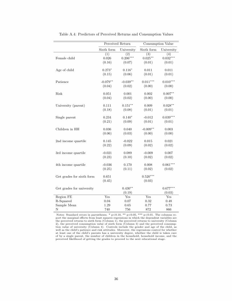
Table A.4: Predictors of Perceived Returns and Consumption Values

Perceived Return Consumption Value

Sixth form University Sixth form University(1) (2) (3) (4)

Female child 0.026 0.206∗∗∗ 0.025∗∗ 0.032∗∗∗

(0.16) (0.07) (0.01) (0.01)

Age of child 0.273∗ 0.116∗ 0.011 0.011(0.15) (0.06) (0.01) (0.01)

Patience -0.079∗∗ -0.039∗∗ 0.011∗∗∗ 0.010∗∗∗

(0.04) (0.02) (0.00) (0.00)

Risk 0.051 0.001 0.002 0.007∗∗

(0.04) (0.02) (0.00) (0.00)

University (parent) 0.111 0.151∗∗ 0.009 0.028∗∗

(0.18) (0.08) (0.01) (0.01)

Single parent 0.234 0.140∗ -0.012 0.039∗∗∗

(0.21) (0.09) (0.01) (0.01)

Children in HH 0.036 0.040 -0.009∗∗ 0.003(0.06) (0.03) (0.00) (0.00)

2nd income quartile 0.145 -0.022 0.015 0.021(0.22) (0.09) (0.02) (0.02)

3rd income quartile -0.021 0.089 -0.009 0.007(0.23) (0.10) (0.02) (0.02)

4th income quartile -0.036 0.170 0.008 0.061∗∗∗

(0.25) (0.11) (0.02) (0.02)

Get grades for sixth form 0.651 0.520∗∗∗

(0.45) (0.03)

Get grades for university 0.430∗∗ 0.677∗∗∗

(0.19) (0.03)Region FE Yes Yes Yes YesR-Squared 0.04 0.07 0.32 0.48Sample Mean 1.29 0.65 0.77 0.73N 740 756 872 866Notes: Standard errors in parentheses. * p<0.10, ** p<0.05, *** p<0.01. The columns re-port the marginal effects from least squares regressions in which the dependent variables arethe perceived returns to sixth form (Column 1), the perceived returns to university (Column2), the perceived consumption value of sixth form (Column 3) and the perceived consump-tion value of university (Column 4). Controls include the gender and age of the child, aswell as the child’s patience and risk attitudes. Moreover, the regressions control for whetherat least one of the child’s parents has a university degree, whether the child is taken careof by a single parent, the number of children in the household, household income, and theperceived likelihood of getting the grades to proceed to the next educational stage.

36

B Questionnaire

1. On a scale of 0-10, where 0 is extremely impatient and 10 is extremely patient, how patient would

you say you are?

2. On a scale of 0-10, where 0 is never and 10 is always, how willing to take risks would you say

you are?

3. How likely (0-100%) do you think it is you will get the grades to stay in full-time education at

the end of year 11?

4. If you get the grades at the end of year 11, how likely (0-100%) do you think it is you will stay

on in full-time education at the end of year 11?

5. If you do stay on after year 11, how likely (0-100%) do you think it is you’ll do well enough in

your future qualifications in sixth form/college to go to university?

6. Assuming you do get the grades in sixth form/college to go to university, how likely do you think

it is that you will go to university?

7. Now look ahead to what you might be doing at the age of 25, and imagine how this might depend

on the education choices you make. How likely do you think it is that you will be in a paid job

when you are 25 if you...

• ... leave full-time education at the end of year 11?

• ... stay in full-time education in sixth form/college but not go to university?

• ... stay in full-time education in sixth form/college and then go to university?

8. If you have a job at the age of 25, what is your best estimate of how much you might be earning

if you...

• ... leave full-time education at the end of year 11?

• ... stay in full-time education in sixth form/college but not go to university?

• ... stay in full-time education in sixth form/college and then go to university?

9. If you do stay on after year 11, how likely (0-100%) do you think it is you would enjoy full-time

education in sixth form/college?

10. If you do go to university, how likely (0-100%) do you think it is that you would enjoy it?

37

C Sample

Figure C.1: Comparison of Household Income Distributions

0.0

5.1

.15

.2

0 £10,000 − £15,999 £30,000 − £34,999 £50,000 − £74,999

Our survey FRS

Note: This figure shows the distribution of annual household income (after tax) for households in our sampleand for a representative sample of households with at least one child aged 12-15 (Source: Family ResourcesSurvey 2013-2014).

38