Embed Size (px)
Citation preview
MONFISPOL Grant no.: 225149
Deliverable 3.1.2
Algorithms for identification analysis under
the DYNARE environment: final version of
software.
Marco Ratto, Joint Research Centre, European Commissionwith the contribution of Nikolai Iskrev, Bank of Portugal
May 30, 2011
Abstract
In this report we document in detail the Identification package de-
veloped for the DYNARE environment. The package implements
methodologies and collects developed algorithms to assess identifica-
tion of DSGE models in the entire prior space of model deep param-
eters, by combining ‘classical’ local identification methodologies and
global tools for model analysis, like global sensitivity analysis.
1

1 Executive summary
In developing the identification software, we took into consideration the most
recent developments in the computational tools for analyzing identification
in DSGE models. A growing interest is being addressed to identification
issues in economic modeling (Canova and Sala, 2009; Komunjer and Ng,
2009; Iskrev, 2010b). The identification toolbox includes the new efficient
method for derivatives computation documented in Deliverable 3.1.1 (JRC,
2010) and presented in Ratto and Iskrev (2010a,b) and the identification
tests proposed by Iskrev.
1.1 Main features of the software
The new DYNARE keyword identification triggers the routines developed
at JRC. This option has two modes of operation.
Point estimate : this is the default option.
• when there is a prior definition for a subset of model parameters
that are going to be estimated, the program performs the local
identification checks for the parameters declared in the prior defi-
nition at the prior mean (prior mode, posterior mean and posterior
mode are also alternative options);
• when there is no prior definition for model parameters, the pro-
gram computes the local identification checks for all the model
parameter values declared in the DYNARE model file. The pa-
rameter values used for identification computations are those de-
2

fined in the model declaration.
Monte Carlo exploration : when information about prior distribution is
provided, a full Monte Carlo analysis is also possible. In this case, for
a number of parameter sets sampled from prior distributions, the local
identification analysis is performed in turn. This provides a ‘global’
prior exploration of local identification properties of DSGE models.
This Monte Carlo mode can also be linked to the the global sensitivity
analysis toolbox, also available in the official DYNARE as of version
4.3.
A library of test routines is also provided in the official DYNARE test
folder. Such tests implement some of the examples described in the present
document.
Kim (2003) : the DYNARE routines for this example are placed in the
folder dynare_root/tests/identification/kim;
An and Schorfheide (2007) : the DYNARE routines for this example are
placed in dynare_root/tests/identification/as2007;
2 DSGE Models
We summarize here briefly the notation of linearized DSGE models and the
restrictions they imply on the first and second order moments of the observed
variables.
3

2.1 Structural model and reduced form
A DSGE model is summarized by a system g of m non-linear equations:
Et
(
g(zt, zt+1, zt−1,ut|θ))
= 0 (1)
where zt is am−dimensional vector of endogenous variables, ut an n-dimensional
random vector of structural shocks with Eut = 0, E utu′
t = In and θ a
k−dimensional vector of deep parameters. Here, θ is a point in Θ ⊂ Rk and
the parameter space Θ is defined as the set of all theoretically admissible
values of θ.
Most studies involving either simulation or estimation of DSGE models
use linear approximations of the original models around the steady-state z∗,
for which g(z∗, z∗, z∗, 0|θ) = 0. Once linearized, most DSGE models can be
written in the following form
Γ0(θ)zt = Γ1(θ) Et zt+1 + Γ2(θ)zt−1 + Γ3(θ)ut (2)
where zt = zt − z∗. The elements of the matrices Γ0, Γ1, Γ2 and Γ3 are
functions of θ.
Depending on the value of θ, there may exist zero, one, or many stable
solutions. Assuming that a unique solution exists, it can be cast in the
following form
zt = A(θ)zt−1 + B(θ)ut (3)
4
where the m×m matrix A and the m× n matrix B are functions of θ.
For a given value of θ, the matrices A, Ω := BB′, and z∗ completely
characterize the equilibrium dynamics and steady state properties of all en-
dogenous variables in the linearized model. Typically, some elements of these
matrices are constant, i.e. independent of θ. For instance, if the steady state
of some variables is zero, the corresponding elements of z∗ will be zero as
well. Furthermore, if there are exogenous autoregressive (AR) shocks in the
model, the matrix A will have rows composed of zeros and the AR coeffi-
cients. As a practical matter, it is useful to separate the solution parameters
that depend on θ from those that do not. We will use τ to denote the vector
collecting the non-constant elements of z∗ , A, and Ω, i.e. τ := [τ ′
z, τ ′
A, τ ′
Ω]′,
where τz, τA, and τΩ denote the elements of z∗, vec(A) and vech(Ω) that
depend on θ.
In some cases, ‘trivial’ singularities in the model dependency w.r.t. θ can
directly tracked in the structural form (2), so we will also use γ to denote
the vector collecting the non-constant elements of Γ0, Γ1, Γ2 and Γ3, i.e.
γ := [γ ′
Γ0, . . . , γ ′
Γ3]′, where γΓi
denote the elements of Γi that depend on θ.
In most applications the model in (3) cannot be taken to the data directly
since some of the variables in zt are not observed. Instead, the solution of
the DSGE model is expressed in a state space form, with transition equation
given by (3), and a measurement equation
xt = Czt + Dut + νt (4)
where xt is a l-dimensional vector of observed variables and νt is a l-dimensional
5

random vector with E νt = 0, Eνtν′
t = Q, where Q is l× l symmetric semi-
positive definite matrix 1.
In the absence of a structural model it would, in general, be impossible to
fully recover the properties of zt from observing only xt. Having the model
in (2) makes this possible by imposing restrictions, through (3) and (4),
on the joint probability distribution of the observables. The model-implied
restrictions on the first and second order moments of the xt are discussed
next.
2.2 Theoretical first and second moments
From (3)-(4) it follows that the unconditional first and second moments of
xt are given by
E xt := µx = s (5)
cov(xt+i,x′
t) := Σx(i) =
CΣz(0)C ′ if i = 0
CAiΣz(0)C ′ if i > 0(6)
where Σz(0) := E ztz′
t solves the matrix equation
Σz(0) = AΣz(0)A′ + Ω (7)
1In the DYNARE framework, the state-space and measurement equations are alwaysformulated such that D = 0
6
Denote the observed data with XT := [x′
1, . . . ,x′
T ]′, and let ΣT be its co-
variance matrix, i.e.
ΣT := E XT X ′
T
=
Σx(0), Σx(1)′, . . . , Σx(T − 1)′
Σx(1), Σx(0), . . . , Σx(T − 2)′
. . . . . . . . . . . .
Σx(T − 1), Σx(T − 2), . . . , Σx(0)
(8)
Let σT be a vector collecting the unique elements of ΣT , i.e.
σT := [vech(Σx(0))′, vec(Σx(1))′, ..., vec(Σx(T − 1))′]′
Furthermore, let mT := [µ′,σ′
T ]′ be a (T−1)l2+l(l+3)/2-dimensional vector
collecting the parameters that determine the first two moments of the data.
Assuming that the linearized DSGE model is determined everywhere in Θ,
i.e. τ is unique for each admissible value of θ, it follows that mT is a function
of θ. If either ut is Gaussian, or there are no distributional assumptions
about the structural shocks, the model-implied restrictions on mT contain
all information that can be used for the estimation of θ. The identifiability
of θ depends on whether that information is sufficient or not. This is the
subject of the next section, where the main results and identification criteria
of Iskrev are summarized.
7

3 Identification
This section recalls the role of the Jacobian matrix of the mapping from θ
to mT for identification, as discussed in Iskrev (2010b), and summarizes the
main computational results concerning its analytic derivation.
3.1 The rank condition
In most applications the distribution of X is unknown or assumed to be
Gaussian. Thus, the estimation of θ is usually based on the first two moments
of the data. If the data is not normally distributed, higher-order moments
may provide additional information about θ, not contained in the first two
moments. Therefore, identification based on the mean and the variance of
X is only sufficient but not necessary for identification with the complete
distribution. In general, there are no known global conditions for unique
solutions of systems of non-linear equations, and it is therefore difficult to
establish the global identifiability of θ. Local identification, on the other
hand, can be verified with the help of the following condition
Theorem 1. Suppose that mT is a continuously differentiable function of θ.
Then θ0 is locally identifiable if the Jacobian matrix J(q) :=∂mq
∂θ′has a full
column rank at θ0 for q ≤ T . This condition is both necessary and sufficient
when q = T if ut is normally distributed.
Note that, J(T ) having full rank is necessary for identification from the
first and second order moments. Therefore, when the rank of J(T ) is less
than k, θ0 is said to be unidentifiable from a model that utilizes only the
8

mean and the variance of XT . A necessary condition for identification in that
sense is that the number of deep parameters does not exceed the dimension
of mT , i.e. k ≤ (T − 1)l2 + l(l + 3)/2.
The local identifiability of a point θ0 can be established by verifying
that the Jacobian matrix J(T ) has full column rank when evaluated at θ0.
Local identification at one point in Θ, however, does not guarantee that the
model is locally identified everywhere in the parameter space. There may be
some points where the model is locally identified, and others where it is not.
Moreover, local identifiability everywhere in Θ is necessary but not sufficient
to ensure global identification. Nevertheless, it is important to know if a
model is locally identified or not for the following two reasons. First, local
identification makes possible the consistent estimation of θ, and is sufficient
for the estimator to have the usual asymptotic properties (see Florens et al.
(2008)). Second, and perhaps more important in the context of DSGE models
is that with the help of the Jacobian matrix we can detect problems that are
a common cause for identification failures in these models. If, for instance,
a deep parameter θj does not affect the solution of the model, it will be
unidentifiable since its value is irrelevant for the statistical properties of the
data generated by the model, and the first and second moments in particular.
Consequently, ∂mT
∂θj- the column of J(T ) corresponding to θj , will be a vector
of zeros for any T , and the rank condition for identification will fail. Another
type of identification failure occurs when two or more parameters enter in the
solution in a manner which makes them indistinguishable, e.g. as a product or
a ratio. As a result it will be impossible to identify the parameters separately,
and some of the columns of the Jacobian matrix will be linearly dependent.
9

An example of the first problem is the unidentifiability of the Taylor rule
coefficients in a simple New Keynesian model pointed out in Cochrane (2007).
An example of the second is the equivalence between the intertemporal and
multisectoral investment adjustment cost parameters in Kim (2003). In these
papers the problems are discovered by solving the models explicitly in terms
of the deep parameters. That approach, however, is not feasible for larger
models, which can only be solved numerically. However, the Jacobian matrix
in Theorem 1 is straightforward to compute analytically for linearized models
of any size or complexity, as shown in (Iskrev, 2010b) and in Ratto and Iskrev
(2010a,b).
3.2 Computing the Jacobian matrix
The simplest method for computing the Jacobian matrix of the mapping from
θ to mT is by numerical differentiation. The problem with this approach is
that numerical derivatives tend to be inaccurate for highly non-linear func-
tions. In the present context this may lead to wrong conclusions concerning
the rank of the Jacobian matrix and the identifiability of the parameters in
the model. For this reason, Iskrev (2010b) applied analytical derivatives, em-
ploying implicit derivation. As shown in Iskrev (2010b), it helps to consider
the mapping from θ to mT as comprising two steps: (1) a transformation
from θ to τ ; (2) a transformation from τ to mT . Thus, the Jacobian matrix
can be expressed as
J(T ) =∂mT
∂τ ′
∂τ
∂θ′(9)
10
The derivation of the first term on the right-hand side is straightforward since
the function mapping τ into mT is available explicitly (see the definition of
τ and equations (5)-(7)); thus the Jacobian matrix J1(T ) := ∂mT
∂τ ′may be
obtained by direct differentiation.
The elements of the second term J2(T ) := ∂τ∂θ′
, the Jacobian of the trans-
formation from θ to τ , can be divided into three groups corresponding to the
three blocks of τ : τz, τA and τΩ. In order to properly compute the deriva-
tives of τA and τΩ, the structural form (2) has to be re-written explicitly
accounting for the dependency to z∗:
Γ0(θ, z∗)zt = Γ1(θ, z
∗) Et zt+1 + Γ2(θ, z∗)zt−1 + Γ3(θ, z
∗)ut (10)
Taking advantage of the DYNARE symbolic pre-processor and after some
implicit derivation steps, discussed in JRC (2010) and Ratto and Iskrev
(2010a,b), all the derivatives information of the structural form (10) can
be obtained.
The derivatives of τA and τΩ can be obtained from the derivatives of
vec(A) and vech(Ω), by removing the zeros corresponding to the constant
elements of A and Ω. In Iskrev (2010b) the derivative of vec(A) is computed
using the implicit function theorem. Such a derivation requires the use of
Kronecker products, implying a dramatic growth in memory allocation re-
quirements and in computational time as the size of the model increases. The
typical size of matrices to be handled in Iskrev (2010b) is of m2 ×m2, which
grows very rapidly with m. Here we apply the alternative method discussed
in Ratto and Iskrev (2010a,b), which allows to reduce both memory require-
11

ments and the computational time, where it is shown that the derivation
problem can be cast in the form of a generalized Sylvester equation and can
be solved using available algebraic solvers. In practice the single big algebraic
problem of dimension m2 × m2 of Iskrev (2010b) is replaced by a set of k
problems of dimension m × m. This allows a significant gain in computa-
tional time of the Sylvester equation solution with respect to the approach
in Iskrev (2010b), making the evaluation of analytic derivatives affordable
also for DSGE models of medium/large scale, enabling to perform detailed
identification analysis for such kind of models.
4 Analyzing local identification of DSGE mod-
els: DYNARE implementation
We have discussed in Section 3 the main Theorem 1 for local identification
of DSGE models as demonstrated by Iskrev (2010b). We need to recall here
another necessary condition discussed in Iskrev (2010b):
Corollary 1. The point θ0 is locally identifiable only if the rank of J2 = ∂τ∂θ′
at θ0 is equal to k.
The condition is necessary because the distribution of XT depends on θ
only through τ , irrespectively of the distribution of ut. It is not sufficient
since, unless all state variables are observed, τ may be unidentifiable.
12
4.1 Identification analysis procedure
The local identifiability of the parameter set θ is established using the nec-
essary and sufficient conditions discussed by Iskrev (2010b):
• Finding that matrix J2 is rank deficient at θ implies that this particular
point in Θ is unidentifiable in the model.
• Finding that J2 has full rank but J(T ) does not, means that θ cannot
be identified given the set of observed variables and the number of
observations.
• On the other hand, if θ is identified at all, it would typically suffice to
check the rank condition for a small number of moments, since J(q)
is likely to have full rank for q much smaller than T . According to
Theorem 1 this is sufficient for identification; moreover, the smaller
matrix may be much easier to evaluate than the Jacobian matrix for
all available moments. A good candidate to try first is the smallest q
for which the order condition is satisfied, and then increase the number
of moments if the rank condition fails;
• the present DYNARE implementation also analyzes the derivatives of
the LRE form of the model (JΓ = ∂γ
∂θ′), to check for ‘trivial’ non-
identification problem, like two parameters always entering as a product
in Γi matrices;
• whenever some of the matrices J2, J(T ) or JΓ is rank deficient, the
code tries to diagnose the subset of parameters responsible for the rank
deficiency: this is done by doing a number of tests
13

1. if there are columns of zeros in the J(·) matrix, the associated
parameter is printed on the MATLAB command window;
2. compute pairwise- and multi-correlation coefficients for each col-
umn of the J(·) matrix: if there are parameters with correlation
coefficients equal to unity, these are printed on the MATLAB com-
mand window;
3. take the Singular Values Decomposition (SVD) of J(·) and track
the eigenvectors associated to the zero singular values.
4.2 Identification strength
The previous conditions are related to whether of not columns of J(T ) or J2
are linearly dependent. Another typical avenue in DSGE models is weak iden-
tification: in this case it is interesting to rank model parameters in terms of
strength of identification. A measure of identification strength is introduced,
following the work of Iskrev (2010a) and Andrle (2010). This can be based on
either using the asymptotic information matrix or using simulated moments
uncertainty mapped onto the deep parameters.
Asymptotic Information Matrix. Given a sample size T , the Fischer in-
formation matrix IT (θ) is computed as discussed in Iskrev (2010a).
Simulated moments. The uncertainty of simulated moments is evalu-
ated, by performing stochastic simulations for T periods and com-
puting sample moments of observed variables; this is repeated for Nr
replicas, giving a sample of dimension Nr of simulated moments; from
14

this the covariance matrix Σ(mT ) of (first and second) simulated mo-
ments is obtained. A ‘moment information matrix’ can be defined as
IT (θ|mT ) = J ′
2 · Σ(mT ) · J2;
The procedure implemented in DYNARE takes the following steps:
1. given the information matrix (either the true one or the one based on
simulated moments), the strength of identification for parameter θi is
defined as
si =√
θ2i /(IT (θ)−1)(i,i) (11)
which is a sort of a priori ‘t-test’ for θi;
2. as discussed in Iskrev (2010a), this measure is made of two compo-
nents: the ‘sensitivity’ and the ‘correlation’, i.e. weak identification
may be due to the fact that moments do not change with θi or or that
other parameters can compensate linearly the effect of θi; the sensitivity
component is defined as
∆i =√
θ2i · IT (θ)(i,i) (12)
3. as an alternative option to ‘normalize’ the identification strength mea-
sures, in place of using θi, the toolbox also uses the value for its prior
standard deviation σ(θi), i.e.:
spriori = σ(θi)/
√
(IT (θ)−1)(i,i)
∆priori = σ(θi) ·
√
IT (θ)(i,i)
15

this normalization for the identification strength weights the informa-
tion derived from the likelihood using the prior uncertainty; this is
specially useful to distinguish those cases where (11) is singular simply
because θi ≈ 0 (e.g. for parameters whose prior distribution is centered
in zero) and therefore θi should NOT be flagged as non- (or weakly)
identified.
The default of the identification toolbox is to show, after the check of rank
conditions, the plots of the strength of identification and of the sensitivity
component for all estimated parameters.
4.3 Analyzing identification patterns
Identification patterns are essentially tracked in two ways:
1. As suggested by Andrle (2010), the identification patterns are shown
by taking the singular value decomposition of IT (θ) or of the J(q)
matrix and displaying the eigenvectors corresponding to the smallest
(or highest) singular values;
2. As discussed in Iskrev (2010b), it is also interesting to check which
group of one, two or more parameters is most capable to mimic (replace)
the effect of each parameter; in other words, a brute force search is done
for each column of J(q)(j) to detect the group of columns J(q)(I+j),
indexed by I, that has the highest explanatory power for J(q)(j) by a
linear regression.
In this analysis, scaling issues in the Jacobian can matter in interpret-
ing results. In medium-large scale DSGE models there can be as many as
16

thousands entries in J(q) and J2 matrices (as well as in corresponding mq
and τ matrices). Each row of J(q) and J2 correspond to a specific moment
or τ element and there can be differences by orders of magnitude between
the values in different rows. In this case, the analysis would be dominated
by the few rows with large elements, while it would be unaffected by all re-
maining elements. This can imply loss of ‘resolution’. Iskrev (2010b) used
the elasticities, so that the (j, i) element of the Jacobian is∂mj
∂θi
θi
mj. This give
the percentage change in the moment for 1% change in the parameter value.
Here we re-scale each row of J(q) and J2 by its largest element in absolute
value. In other words, assuming J2 made of the two rows:
0.1 −0.5 2.5
−900 500 200
multi-collinearity analysis will be performed on the scaled matrix:
0.04 −0.2 1
−1 0.5556 0.2222
The effect of this scaling is that the order of magnitude of derivatives of
any moment (or any τ element) is the same. In other words, this grossly
corresponds to an assumption that the model is equally informative about
moments, thus implying equal weights across different rows of the Jacobian
matrix.
17

4.4 The optional Monte Carlo implementation
This optional implementation is based on Monte Carlo exploration of the
space Θ of model parameters. In particular, a sample from Θ is made of
many randomly drawn points from Θ′, where Θ ∈ Θ′ discarding values of θ
that do not imply a unique solution. The set Θ′ contains all values of θ that
are theoretically plausible, and may be constructed by specifying a lower
and an upper bound for each element of θ or by directly specifying prior
distributions. After specifying a distribution for θ with support on Θ′, one
can obtain points from Θ by drawing from Θ′ and removing draws for which
the model is either indetermined or does not have a solution. Conditions
for existence and uniqueness are automatically checked by DYNARE. The
checks for local identification are then performed for each parameter set in
turn, obtaining a Monte Carlo sample of identification features for the model
under analysis.
4.4.1 Sensitivity measures
The identification analysis is linked to the idea of sensitivity analysis, where
the analyst would like to track how model ‘outputs’ (in this case τ or mT
or the likelihood itself) are affected by changes in θ. In a context where
plausible parameter ranges are wide and the associated model features can
significantly change in such a wide domain, global sensitivity analysis (GSA)
provides useful diagnostic tools to measures that importance of the various
parameters. The GSA, the reference measures are the variance-based sensi-
tivity indices (Ratto, 2008).
18
Let Y be a generic ‘output’ of the model: in this case τ or mT elements.
Given the model structure, the outcome of Y depends on the values of θ. This
dependence can be expressed as a non linear relationship Y = f(θ1, . . . , θk),
whose analytic form is unknown to the analyst. Such a relationship can be
represented by mean of ANOVA (or ANOVA-HDMR) decompositions, where
ANOVA stands for ‘analysis of variance’, the ensemble the statistical tools
for in which the observed variance in a particular variable Y is partitioned
into components attributable to different sources of variation and HDMR
stands for High-Dimensional Model representation (Sobol’, 1990; Gu, 2002).
In ANOVA, the function f is decomposed by means of a finite decomposition
into terms of increasing dimensionality:
f(θ1, θ2, . . . , θk) = f0 +∑
i
fi +∑
i
∑
j>i
fij + . . .+ f12...k (13)
where each term is a function only of the parameters in its indexes, i.e.
fi = f(θi), fij = f(θi, θj) and so on. The various terms are expressed as:
f0 = E(Y )
fi(θi) = E(Y |θi) − f0 (14)
fij = E(Y |θi, θj) − f(θi) − f(θj) − f0
If θ values are sampled independently, all the terms of the decomposition
are orthogonal and the decomposition (13) is unique. The f ′
is are called the
main effects, f ′
ijs are the second order interaction effects, and so on. Each
term of the decomposition tells the analyst how much Y moves around its
19

mean level f0 as a function of each of the input factors or group of them.
An intuitive way to derive a scalar measure of the importance of θi on the
variation of Y , is to take the variance V (fi) = Vi and compare it to the total
variance V (Y ). Normalizing the partial variances with the unconditional
variance V = V (Y ), the sensitivity indices are obtained: Si = Vi/V (main
effects) , Sij = Vij/V (second order pure interaction effects), etc. Variance
based sensitivity indices provide the percentage of output model variance
which is explained by each input.
Various approaches for estimating variance based sensitivity indices are
available. These may require either the use of specific sampling strategies to
directly estimate sensitivity indices (Sobol’, 1990; Saltelli et al., 2010) or by
estimating some ‘metamodel’ using a Monte Carlo sample of the mapping f
and deriving sensitivity indices from the metamodel (Oakley and O’Hagan,
2004; Storlie and Helton, 2007; Ratto and Pagano, 2010). In the present
context, running such kind of sophisticated estimators may imply either too
many runs of the model solutions than affordable (specially for medium-large
scale models) or to repeat computer intensive metamodelling estimations for
the large number of ‘outputs’ under consideration (in particular the mT
elements).
For the purpose of the identification toolbox it is sufficient to take an
approximation of the full variance based approach which allows to synthesize
effectively the information coming from the Jacobian J(q). The Jacobian
(i.e. local derivatives) provide per se ‘local’ sensitivity measures and in fact
this has been historically the first approach to sensitivity analysis. It is
also well known that derivative based sensitivity poses some problems of
20

interpretation, due to scaling issues and to the fact that derivatives may not
be directly comparable to each others and also due to the fact they only
reflect the local behavior of the mapping f possibly leading to erroneous
results. So, first, the derivatives are usually normalized if they ought to be
used for sensitivity purposes: Iskrev (2010b) uses elasticities, implying that
the new sensitivity measure gives the percentage change in the moment for 1%
change in the parameter value. This somehow improves the interpretability
of the measure, but still carries in some issues relative to the specific point
where the derivatives are taken: for example what if derivatives are taken
at a location where θj = 0 or Y = 0? Moreover, no information about the
degree of uncertainty about each parameters comes in in such a sensitivity
measure. Therefore, in order to link derivatives to the reference variance-
based measure, it is most advisable to proceed as follows.
Derivatives provide a local approximation of the mapping f around the
specific sample point θ(j) where derivatives are taken:
f(θ) ≈ Y (θ(j)) + J(θ(j)) · (θ − θ(j)) (15)
and the variance based sensitivity indices for this linearized mapping simply
read (assuming independent θ’s):
Si ≈
(
∂Y
∂θi
)2
(j)
· V (θi)/V (Y ) (16)
where V (θi) is the prior variance of each parameter and V (Y ) is the variance
of the model ‘output’ (i.e. mT elements). This approach to scaling deriva-
21

tives links the local sensitivity to two key global elements: the ‘uncertainty’
about the parameters and the ‘uncertainty’ about the outputs. This mea-
sure provides the portion of the linearized mapping f that is explained by
each parameter. This implies that, if Y has the same derivative w.r.t. two
parameters, the most ‘important’ parameter will be the one with the highest
uncertainty (i.e. variance), since it will be responsible for higher changes in
the output value. With the Monte Carlo exploration of the parameter space,
one will have the availability of these sensitivity measures for each element
of the sample: taking the average of these measures provides a synthetic
measure of sensitivity measure that averages the local effect over the entire
prior space.
To summarize, the program performs the following steps to compute sen-
sitivity measures of theoretical moments with respect to model parameters:
1. given the MC sample of θ, the sample for mT is stored, allowing to
compute the sample variance for each of their elements V (mj);
2. all computed derivatives are normalized, so that the (j, i) element of
the Jacobian is∂mj
∂θi
std(θi)std(mj )
;
3. for each MC sample point we take the norm of the normalized Jacobian,
obtaining one single aggregate sensitivity measure for each parameter
and each sample point;
4. this aggregate measure is finally averaged over the MC sample, provid-
ing the final sensitivity measure reported by the identification toolbox.
In the case of the point estimate (the default case), no direct information
22

about the variances V (mj) is available. Hence, given the covariance Σθ of
the parameters, the variance of the moments is obtained as J(q) · Σθ · J(q)′.
5 DYNARE syntax
A new syntax is made available for DYNARE users. The simple keyword
identification(<options>=<values>); triggers the point identification
analysis, performed at the prior mean. Prior definitions and the list of ob-
served values are needed, using the standard DYNARE syntax for setting-up
an estimation.
Current options are as follows (all options will be discussed in detail in
the Examples section 6):
• parameter set = prior mode | prior mean | posterior mode | posterior mean
| posterior median. Specify the parameter set to use. Default: prior_mean.
• prior_mc = INTEGER sets the number of Monte Carlo draws (default
= 1); prior_mc=1 triggers the default point identification analysis;
prior_mc>1 triggers the Monte Carlo mode;
• prior_range = INTEGER triggers uniform sample within the range im-
plied by the prior specifications (when prior_mc>1). Default: 0
• load_ident_files = 0, triggers a new analysis, while load_ident_files = 1,
loads and displays a previously performed analysis (default = 0);
• ar = <integer> (default = 3), triggers the value for q in computing
J(q);
23
• useautocorr: this option triggers J(q) in the form of auto-covariances
and cross-covariances (useautocorr = 0), or in the form of auto-correlations
and cross-correlations (useautocorr = 1). The latter form normalizes
all mq entries in [−1, 1] (default = 0).
• advanced = INTEGER triggers standard or advanced identification anal-
ysis (default = 0). In standard identification analysis the rank con-
dition is checked and, if it fails, indicates the parameter(s) that are
not identified; the strength of identification plus the sensitivity com-
ponent is also provided. The advanced identification analysis shows
a more detailed analysis, comprised of an analysis for the linearized
rational expectation model as well as the associated reduced form so-
lution. Moreover, a detailed information about identification patterns
is also provided, as discussed in Section 4.3. In the collinearity analy-
sis by brute force search of the groups of parameters best reproducing
the behavior of each single parameter (Iskrev, 2010b), the maximum
dimension of the group searched is triggered by max_dim_cova_group.
In the Monte Carlo mode, the advanced options triggers a number of
additional diagnostics: (i) analysis of the condition number of the Ja-
cobians J(q), J2 and JΓ and detection of the parameters that mostly
drive large condition numbers (i.e. weaker identification); (ii) analysis
of the identification patters across the Monte Carlo sample; (iii) de-
tailed point-estimate (identification strength and collinearity analysis)
of the parameters set having the smallest/largest condition number;
(iv) when some singularity (rank condition failure) is detected for some
24

elements of the Monte Carlo sample, detailed point-estimates are per-
formed for such critical points.
• max_dim_cova_group = INTEGER In the brute force search (performed
when advanced=1) this option sets the maximum dimension of groups
of parameters that best reproduce the behavior of each single model
parameter. Default: 2
• periods = INTEGER triggers the length of the stochastic simulation to
compute the analytic Hessian. Default: 300
• periods = INTEGER When the analytic Hessian is not available (i.e.
with missing values or diffuse Kalman filter or univariate Kalman filter),
this triggers the length of stochastic simulation to compute Simulated
Moments Uncertainty. Default: 300
• replic = INTEGER When the analytic Hessian is not available, this
triggers the number of replicas to compute Simulated Moments Uncer-
tainty. Default: 100.
• gsa_sample_file = INTEGER If equal to 0, do not use sample file. If
equal to 1, triggers GSA prior sample. If equal to 2, triggers GSA
Monte-Carlo sample (i.e. loads a sample corresponding to pprior=0
and ppost=0 in the dynare_sensitivity options). Default: 0
• gsa_sample_file = FILENAME Uses the provided path to a specific
user defined sample file. Default: 0
25
6 Examples
6.1 Kim (2003)
In this paper, Kim demonstrated a functional equivalence between two types
of adjustment cost specifications, coexisting in macroeconomic models with
investment: intertemporal adjustment costs which involve a nonlinear sub-
stitution between capital and investment in capital accumulation, and mul-
tisectoral costs which are captured by a nonlinear transformation between
consumption and investment. We reproduce results of Kim (2003), worked
out analytically, applying the DYNARE procedure on the non-linear form of
the model. The representative agent maximizes
∞∑
t=0
βt logCt (17)
subject to a national income identity and a capital accumulation equation:
(1 − s)( Ct
1 − s
)1+θ
+ s(Its
)1+θ
= (AtKαt )1+θ (18)
Kt+1 =
[
δ
(
Itδ
)1−φ
+ (1 − δ)K1−φt
]1
1−φ
(19)
where s = βδα∆
, ∆ = 1 − β + βδ, φ(≥ 0) is the inverse of the elasticity
of substitution between It and Kt and θ(≥ 0) is the inverse of the elastic-
ity of transformation between consumption and investment. Parameter φ
represents the size of intertemporal adjustment costs while θ is called the
multisectoral adjustment cost parameter. Kim shows that in the linearized
form of the model, the two adjustment cost parameter only enter through an
26
‘overall’ adjustment cost parameter Φ = φ+θ1+θ
, thus implying that they cannot
be identified separately.
Here we assume that the Kim model is not analytically worked out to
highlight this problem of identification. Instead, the analyst feeds the non-
linear model (constraints and Euler equation) to DYNARE (also note that
the adjustment costs are defined in such a way that the steady state is not
affected by them).
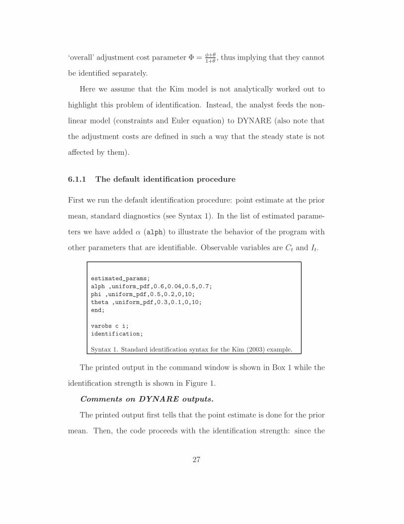
6.1.1 The default identification procedure
First we run the default identification procedure: point estimate at the prior
mean, standard diagnostics (see Syntax 1). In the list of estimated parame-
ters we have added α (alph) to illustrate the behavior of the program with
other parameters that are identifiable. Observable variables are Ct and It.
estimated_params;
alph ,uniform_pdf,0.6,0.04,0.5,0.7;
phi ,uniform_pdf,0.5,0.2,0,10;
theta ,uniform_pdf,0.3,0.1,0,10;
end;
varobs c i;
identification;
Syntax 1. Standard identification syntax for the Kim (2003) example.
The printed output in the command window is shown in Box 1 while the
identification strength is shown in Figure 1.
Comments on DYNARE outputs.
The printed output first tells that the point estimate is done for the prior
mean. Then, the code proceeds with the identification strength: since the
27

==== Identification analysis ====
Testing prior mean
Evaluting simulated moment uncertainty ... please wait
Doing 100 replicas of length 300 periods.
Simulated moment uncertainty ... done!
WARNING !!!
The rank of H (model) is deficient!
[theta,phi] are PAIRWISE collinear (with tol = 1.e-10) !
WARNING !!!
The rank of J (moments) is deficient!
[theta,phi] are PAIRWISE collinear (with tol = 1.e-10) !
==== Identification analysis completed ====
Box 1. Standard printed output for the Kim (2003) example.
model has two observables and only one shock (technology) the Kalman filter
is rank deficient and the analytic asymptotic Hessian cannot be computed.
Hence, the alternate procedure based on simulated moments uncertainty is
applied. The rank condition fails for both for J2 (called H in the DYNARE
output) and J(q), implying that sufficient and necessary conditions for local
identification are not fulfilled by this model. Moreover, perfect collinearity
among columns for θ and φ is detected both for J2 and J(q), thus allowing
to highlight which combination of parameters is responsible for the lack of
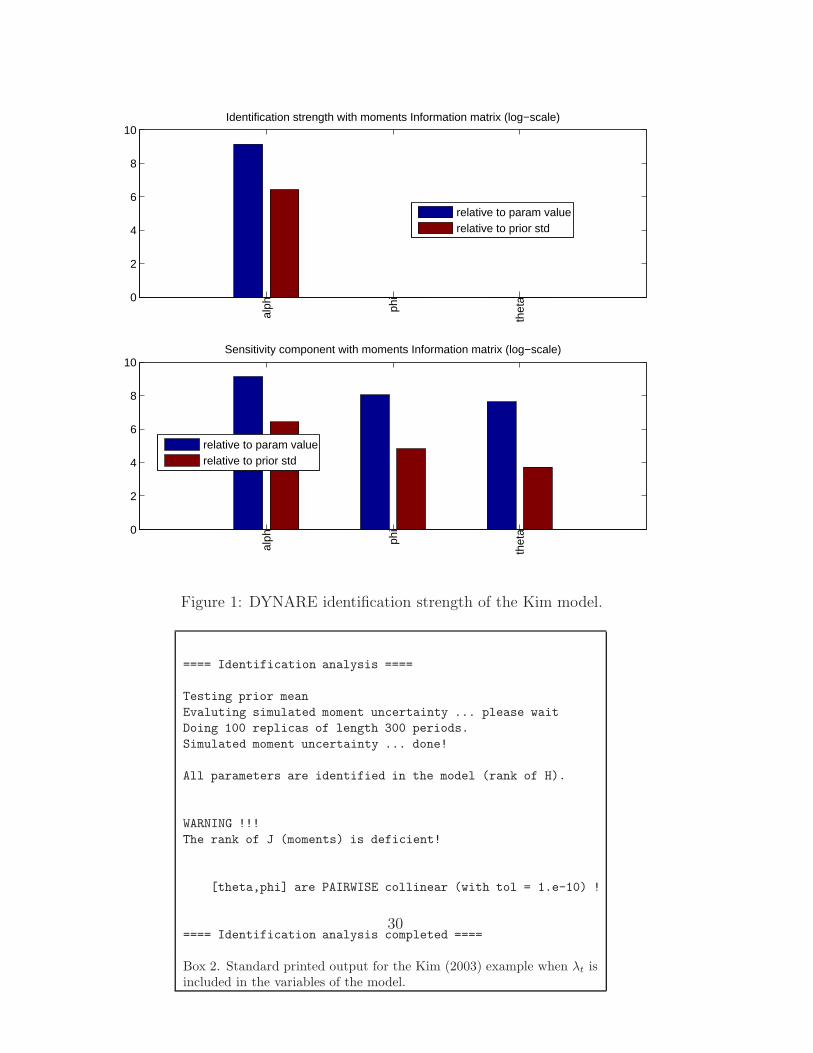
identification. The plot of the strength of identification (Figure 1) tells that
α is identified while identification strength for θ and φ is null (in practice
28

no bar is shown in the log-scale plot). It is interesting to look at the sen-
sitivity component for the three parameters, which tells that all parameters
have individually an effect on the model behavior, implying that it is indeed
the correlation component that drives the rank-deficiency. The strength of
identification plot is saved in the identification subfolder with the name
MODEL_ident_strength. So, the diagnostic tests implemented in DYNARE
perfectly reveal the identification problem demonstrated analytically by Kim.
This result shows that the procedures implemented in DYNARE can help the
analyst in detecting identification problems in all typical cases where such
problems cannot easily worked out analytically.
It seems also interesting to show here the effect of the number of states
fed to DYNARE on the results of the identification analysis. For simplic-
ity of coding, Lagrange multipliers may be explicitly included in the model
equations. In this case, one would have an additional equation for the La-
grange multiplier λt = (1−s)θ
(1+θ)C(1+θ)t
, with λt entering the Euler equation. The
DYNARE output is shown in Box 2. Under this kind of implementation,
and still assuming that only Ct and It can be observed, the test for J(q) still
the rank deficiency, thus confirming the identification problem. On the other
hand, due to the specific effect of θ on λt, our identification tests would tell
that θ and φ are separably identified in the model, provided that all states
are observed. This exemplifies the nature of the necessary condition stated
in Corollary 1.
29
0
2
4
6
8
10
alph ph
i
thet
a
Identification strength with moments Information matrix (log−scale)
relative to param valuerelative to prior std
0
2
4
6
8
10
alph ph
i
thet
a
Sensitivity component with moments Information matrix (log−scale)
relative to param valuerelative to prior std
Figure 1: DYNARE identification strength of the Kim model.
==== Identification analysis ====
Testing prior mean
Evaluting simulated moment uncertainty ... please wait
Doing 100 replicas of length 300 periods.
Simulated moment uncertainty ... done!
All parameters are identified in the model (rank of H).
WARNING !!!
The rank of J (moments) is deficient!
[theta,phi] are PAIRWISE collinear (with tol = 1.e-10) !
==== Identification analysis completed ====
Box 2. Standard printed output for the Kim (2003) example when λt isincluded in the variables of the model.
30
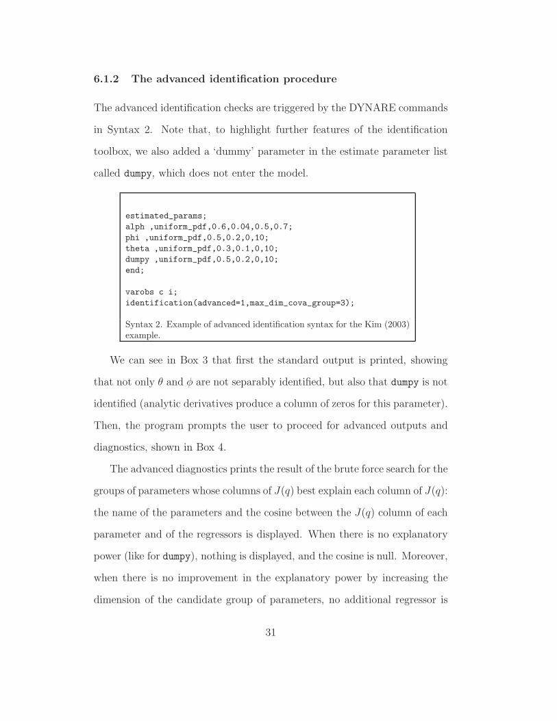
6.1.2 The advanced identification procedure
The advanced identification checks are triggered by the DYNARE commands
in Syntax 2. Note that, to highlight further features of the identification
toolbox, we also added a ‘dummy’ parameter in the estimate parameter list
called dumpy, which does not enter the model.
estimated_params;
alph ,uniform_pdf,0.6,0.04,0.5,0.7;
phi ,uniform_pdf,0.5,0.2,0,10;
theta ,uniform_pdf,0.3,0.1,0,10;
dumpy ,uniform_pdf,0.5,0.2,0,10;
end;
varobs c i;
identification(advanced=1,max_dim_cova_group=3);
Syntax 2. Example of advanced identification syntax for the Kim (2003)example.
We can see in Box 3 that first the standard output is printed, showing
that not only θ and φ are not separably identified, but also that dumpy is not
identified (analytic derivatives produce a column of zeros for this parameter).
Then, the program prompts the user to proceed for advanced outputs and
diagnostics, shown in Box 4.
The advanced diagnostics prints the result of the brute force search for the
groups of parameters whose columns of J(q) best explain each column of J(q):
the name of the parameters and the cosine between the J(q) column of each
parameter and of the regressors is displayed. When there is no explanatory
power (like for dumpy), nothing is displayed, and the cosine is null. Moreover,
when there is no improvement in the explanatory power by increasing the
dimension of the candidate group of parameters, no additional regressor is
31

==== Identification analysis ====
Testing prior mean
Evaluting simulated moment uncertainty ... please wait
Doing 100 replicas of length 300 periods.
Simulated moment uncertainty ... done!
WARNING !!!
The rank of H (model) is deficient!
dumpy is not identified in the model!
[dJ/d(dumpy)=0 for all tau elements in the model solution!]
[theta,phi] are PAIRWISE collinear (with tol = 1.e-10) !
WARNING !!!
The rank of J (moments) is deficient!
dumpy is not identified by J moments!
[dJ/d(dumpy)=0 for all J moments!]
[theta,phi] are PAIRWISE collinear (with tol = 1.e-10) !
Press ENTER to display advanced diagnostics
Box 3. Standard printed output for the Kim (2003) example when dumpy
is included in the prior list for estimation.
32

Collinearity patterns with 1 parameter(s)
Parameter [ Expl. params ] cosn
alph [ theta ] 0.800
phi [ theta ] 1.000
theta [ phi ] 1.000
dumpy [ -- ] 0.000
Collinearity patterns with 2 parameter(s)
Parameter [ Expl. params ] cosn
alph [ phi theta ] 0.975
phi [ theta -- ] 1.000
theta [ phi -- ] 1.000
dumpy [ -- -- ] 0.000
Collinearity patterns with 3 parameter(s)
Parameter [ Expl. params ] cosn
alph [ phi theta -- ] 0.975
phi [ theta -- -- ] 1.000
theta [ phi -- -- ] 1.000
dumpy [ -- -- -- ] 0.000
==== Identification analysis completed ====
Box 4. Advanced printed output for the Kim (2003) example.
added (see printed results for 3 parameters) and the cosine does not improve
with respect to the group of smaller dimensionality.
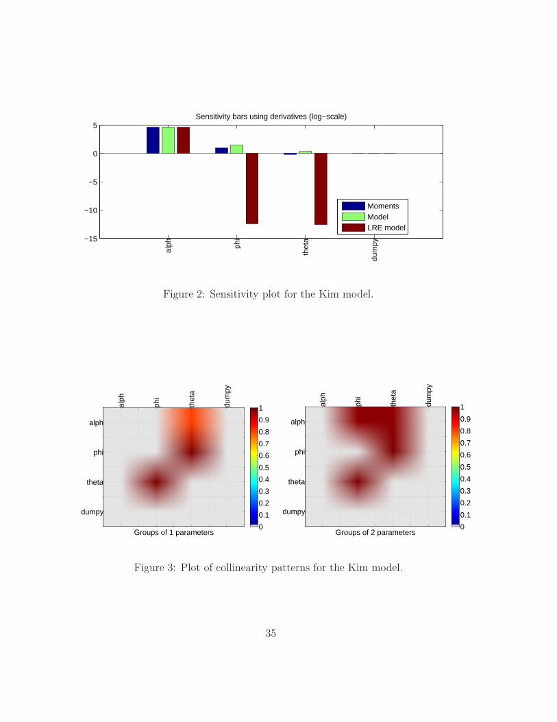
The advanced diagnostics also produces three kinds of additional plots:
the sensitivity plot, the collinearity patterns, the identification patterns a la
Andrle (2010).
Sensitivity plot. This plot shows the sensitivity measures computed as de-
scribed in Section 4.4.1, i.e. the norm of the columns of the jacobian
matrices for the moments (J(q)), the model (J2), the LRE model (JΓ)
normalized by the relative uncertainties in model parameters and out-
put values. An example of this is in Figure 2. This plot is saved in the
33

identification subfolder with the name MODEL_sensitivity.
Collinearity patterns. These plots synthesize the results of the brute force
search a la Iskrev (2010b) already printed in Box 4. Specially for large
models and large number of parameters, these plots allow a quick search
for the critical collinearities (i.e. dark red spots). Examples of these are
shown in Figure 3: the critical combination between θ and φ is clearly
indicated. These plots are saved in the identification subfolder with
the names MODEL_ident_collinearity_*.
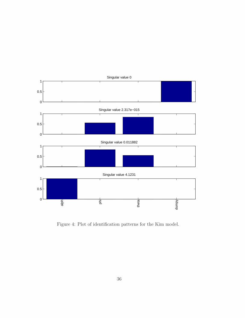
Identification patterns. As suggested by Andrle (2010), identification pat-
terns can be analyzed by taking the singular value decomposition of
the Information Matrix or of the Jacobian. The plots produced by the
identification toolbox show in bar form the eigenvectors relative to the
smallest and largest singular values: the former indicate the parame-
ters that are mostly affected by weak or lack of identification, while
the latter indicate parameters that can be best identified. An example
of this for the Kim model is shown in Figure 4. We can see in this
figure that there are two null singular values, one associated to dumpy,
the other associated to the couple [θ, φ]. Moreover, the positive sin-
gular values are associated with α and [θ, φ], indicating that only the
linear combination of the latter couple of parameters can be identified.
These plots are saved in the identification subfolder with the names
MODEL_ident_pattern_*.
34
−15
−10
−5
0
5
alph ph
i
thet
a
dum
py
Sensitivity bars using derivatives (log−scale)
MomentsModelLRE model
Figure 2: Sensitivity plot for the Kim model.
alph
alph
phi
phi
thet
a
theta
dum
py
dumpy
Groups of 1 parameters
0
0.1
0.2
0.3
0.4
0.5
0.6
0.7
0.8
0.9
1 alph
alph
phi
phi
thet
a
theta
dum
py
dumpy
Groups of 2 parameters
0
0.1
0.2
0.3
0.4
0.5
0.6
0.7
0.8
0.9
1
Figure 3: Plot of collinearity patterns for the Kim model.
35
0
0.5
1Singular value 0
0
0.5
1Singular value 2.317e−015
0
0.5
1Singular value 0.011882
0
0.5
1
alph ph
i
thet
a
dum
pySingular value 4.1231
Figure 4: Plot of identification patterns for the Kim model.
36

6.2 An and Schorfheide (2007)
The model An and Schorfheide (2007), linearized in log-deviations from
steady state, reads:
yt = Et[yt+1] + gt − Et[gt+1] − 1/τ · (Rt −Et[πt+1] − Et[zt+1]) (20)
πt = βEt[πt+1] + κ(yt − gt) (21)
Rt = ρRRt−1 + (1 − ρR)ψ1πt + (1 − ρR)ψ2(∆yt − zt) + εR,t (22)
gt = ρggt−1 + εg,t (23)
zt = ρzzt−1 + εz,t (24)
where yt is GDP in efficiency units, πt is inflation rate, Rt is interest rate,
gt is government consumption and zt is change in technology. The model is
completed with three observation equations for quarterly GDP growth rate
(Y GRt), annualized quarterly inflation rates (INFt) and annualized nominal
interest rates (INTt):
Y GRt = γQ + 100 ∗ (yt − yt−1 + zt) (25)
INFLt = πA + 400πt (26)
INTt = πA + rA + 4γQ + 400Rt (27)
where β = 11+rA/400
.
For this example we will consider and discuss in detail the Monte Carlo
option.
37

6.2.1 Standard Monte Carlo procedure
An example of DYNARE syntax for this is shown in Syntax 3: we perform a
loop of 250 local identification analyzes at parameter values randomly chosen
in the prior distributions.
estimated_params;
tau, gamma_pdf, 2, 0.5;
kap, beta_pdf, 0.2, 0.1;
psi1, gamma_pdf, 1.5, 0.25;
psi2, gamma_pdf, 0.5, 0.25;
rhoR, beta_pdf, 0.5, 0.2;
rhog, beta_pdf, 0.8, 0.1;
rhoz, beta_pdf, 0.66, 0.15;
rr_steady, gamma_pdf, 0.8, 0.5;
pi_steady, gamma_pdf, 0.8, 0.5;
gam_steady, gamma_pdf, 0.8, 0.5;
std_R, inv_gamma_pdf, 0.05, inf;
std_g, inv_gamma_pdf, 0.05, inf;
std_z, inv_gamma_pdf, 0.05, inf;
end;
varobs YGR INFL INT;
identification(prior_mc=250);
Syntax 3. Identification syntax for Monte Carlo identification analysisof the An and Schorfheide (2007) example.
The standard output printed on the command window by the program is
reported in Box 5: the program execution first performs the point estimated
at the prior mean, as in the default execution. Then, it loops over the 250
replicas. The result of the identification analysis indicates that all parameters
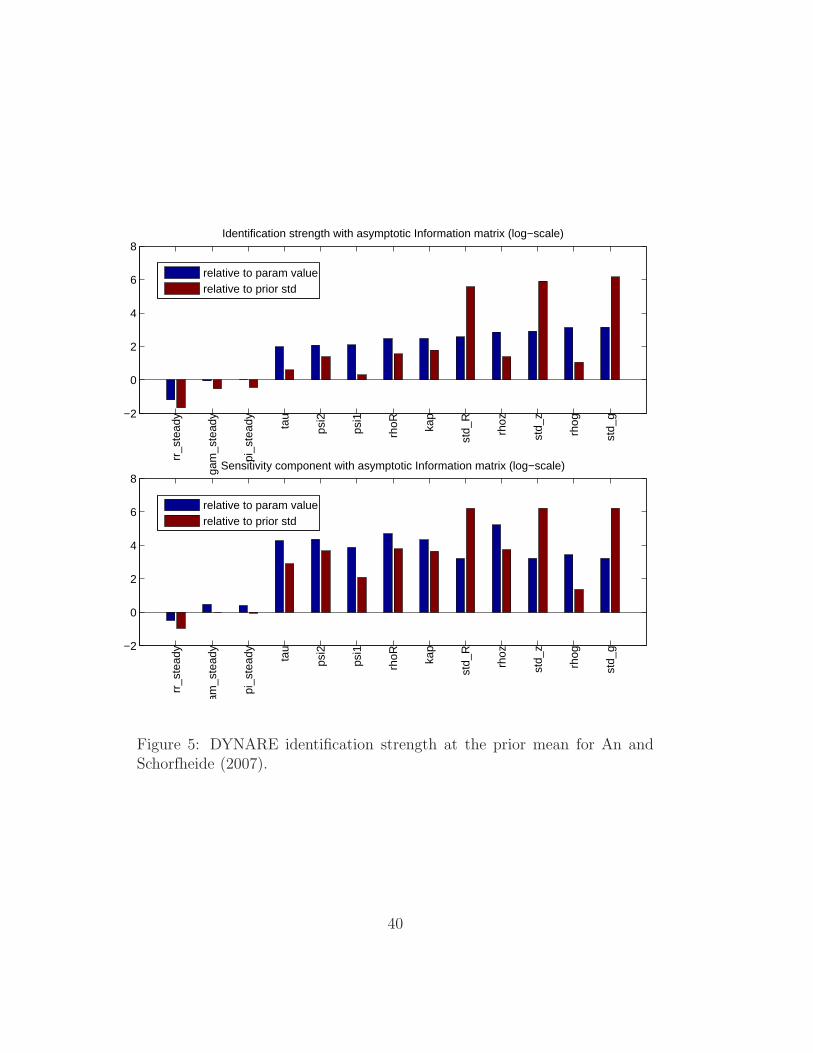
are identified in the model and in the moments in the entire prior space. The
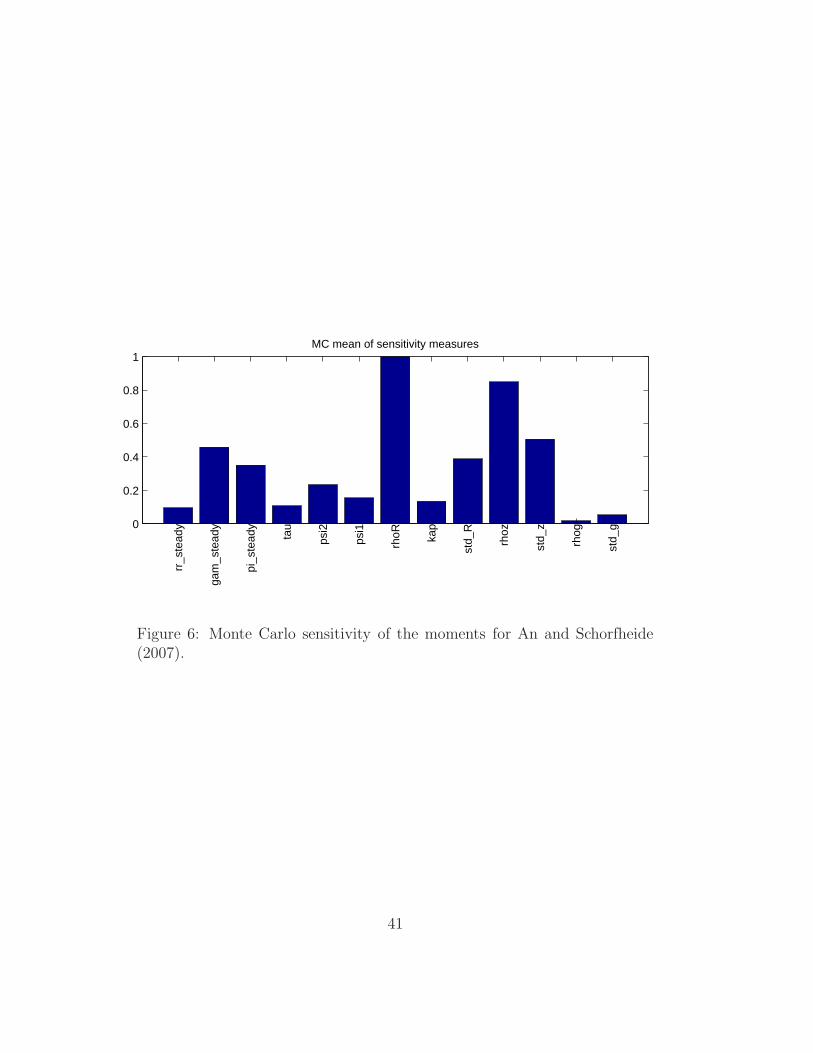
graphical output is made of two plots: first the identification strength at
the prior mean (Figure 5), second the Monte Carlo mean of the sensitivity
measures as described in Section 4.4.1 (Figure 6). In this case, the number
38

==== Identification analysis ====
Testing prior mean
All parameters are identified in the model (rank of H).
All parameters are identified by J moments (rank of J)
Monte Carlo Testing
Testing MC sample
All parameters are identified in the model (rank of H).
All parameters are identified by J moments (rank of J)
==== Identification analysis completed ====
Box 5. Printed output for the An and Schorfheide (2007) example when theMonte Carlo option is triggered.
of shocks equals the number of observables, so the asymptotic Hessian of the
likelihood function can be evaluated for the identification strength. In Figure
5 we can see that all parameters are identified: the model parameters on the
x-axis are ranked in increasing order of strength of identification. In the plot
for the sensitivity analysis component and of the Monte Carlo sensitivity, we
can also see that all parameters have a non-negligible effect on the moments.
39
−2
0
2
4
6
8
rr_s
tead
y
gam
_ste
ady
pi_s
tead
y
tau
psi2
psi1
rhoR ka
p
std_
R
rhoz
std_
z
rhog
std_
g
Identification strength with asymptotic Information matrix (log−scale)
relative to param valuerelative to prior std
−2
0
2
4
6
8
rr_s
tead
y
gam
_ste
ady
pi_s
tead
y
tau
psi2
psi1
rhoR ka
p
std_
R
rhoz
std_
z
rhog
std_
g
Sensitivity component with asymptotic Information matrix (log−scale)
relative to param valuerelative to prior std
Figure 5: DYNARE identification strength at the prior mean for An andSchorfheide (2007).
40
0
0.2
0.4
0.6
0.8
1
rr_s
tead
y
gam
_ste
ady
pi_s
tead
y
tau
psi2
psi1
rhoR ka
p
std_
R
rhoz
std_
z
rhog
std_
g
MC mean of sensitivity measures
Figure 6: Monte Carlo sensitivity of the moments for An and Schorfheide(2007).
41

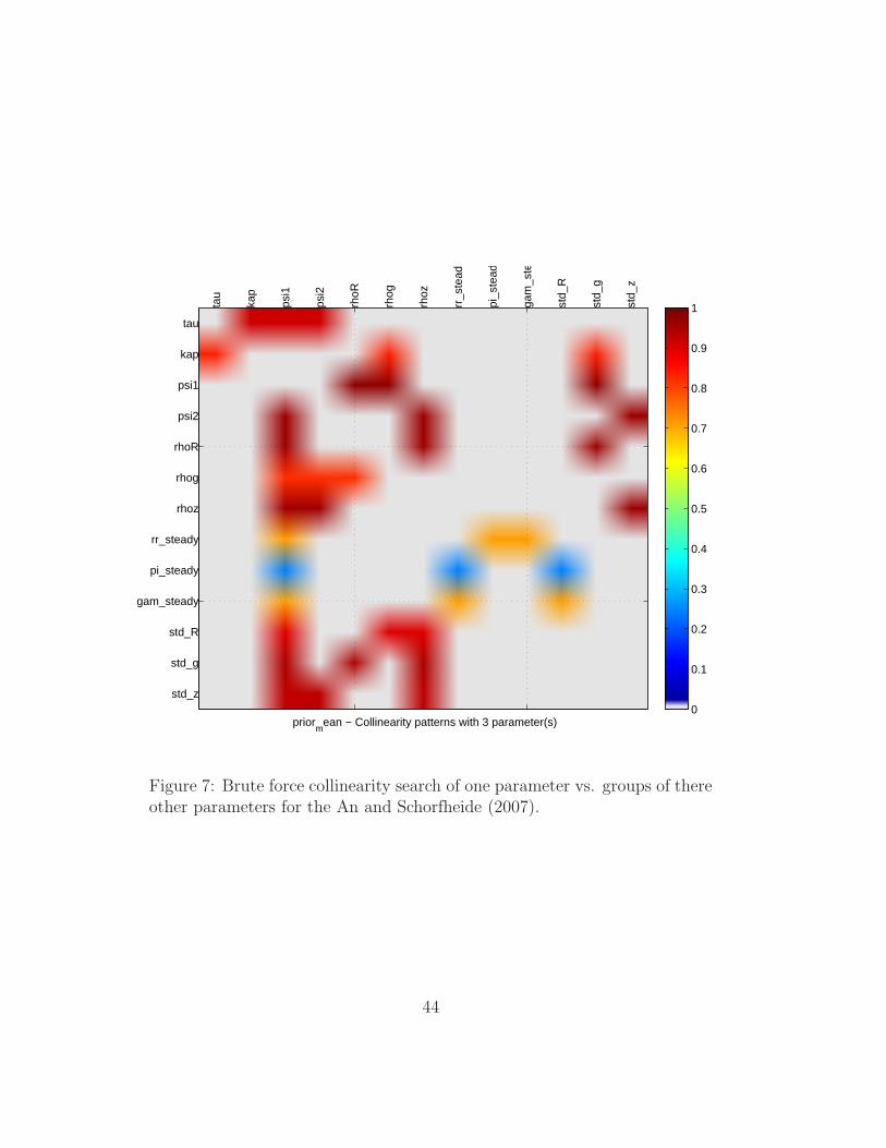
6.2.2 Advanced Monte Carlo procedure
An example of syntax for the advanced Monte Carlo identification procedure
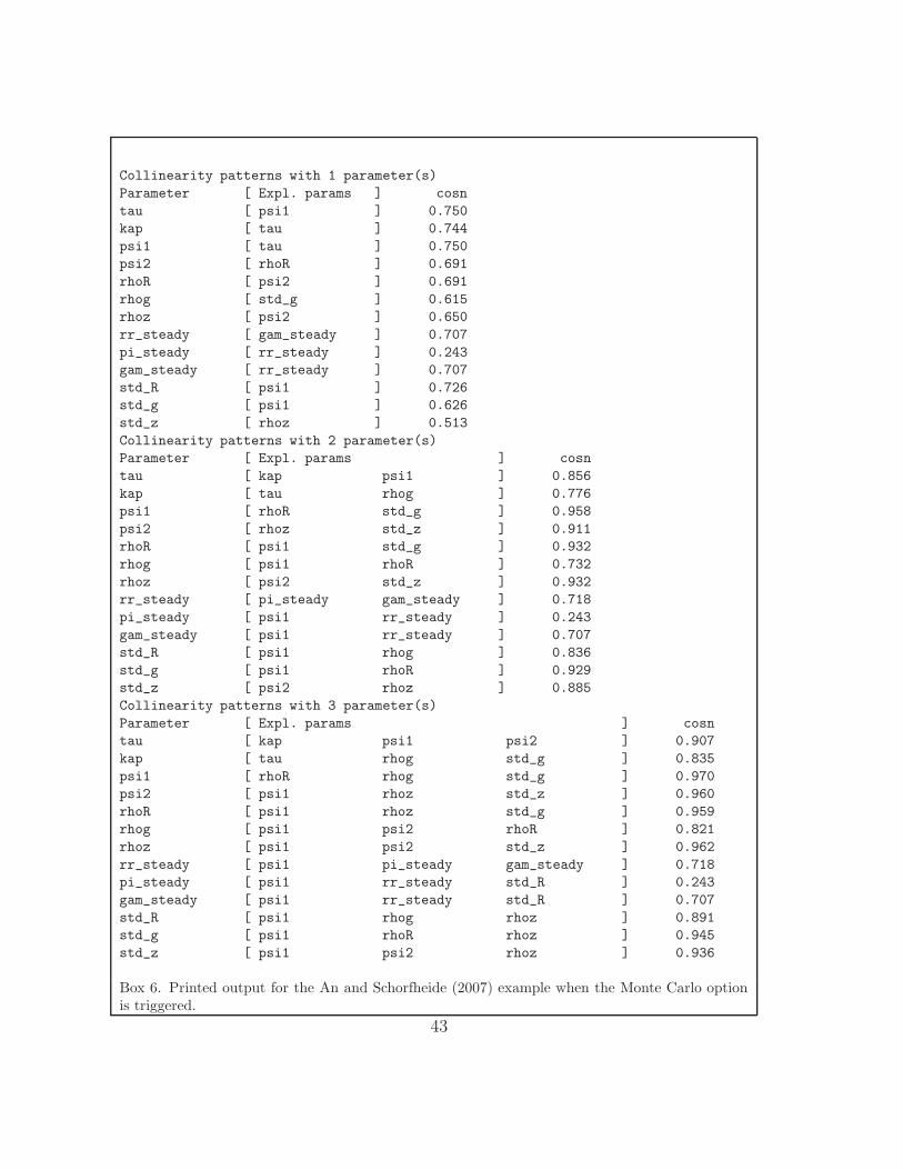
is shown in Syntax 4. For the point-estimate at the prior mean, with the ad-
vanced option, the brute force collinearity analysis a la Iskrev is displayed on
the command window (Box 6) and in graphical form (Figure 7). The latter
is specially informative: in particular we can note the correlation links that
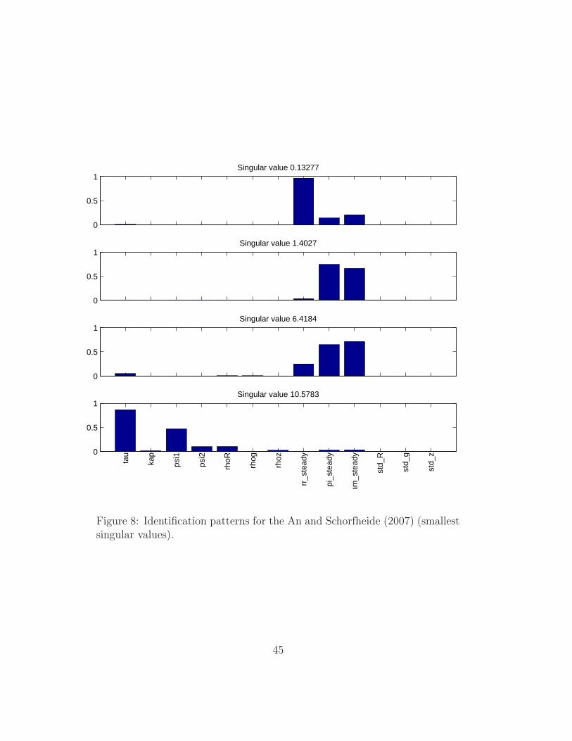
involve ψ1, ψ2 and the autoregressive parameter ρR. The identification pat-
terns a la Andrle are also shown: when the number of estimated parameters
is larger than four, the identification patterns are shown using two panels,
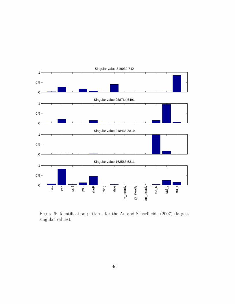
one for the smallest singular values (Figure 8) and the second for the largest
ones (Figure 9). The former spans the weakest identifiable patterns, the
latter spans the strongest ones. Note that these identification patterns take
the SVD of the Hessian. Later on we will see somewhat different patterns
obtained taking the SVD of the Jacobian J(q).
...
identification(advanced=1,max_dim_cova_group=3,prior_mc=250);
...
Syntax 4. Advanced Identification syntax for Monte Carlo identificationanalysis of the An and Schorfheide (2007) example.
42
Collinearity patterns with 1 parameter(s)
Parameter [ Expl. params ] cosn
tau [ psi1 ] 0.750
kap [ tau ] 0.744
psi1 [ tau ] 0.750
psi2 [ rhoR ] 0.691
rhoR [ psi2 ] 0.691
rhog [ std_g ] 0.615
rhoz [ psi2 ] 0.650
rr_steady [ gam_steady ] 0.707
pi_steady [ rr_steady ] 0.243
gam_steady [ rr_steady ] 0.707
std_R [ psi1 ] 0.726
std_g [ psi1 ] 0.626
std_z [ rhoz ] 0.513
Collinearity patterns with 2 parameter(s)
Parameter [ Expl. params ] cosn
tau [ kap psi1 ] 0.856
kap [ tau rhog ] 0.776
psi1 [ rhoR std_g ] 0.958
psi2 [ rhoz std_z ] 0.911
rhoR [ psi1 std_g ] 0.932
rhog [ psi1 rhoR ] 0.732
rhoz [ psi2 std_z ] 0.932
rr_steady [ pi_steady gam_steady ] 0.718
pi_steady [ psi1 rr_steady ] 0.243
gam_steady [ psi1 rr_steady ] 0.707
std_R [ psi1 rhog ] 0.836
std_g [ psi1 rhoR ] 0.929
std_z [ psi2 rhoz ] 0.885
Collinearity patterns with 3 parameter(s)
Parameter [ Expl. params ] cosn
tau [ kap psi1 psi2 ] 0.907
kap [ tau rhog std_g ] 0.835
psi1 [ rhoR rhog std_g ] 0.970
psi2 [ psi1 rhoz std_z ] 0.960
rhoR [ psi1 rhoz std_g ] 0.959
rhog [ psi1 psi2 rhoR ] 0.821
rhoz [ psi1 psi2 std_z ] 0.962
rr_steady [ psi1 pi_steady gam_steady ] 0.718
pi_steady [ psi1 rr_steady std_R ] 0.243
gam_steady [ psi1 rr_steady std_R ] 0.707
std_R [ psi1 rhog rhoz ] 0.891
std_g [ psi1 rhoR rhoz ] 0.945
std_z [ psi1 psi2 rhoz ] 0.936
Box 6. Printed output for the An and Schorfheide (2007) example when the Monte Carlo optionis triggered.
43
tau
tau
kap
kap
psi1
psi1
psi2
psi2
rhoR
rhoR
rhog
rhog
rhoz
rhoz
rr_s
tead
y
rr_steady
pi_s
tead
y
pi_steady
gam
_ste
ady
gam_steady
std_
R
std_R
std_
g
std_g
std_
z
std_z
priorm
ean − Collinearity patterns with 3 parameter(s)
0
0.1
0.2
0.3
0.4
0.5
0.6
0.7
0.8
0.9
1
Figure 7: Brute force collinearity search of one parameter vs. groups of thereother parameters for the An and Schorfheide (2007).
44
0
0.5
1Singular value 0.13277
0
0.5
1Singular value 1.4027
0
0.5
1Singular value 6.4184
0
0.5
1
tau
kap
psi1
psi2
rhoR
rhog
rhoz
rr_s
tead
y
pi_s
tead
y
gam
_ste
ady
std_
R
std_
g
std_
z
Singular value 10.5783
Figure 8: Identification patterns for the An and Schorfheide (2007) (smallestsingular values).
45
0
0.5
1Singular value 319032.742
0
0.5
1Singular value 258764.5491
0
0.5
1Singular value 248433.3819
0
0.5
1
tau
kap
psi1
psi2
rhoR
rhog
rhoz
rr_s
tead
y
pi_s
tead
y
gam
_ste
ady
std_
R
std_
g
std_
z
Singular value 163568.5311
Figure 9: Identification patterns for the An and Schorfheide (2007) (largestsingular values).
46

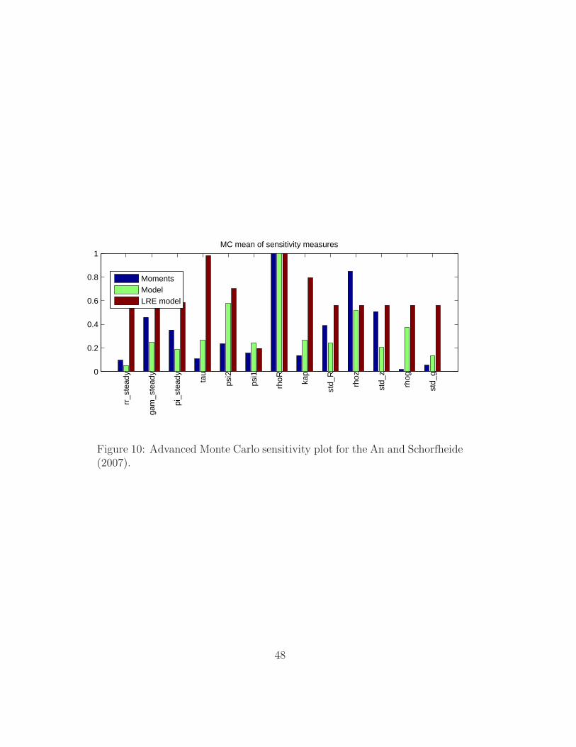
When the advanced Monte Carlo is performed, first the sensitivity plot
is shown: in the advanced mode, sensitivities are shown not only for the
moments (i.e. based on J(q)) but also for the model and LRE model (i.e.
based on J2 and JΓ), see Figure 10.
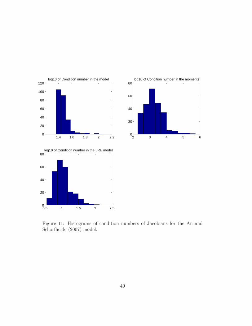
The advanced Monte Carlo diagnostics proceeds by analyzing the condi-
tion number of the Jacobians.
• First the histogram of the condition numbers across the Monte Carlo
sample is shown (Figure 11).
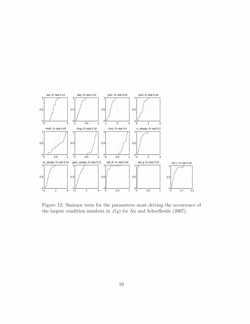
• Second the sensitivity of the condition number versus parameters is
analyzed applying the Monte Carlo filtering technique (Ratto, 2008):
the parameters that mostly drive the occurrence of the largest condition
numbers are searched. An example for the condition number of J(q)
is shown in Figure 12, where one can see that large values for ρR and
ρz are most responsible for the largest condition number, i.e. possibly
driving to weaker identification.
47
0
0.2
0.4
0.6
0.8
1
rr_s
tead
y
gam
_ste
ady
pi_s
tead
y
tau
psi2
psi1
rhoR ka
p
std_
R
rhoz
std_
z
rhog
std_
g
MC mean of sensitivity measures
MomentsModelLRE model
Figure 10: Advanced Monte Carlo sensitivity plot for the An and Schorfheide(2007).
48
1.4 1.6 1.8 2 2.20
20
40
60
80
100
120log10 of Condition number in the model
2 3 4 5 60
20
40
60
80log10 of Condition number in the moments
0.5 1 1.5 2 2.50
20
40
60
80log10 of Condition number in the LRE model
Figure 11: Histograms of condition numbers of Jacobians for the An andSchorfheide (2007) model.
49
0 50
0.5
1tau. D−stat 0.12
0 0.5 10
0.5
1kap. D−stat 0.15
1 2 30
0.5
1psi1. D−stat 0.25
0 1 20
0.5
1psi2. D−stat 0.16
0 0.5 10
0.5
1rhoR. D−stat 0.43
0 0.5 10
0.5
1rhog. D−stat 0.16
0 0.5 10
0.5
1rhoz. D−stat 0.4
0 2 40
0.5
1rr_steady. D−stat 0.2
0 2 40
0.5
1pi_steady. D−stat 0.14
0 2 40
0.5
1gam_steady. D−stat 0.11
0 0.5 10
0.5
1std_R. D−stat 0.24
0 0.5 10
0.5
1std_g. D−stat 0.32
0 0.2 0.40
0.5
1std_z. D−stat 0.38
Figure 12: Smirnov tests for the parameters most driving the occurrence ofthe largest condition numbers in J(q) for An and Schorfheide (2007).
50

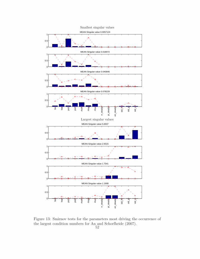
Monte Carlo identification patterns are also displayed, by performing the
Singular Valued Decomposition proposed by Andrle (2010) for J(q) in each
Monte Carlo sample. This provides a sample of eigenvectors associated to the
smallest/largest singular values. The mean and 90% quantile of the distribu-
tion of such eigenvectors is plotted as shown in Figure 13. It is interesting to
note that, in such plot, the patterns seem to maintain some coherence and
consistency across the Monte Carlo sample, suggesting the for this model
the identification pattern is quite uniform over the prior space. Also, it is
interesting to note that, considering J(q), the mean parameters πA,rA and
γQ display clearly their identifiable effect through the first moments, while
using the Hessian (Figure 8), the ‘measure’ of such effect was less notable.
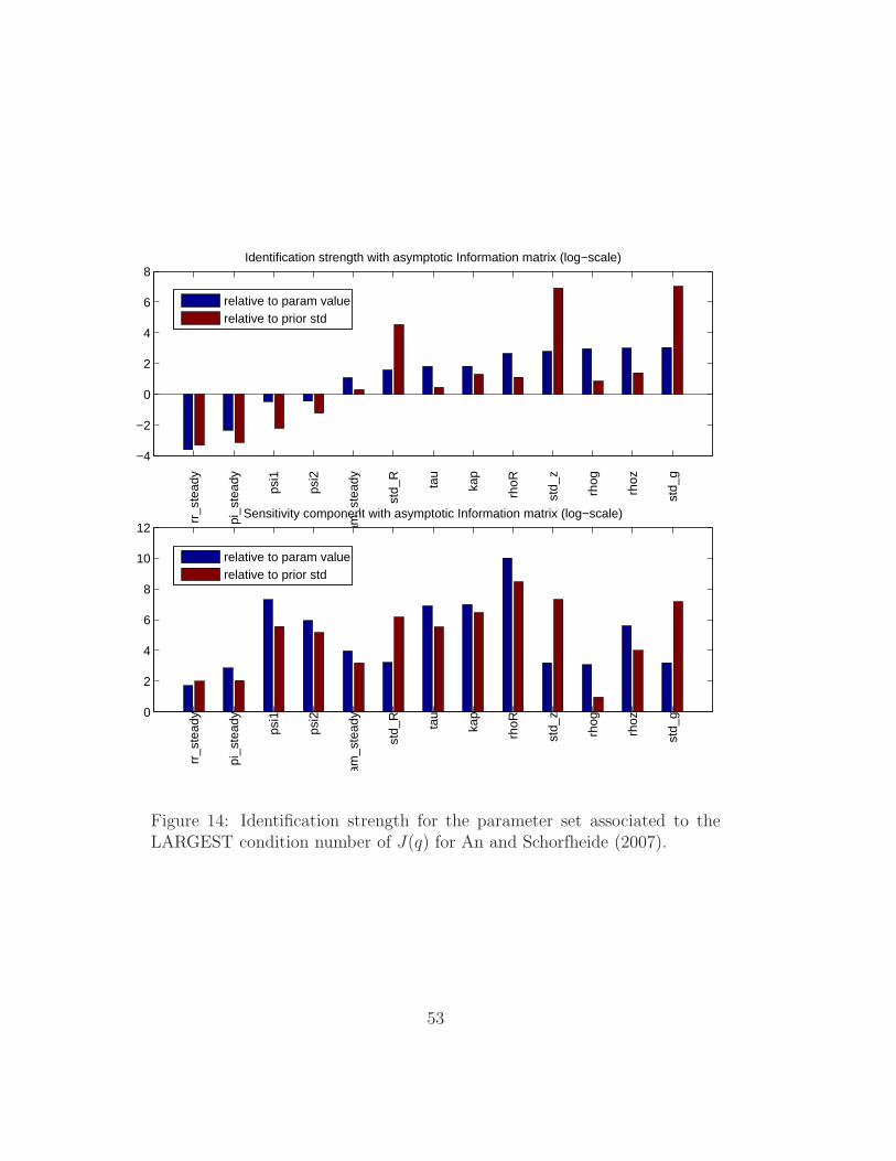
The final set of diagnostics for the advanced Monte Carlo option, point-
estimates are also shown for the parameter combinations associated to the
largest and smallest condition number of J(q). We show in Figures 14-15
the identification strength plots for those two special points, where we can
see that the identification characteristics are fairly similar to each other and
to the prior mean (Figure 5). The main difference distinguishing the ‘worst’
identifiable case in Figure 14 is that the identification strength of φ1 and φ2
drops significantly.
51
Smallest singular values
0
0.5
1MEAN Singular value 0.0057124
0
0.5
1MEAN Singular value 0.018072
0
0.5
1MEAN Singular value 0.040846
0
0.5
1
tau
kap
psi1
psi2
rhoR
rhog
rhoz
rr_s
tead
y
pi_s
tead
y
gam
_ste
ady
std_
R
std_
g
std_
z
MEAN Singular value 0.078229
Largest singular values
0
0.5
1MEAN Singular value 5.6937
0
0.5
1MEAN Singular value 2.9315
0
0.5
1MEAN Singular value 1.7541
0
0.5
1
tau
kap
psi1
psi2
rhoR
rhog
rhoz
rr_s
tead
y
pi_s
tead
y
gam
_ste
ady
std_
R
std_
g
std_
z
MEAN Singular value 1.1908
Figure 13: Smirnov tests for the parameters most driving the occurrence ofthe largest condition numbers for An and Schorfheide (2007).
52
−4
−2
0
2
4
6
8
rr_s
tead
y
pi_s
tead
y
psi1
psi2
gam
_ste
ady
std_
R
tau
kap
rhoR
std_
z
rhog
rhoz
std_
g
Identification strength with asymptotic Information matrix (log−scale)
relative to param valuerelative to prior std
0
2
4
6
8
10
12
rr_s
tead
y
pi_s
tead
y
psi1
psi2
gam
_ste
ady
std_
R
tau
kap
rhoR
std_
z
rhog
rhoz
std_
g
Sensitivity component with asymptotic Information matrix (log−scale)
relative to param valuerelative to prior std
Figure 14: Identification strength for the parameter set associated to theLARGEST condition number of J(q) for An and Schorfheide (2007).
53
−2
0
2
4
6
8
rr_s
tead
y
pi_s
tead
y
gam
_ste
ady
tau
kap
psi2
psi1
std_
R
rhoR
rhoz
std_
g
std_
z
rhog
Identification strength with asymptotic Information matrix (log−scale)
relative to param valuerelative to prior std
−2
0
2
4
6
8
rr_s
tead
y
pi_s
tead
y
gam
_ste
ady
tau
kap
psi2
psi1
std_
R
rhoR
rhoz
std_
g
std_
z
rhog
Sensitivity component with asymptotic Information matrix (log−scale)
relative to param valuerelative to prior std
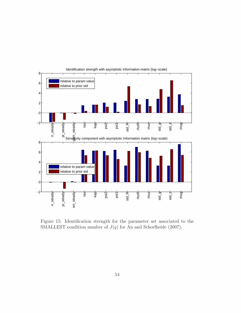
Figure 15: Identification strength for the parameter set associated to theSMALLEST condition number of J(q) for An and Schorfheide (2007).
54
7 Conclusions
We have described in detail the Identification Toolbox developed for analyz-
ing DSGE models under the DYNARe environment. The toolbox provides
a wide set of diagnostic tools to analyze the identification strength of the
model. Advanced options allow to inspect identification patterns, that help
the analyst in tracking the possibly weakest elements of the model parame-
ter set. Moreover, the Monte Carlo option allow to study how identification
features are changed across the entire prior space.
References
An, S. and F. Schorfheide (2007). Bayesian analysis of DSGE models. Econo-
metric Reviews 26 (2-4), 113–172. DOI:10.1080/07474930701220071.
Andrle, M. (2010). A note on identification patterns in DSGE models
(august 11, 2010). ECB Working Paper 1235. Available at SSRN:
http://ssrn.com/abstract=1656963.
Canova, F. and L. Sala (2009, May). Back to square one: identification issues
in DSGE models. Journal of Monetary Economics 56 (4).
Cochrane, J. H. (2007, September). Identification with taylor rules: A crit-
ical review. NBER Working Papers 13410, National Bureau of Economic
Research, Inc.
Florens, J.-P., V. Marimoutou, and A. Peguin-Feissolle (2008). Econometric
Modelling and Inference. Cambridge.
55

Gu, C. (2002). Smoothing Spline ANOVA Models. Springer-Verlag.
Iskrev, N. (2010a). Evaluating the strenght of identification in DSGE models.
an a priori approach. unpublished manuscript.
Iskrev, N. (2010b). Local identification in DSGE models. Journal of Mone-
tary Economics 57, 189–202.
JRC (2010). Development of the combined approach for assessing identifi-
cation in the prior space of model parameters. software prototype. MON-
FISPOL Grant no. 225149 - Deliverable 3.1.1, Joint Research Centre.
Kim, J. (2003, February). Functional equivalence between intertemporal and
multisectoral investment adjustment costs. Journal of Economic Dynamics
and Control 27 (4), 533–549.
Komunjer, I. and S. Ng (2009). Dynamic identification of DSGE models.
unpublished manuscript.
Oakley, J. and A. O’Hagan (2004). Probabilistic sensitivity analysis of com-
plex models: a Bayesian approach. J. Royal Stat. Soc. B 66, 751–769.
Ratto, M. (2008). Analysing DSGE models with global sensitivity analysis.
Computational Economics 31, 115–139.
Ratto, M. and N. Iskrev (2010a). Computational advances in analyzing
identification of DSGE models. 6th DYNARE Conference, June 3-4, 2010,
Gustavelund, Tuusula, Finland. Bank of Finland, DSGE-net and Dynare
Project at CEPREMAP.
56

Ratto, M. and N. Iskrev (2010b). Identification toolbox for DYNARE.
1st MONFISPOL conference, London, 4-5 November 2010. The London
Metropolitan University and the European Research project (FP7-SSH)
MONFISPOL.
Ratto, M. and A. Pagano (2010). Recursive algorithms for efficient identifi-
cation of smoothing spline anova models. Advances in Statistical Analysis.
In Press.
Saltelli, A., P. Annoni, I. Azzini, F. Campolongo, M. Ratto, and S. Taran-
tola (2010). Variance based sensitivity analysis of model output. design
and estimator for the total sensitivity index. Computer Physics Commu-
nications 181 (2), 259 – 270.
Sobol’, I. M. (1990). Sensitivity estimates for nonlinear mathematical mod-
els. Matematicheskoe Modelirovanie 2, 112–118. in Russian, translated in
English in Sobol’ (1993).
Sobol’, I. M. (1993). Sensitivity analysis for non-linear mathematical mod-
els. Mathematical Modelling and Computational Experiment 1, 407–414.
English translation of Russian original paper Sobol’ (1990).
Storlie, C. B. and J. C. Helton (2007). Multiple predictor smoothing methods
for sensitivity analysis: description of techniques. Reliability Engineering
& System Safety 93, 28–54.
57


[Lambda]](https://img.pdfslide.net/doc/110x75/55cf8c955503462b138df368/clase-2rbc-intro-dynaremacroavanlambda.jpg)