Draft for workshop

TABLE OF CONTENTS

MONITORING AFRICAN FOOD AND AGRICULTURAL POLICIES (MAFAP)...................................4

PROJECT METHODOLOGY: CONCEPT PAPER.......................................................................................4

BACKGROUND AND CONTEXT................................................................................................................4

SUMMARY OF METHODOLOGICAL CHALLENGES.............................................................................7

Price incentives and disincentives................................................................................................................8Public expenditures in support of food and agriculture sector development...............................................93. Country reports and development indicators..........................................................................................10

PART 1. PRICE INCENTIVES AND DISINCENTIVES IN THE FOOD AND AGRICULTURAL SYSTEM........................................................................................................................................................12

1.1. Introduction.........................................................................................................................................121.2. Explicit price incentives and disincentives..........................................................................................151.3. Excess costs.........................................................................................................................................161.4. Accounting for different market levels and monopolistic pricing.......................................................181.5. Treatment of non-tradables and non-traded commodities...................................................................19

Discussion Question 1.4: How best can MAFAP capture the various aspect of non-tradability?.........211.6. Exchange rate misalignment................................................................................................................211.7. Inter-sectoral incentives and disincentives..........................................................................................221.8. Input market incentives and effective protection................................................................................23

The Policy Analysis Matrix (PAM) in the VCA context........................................................................241.9. Treatment of primary versus processed products: the Value Chain Analysis (VCA) approach.........25

Protection pass-through..........................................................................................................................271.10. Treatment of externalities and public goods.....................................................................................271.11. Beyond the border costs....................................................................................................................291.12. Trade restrictiveness..........................................................................................................................301.13. Modelling policy interventions.........................................................................................................301.14. Data needs.........................................................................................................................................311.15. Summary of incentive / disincentive indicators to be developed......................................................321.16. Other issues.......................................................................................................................................33

PART 2. GOVERNMENT EXPENDITURES IN SUPPORT OF FOOD AND AGRICULTURE SECTOR DEVELOPMENT..........................................................................................................................................34

2.1. Purpose and scope...............................................................................................................................342.2. Proposed classification and disaggregation.........................................................................................342.3. Definitions of categories.....................................................................................................................382.4. Complete coverage of institutions, administrative levels and financing instruments.........................382.5. Budgetary transfers versus revenue forgone.......................................................................................382.6. Mapping aid onto national expenditures.............................................................................................392.7. Types of external aid...........................................................................................................................422.8. Budget planning versus actual spending.............................................................................................432.9. Treatment of policy administration costs............................................................................................432.10. Treatment of one-off investments versus recurrent expenditures.....................................................43

2.11. Measuring efficacy, efficiency and effectiveness of public expenditures.........................................432.12. Classifying support to the food and agriculture sector......................................................................442.13. Data needs and sources......................................................................................................................442.14. Information gaps................................................................................................................................44

PART 3. COUNTRY REPORTS AND DEVELOPMENT INDICATORS.................................................50

3.1. Overview.............................................................................................................................................503.2. Coverage of proposed performance and development indicators.......................................................503.3. Proposed structure of country reports.................................................................................................53ANNEX 1. Agricultural policies and support for individual commodities................................................55ANNEX 2. MAFAP methodology and calculations..................................................................................55

ANNEX 1. POLICY DISTORTIONS AND THE “DEVELOPMENT GAP” IN GHANA.........................56

ANNEX 2. PRICE DECOMPOSITIONS FOR EXPORTABLE, IMPORTABLE AND NON-TRADABLE........................................................................................................................................................................61

ANNEX 3. BEYOND THE BORDER EFFECTS........................................................................................65

ANNEX 4: PROTECTION PASS THROUGH ALONG VALUE CHAINS...............................................66

TablesTable 2.1. CRS Agriculture-Specific Categories.......................................................................................11Table 2.2. CRS sectors potentially relevant for agriculture.......................................................................11

Figures

Figure 1.1. Nominal rates of assistance to exportable, import-competing and alla agricultural products, African region, 1955 to 2004*....................................................................................................................11Figure 1.2. Nominal rates of assistance to agriculture, by region (%), 1980-84 and 2000-04...................11Figure 1.3. Price decomposition for an imported product..........................................................................11Figure 1.5. Suppression of a potential export as a result of a.....................................................................11Figure 1.6. An example of a suppressed rural surplus...............................................................................11Figure 1.7. Production process of a typical economic agent......................................................................11Figure 1.8. Classic three-row PAM............................................................................................................11Figure 1.9. Schematic value chain..............................................................................................................11Figure 1.10. Summary data structure of a (simplified) multi-period VCA................................................11Figure 1.11. Externalities: A simple classification.....................................................................................11Figure 2.1. Mapping aid on national expenditures.....................................................................................11Figure C.1. Allocation of the f.o.b. export price for cocoa beans, 1955-2004...........................................11Figure C.2. Allocation of FOB export price, based on data on export tax payments in the 1990s............11Figure A.3. Rice prices...............................................................................................................................11Figure A.4. Maize prices............................................................................................................................11

Boxes

How would the adopted indicators inform policy analysis?........................................................................6Box 2.1. Proposed classification of public expenditures in support of the food and agriculture sector....11Box 2.2. Proposed classification of public expenditures in support of the fisheries sector.......................11Box 2.3. Proposed classification of public expenditures in support of the forestry sector........................11Box 2.4. Simplified classification for historical data.................................................................................11Box 3.1. Coverage of proposed performance and development indicators................................................11Box 3.2. Proposed structure of country reports..........................................................................................11

2

3

Acknowledgments

This Concept Paper been developed in the context of the “Monitoring African Food and Agricultural Policies” (MAFAP) project.

It is the result of the work of a team of FAO and OECD staff members including Jean Balié, Piero Conforti and Cristian Morales Opazo, from the Economic and Social Development Department, and Lorenzo Bellú, Materne Maetz and Piera Tortora from the Technical Cooperation Department, and Joanna Komorowska from the Trade and Agriculture Directorate of the OECD.

The preparation of this report was coordinated by Jonathan Brooks from the Trade and Agriculture Directorate of the OECD OECD.

MONITORING AFRICAN FOOD AND AGRICULTURAL POLICIES

(MAFAP)

PROJECT METHODOLOGY: CONCEPT PAPER

BACKGROUND AND CONTEXT

To achieve agricultural development, sustainable use of natural resources and enhanced food security, governments can use two main categories of instruments to influence change in the food and agriculture sector: policies and supporting public expenditure.

To attain specific development objectives, governments use policies to change the rules governing the economy as a whole (macro-economic policy) or governing a particular economic sector (sector policies), in order to guide and modify the behaviour and decisions of the agents operating in the economy. This can be done either by establishing a legal framework to which economic agents have to abide (e.g. food quality or safety norms, property rights) lest they run the risk of legal prosecution or fines, through institutional reform or by providing incentives or disincentives to certain behaviours via price and trade policies, input and output marketing policies, social policies (income transfers, safety nets, social security schemes) and finance policies.

Public expenditure, on the other hand, can be used to avail goods and services to the food and agriculture sector to support the implementation of government policies and facilitate achievement of development objectives. This expenditure may include the provision of public goods through public investment in infrastructures for example or private benefits such as, subsidies or income transfers.

To monitor their actions and ensure that they are consistent and contribute adequately to the development objectives pursued, it is therefore essential for governments to be fully informed on the incentives or disincentives that the packages of policies they implement provide to the economy, and on the consistency, efficacy and adequacy of the way in which they spend their public resources.

Some of the key questions that they need to be able to respond to are:

▪ Do policies in place provide incentives to the production, processing and marketing to key food and agricultural value chains or do they penalize them?

▪ Who in the most strategic value chains benefits from the policies in place? Producers, processors, traders or consumers?

▪ Which policies should be changed for the incentive structure in the food and agriculture sector to be more in line with objectives pursued by the government?

▪ Is public expenditure spent in a way that addresses the key issues faced by the food and agriculture sector? (i.e. what is the most efficient way to improve farmer incomes, input subsidy or investing in a road?)

▪ Is public investment focusing on key investment needs?

4

▪ Are policy incentives and public expenditure coherent or do they in some cases provide contradictory signals to the economy, resulting in wastage of rare public resources?

▪ Are public resources spent efficiently, or is an excessive share of it used for administration?The Monitoring African Food and Agricultural Policies (MAFAP) project is a joint initiative of FAO

and OECD supported by the Bill and Melinda Gates Foundation. The fundamental aim of MAFAP is to help policymakers and other stakeholders ensure that policies and financial investments are fully supportive of agricultural development, the sustainable use of natural resources and enhanced food security. The information generated through the project should assist African governments in not just fulfilling their commitments to increase the share of national resources devoted to agriculture and rural development, but also in allocating their resources wisely. It should also be useful to donors who have pledged to reverse the relative decline in funding to the sector.

MAFAP seeks to establish a system for the regular monitoring of food and agricultural policies in Africa, providing information that can inform policy dialogue at national, regional and pan-African levels, and make a valuable contribution to the Comprehensive Africa Agriculture Development Programme (CAADP) of the New Partnership for Africa Development (NEPAD). The information generated should also be of value to donors and other stakeholders. Central to the monitoring system will be the production of a triennial monitoring report and in-depth national studies for a rising number of countries.

The MAFAP analysis will be underpinned by a suite of food and agricultural policy and development indicators of value to all stakeholders, including national governments and development partners. These indicators will provide quantitative information on agricultural policies, including both market interventions and budgetary expenditures, and will measure the scale of development challenges faced by the agricultural sector. The proposed indicators will provide the underlying basis for addressing two overarching questions about policy choices and investment decisions. First, are current agricultural policies the most appropriate for addressing the country’s policy objectives with respect to development, food security, poverty reduction and natural resource use? If not, what reforms would help? Second, are expenditures being effectively targeted to areas where the need is greatest and potential returns are the highest?

A central principle is that these indicators should be harmonized across countries, in order to permit a comparative assessment of policy priorities and investment needs, and to facilitate exchange on policy experiences. Another important function of the indicators is to establish a quantitative record of policies and investments that have been put in place and to maintain that record over time. Such information is a pre-requisite for a long-term assessment of whether instruments are being targeted to stated objectives and are addressing them effectively, and for the process of learning from policy experiences. The design of the project foresees that the MAFAP Secretariat will work closely with national counterparts in government and relevant research centres in building the necessary indicators.

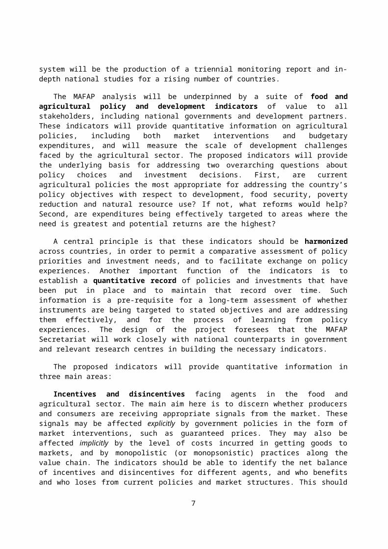
The proposed indicators will provide quantitative information in three main areas:

Incentives and disincentives facing agents in the food and agricultural sector. The main aim here is to discern whether producers and consumers are receiving appropriate signals from the market. These signals may be affected explicitly by government policies in the form of market interventions, such as guaranteed prices. They may also be affected implicitly by the level of costs incurred in getting goods to markets, and by monopolistic (or monopsonistic) practices along the value chain. The indicators should be able to identify the net balance of incentives and disincentives for different agents, and who benefits and who loses from current policies and market structures. This should highlight the need or otherwise for policy reforms, for public investments to reduce costs, and for structural reforms to curb monopoly power.

5

Public expenditures in support of the food and agriculture sector. The indicators of public expenditures will make it possible to keep track of the level and composition of expenditures in support of food and agriculture sector development, and to establish a link between aid allocations and national expenditures. These indicators should make it possible to see whether resources are being allocated to priority areas, whether they address investment needs, and whether they are consistent with the system of incentives that is in place. They should also reveal whether aid allocations are coherent with national priorities.

Development indicators in key areas such as sectoral performance, poverty, inequality, food security; health & human development; and the environment and natural resources. These indicators should show progress in attaining development objectives, as well as the scale of outstanding challenges.

The way in which the proposed indicators would inform policy analysis is illustrated in Box 1.

How would the adopted indicators inform policy analysis?

The different types of MAFAP indicators are complementary:

· Measures of explicit incentives and disincentives, and of market development gaps, indicate potential areas for policy action. In the case of explicit policy interventions, there may be a need for assessing their effectiveness in reaching given objectives and a possible case for reforms, while in the case of market failures or high transactions costs, there may be reasons for reform through institutional or regulatory changes (e.g. a curbing of monopoly powers), or for new investments in public goods to reduce costs and bridge the development gap.

· The measures of disincentives can be associated with a range of market development indicators such as the condition of rural infrastructure, the share of farm operations receiving credit, and measures of the functioning of land markets or water allocation. Changes in these measures would provide information on progress in reducing disincentives.

· The disaggregated measurement of government expenditures would make it possible to contrast the actual allocation of money, including external assistance, with areas of need. Thus there would be a link between the market development gap and efforts to bridge that gap.

How would this work in practice? Taking the output market as an example, domestic prices may be high / low relative to landed border prices due to either formal price policies or high transport and other transaction costs. Policies affecting prices include import tariffs, export taxes and procurement regimes. Transport costs may be excessive due to inadequate roads and other infrastructure deficiencies, while other transaction costs may be excessive for reasons such as sanitary and phytosanitary (SPS) regulations, a lack of competition or limited access to price discovery mechanisms. A reduction in distortions to price incentives may be achieved through the reform of price policies, or by reforms and public investments that reduce excessive transaction costs (market development gaps). Market development indicators can help identify priorities for such action.

By measuring (dis)incentives across multiple domains, it should be possible for policymakers to identify where the distortions in the system are greatest and where the most important priority areas are, be they in the area of commodity policies, macro policies, structural policies or regulatory reforms. It should also facilitate comparative analysis, so that countries can share experiences on the basis of a common analytical framework.

The focus on these three domains of indicators reflects the outcome of a scoping project that was undertaken in 2008. The aim of this scoping project was to investigate the information needs and demands of African governments and development partners and suggest a corresponding project design. Among the conclusions of this project were:

· African governments currently have neither adequate information, nor the necessary tools, to analyse the performance of policies affecting the food and agricultural sectors. They recognize the need to develop such information on a regular basis in order to make rational evidence-based

6

policies, and that the development of appropriate indicators is an important pre-requisite for many forms of policy analysis.

· While there is interest in establishing systems for the measurement of explicit food and agricultural policies, such as taxes, subsidies and various border measures, there is a simultaneous recognition that in African countries market incentives and disincentives are determined not just by policies, but by high transaction costs and the capture of rents along value chains. Accordingly, we have suggested a methodological approach for measuring these costs and rents – which we have referred to as a “market development gap” – in a manner that is consistent (and comparable) with the measurement of formal policies.

· An examination of data availability suggests that the proposed methodology can be implemented successfully. However, it may be necessary to undertake one or two cost of production and marketing surveys in some countries, in order to have the data necessary to make a clear distinction between the effects of formal policies and of “development gaps” on market incentives. Beyond some limited surveys, the final project would not involve the collection of primary data. Nevertheless, the depth of analysis possible for each country will depend on the availability and quality of data. Accordingly, the project should make recommendations for where data availability needs to be improved.

The scoping project outlined some general principles for the project’s methodology. This paper provides a more detailed discussion of the principles that were articulated in the scoping report and considers some of the specific measurement issues that will need to be addressed. The primary purpose of this paper is to solicit feedback on the approach and promote a discussion of how some estimation issues might be addressed at the implementation stage.

An important premise is that it is possible to build on existing approaches, including those adopted by the OECD in its measurement of agricultural policies. At the same time, it is perceived that there is value to taking those approaches further: for example in using price information from Value Chain Analysis (VCA) to discern not just the impacts of formal policies on incentives, but of high costs and monopoly rents; and in classifying public expenditures and aid allocations in a way that helps illuminate spending decisions. A major challenge for the workshop is to identify how far is possible to go both in principle (i.e. having a coherent methodology) and in practice (i.e. within data and resource constraints).

The structure of the paper is as follows. Part 1 provides a conceptual discussion of incentives and disincentives in the food and agricultural sector, suggests a suite of indicators to be computed and discusses estimation issues. Part 2 presents a proposal for classifying government expenditures in support of food and agriculture sector development. Part 3 suggests a supporting set of development and performance indicators, with suggestions on how these indicators can be integrated into the country reports envisaged by the MAFAP project.

SUMMARY OF METHODOLOGICAL CHALLENGES

This project proposes to measure government policies in two domains: the first is price incentives and disincentives in the food and agriculture system, where an effort is proposed to go a bit further than standard approaches, which seek to capture the extent of government interventions in markets. The second

7

is an examination of public expenditures in support of food and agriculture sector development, where choices need to be made in terms of defining an economically relevant and feasible classification system. In addition, it is proposed to harness a range of indicators from secondary sources to provide context and to gauge development performance. All this information will need to be integrated into country reports and into the project’s 2012 monitoring report. As a guide to the more technical discussion in the main text, this section highlights some of the main issues that will need to be addressed in each domain of indicator.

Price incentives and disincentives

Standard approaches (such as those employed by OECD and the World Bank) use price gaps between connected markets to measure the extent to which government policies suppress or elevate prices paid and received by agents in the food and agriculture system.1 These effects can be captured via relatively simple indicators such as nominal rates of protection (NRPs).

In an African context, it may also be important to examine other aspects of price incentives and disincentives. For example, potential exporters may see the prices they receive suppressed by high marketing and transaction costs, or as a result of monopsonistic pricing by exporting agencies. Likewise, consumers may pay high prices for food because of high transport and distribution costs.

An aim of MAFAP is to provide as much key information as possible on price determination for major commodities in the food and agriculture system. The indicators computed should capture both explicit (policy) effects on prices paid and received from the producer to the consumer, as well as implicit effects arising from high costs of monopolistic pricing.

A major question is how much further it is possible to go than has been achieved in earlier studies? Previous attempts to monitor the evolution of price gaps have focused on the explicit policy dimension. In-depth Value Chain Analysis (VCA) and Policy Analysis Matrix (PAM) computations can provide more detail on costs and margins, and potentially on excess costs, and even other sources of market failure. Typically however, they are not replicated on an annual basis. A fundamental question, therefore, is how best to combine the benefits of time series indicators based on price gaps with one or two years of relatively detailed information on price determination along the value chain.

Conceptually there are important challenges in measuring the extent to which costs are “too” high: this involves comparing actual costs with an “efficient” benchmark, which might be established via spatial comparisons of costs (either within the country or across countries), via “expert judgement” or on the basis of technical information on how alternative processes could reduce costs.

Nor is it easy to estimate the extent to which prices are affected by monopoly pricing, which involves establishing the price that would obtain under competitive conditions. It may be possible to obtain a guesstimate by looking at, for example, how the producer’s share of the export price has evolved over time. Alternatively, if there are data that can establish directly how prices are affected by policies (i.e. the rate of export taxation is known, or export tax revenues are recorded), then monopolistic rents can be calculated as a residual. A possibility is that we will have a direct estimate of costs, but that the gap between a domestic and international price will reflect a combination of explicit policies and implicit monopolistic rents. In other words, it may not be possible to have a neat disaggregation of all the components of price incentives and disincentives.

A further aspect of African food and agriculture systems that will need to be addressed is the treatment of products that are no traded internationally. Here it is difficult to calculate the effect of government policies via price gaps, because there is no immediately available international reference price.

1 The formalities of notation will need to be clarified.

8

In fact there are two distinct elements of “non-tradability” that need to be considered. One is where a staple food product is not inherently tradable2. In this case a tradable substitute may provide the nearest reference price. Another possibility is that a product may not be traded because of prohibitive transaction costs. In this case, the international price is still relevant but it may be more difficult to compute the (hypothetical) border price which is relevant for price comparisons.

More generally, there are several other aspects of incentives / disincentives that will need to be addressed, and that can be captured by suitable modifications to basic indicators. These include:

· Exchange rate misalignment, which can have a strong impact on economic incentives.

· Inter-sectoral distortions, reflecting the fact that net incentives depend not just on sectoral price incentives, but also on incentives provided to non-agricultural sectors.

· In put markets. It is possible to calculate the outcomes of input market policies on prices received by farmers, wholesalers and retailers, calculating an effective rate of protection which corresponds to the ratio of value added at domestic prices to value added at border prices.

· Treatment of primary versus processed products. This would need to acknowledge that protection at one market level may not pass through perfectly to another.

There are established techniques for capturing these elements (Anderson et al., 2008, OECD, 2006) and MAFAP proposes to draw on existing approaches (unifying terms and notation where necessary).

Further indicators that could be developed that account for externalities in production and consumption. Similarly, there may also be a desire to look at price determination beyond the border. A specific concern is that border prices may not be relevant in the event of a major transnational “transfer pricing” across national borders.

In summary therefore, there is a general question about how ambitious MAFAP should be in measuring indicators of incentives and disincentives facing the food and agricultural sector, and a number of specific questions related to measurement issues.

Public expenditures in support of food and agriculture sector development

In this domain, we propose to capture all public expenditures that are undertaken in support of food and agriculture sector development. That includes expenditures from national budgets, including both central and regional government, regardless of the ministry that implements the policy. It also includes external aid, provided either through local governments or specific projects conducted by international organisation or NGOs.

We propose to capture all expenditures related to the agriculture, be they agriculture-specific or agriculture-supportive more generally. Additionally, we want to capture all public investments in the rural areas, as these may also have an important role in fostering the food and agriculture sector development, even if they are not specific to the sector. The latter information will also help to clarify whether there is a pro or anti-rural bias in supporting expenditures for such important investments as infrastructure, health and education.

In terms of the classification system, we propose a broad distinction between expenditures that are: agriculture-specific, those that are agriculture supportive more generally (but not specific to agriculture)

2 In practice, are “non-tradable” staples are often traded with African neighbours.

9

and, finally those that are unrelated to the agricultural sector. Within the agriculture-specific category, we propose a distinction between support to producers and other agents in the value chain, and general sector support. The agents in the value chain include farmers (producers), input suppliers, processors, consumers, traders, transporters.

The basic principle behind this classification is the OECD one of classifying policies according their economic characteristics, a rule which provides the basis for further policy analysis. The particular categories, however, should be designed to reflect the types of policies applied in African countries as well as potential data availability. Further, the proposed classification aims to distinguish, to the extent possible, between spending on private goods (subsidies) as opposed to public goods, given their different economic effects.

A range of specific issues need to be addressed and are discussed in the main text. These include:

· The need to ensure complete coverage of institutions, administrative levels and financing instruments.

· The need to account for revenue foregone as well as budgetary transfers. The former could include measures such as tax concessions or the government buying fertiliser on international market and selling it to the farmers at a lower price.

· Mapping aid onto national expenditures. Ideally, we wish to be able to identify sources of finance, which implies establishing a correspondence between public expenditures and incoming aid. The basic question is how complete it is possible or practical to be in reconciling these different sources.

· Budget planning versus actual spending. We would like to be able to measure the efficacy of government spending (how much of government allocations is spent), its efficiency (the degree to which it is targeted to stated objectives) and, ultimately, its effectiveness.

· Treatment of policy administration costs. We propose to measure these costs only when associated with the delivery of specific services (e.g. the salaries of extension advisors, inspection officers and researchers).

· Treatment of one-off investments versus recurrent expenditures Both investments and recurrent expenditures should be recorded on the annual basis using actual spending information, while recognising that one-off investments operate differently to recurrent expenditures in terms of their economic impacts.

3. Country reports and development indicators

In this section we present a proposed structure for the country reports that would constitute part of the MAFAP output, and provide a long list of development indicators that could potentially be presented in those reports and maintained online. This information would be harnessed primarily from secondary sources, and coordinated with the CountrySTAT initiative to the extent possible. As far as possible, indicators already in use in the monitoring systems of participating countries, including the M&E system of the Comprehensive Africa Agriculture Development Programme (CAADP) would be used.

The main issues to be addressed here are:

· What are the core indicators that policymakers and development partners need to see for purposes of monitoring development progress?

10

· What are important “ancillary” indicators that can illuminate the analysis? For example the share of rural roads that is paved, can provide useful information on a key determinant of farmers’ participation in markets.

· What is simply basic information that would naturally be covered in a country study anyway?

· Which measures are redundant and should be omitted?

11

PART 1. PRICE INCENTIVES AND DISINCENTIVES IN THE FOOD AND AGRICULTURAL SYSTEM

1.1. Introduction

The MAFAP project proposes to measure price incentives and disincentives within the food and agriculture sector arising explicitly from government interventions in food and agricultural markets and implicitly as a result of possible market failures in those markets. The explicit part is captured in existing approaches to policy measurement (for example the OECD’s calculations of producer support and the World Bank’s calculation of Distortions to Agricultural Incentives (Anderson et al. 2008)). The implicit aspect is new, and reflects the conjecture that market imperfections are likely to be particularly important in the context of African food and agriculture systems.

In practical terms, we propose to undertake measurement in three domains: (i) explicit policy incentives and disincentives, measured relative to those that would obtain in the absence of any market interventions; (ii) implicit disincentives arising from high costs in commodity chains; and (iii) the implicit incentive to one agent and equal and opposite disincentive to another arising from monopolistic or monopsonistic actions along the commodity chain. We propose to measure each of these components in terms of a price metric, and evaluate their relative importance.

In theoretical terms, we can view each of these elements as a potential distortion to incentives, and measure the resulting welfare losses using standard techniques, such as those pioneered by Harberger. Formally, a distortion arises when the marginal social cost of a transaction is not equal to the marginal social benefit, a condition which defines the social optimum. A market is distorted when the allocation of resources diverges from this (unobserved) optimum.3 The second and third elements can be considered as distortions insofar as lower costs and the elimination of monopolistic pricing practices would raise economic welfare.

If we take the example of a country that trades a particular good on the world market, but is too small to influence the world price itself, then, in the absence of transaction costs, the gap between the domestic price and the corresponding “world” price is a measure of the explicit policy incentive. Import protection would be necessary to maintain a higher domestic price, while export taxes would be needed to suppress the domestic price below the world price. In measuring these incentives / disincentives, we propose to follow procedures consistent with those adopted by the OECD in its measures of producer support, by FAO in its Value Chain Analysis (VCA) and Policy Analysis Matrix (PAM) analysis, and by Anderson et al. in the World Bank’s Distortions to Agricultural Incentives (DAI) project. In each case, estimates make allowance for the transaction costs incurred in bringing the domestically produced product to the point at which it competes with the traded product.

The MAFAP project intends to take the measurement of transactions costs a step further by estimating the extent to which there are “excessive” transaction costs within the value chain, stemming from factors

3 The work of Anderson et al. focuses on measuring explicit policy distortions relative to a benchmark of no market intervention, which corresponds to the social optimum in the absence of externalities or other market failures.

12

such as poor infrastructure, high processing costs because of obsolete technology and high costs due to excessive post-harvest losses. These can be considered an implicit disincentive to the extent that they could be reduced by suitable investments. We also propose, where possible and relevant, to estimate the impact of monopoly power on prices paid and received in the value chain when monopoly power exists. This means calculating the difference between monopolistic prices and those that would prevail with competitive pricing.4 We refer to both of these additional components as a “market development gap”. A major question is to what extent can these components be disentangled?

MAFAP aims to provide regularly updated information on these explicit and implicit incentives and disincentives (distortions). This means building on the DAI project, which was global in scope, with an African component which provided specific evidence on the extent of explicit policy distortions in 20 African economies, covering 90% of Sub-Saharan Africa’s population, farm households, agricultural output and overall GDP. The project provided a long time series of information (typically going back to 1955) that underpinned descriptive analysis (country chapters and regional analysis) and has fed into general equilibrium modelling efforts.

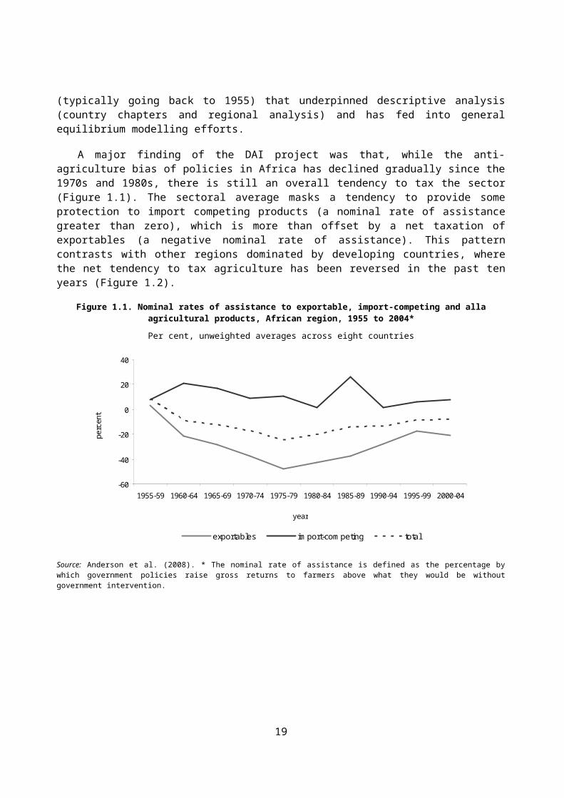
A major finding of the DAI project was that, while the anti-agriculture bias of policies in Africa has declined gradually since the 1970s and 1980s, there is still an overall tendency to tax the sector (Figure 1.1). The sectoral average masks a tendency to provide some protection to import competing products (a nominal rate of assistance greater than zero), which is more than offset by a net taxation of exportables (a negative nominal rate of assistance). This pattern contrasts with other regions dominated by developing countries, where the net tendency to tax agriculture has been reversed in the past ten years (Figure 1.2).

Figure 1.1. Nominal rates of assistance to exportable, import-competing and alla agricultural products, African region, 1955 to 2004*

Per cent, unweighted averages across eight countries

-60

-40

-20

0

20

40

1955-59 1960-64 1965-69 1970-74 1975-79 1980-84 1985-89 1990-94 1995-99 2000-04

year

perc

ent

exportables import-competing total

Source: Anderson et al. (2008). * The nominal rate of assistance is defined as the percentage by which government policies raise gross returns to farmers above what they would be without government intervention.

4 Ideally, it would also be possible to calculate the distortions resulting from uncorrected externalities in production and consumption, but this would be extremely difficult to do across countries is not proposed as part of the project’s core methodology.

13

Figure 1.2. Nominal rates of assistance to agriculture, by region (%), 1980-84 and 2000-04

-40-20

020406080

100120140 1980-84

2000-04

The DAI calculations reveal that transport and other transaction costs (which need to be netted out as part of the calculations) are often particularly high in African countries, and could be reduced significantly through suitable investments, e.g. in physical infrastructure, and through institutional reforms.

There is also evidence from a number of the country case studies of monopoly power being exercised by remaining marketing boards and by private agents within the food and agriculture system, with producers often receiving a low share of the f.o.b. price, even allowing for internal transaction and marketing costs. In some cases, these rents have been interpreted as de facto government policy and therefore registered as a policy distortion.5

MAFAP seeks, as far as possible, to decompose these components in a regular and systematic way. The basic principle is that we want to have a full quantitative representation of the incentives and disincentives in all the major commodity chains in the food and agriculture sector. This will involve combining the OECD approach to measuring commodity level support and protection over time with the FAO’s approach to value chain analysis, thereby obtaining the benefits of horizontal (cross-commodity), vertical (along the value chain) and inter-temporal measurement. We also want to go beyond the effects of explicit government policies and capture implicit disincentives, arising from excessive costs or the capture of economic rents.

By way of illustration, Annex 1 shows the importance of implicit incentives and disincentives in the case of Ghana. The remainder of this section discusses the specifics of constructing an appropriate set of measures. The principles are relatively straightforward, but in practice there are many complications. Some of those complications are discussed in the following sections, although several issues will need to be confronted and addressed at the implementation stage.

5 For example, in the Distortions to Agricultural Incentives project, estimates are made of the rent claimed by Kenya’s National Cereal and Produce Board in the maize market, and of the rent claimed by Uganda’s cooperative unions in the cotton market.

14

Discussion question 1.1: The MAFAP methodology seeks to identify three components of price incentives and disincentives: those deriving from explicit policies, those attributable to excess costs, and those resulting from monopolistic pricing. Is this three-way distinction a helpful way of characterising incentives and disincentives?

1.2. Explicit price incentives and disincentives

The standard basis for measuring price incentives and disincentives (distortions) is the law of one price, which holds that in efficient markets the prices for identical goods should be equal. In the absence of externalities, the law of one price would lead to no distortions and an optimal allocation of resources. In reality, there will always be costs associated with arbitrage between two markets, so another way of stating the law is as follows:

Pa = Pb + T

where T is the cost of transferring from market b to market a.6 The principle can be applied spatially between markets and also to “vertical” transactions along the supply chain.

Take the case of an imported good, with only one market level. Then we can write this as

Pd = Pb + T

where Pd is the domestic price, Pb is the c.i.f. border price expressed in domestic currency and T is the cost of getting the product from the border to the domestic market. Now suppose the government intervenes with a price support policy sustained by a tariff or other border restriction, equal to MPD (market price differential), then the identity becomes

Pd = Pb + T + MPD

Operationally we can calculate MPD as the difference between prices, adjusted for transport and other transaction costs. This is the standard approach adopted by OECD.

= Pd - Pb - T

If the only policy in place is an ad valorem tariff, applied to the border price at a rate of t, the MPD is an estimate of the applied tariff (1 + t) Pb. If it is clear that such a tariff is the only impediment to trade, then an alternative is to compute MPD in this way.

Given prices and transaction costs, one can also calculate two standard indicators, the nominal rate of protection (NRP), which measures the difference between the distorted domestic price and the (in this case is undistorted) world market price adjusted by the cost of bringing the product to the point of competition, as a fraction of the undistorted price, and the nominal rate of assistance (NRA), which is the unit value of production at the distorted price less its value at the undistorted price, expressed as a fraction of the undistorted price.

6 A more accurate way of expressing the law, assuming that the cost of transferring from market a to market b is the same as the cost of transferring from b to a, is | Pa – Pb | ≤ T where T is the cost of transacting between the two markets. In the event that the price gap is less than T then there will be no incentive for arbitrage between the two markets and hence no trade should occur.

15

NRP = (Pd – Pb – T)/ (Pb +T) and NRA = (Pd – Pb – T + S)/ (Pb +T)7

The difference between the two is the inclusion of direct subsidies or taxes (per unit of output), S, in the numerator of the latter estimate. Analogous calculations can be made in the case of an exported commodity. In this case, there would be a taxpayer cost (as opposed to a tariff gain) from maintaining prices above world market levels.

Having calculated NRPs and NRAs for individual commodities, it is possible to attribute a monetary value to the implied transfer by multiplying by an appropriate quantity– production for the farmer, traded volume for the wholesaler and consumption for the final consumer. These amounts can then be aggregated across commodities to obtain an estimate of the transfers to different constituencies – a principle behind the OECD’s calculation of market price support.

An important point to note at this stage is that the incentive/disincentive MPD is calculated as a residual from other variables. Because markets do not adjust to the law of one price perfectly and immediately, such that any arbitrage opportunities are exhausted, the estimate of MPD will inevitably include an element of “noise”. This means that annual point estimates can be misleading, and it is often more instructive to look at average over a period of years. This point is taken up later.

1.3. Excess costs

It is conceptually straightforward to decompose costs (T) into an efficient component, T0, and an “excess”, T1. In the case of an import, we see how domestic prices are naturally raised by transaction (principally transport) costs (T0), but can be further raised by import tariffs (reflected in MPD) and excessive costs, or a “market development gap” (T1) (Figure 1.3). A conservative monetary estimate of the market development gap is T1 × (Q3

d Q3s) – conservative because the imported volume, i.e. the difference

between supply and demand, is reduced by both policies and excessive costs per unit. The export case is the mirror image, with domestic prices lowered, and exported volumes reduced, by both price suppression and export taxes and excessive costs (Figure 1.4, where ET is an Export Tax). Price policy interventions (supported by the necessary trade measures) can of course be applied in either direction.

7 Please note that the procedure followed here is to bring the border price to the domestic market level (Tsakok, 1990). However, it is still under discussion if we would rather consider the border as the point of competition (which would mean adjusting the domestic price).

16

Figure 1.3. Price decomposition for an imported product

Q1s Q2

s Q3s Q1

d Q3d Q2

d Quantity

Price

S

D Pw

Pw+T0 Pw (1+t) +T0 Pw (1+t)+T0 + T1 Excess cost

Figure 1.4. Price decomposition for an exported product

Excess cost

Q1d Q2

d Q3d Q1

s Q3s Q2

s Quantity

Price

S

D

Pw Pw-T0

Pw-T0-ET Pw-T0-ET-T1

17

In practical terms, we need to find a way of decomposing recorded costs into an efficient benchmark level and an excess. One possible indicator is spatial variations in costs within the country being studied, or relative to costs in a neighbouring country. Another way of getting at the possible excess is through value chain analysis (described later).

Discussion Question 1.2. What are the most practical ways of measuring an efficient benchmark for costs that can be replicated across countries in a relatively harmonised way?

1.4. Accounting for different market levels and monopolistic pricing

In general, we are concerned with more than one market level, typically wishing to represent price determination at the retail, wholesale and the producer farmgate levels.

If we assume that the product is imported only at the wholesale level, and that the importing country does not import enough to influence the world price, then, given the world price, we would have simultaneous price determination across three markets. If import protection gives rise to a price gap at the wholesale level (and there are no other policies), then we would thus expect prices to be affected at all levels:

Pdr = Pd

w + Twr

Pdw = Pb + T + MPD

Pdf = Pd

w – Twf

where Pdr, Pd

w and Pdf are domestic retail, wholesale and farmgate prices, and Twr and Twf are the

transactions costs associated with transferring the product from the wholesale to the retail level and from the farmgate to the wholesale market. Note that, under this structure, the price implications of a given absolute amount of price support, MPD, are the same irrespective of the market level at which that support is delivered (the same would not be true if the margins Twr and Twr were multiplicative rather than additive).

The NRP/NRA should be computed at the market level where the government policy is enacted (here the wholesale level). However, we can also compute implied NRPs and NRAs at other market levels. Note that the formulation of identities above contains implicit assumptions about the nature of price transmission from one market stage to another.8 A common practice is to estimate price transmission econometrically both spatially, from international to domestic markets and from one internal market to another, and vertically along the supply chain. Such information can provide complementary insight into how incentives may be affected at market locations and levels other than that where the incidence of policy is recorded.

As with the representation of one market level, we can decompose transaction costs into an efficient component and an excess, and also allow for the passing of monopolistic rent from one level of the market to another. In the three market level example below, R fr corresponds to rent claimed by the retailer at the expense of the consumer, while Rwf corresponds to rent claimed by the wholesaler at the expense of the farmer. In securing these rents, private agents (e.g. such as marketing boards) can induce a price wedge in much the same way as government can.

8 Note that with additive margins the same absolute value of MPD at each level implies a lower proportional NRA at the retail level than at the wholesale level, and a higher NRA at the farmgate level than at the wholesale level.

18

Pdr = Pd

w + T0wr + T1

wr + Rfr

Pdw = Pb + T0 + T1 + MPD

Pdf = Pd

w – T0wf – T1

wf – Rwf

From this representation, we can calculate an implicit burden via higher prices paid by consumers (T1

+ T1wr + Rfr) and lower prices received by farmers (T1

wf – Rwf). [In this case, it is not possible for the retailer to extract rent from the wholesaler because the wholesale price is competitively determined in the international market.]. As with spatial arbitrage, markets do not adjust perfectly and instantaneously along the supply chain, so estimates of R will include noise as well as information on monopolistic behaviour, and data over several years will be more informative than single annual estimates.

A task of MAFAP is to estimate the price incentives and disincentives arising from monopolistic practice in a practical way, without knowledge of underlying supply and demand functions and their associated elasticities. One way of doing this is by observing data on variations in margins over time and establishing a “low” margin that provides a reasonable approximation of costs plus “normal” profit. Another way is to compare margins in the same value chain in other countries, or across similar chains in the same country. Any excess between this and the observed value would be identified as rent.

An approximation of the disincentive that agents at different market levels experience because of excessive costs and rents is provided by the difference between the distorted domestic price (at the level of interest) and the undistorted price plus the policy distortion, as a fraction of the undistorted price plus the policy distortion. This can expressed in the general form:

At wholesale level, for example, this will assume the form:

while at farmgate level:

Examples of how these indicators would be computed are provided in Annex 2.

Discussion Question 1.3. How can we best identify and estimate the extent of monopolistic pricing behaviour? Are there practical ways of dealing with transfer pricing and other cases where we have incomplete information on pricing relationships?

1.5. Treatment of non-tradables and non-traded commodities

So far, the discussion has applied to tradable products. But what about products that are not traded, and where the law of one price cannot be applied in the manner outlined above?

In this case, it is helpful to make a distinction between two distinct aspects of “non-tradability”. One aspect is where the domestic economy produces a good that is not internationally traded but is substitutable with a traded commodity, as is the case for many staples in Sub-Saharan Africa. In this case, it is possible to calculate pass-through from a tradable good to a non-tradable good via cross-elasticities. However, this moves into the realm of estimating policy effects rather than policy incidence. In this case, value chain and

19

cost of production analysis should be able to confirm the existence or otherwise of excess costs and rents, but there is no external reference price from which to compute explicit price interventions. Estimating the incidence of such interventions would require information on government stock accumulation (or sales) and the elasticities of supply and demand.

Another case is where a good is inherently tradable internationally, but policies or excess costs affect incentives in such a way as cut off international trade completely. Figure 1.5 shows the case of a potential export that is suppressed by excess costs incurred in getting the product to market. Inevitable transaction costs reduce the landed price to Pw Ce, associated with net exports of Q0

s Q0d , but further costs

(represented as EC) are sufficiently high to depress the price below the autarky price, such that trade does not occur and the economy remains in autarky. In this case, there is no recorded border price and it is necessary to estimate what would be the relevant reference price (outgoing f.o.b. or incoming c.i.f. price) in the event that trade were to occur. This is feasible, although quantities that would be produced, consumed and traded needs estimates of the underlying supply and demand curves, and these may be difficult to obtain.

Figure 1.5. Suppression of a potential export as a result of a “market development gap”

Excess cost

QoS Qo

D Quantity

S D Price

Pw

Pw- Ce

Pw- EC

A further aspect of non-tradability is where a good is both “tradable” and actually traded, but only a fraction of the product reaches the market, the majority being consumed directly by producing households. Figure 1.6 shows the case where a country is a net importer, yet the transaction costs involved in getting the product to an urban market are sufficiently high to prevent domestic trade from occurring. Here the “urban” market (left panel) faces a domestic price equal to the world price times the relevant tariff plus transaction costs. This market could potentially be supplied by the rural market (right panel), but the rural market remains in autarky because of high transaction costs (ECr).

In this case, market prices are still relevant in capturing the degree of government intervention, but a question then concerns the relevant quantity to be applied when considering the scale of implicit transfers or welfare impacts. In principle, this should be not just those who are in the market but also those who would potentially be in the market at a different set of prices (and costs). It is potentially possible to calibrate a latent net supply function using micro data, with farm household models revealing households’ opportunity costs of participating in markets. Reductions in transactions costs could increase market participation by hitherto autarkic households.

20

Figure 1.6. An example of a suppressed rural surplus

Pd=(1+t)Pw + CU

DU

SU

DR

SR

CR + ECR

Quantity Quantity

Price Price

Discussion Question 1.4: How best can MAFAP capture the various aspect of non-tradability?

Annex 2 reports three simplified spreadsheet examples of a calculation of the price wedges described so far. The first and second examples refer to imported and exported products respectively, which are relatively straightforward. The assumption is that a domestic close substitute is readily available, and differences between the internationally traded and the domestically produced goods may be accounted for by adjustment coefficients. The third example is of a product which is not traded internationally; while its treatment appears similar to the one for imported and exported products, the main difference is in the benchmark price, where credible information needs to be inserted. In the case at hand a close imported substitute is available; hence the benchmark price is the market price of the substitute. Where there is no close substitute, an implicit price will need to be built starting from shadow factor prices.

1.6. Exchange rate misalignment

Exchange rate misalignment can have a strong impact on economic incentives and recorded levels of market price support. Note that an overvalued exchange rate will suppress economic incentives for producers vis-à-vis their international competitors but will lead to a higher estimated value of the NRP.

Hence it can be instructive to calculate protection and assistance at both the actual and long run equilibrium exchange rate and record the difference between the two measures. The equilibrium exchange rate can be calculated in a variety of ways, for example by computing PPP rates or by estimating the equilibrium rate based on economic fundamentals (as done by Orden et al., 2007). Such estimates can, however, be sensitive to specific assumptions. An easier and more practical approach is to provide a complementary indicator which decomposes each domestic price change into three components: that attributable to movements in the world (reference) price, Pw , that due to movements in the exchange rate, E, and finally a residual, R, reflecting policy wedges and imperfect adjustment to the law of one price:

Pd = Pw.E.R

which in proportional (log) terms can be decomposed as

lnPd = lnPw + lnE + lnR

Should a multi-tier foreign exchange rate regime be in place, then an explicit policy-induced price wedge exists, and both the relevant actual exchange rates (for importers and exporters) and the equilibrium

21

exchange rate (understood here as the rate that would obtain in a free market) need to be calculated. Here we propose to follow the approach adopted by Anderson et al. A simple two-tier exchange rate system creates a gap between the price received by exporters and the price paid by importers for foreign currency, changing both the exchange rate received by exporters and that paid by importers from the equilibrium rate that would prevail without this distortion in the domestic market for foreign currency (Bhagwati 1978). The relevant exchange rates for importers and exporters are respectively the discounted parallel market rate and the weighted average of the official exchange rate and the discounted parallel rate according to the proportion of the exporter’s currency that is sold on the parallel market (the parallel market could be the black market if no legal secondary market exists). If a multiple exchange rate system is in place and that system provides for a specific rate for a product that differs from the general rates automatically calculated, then the automatically computed relevant exchange rate is replaced by that industry-specific rate. In the presence of a parallel market rate data are required on the formal retention rate where a formal dual exchange regime is in place, or otherwise a guesstimate of the proportion traded on the black market (premia for which are provided by Easterly 2006 and International Currency Analysis 1993). Given data on the actual exchange rates for exporters and importers, and estimates of supply and demand elasticities for foreign currency, an equilibrium exchange rate can be estimated. In the absence of information on elasticities a reasonable guesstimate is to take the average of the official and secondary market rates.

A viable practical strategy in this area should start from an assessment of conditions in the countries at hand, to verify the extent to which exchange rates are misaligned. In some countries included in MAFAP it is known that the exchange rate is pegged to the Euro through the CFA franc; and efforts are oriented at controlling nominal exchange rates. In such cases the identification of a workable benchmark rate would be particularly useful, as it would allow quantifying the incentive or disincentive effects in agriculture of pegging the currency to the Euro.

1.7. Inter-sectoral incentives and disincentives

The total effect of distortions on the agricultural sector will depend not just on the size of the direct agricultural policy distortions, but also on the magnitude of distortions generated by direct policy measures altering incentives in non-agricultural sectors. Anderson et al. invoke the Lerner Symmetry Theorem, which shows that in a two-sector model an import tariff has the same effect on the export sector as an export tax. Following Anderson et al. we therefore propose to calculate a nominal rate of assistance facing the non-agricultural sector, NRAnon-ag, and a corresponding relative rate of assistance to agriculture, RRAag: 9

RRAag = [(1 + NRAag)/(1+ NRAnon-ag) – 1]

Estimation of NRAnon-ag involves establishing a weighted average across exportable and importable sub-sectors, with weights corresponding to the value of production evaluated at undistorted (reference) prices. In estimating NRAnon-ag we propose to follow treat the service sector as non-tradable, to use tariff data to estimate the NRA for manufactured importables and export tax information to compute an NRA for manufactured exportables. This contrasts with the more data demanding approach adopted for the food and agricultural sector, where NRAs are computed on the basis of price gaps. Nevertheless the RRA should give an idea of the extent to which direct assistance to the sector is offset or reinforced by non-agricultural border policies, and of whether there is a pro- or anti-sectoral bias in the overall orientation of policies. For a check, it is also instructive to compute the ratio of average agricultural tariffs to average non-agricultural tariffs. The collection of tariff data for both downstream versus primary sectors may also reveal tariff

9 In this section NRAag refers to the weighted average nominal rate of assistance across food and agricultural sectors (weighted according to the value of production measured at border prices), while NRAnon-ag refers to the average NRA for all other sectors.

22

escalation and/or de-escalation along value chains and whether there are incentives/disincentives for value addition.10

1.8. Input market incentives and effective protection

In order to understand the overall set of incentives and disincentive facing particular agents, it is helpful to measure, to the extent possible, the margins received by agents as a result of a production process rather than through single commodity prices, and to analyse the whole production process in monetary terms.

Through a production process the agent typically combines inputs and production factors in order to obtain one (or more) outputs. The way he/she combines inputs to get outputs is defined by the production technology.

Figure 1.7. Production process of a typical economic agent

PRODUCTION PROCESS OUTPUT

INPUTS

PRODUCTI ON FACTORS

Knowing the technology and the scale of the operations it is possible to assess in monetary terms the margins of the economic agent for a specific activity. When calculating margins, the prices of different inputs, factors and outputs are weighted by means of physical quantities of the respective goods and services and aggregated in a monetary indicator. By comparing the margins obtained using “observed” market prices with the margins obtained using “reference” prices we obtain a measure of the incentives-disincentives that the agent receives in carrying out a specific activity. This enables us to calculate effective protection indicators such as the Effective Rate of Protection (ERP), which corresponds to the ratio of value added at domestic prices to value added at border prices, where value added is the value of output minus the cost of traded intermediate inputs). As with the NRA, an effective rate of assistance can be computed by allowing for per unit taxes and subsidies in the computation of value added at domestic prices.11

10 It is also possible to compute an agricultural trade-bias index, TBI = [(1 + NRAagx)/(1+ NRAagm) – 1], where NRAagx and NRAagm are the NRAs for the import-competing and exportable parts of the agricultural sector.

11 Few of the African country DAI studies computed ERPs or ERAs. However, this should be possible with suitable value chain analyses for the principal commodity chains. A specific issue is that markets for certain inputs may not exist at all. In the absence of an appropriate domestic price, it will be important to include quantitative analysis of reasons for the lack of functioning of markets

23

The Policy Analysis Matrix (PAM) in the VCA context

Margins, calculated as difference between revenues, intermediate inputs and factor costs can be analyzed by means of the “Policy Analysis Matrix” (PAM) (Figure 1.8). The PAM will be used, in the VCA context, to summarize results, analyse margins and work out nominal and effective rates of protection (NRP, ERP), as well as selected competitive and comparative advantage indicators 12. Calculations carried out and reported in a PAM relate to specific commodities, agents or any other relevant aggregate of agents, such as layers or segments of specific value chains or whole value chains 13. The PAM in Figure 1.8 is presented in its classic three-row format: 1) Revenues and costs at “market” prices; 2) revenues and costs at “reference” prices and 3) Differences between 2) and 1). The PAM can be adapted and extended to host revenues and costs calculated with different price configurations and to report different balances relevant for monitoring incentives-disincentives, highlighting the various components (explicit policy, excess costs, etc.) of the wedge between observed and reference prices. Indicators of nominal, effective protection and competitiveness are calculated combining info reported in the various cells (A, B, C, etc) of the PAM. Need to spell out those indicators.

Figure 1.8. Classic three-row PAM

REVENUES

COSTS PROFITS

Tradable Inputs DomesticFactors &Not tradable inputs

1) Revenues and costs at “Observed” market Prices

A B C D

2) Revenues and costs at “Reference”

E F G H

3) Gap I J K L

A specific issue is that markets for certain inputs may not exist at all. In the absence of an appropriate domestic price, it will be important to include quantitative analysis of reasons for the lack of functioning of markets.

1.9. Treatment of primary versus processed products: the Value Chain Analysis (VCA) approach

For many products a degree of processing exists between the farmgate and the final consumption product. This is especially true for livestock and dairy products, but applies also to sugarcane, cotton etc. 14.

12 The FAO “VCA” software is a suitable tool to store multi-period VCA data, carry out VCA analyses and work out PAMs and related protection and competitiveness indicators. It builds upon the long-lasting experience of FAO in carrying out Value chain Analyses for agricultural and rural development all around the world. The VCA software, as well as other relevant material on value chain analysis, is available through EASYPol, the web-based repository of resource materials for policy making, at www.fao.org/easypol.

13 For a detailed explanation of the PAM approach see Monke and Person (1989).

24

In making incentive-disincentive comparisons it is essential to compare the product at the same degree of processing, so an adjustment for weight and processing costs needs to be made.

The OECD has a specific approach for dairy products, where there is little international trade in fluid milk. In this case, a reference price for fluid milk is established on the basis of a weighted combination of the prices of butter, cheese and skimmed milk powder.

The Value Chain Analysis (VCA) provides a framework to consistently analyse vertically integrated activities. The commodity passing from an agent to another constitutes a “vertical” link between two agents (figure 2). This “vertical” link implies that incentives-disincentives affecting agents in the processing phase are affecting also primary commodity producers and vice-versa. This implies that, in order to measure the protection enjoyed by primary producers, the margins of processors also need to be known (and vice-versa). This implies measuring the inputs and outputs of processing activities.

The Value Chain Analysis (VCA) accounting framework has been widely utilized as an approach to consistently analyze the activities of “vertically” linked agents15. MAFAP can adopt this to analyse production-processing activities, to work out margins at the different stages of a commodity chain, as well as to calculate aggregate margins for the whole value chain. These calculations can be carried out using “observed” market prices, as well as “reference” prices.

Figure 1.9. Schematic value chain

Country

Border

Producers

Consumers

Exporters/Importers

Processors

Primary product collectors

Retailers

Wholesalers

Global Market

VCA approach in a multi-period framework. As MAFAP aims at monitoring policies over time, the methodological approach must ensure that the calculation of relevant VCA incentive-disincentive

14 The OECD has a specific approach for dairy products, where there is little international trade in fluid milk. In this case, a reference price for fluid milk is established on the basis of a weighted combination of the prices of butter, cheese and skimmed milk powder

15 See e.g. the report DGPSA (2007): Analyse des impacts des politiques de développement agricole et rural et des filières Agro-sylvo-pastorales sur la pauvreté et la sécurité alimentaire: résultats synthétiques . Ouagadougou, Burkina Faso 2007, and related Value Chain Analysis reports.

25

indicators be possible in a multi-period framework. Considering that building a value chain framework is quite a data and resource-intensive process, MAFAP will adopt a strategy to update more frequently those value chain data likely to significantly change from one year to the other. Data, more structural in nature, will be updated less frequently. Figure 3 summarizes the data structure of a multi-period value chain framework.

In general terms the type of data required to build a VCA framework are:

1) Prices (both “observed” and “reference”) of the inputs entering the various activities along the chain (p1, p2 ....);

2) Prices (both “observed” and “reference”) of outputs of the various activities (pr , ps .......) 3) Quantities of inputs (q1, q2, ...) per unit of activity (e.g. per hectare, per ton of processed output, etc),4) Quantities of outputs per unit of activity (qr , qs .......) 5) Scale factors at different levels, to reflect in the VCA accounting framework the actual (real life) scale

of each activity at various levels. Scale factors, which are specific to each value chain and the way the VC has been modelled, are for instance: Number of hectares of cotton per “small farmer”, number of small farmers in the country, tons processed by the typical ginnery in a given zone, etc.

Figure 1.10. Summary data structure of a (simplified) multi-period VCA

.......

Price quantity value Price quantity value Price quantity value

Inputs Inputs Inputsp1 x q1 = v1 p1 x q1 = v1 p1 x q1 = v1 .......p2 x q2 = v2 p2 x q2 = v2 p2 x q2 = v2

... ... ... ... ... ... ... ... ... x Q x Q x Q

Output Output Output .......py x qy = Vy py x qy = Vy py x qy = Vy

pz x qz = Vz pz x qz = Vz pz x qz = Vz

Margins Margins Margins(Vy + Vz) - (v1 + v2 + ....) (Vy + Vz) - (v1 + v2 + ....) (Vy + Vz) - (v1 + v2 + ....)

Price quantity value Price quantity value Price quantity value

Inputs Inputs Inputsp10 x q10 = v10 p10 x q10 = v10 p10 x q10 = v10p11 x q11 = v11 p11 x q11 = v11 p11 x q11 = v11 .......

... ... ... ... ... ... ... ... ... x Q x Q x Q

Output Output Outputps x qs = Vs ps x qs = Vs ps x qs = Vs .......pr x qr = Vr pr x qr = Vr pr x qr = Vr

Margins Margins Margins(Vs + Vr) - (v10 + v11 + ....) (Vs + Vr) - (v10 + v11 + ....) (Vs + Vr) - (v10 + v11 + ....)

Aggregate Margins Aggregate Margins Aggregate MarginsPAMs PAMs PAMs .......Protection and other indicators Protection and other indicators Protection and other indicators

(scale factors)

(scale factors)

(scale factors)

(scale factors)

(scale factors)

(scale factors)

YEAR 2

Primary production

Processing

YEAR 3

Primary production

Processing

YEAR 1

Processing

Primary production

26

Protection pass-through

When complete data on prices and margins are available, the pass-through of protection to different agents along the value chain is revealed by the data. Given partial information, then some assumptions or estimations need to be made. A discussion on how protection pass-through is captured by different indicators (when data is available) is presented in Annex 4.

1.10. Treatment of externalities and public goods

In the presence of externalities, market prices do not reflect the full costs or benefits in production or consumption of a product or service. An externality is a cost (negative externality) or a benefit (positive externality) accruing to an agent who does not pay-a-price/receive-compensation for it and who is not involved in the decision process regarding the generation of such cost or benefit.. Externalities may arise because of incompleteness of markets, undefined property rights, joint consumption/production activities.

Externalities are relevant when measuring incentives-disincentives because, for the agents generating them, they constitute unpaid costs, pretty much like free inputs (negative externalities), or unearned revenues (positive externalities). On the other side, for agents affected by externalities, they constitute unwanted costs, similar to excess transport costs imposed by a monopsonist (negative externalities) or free inputs (positive externalities). Figure 1.11 provides a simple classification of the externalities and some examples16

Externalities, pretty much as other forms of market and policy failures, stimulate economic agents to depart from a “socially optimum” behavior. Internalization of externalities is therefore a task of policy makers aimed at increasing the welfare of a society.

Figure 1.11. Externalities: A simple classification

Externalities can be: of production, of consumption, positive or negative

Examples of activities generating externalities:

Consuming Alcohol(Noise)

Reading books(Culture)

OfConsumption

Spraying pesticides (Pollution)

Beekeeping(Pollination)

Of ProductionNegativePositive

Consuming Alcohol(Noise)

Reading books(Culture)

OfConsumption

Spraying pesticides (Pollution)

Beekeeping(Pollination)

Of ProductionNegativePositive

Following Markandya & al. (2002)17 there are various techniques to assess externalities in monetary terms and to include them in the calculations of incentives-disincentives, such as:16 Examples of externalities observed in Burkina Faso refer to the case of chemicals used in agriculture,

negatively affecting the productivity of fisheries. DGPSA (2007): Rapport d’Analyse de la filière Pèche au Burkina Faso. Ministère de l’Agriculture, Hydraulique et Ressources Halieutiques. 2007Ouagadougou.

27

1. Valuation methods) productivity change methods: techniques based on the monetary valuation of productivity changes induced by externalities on affected activities.

2. Revealed preferences, i.e. based on actual observed choices of economic agents who try to avoid negative externalities or capture positive ones (e.g. hedonic pricing, travel cost methods)

3. Stated preferences: techniques based on statements of economic subjects regarding their willingness to pay/ accept compensations to enjoy or avoid externalities (contingent valuation methods.

The choice of the most suitable method is linked to the specific externality, the context and resources available to carry out the assessment.

The monetary value of an externality, enters the calculation of “reference” prices (see the tables with the examples on reference prices) if the value of the externality is converted in a “unit” value (e.g. externality per ton of seed cotton). In alternative, it can be included directly as a cost or revenue item in the VCA analysis of specific activities among the costs or revenues of the agent generating it. In the MAFAP methodology, externalities will be analyzed when particularly relevant.

1.11. Beyond the border costs

Incentives to farmers and other agents in the food and agriculture system may be affected by beyond the border costs, such as international freight charges, as well as by monopolistic trading on world markets. Excessive costs within the control of the country may lower the f.o.b. price received by exporters or raise the c.i.f. price paid by importers relative to the traded international price. If these costs seem relatively large, and that suitable investments could lead to a significant improvement in incentives, then they may be worth calculating. In some cases, such as of vertically integrated international traders and national monopsonists, the world price (i.e., f.o.b. price) may be a cross border transfer between the same economic agent. Hence, the world price cannot be taken as an opportunity cost to exporters and a different benchmark price may be worked out

In this case (see Annex 3) the price received by the producer depends on the price paid by the final consumer (in the destination country) net transaction costs, fiscal charges, rents of the up-stream (domestic) and down-stream (foreign) agents.

In this framework, incentives-disincentives to producers (nominal, in this simplified case) are determined, other things equal, by:

1) Fiscal policies in both origin and destination countries, determining T and S;2) The macro-economic set-up of the origin country, influencing Ex; 3) The willingness to pay for the product of final consumers in the destination country, determining the

price ;4) The institutional context and/or the market settings, allowing for the generation of extra-profits (rents)

in the origin and/or destination country.5) The extent to which transport, processing, handling costs approach (or depart from) a somehow

selected “efficiency” benchmark.

Furthermore, in this framework, on the one hand, the international price, (and the related FOB - CIF derived prices) becomes irrelevant for the calculation of incentives and disincentives to producers, provided that the abovementioned variables have been determined. The international price becomes a

17 Markandya A. Harou P. Bellù L.G., Cistulli V. (2002): Environmental Economics for Sustainable Growth. World Bank - Edward Elgar Publishing.

28

simple device to transfer profits from upstream to downstream agents (or vice-versa) and/or an accounting element to calculate fiscal charges. On the other hand, all the other variables look relevant for policy monitoring, as all them are affected by existing policies, missing policies and/or policy changes in origin but also destination countries.

Annex 3 shows how the computations could be made in this case.

The relevance of this for the global value chain of cotton in Burkina Faso can be seen here: http://www.karfo.net/dossiers/dossiers.php?val2=17_6_les+societes+cotonnieres (for info re the shareholders (ownership) of the ginning companies) and for the pricing mechanism here: World Bank (2007): Burkina Faso: Diagnostic Trade Integrated Study (DTIS) http://www.integratedframework.org/files/french/BurkinaFaso_DTIS_Report_fr.pdf

1.12. Trade restrictiveness

Trade restrictiveness indices (TRIs) measure the ad valorem tariff rate which, if applied uniformly across all tradable commodities, would produce the same reduction in trade (or welfare losses) as the actual structure of protection (captured by NRAs). A trade restrictiveness indicator (TRI) may be a particularly useful adjunct to NRAs in an African context. One important reason is that when some NRAs are positive and others are negative, a weighted average may be close to zero when distortions are in fact substantial. This is particular problematic in African food and agriculture sectors, where there is a continuing tendency to tax (suppress incentives in) export sectors and subsidise (inflate incentives in) import-competing sectors. The TRI also addresses the deeper issue that welfare distortions depend not just on the level of tariffs but their dispersion, and (other things equal) vary with the square, not the level, of a tariff. Lloyd, Croser and Anderson (2010) propose the calculation of a simplified TRI, under which domestic price elasticities of supply are assumed to be equal across commodities within a country, and likewise for elasticities of demand. They also propose the calculation of a Welfare Reduction Index (WRI), which captures the welfare effects of a set of price distortions. The advantage of these measures is that they can be computed with no more than the same price and quantity data used to compile NRAs and provides additional information on trade and welfare distortions.

1.13. Modelling policy interventions

The previous example set out in Section 1.4 applies to the case where price policies applied at the wholesale level and kept in place by an accompanying border measure. A key principle of policy measurement is that a policy intervention should be introduced at the level at which it is imposed, and the implications for other market levels traced out via the application of identities.

The proposed approach is limited to capturing the incidence of policies, as opposed to their effects, once behavioural adjustment and market adjustment are taken into account. The latter need to be captured via proper economic models, as opposed to systems of pricing identities as described above. The proposed indicators are seen as providing a potential input into such models. For example, the OECD’s PSE estimates have provided an input into its Policy Evaluation Model (PEM), while the DAI estimates were fed into the global general equilibrium model GTAP.

Nevertheless, application of the law of one price contains the important implicit assumption that markets equilibrate. If there is a delayed adjustment, and costs are accurately represented, then delayed pass through, for example if farmers fail to see the full benefit of a wholesale price increase, will show up as rent claimed at the expense of the farmer.

More generally the formulation of the system of identities has implications for the nature of price transmission. With the above representation, perfect price transmission along the supply chain would

29

correspond to exactly the same changes in Pdr, Pd

w and Pdf. However, with fixed transaction costs per unit,

the retail price will be higher than the wholesale price, while the farmgate price will be lower than the wholesale price. This means that the percentage change in the retail price will be less than the percentage change in the wholesale price (i.e. price transmission will be less than 100%), while the percentage change in the farmgate price will exceed the percentage change in the wholesale price (i.e. price transmission will exceed 100%). In other words, perfect price transmission does not equate to an elasticity of price transmission (=(dPa/Pa)/(dPb/Pb)) of one. On the other hand, if we impose proportional transaction costs in an environment where ad valorem tariffs are applied, then we would observe perfect price transmission in the form of a unitary elasticity of transmission, but retail (farmgate) prices would increase by more (less) than wholesale prices in absolute terms.

All this points to the need for great care in measuring and interpreting price transmission. Much depends on how we model policy interventions (for example are tariffs specific or ad valorem?) and how we model transaction costs. In general, we would not expect transport and other costs to be proportional to price, so the application of absolute margins seems more reasonable. Critically, we need to be aware that “perfect” price transmission does not imply the same percentage changes in prices at all levels.

If we have full data for every year, then we can decompose all elements of price determination and observe price transmission directly. However, we may only have a full “vertical” decomposition for some years and need to extrapolate, say retail or farmgate prices for certain years (those for which a value chain / Policy Analysis Matrix (PAM) analysis has been undertaken). Whether numbers are collected or estimated inevitably affects the interpretation of annual changes, and it is important to be clear about what is being revealed by the data and what is a consequence of the estimating assumptions.

If we do not have a full price decomposition for each year (as seems likely), then it may be necessary to estimate missing prices for some years. One possibility is to extrapolate between missing observations consistent with data and assumptions on margins. Another is to estimate pass-through econometrically, using standard time series techniques.

It is important to note that there is a difference between the NRP/NRA measured at the level at which a policy is imposed and one that calculates implicit protection or dis-protection at another market level. The former captures the incidence of a policy, whereas the latter captures an effect which depends on the degree of pass-through. The particular way in which margins are modelled will affect the nature of pass-through (price transmission) and corresponding NRPs/NRAs. Recognising this, we propose to distinguish between direct NRPs and NRAs, and indirect counterparts at other market levels.18

1.14. Data needs

For both export and import markets, the relationship between producer (farmgate), wholesale and retail prices needs to be fully specified. For this we need price series at the retail, wholesale and farmgate levels, together with data on all transactions costs that are incurred. These include handling costs at the border, transport costs from port to market, and marketing margins from the border to the (representative) domestic market. Along the supply chain, it is necessary to have data on farm to wholesale costs (packing, storage, handling etc.), as well as wholesale to retail costs and marketing margins (including processing). For exports, data are needed on handling costs at the border, transport cost from farm to border, processing and marketing margins from farm to border.

. In practice, it is unlikely that farm, wholesale and retail process will all be available. Often, the most readily available (and reliable) data are at the wholesale level. This is typically the level at which domestic

18 Unlike in the DAI project, or with the OECD’s PSE calculations, we do not propose to calculate a “consumer tax equivalent”. Consumer taxation would be represented by the NRP/NRA at the retail level.

30

production competes with imports. For many African exports, domestic prices for exportable cash crops are recorded at the producer level (often there is no easily defined wholesale market). In these cases, the cost of the relevant degree of processing and handling needs to be added before these prices are compared with the f.o.b. price.

Along the supply chain, there may be periodic marketing and value chain surveys that break down margins from the producer to the wholesale level, and from the wholesale to the retail level. In practice, it is unlikely that regular time series of retail prices and producer prices will be available, although periodic survey data may be available. This means that the decomposition of prices over time will probably involve a patchwork of time series and survey information. This will generate a view over time of how protection has evolved, and provide some snapshots of market development gaps along the supply chain at various points in time.

Given irregular collection of price data, such that a full decomposition of prices, based on hard data, is not possible every year, there is a need to ensure that there is at least one reliable domestic price series for each important commodity, and there are two value chain (price decomposition) analyses over a five year period.

Estimating excess transaction costs and monopolistic rents is a major challenge. Comparative value chain analyses can be used to establish efficiency benchmarks for costs, while spatial differences may highlight the degree of inefficiencies apparent in some local commodity chains. “Expert judgment” may also be used to indicate the potential cost reductions that could flow from investment in infrastructure. The amount of rent extracted through monopolistic pricing practices is difficult to estimate. In the absence of government policies, this can be estimated as a residual from price gaps adjusted for transaction costs. In the case of an export commodity, one typically needs to compare producer prices and f.o.b. prices and come to a judgment on what represents a “reasonable” fraction reflecting necessary costs associated with marketing. In the case of an import where only a tariff is applied, one has a direct estimate of the policy distortion, so the price data may reveal the implied rent.19 In general, there may be as much art in science in attribute raw price gaps to four possible sources: policies, transaction costs, economic rents and “noise” representing delayed adjustment in markets as exogenous prices and exchange rates change (that is, the fact that the law of one price does not hold seamlessly). It may be necessary to merge the latter two. [Note that the Ghana example in Annex 1 provides a joint residual estimate of export taxes and rent. The two elements could be decomposed via Treasury data on export tax returns].

As noted above, how the patchwork of detailed value chain data is combined with time series on prices will have implications for the interpretation of the resulting numbers.

1.15. Summary of incentive / disincentive indicators to be developed

The indicators to be developed systematically include nominal rates of protection and assistances (NRPs and NRAs) for the major agricultural commodities, covering at least 70% of the value of production. We also propose to calculated relative rates of protection and assistance (RRPs and RRAs) for these commodities, following Anderson et al. and simplified trade restrictiveness indices (TRIs). Monetary measures of protection and assistance will be calculated by multiplying the NRPs/NRAs by the value of production measured at undistorted (border) prices. In the case of a number of staples it is important to have an estimate of the share of production that is marketed, not just total production.

For several commodities, covering at least one exportable, one importable and a non-tradable, a value chain analysis will be undertaken, providing a full decomposition of prices along the value chain from the

19 The Ghana example in Annex 1 uses a crude rule of thumb to establish that fraction, based on the maximum fraction returned to the producer over the period examined.

31

farmgate to the retail level, including all costs and margins, as well as information on the costs of production in typical value chains. Further investigation should also be used to establish the degree of excessive costs along the value chain, as well as the extent of monopolistic / monopsonistic pricing. This means that it should be possible to measure a “market development gap” for a number of key commodities and estimate the importance of excessive costs and rents relative to explicit policy distortions.

A summary table of indicators will be added here (For the moment, see Annex 2)

Discussion Question 1.5: The proposed approach combines the OECD/DAI approach to measuring price distortions with value chain analysis that seeks to gauge the relative importance of “market development gaps” in the form of excess costs or monopolistic rent extraction. Is this a suitable way of combining the two approaches?

1.16. Other issues

Several specific estimation issues are likely to arise, when calculating the proposed indicators to be developed in MAFAP. These include the selection of commodities, time period for which estimates are to be obtained, the treatment of processed products, adjustments for quality differences and the change in net trade status of a particular product. The OECD has a long experience in addressing these issues, and it is proposed, unless otherwise noted, to follow the practices suggested in the PSE Manual.

Commodity selection

Here we do not propose a core list of products, as with OECD but suggest that the most important commodities be covered, with a total coverage of at least 70% of the value of production (the same rule-of-thumb as adopted by OECD). The commodity selection should cover include major exportables, importables and non-tradables. It may also be useful to examine some products showing export potential, such as specific horticultural products. A full value chain analysis should be undertaken for as many of these products as possible, and at least one major exportable, a main staple import and a non-tradable. There should be should be some coverage of livestock products where these are important to rural livelihoods.20

Time period

In terms of establishing the policy context, it is naturally helpful to have as much history as possible. For a number of African countries, the DAI project was able to provide NRAs going back to 1955. Given the focus of MAFAP on continued policy monitoring, the proposal here is to establish a 1990 start date for all countries.21

20 Note: incentives and disincentives with respect to livestock products may be particularly difficult to estimate, owing to weak data on prices and quantities and methodological complexities in a pastoral economy (e.g. estimating the relevant quantities of meat deriving from a given herd size).

21 This should give enough recent historical information and for many countries occurs after macroeconomic turmoil in the 1980s, which made the calculation of incentives and disincentives difficult.

32

PART 2. GOVERNMENT EXPENDITURES IN SUPPORT OF FOOD AND AGRICULTURE SECTOR DEVELOPMENT

2.1. Purpose and scope

The classification and measurement of government expenditures in support of food and agriculture sector development should help clarify the choices that governments and donors have made and are making among competing spending priorities. In this section, we propose a classification system based on the economic characteristics of different types of expenditure. The principle behind this classification system is that it should facilitate an evaluation of the economic effects of those expenditures. It should permit a qualitative analysis, based on an understanding of the ways in which programmes in different categories operate. Likewise, it should provide a link to the measurement of excess costs or a “market development gap”, by indicating whether investments are seeking to bridge that gap. Finally, it should provide data for further analysis, including modelling work and econometric analysis that can shed light on how well the mix of expenditures and investments is addressing national policy objectives.

We seek to capture all public expenditures that are undertaken in support of food and agriculture sector development. That includes expenditures from national budget, either central or regional government regardless the ministry that implements the policy, and external aid, provided either through local governments or specific projects conducted by international organisation or NGOs.

We primarily focus on food and agriculture sector, however, for some countries forestry and fisheries may be an important part of rural activity and therefore those are also included in the scope of the project. However, they will be treated separately from the classification proposed below to insure comparability between the countries.

We propose to capture all expenditures related to the agriculture, be they agriculture specific or agriculture supportive more generally. Additionally, we want to capture all public investments in the rural areas as those may have also an important role in agriculture’s sector development, even if they are not specific to the sector. The latter information will also help to establish countries’ general policy environment and whether there is a pro or anti-rural bias in supporting expenditures for such important investments as infrastructure, health and education.

2.2. Proposed classification and disaggregation

Many of expenditures of greatest relevance to agricultural development, in terms of their ability to expand the production frontier, may not be specific to agriculture, but could fall into other categories. Moreover, the support may be provided in several different ways. Support to agricultural producers may be provided via reduced input price (e.g. fertiliser subsidy), or cost share for fixed capital (e.g. machinery), a revenue forgone by the government (tax concession), a reimbursement of a tax or charge or a service in kind (e.g. delivery of extension services). Support to the sector more generally may be provided via investments in agricultural education, research, marketing of agricultural goods, irrigation etc. Some policies with benefit to agriculture may be of even more general type, such as expenditures on rural infrastructure, rural education or rural health. In order to capture all public expenditures in support of the food and agriculture sector, the following breakdown is proposed.

33

1. Broad distinction between policies that are: agriculture-specific, agriculture supportive and non-agricultural expenditures.

2. Within the agriculture-specific category, distinction between support to producers and other agents in the value chain, and general sector support. The agents in the value chain include farmers (producers), input suppliers, processors, consumers, traders, transporters.

The detailed classification of support follows the OECD’s principle of classifying policies according their economic characteristics, which provides the background for further policy analysis. The particular categories, however, should be designed to reflect the types of policies applied in African countries. Further, the classification proposed aims at distinguishing, to the extent possible, policies providing private goods as opposed to public goods, since those have very different economic effects.

Box 2.1. Proposed classification of public expenditures in support of the food and agriculture sector

I. Agriculture-specific policies.

1.1. Payments to the agents in the agro-food sector

A. Payments to producers

Production subsidies and payments to farmers via development projects

Input subsidies:

· variable inputs

seeds

fertiliser

energy

credit

other

· capital

machinery and equipment

on-farm irrigation

other basic on-farm infrastructure

· on-farm services

pest and disease control/veterinary services

on-farm training, technical assistance, extension etc.

other

Income support

Other

B. Payments to consumers

· food aid

· cash transfers

34

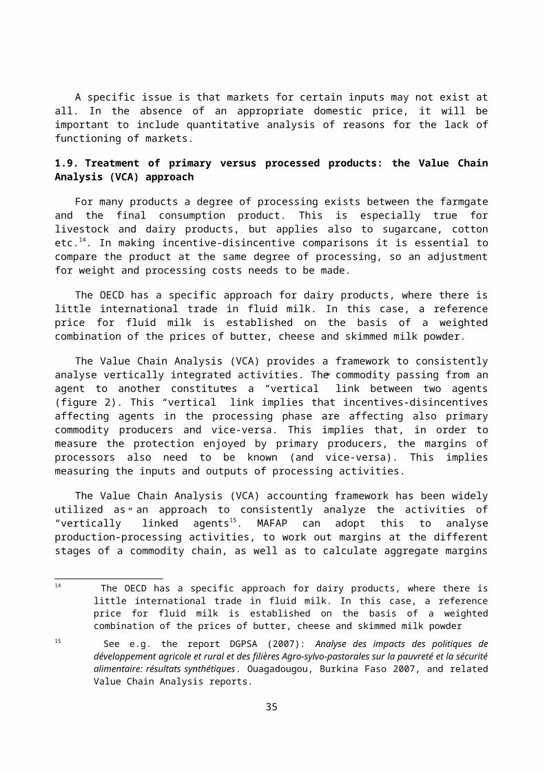
· school feeding programmes

· other

C. Payments to input suppliers

D. Payments to processors

E. Payments to traders

F. Payments to transporters

1.2. General sector support

Agricultural research

Technical assistance

Training

Extension/technology transfer

Inspection (veterinary/plant)

Infrastructure

· roads

· non-farm irrigation infrastructure

Storage/public stockholding

Marketing

Other

II. Agriculture supportive policies

Rural education

Rural health

Rural infrastructure

· roads

· water

· other

The proposed classification will be used for categorising all public expenditures regardless their source of financing (national budget or external aid). However, when classifying expenditures into these categories, each of them will be labelled with respect to the financing source (budget only, donor only or co-financed with adequate shares provided). Similarly, commodity information will be provided in a form of a label, distinguishing between programmes that are single, group or all commodities specific as appropriate.

Sector-specific and sector-supportive expenditures will be contrasted with non-agricultural expenditures. This will help to establish the importance of the sector in overall public expenditures and monitor progress towards the Maputo declaration 10% target. Further, the inclusion of rural expenditures in the “agriculture-supportive” category should demonstrate the extent to which there is a pro or anti-rural bias in areas such as infrastructure, health and education.

35

Discussion Question 2.1. Are these broad (inter-sectoral) and specific (within-sector) aspects of categorisation the most appropriate for quantifying expenditures in support of food and agriculture sector development?

The fisheries and forestry sectors will be treated separately to assure comparability of the indicators between countries. A similar classification is proposed for policies specific to these sectors (Box 2.2 and 2.3). Note that we are interested only in those aspects of the forestry sector that are linked to food sector.

Box 2.2. Proposed classification of public expenditures in support of the fisheries sector

I. Fisheries-specific policies.

1.1. Payments to the agents in the fisheries sector

A. Payments to producers

Direct payments

Input subsidies

Other

B. Payments to consumers

C. Payments to input suppliers

D. Payments to processors

E. Payments to traders

F. Payments to transporters

1.2. General sector support

Infrastructure

Education (training, extension etc.)

Research

Other

36

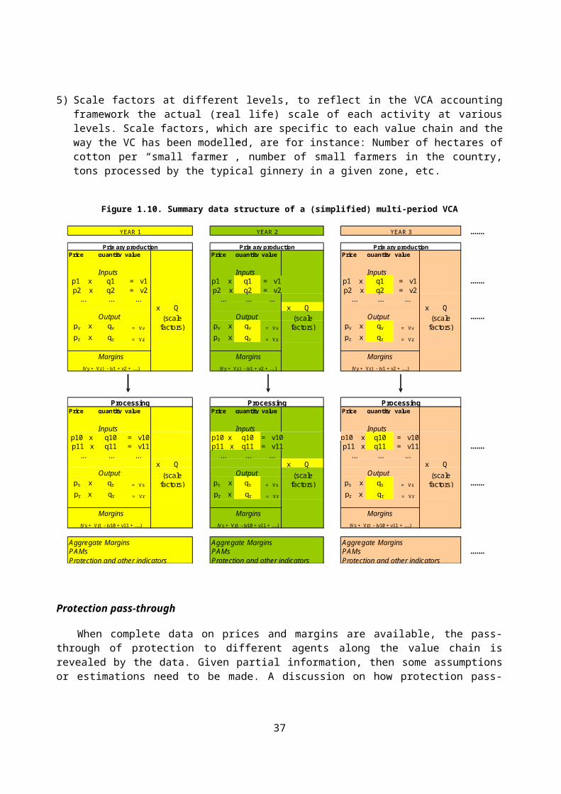
Box 2.3. Proposed classification of public expenditures in support of the forestry sector

I. Forestry-specific policies.

1.1. Payments to the agents in the forestry sector

A. Payments to producers

Direct payments

Input subsidies

Other

B. Payments to consumers

C. Payments to input suppliers

D. Payments to processors

E. Payments to traders

F. Payments to transporters

1.2. General sector support

Infrastructure

Education (training, extension etc.)

Research

Other

2.3. Definitions of categories

Precise definitions will be provided, following the example of the PSE Manual.

2.4. Complete coverage of institutions, administrative levels and financing instruments

It is important to identify all budgetary expenditures in support of the food and agriculture sector, regardless their source of financing – national or external aid. All financing through public institutions involved should be covered, considering the fact that implementation and funding of some relevant measures may occur outside the agricultural ministries. Further, funding from all administrative levels should be considered and many relevant policies may be financed at various levels of government (central, state, district, regional). Finally, all public finance instruments should be covered, regardless if they come from the regular budgets or are financed from some type of extra-budgets funds, that do not constitute part of the regular national budget and that are used for implementation of specific programmes.

2.5. Budgetary transfers versus revenue forgone

Monetary transfers in support of food and agriculture sector development may be provided in two forms: actual budgetary transfers (such as production subsidies) and the revenue forgone by the governments (such as administered prices for inputs – e.g. government buying fertiliser on international market and selling it to the farmers at a lower price – or tax concessions). Both types of transfers should be included in the calculations.

37

2.6. Mapping aid onto national expenditures

Figure 2.1. Mapping aid on national expenditures

commitments disbursements

• DAC bilateral• DAC multilateral• Other bilateral• Other multilateral

DONORS

• Central government• Local government• Specific projects conducted

by NGOs or international organisations

National budgets• Agriculture specificPayments to agents in

agro-food sectorGeneral sector support• Agriculture supportive

MAFAP public expenditure classification

budget actual spending

In order to capture all investments in the agro-food sector, the external aid information has to be taken into account. The aid relevant to the scope of the project can be provided in various forms and we need to assure that all are taken into account.

Figure 2.1 presents schematically mapping of aid on national expenditures. First, all donors need to be identified. These may be either “bilateral”, i.e. aid is provided by one donor country to the given recipient country, or “multilateral”, i.e. aid is provided via projects conducted by international organisations or international NGOs. We distinguish between Development Assistance Committee (DAC) donors and others, because of the available data sources. The information on the former will come from the Creditor Reporting System database of the OECD, while the latter will need to be collected based on the recipient’s information on sources of external aid. 22

Second, we will distinguish to the extent possible, between commitments and disbursements, using the latter to map on recipient’s budget. It is important to remember that commitments reflect donors’ programming and changes in their policies and hence they provide indication on the future flows, while disbursements provide information and actual spending. Consequently, commitments and disbursements are not directly comparable for the same year, as commitments for a given year will be disbursed over several subsequent years.

22 DAC members: Australia, Austria, Belgium, Canada, Denmark, European Commission, Finland, France, Germany, Greece, Ireland, Italy, Japan, Korea, Luxembourg, Norway, Netherlands, New Zealand, Portugal, Spain, Sweden, Switzerland, United Kingdom, United States. Multilateral donors included in the CRS database: World Bank, African Development Bank, Asian Development Bank, Inter American Development Bank, IFAD, UNICEF, other United Nations agencies.

38

As a next step we need to identify channels through which aid is provided: to the central government, to the local government or to specific projects conducted by NGOs, international organisations and other institutions. This information will be then linked with budgets reported by the recipient institutions. It is important to note that we will distinguish the three aforementioned channels only at an aggregate level to provide an overview of importance of each of the channels in providing aid. When classifying support measures into categories proposed in Box 2.1 we seek exclusively public expenditures and therefore we will consider only those aid programmes that are channelled through the government.

Recording aid flows at every step of its distribution will bring lots of valuable information. It will help to understand how effective donors are in disbursing the committed money. It will allow understanding if aid is provided for a specific purpose or it is in a form of general support to the budget. Finally, looking at the governments expenditures, it will be possible to see how much of the aid money was effectively spent as compared to the planned budget.

The CRS database provides information on aid by “sector” and “purpose code” (a subsector). The following table lists all agriculture specific categories. However, there are numerous other sectors or purpose codes that may be of relevance to agriculture and will need to be examined. For example, General Budget Support, once integrated in developing countries’ domestic budgets, will contribute to the development of the agricultural sector. The amounts relevant to agriculture cannot be precisely specified since support is of a general nature, without any specific use indicated, although it may be accompanied by various exclusions or understandings on the government’s development strategy, such as commitment to agriculture development. The exact numbers pertaining to agriculture, therefore, will need to be captured at the country level, analysing the state accounts.

Discussion Question 2.2. How complete is it possible / practical to be in reconciling aid flows with national expenditure data?

39

Table 2.1. CRS Agriculture-Specific Categories

Purpose code Description Notes on coverage31110 Agricultural policy and administrative

managementAgricultural sector policy, planning and programmes; aid to agricultural ministries; institution capacity building and advice; unspecified agriculture.

31120 Agricultural development Integrated projects; farm development.31130 Agricultural land resources Including soil degradation control; soil improvement;

drainage of water logged areas; soil desalination; agricultural land surveys; land reclamation; erosion control, desertification control.

31140 Agricultural water resources Irrigation, reservoirs, hydraulic structures, ground water exploitation for agricultural use.

31150 Agricultural inputs Supply of seeds, fertilizers, agricultural machinery/equipment.

31161 Food crop production Including grains (wheat, rice, barley, maize, rye, oats, millet, sorghum); horticulture; vegetables; fruit and berries; other annual and perennial crops.

31162 Industrial crops/export crops Including sugar; coffee, cocoa, tea; oil seeds, nuts, kernels; fibre crops; tobacco; rubber.

31163 Livestock Animal husbandry; animal feed aid.31164 Agrarian reform Including agricultural sector adjustment.31165 Agricultural alternative development Projects to reduce illicit drug cultivation through other

agricultural marketing and production opportunities.31166 Agricultural extension Non-formal training in agriculture.31181 Agricultural education/training31182 Agricultural research Plant breeding, physiology, genetic resources, ecology,

taxonomy, disease control, agricultural bio-technology; including livestock research (animal health, breeding and genetics, nutrition, physiology).

31191 Agricultural services Marketing policies & organisation; storage and transportation, creation of strategic reserves.

31192 Plant and post-harvest protection and pest control

Including integrated plant protection, biological plant protection activities, supply and management of agrochemicals, supply of pesticides, plant protection policy and legislation.

31193 Agricultural financial services Financial intermediaries for the agricultural sector including credit schemes; crop insurance.

31194 Agricultural co-operatives Including farmers’ organisations.31195 Livestock/veterinary services Animal health and management, genetic resources, feed

resources.Source: CRS database.

Overall, the following sectors are also being considered as potentially providing aid to agriculture:

· general budget support· trade policies and regulations· transport and storage· developmental food aid (but not emergency food aid)· rural development· agro-industry

40

· fertiliser (mineral and plant)· water supply and sanitation· forestry· fishing· support to non-governmental organisations

Table 2.2 at the end of this section provides full detail of sector and purpose codes mentioned above. In these particular sectors, elements linked to the food and agriculture sector will be included in the calculations.

The disaggregation in the CRS database is based on the general purpose of aid (hence the name “purpose code”) and does not reflect the different economic impacts that aid expenditures may have. For example, the support categories for agricultural development and for land and water resources are likely to range of subsidies and expenditures, some of which may be considered as public, but other will be clearly private and hence will have very different economic effects. Consequently, the CRS purpose codes only partially match the classification proposed here. They will need to be further disaggregated using the information on specific projects in order to map them onto our classification. This will be done using project description information available in the CRS database.

Data on non-DAC donors will need to be collected on a more ad-hoc basis. For each country main non-DAC donors will be identified as well as institutions disbursing the money. These institutions will be contacted to establish whether the data we seek are available.

Data needs and limitations section at the end of this section provides a more in-depth discussion on data sources.

2.7. Types of external aid

Donors provide aid either via both grants and loans. It is important to distinguish between these two types of aid as loans may have important impacts on the economy via the accumulation of debt and debt servicing requirements. Moreover, short-term loans on current expenditures have significantly different economic effects from longer-term loans for investment projects. The CRS database provides information on types of loans as well as on repayments periods and interest rates. However, it may be the case that loans are not reimbursed within given time-frame or not reimbursed at all, thereby contributing to debt accumulation. In some cases debts may be cancelled or partially written off. Hence, it is not clear a priori how much of a given amount of loans will effectively constitute loans with initially defined interest rates, how much will be re-scheduled and how much will de facto turn into grants. This type of information may be very difficult to obtain.

As a general approach, we propose to distinguish as far as possible between loans and grants using information available in the CRS database. Data on loans’ conditions, such as interest rates, repayment periods etc., should also be considered to keep track of potential pressures on the government’s budget that borrowing will cause. Additionally, information on overall level of loans will be collected to calculate a share of loans designated to the food and agriculture sector in the overall borrowing. This calculated share will be further used to estimate the share of the food and agriculture sector in overall debt and debt servicing (information on the latter can be obtained from relevant government bodies).

More in-depth analysis of types of loans at a disaggregated level may be considered in the country reports.

41

2.8. Budget planning versus actual spending

Ideally, for the public expenditures calculations we would always want to record the actual spending. Therefore, it will be important to collect the information on actual expenditures whenever possible. Budget data will be used only when actual expenditure data is not available. When estimations are done on the annual basis, it may be the case that the amounts effectively disbursed will not be available. In such case, budget allocations will be used as a proxy, which will be updated the following year to reflect the actual spending.

National budget planning and donor’s commitments will also be collected. This will allow comparison budget allocations and the actual spending to establish the efficiency of public expenditures (see below for details).

2.9. Treatment of policy administration costs

Administration costs include costs of formulation, implementation and evaluation of agricultural policies and generally should not be included in the calculations of support to the agro-food sector. This is because they represent the expenditures on operations and are not policy transfers as such. However, when support is provided via services, e.g. extension, training, research or inspection, expenses associated with deliver of the services, e.g. salaries of extension advisors, salaries of inspection officers or researchers, should be included the calculations.

The data on administration costs not included in the public expenditure calculations will be collected separately. It will make it possible to establish the shares of operational costs in overall government spending and contribute to the analysis of efficiency of public expenditures.

2.10. Treatment of one-off investments versus recurrent expenditures

Both investments and recurrent expenditures should be recorded on the annual basis using actual spending information. If the actual expenditures data are not available then budget allocations will need to be used instead, and the overall budget for a given investment will need to be allocated over time according to the investment implementation plan. Conceptually, it is similar to the commitments versus disbursements issue and should be handled in the same way.

It is important to note, however, that one-off investments have different economic impacts than recurrent expenditures. Although investments funds may be disbursed over relatively short time period, the benefits may be enjoyed over several consecutive years. In the public expenditure classification we are interested to record the actual year-to-year spending to analyse the government’s efforts in enhancing sector’s development and establish the progress towards the target of 10% sector’s share in overall public spending. However, when analysing the profitability of the investments, they will need to be allocated over time. Standard methods, such as net present value (NPV) may be employed to evaluate investments at hand.

2.11. Measuring efficacy, efficiency and effectiveness of public expenditures

Collecting information on monetary flows at different allocation levels, i.e. how much of a given budgetary allocation is actually spent, will shed some light on the efficacy of public spending. Tracking the flows will help to spot eventual leakages in the system and lack of efficacy in the use of resources by comparing budget allocations with actual spending.

The proposed classification will help to measure the efficiency of public expenditures in terms of whether and to what extent the pattern of expenditures is consistent with the government’s stated policy

42

objectives and policy needs. Moreover, analysing efficiency of expenditures financed by external aid may be of particular importance to donors, in helping them ensure that their support for specific projects is coherent with domestic policy objectives.

Although this is beyond of the scope of the project, it is important to note that collected information on public expenditures will also help to measure effectiveness of public expenditures. Because proposed classification is based on economic characteristics of support measure, it provides information on the first incidence of a given support measure. The latter, in turn, constitutes a good basis for further modelling work that can be conducted to investigate how effective the support measures are in meeting national development objectives. This includes partial equilibrium models such as the PEM and national and global general equilibrium models. In addition, econometric techniques can be employed to explore the effectiveness of various types of public expenditures such as agriculture, health, education, nutrition, infrastructure, research etc. in meeting objectives of economic growth and poverty reduction (Fan). A review of the uses of expenditure data is provided in the Synthesis Report.

2.12. Classifying support to the food and agriculture sector

Once all relevant items have been identified they will be classified into the categories provided in Box 2.1. It may happen, however, particularly for the more historical data, that the data reported is too aggregated to fit the classification proposed. For example, data may be presented by broad agricultural programmes composed of very heterogeneous elements. The attempt should be made to obtain the required disaggregation. If the desired disaggregated information is not available, then some estimation procedure may be applied, e.g. assumed percentage shares based on available data for other years or other, perhaps more qualitative, sources of information. For historical data, even the latter may not be possible. In such case, more aggregated categories will be considered, linked to the detailed classification for more recent time series. New data should be collected at the most disaggregated level possible.

2.13. Data needs and sources

1995 is proposed as a base year since the CRS database provides quality information only from that year onwards.

Data on national expenditures will be collected from budget accounts of the institutions identified as those providing or recording support to the food and agriculture sector. Data on aid flows from DAC members will come from the CRS database, while data on the other donors will be collected on an ad hoc basis.

The CRS database covers DAC members’ bilateral ODA i.e. activities undertaken directly with an aid recipient or with national and international non-governmental organisations active in development; and promotion of development awareness and other development-related spending in the donor country (e.g. debt reorganisation, administrative costs). DAC members’ multilateral aid, i.e. contributions to the regular budgets of the multilateral institutions is excluded.  However, projects executed by multilateral institutions or non-governmental organisations on behalf of DAC countries are included and classified as bilateral aid, because it is the donor country that effectively controls the use of the funds. Aid activities financed from the multilateral institutions’ regular budgets are referred to as “multilateral outflows”.

2.14. Information gaps

Generally, data may be weak except for the most recent years. For those years for which we will not be able to obtain sufficient disaggregation as suggested above, we will consider more aggregate items that will be mapped onto proposed detailed classification and disaggregation. Box 2.4 presents an example of an aggregated classification that would be used when data on national expenditures do not permit further disaggregation.

43

Box 2.4. Simplified classification for historical data

I. Agriculture-specific policies.

1.1. Payments to the agents in the agro-food sector

A. Payments to producers

Direct payments

Input subsidies

Other

B. Payments to consumers

C. Payments to input suppliers

D. Payments to processors

E. Payments to traders

F. Payments to transporters

1.2. General sector support

Infrastructure

Education (training, extension etc.)

Research

Other

II. Agriculture supportive policies

Rural education

Rural health

Rural infrastructure

As with national expenditures, data on aid may not be complete for more historical time-period. The proposed detailed classification and mapping of aid on national expenditures requires a good level of detail, which may not be available since 1995. In particular, we will need information on specific projects in order to disaggregate within the CRS purpose codes and information on aid distribution channels in order to identify recipient institutions, as explained above. The CRS database provides such information, however, it does not belong to the core information collected and, for the moment, it is provided on a voluntary basis. Inspection of that additional data reveals that quality information for MAFAP countries is available only for the most recent years. Older series will need to be complemented with the information on external aid we will obtain at the national level. For the future data collections, CRS will be able to provide the necessary detail - DAC donors have been requested to provide information on aid modalities (channels of distribution and project descriptions) on a regular basis starting 2010.

Further, data on the amounts disbursed each year are available at the activity level for some, but not all, donors. Data for years prior to 2002 provide disbursements only for 60% of database record. Preliminary analysis of disbursements information for the MAFAP countries showed that it is rather scattered. Moreover, for some donor-recipient pairs we have information only on commitments,

44

while for others only on disbursements and the desired distinction between the two may not be possible to achieve. We will then combine the two to provide an estimate of aid disbursements.

It is important to remember that the gap between disbursements and commitments may be significant (e.g. for years 2005-07). This is because commitments are followed by disbursements with a time lag, as explained above. If commitments are to be used as a proxy for missing disbursements information they will need to be allocated over the relevant years.

Discussion Question 2.3. Are the above proposals for addressing measurement issues the most appropriate?

45

Table 2.2. CRS sectors potentially relevant for agriculture

510 General budget support Budget support in the form of sector-wide approaches (SWAps) should be included in the respective sectors.

51010 General budget support Unearmarked contributions to the government budget; support for the implementation of macroeconomic reforms (structural adjustment programmes, poverty reduction strategies); general programme assistance (when not allocable by sector).

520 Developmental food aid/Food security assistance

52010 Food aid/Food securityprogrammes

Supply of edible human food under national or international programmes including transport costs; cash payments made for food supplies; project food aid and food aid for market sales when benefiting sector not specified; excluding emergency food aid.

920 SUPPORT TO NON- GOVERNMENTAL ORGANISATIONS (NGOs)

Official funds to be paid over to national and international private voluntary agencies for use at the latter’s discretion.

92010 Support to national NGOs In the donor country.

92020 Support to international NGOs

92030 Support to local and regional NGOs In the recipient country or region.

43040 Rural development Integrated rural development projects; e.g. regional development planning; promotion of decentralised and multi-sectoral competence for planning, co-ordination and management; implementation of regional development and measures (including natural reserve management); land management; land use planning; land settlement and resettlement activities [excluding resettlement of refugees and internally displaced persons (72010)]; functional integration of rural and urban areas; geographical information systems.

33110 Trade policy and administrative management

Trade policy and planning; support to ministries and departments responsible for trade policy; trade-related legislation and regulatory reforms; policy analysis and implementation of multilateral trade agreements e.g. technical barriers to trade and sanitary and phytosanitary measures (TBT/SPS) except at regional level (see 33130); mainstreaming trade in national development strategies (e.g. poverty reduction strategy papers); wholesale/retail trade; unspecified trade and trade promotion activities.

INDUSTRY32165 Fertilizer plants32161 Agro-industries Staple food processing, dairy products, slaughter

houses and equipment, meat and fish processing and preserving, oils/fats, sugar refineries, beverages/tobacco, animal feeds production.

312 FORESTRY

31210 Forestry policy and administrative management

Forestry sector policy, planning and programmes; institution capacity building and advice; forest surveys; unspecified forestry and agro-forestry activities.

31220 Forestry development Afforestation for industrial and rural consumption; exploitation and utilisation; erosion control,

46

desertification control; integrated forestry projects.31261 Fuelwood/charcoal Forestry development whose primary purpose is

production of fuelwood and charcoal.31281 Forestry education/training31282 Forestry research Including artificial regeneration, genetic improvement,

production methods, fertilizer, harvesting.31291 Forestry services

313 FISHING

31310 Fishing policy and administrative management

Fishing sector policy, planning and programmes; institution capacity building and advice; ocean and coastal fishing; marine and freshwater fish surveys and prospecting; fishing boats/equipment; unspecified fishing activities.

31320 Fishery development Exploitation and utilisation of fisheries; fish stock protection; aquaculture; integrated fishery projects.

31381 Fishery education/training31382 Fishery research Pilot fish culture; marine/freshwater biological research.31391 Fishery services Fishing harbours; fish markets; fishery transport and

cold storage. 210 TRANSPORT AND STORAGE Note: Manufacturing of transport equipment should

be included under code 32172.21010 Transport policy and administrative

managementTransport sector policy, planning and programmes; aid to transport ministries; institution capacity building and advice; unspecified transport; activities that combine road, rail, water and/or air transport.

21020 Road transport Road infrastructure, road vehicles; passenger road transport, motor passenger cars.

21030 Rail transport Rail infrastructure, rail equipment, locomotives, other rolling stock; including light rail (tram) and underground systems.

21040 Water transport Harbours and docks, harbour guidance systems, ships and boats; river and other inland water transport, inland barges and vessels.

21050 Air transport Airports, airport guidance systems, aeroplanes, aeroplane maintenance equipment.

21061 Storage Whether or not related to transportation.

21081 Education and training in transport and storage

140 WATER SUPPLY ANDSANITATION

14010 Water resources policy and administrative management

Water sector policy, planning and programmes; water legislation and management; institution capacity building and advice; water supply assessments and studies; groundwater, water quality and watershed studies; hydrogeology; excluding agricultural water resources (31140).

14015 Water resources protection Inland surface waters (rivers, lakes, etc.); conservation and rehabilitation of ground water; prevention of water contamination from agro-chemicals, industrial effluents.

14020 Water supply and sanitation - large systems

Water desalination plants; intakes, storage, treatment, pumping stations, conveyance and distribution systems; sewerage; domestic and industrial waste water treatment plants.

14030 Basic drinking water supply andbasic sanitation

Water supply and sanitation through low-cost technologies such as handpumps, spring catchment,

47

gravity-fed systems, rain water collection, storage tanks, small distribution systems; latrines, small-bore sewers, on-site disposal (septic tanks).

14040 River development Integrated river basin projects; river flow control; dams and reservoirs [excluding dams primarily for irrigation (31140) and hydropower (23065) and activities related to river transport (21040)].

14050 Waste management/disposal Municipal and industrial solid waste management, including hazardous and toxic waste; collection, disposal and treatment; landfill areas; composting and reuse.

14081 Education and training in water supply and sanitation

Source: CRS database.

48

PART 3. COUNTRY REPORTS AND DEVELOPMENT INDICATORS

3.1. Overview

The MAFAP country reports will contain a wide range of information. They w will draw on information on incentives/disincentives and public expenditures as laid out in previous sections. Performance and development indicators will complement country reports drawing principally from secondary sources. These will include (a) measures of performance in various domains, and (b) ancillary indicators relevant to interpreting the indicators on incentives/disincentives and public expenditures. For example indicator on percentage of rural roads paved will complement the analysis by linking the analysis of disincentives caused by (high) transportation costs and the government expenditures on infrastructure. This part will need to be elaborated in the context of an agreed table of contents for the country reports. Some of the indicators will be contextual, others will be used to complement directly the measures of incentives/disincentives and the analysis of government expenditures and will help better appreciate the progress made towards achieving policy outcomes.

The following sections present the domains for performance and development indicators and demonstrate how they will fit into a broad proposal of country report structure. Naturally country reports will contain a wide range of data, so it is helpful to make a distinction between core indicators that will be updated regularly as part of the project, and general statistics that will illuminate the reports.

Note that some indicators will not be neatly pigeon-holed into the report as below, as they may be relevant a various stages. For example, information on costs in output and input markets is helpful to understanding incentives and disincentives, but might also form part of a general description of market structures, and part of the discussion of whether government expenditures are being allocated to priority areas.

Discussion question: What should be the core set of performance and development indicators for all countries in the MAFAP project?

3.2. Coverage of proposed performance and development indicators

Information will be harnessed primarily from secondary sources, and coordinated with the CountrySTAT initiative to the extent possible. As far as possible, indicators already in use in the monitoring systems of participating countries, including the monitoring and evaluation system of the Comprehensive Africa Agriculture Development Programme (CAADP) would be used. Box 3.1. provides core indicators in the areas of interest. Other indicators will be considered in country reports based on specific needs.

49

Box 3.1. Coverage of proposed performance and development indicators

Sectoral performance

• Production, consumption, trade and changes in stocks. These figures will in any event need to be collected in order to compute policy distortions. In general, data are much easier to obtain for crops than for livestock products, which is a serious deficiency in many African economies.

Food production index (FAO-FAOSTAT) Food supply quantity tonnes, kg/capita/year; or grams/capita/day (FAO-FAOSTAT) Protein and fat supply quantity are given in grams/capita/day. (FAO-FAOSTAT) Food use (% annual change by commodity) (FAO-GIEWS) Opening stocks ( % annual change by commodity) (FAO-GIEWS) Prices of Principal Agricultural Trade Products (FAO-GIEWS) Trade Balance (FAO-GIEWS) Trade openness (% GDP, 1960-2005) (WTO) Share in the world total exports by main commodity group (WTO-CP) Share in the world total exports by main destination (WTO-CP) Share in the world total imports by main commodity group (WTO-CP) Share in the world total imports by main destination (WTO-CP) Indexes of Real Trade-Weighted LCU Exchange Rates (FMI-IFS) Agricultural Exports and Imports (WTO-CP) Agricultural Exports by Region (WTO-CP) Food exports (% of merchandise exports) (WTO-CP) Agricultural raw material exports (% of merchandise exports) (WB-WDI) Agricultural raw material imports (% of merchandise imports) (WB-WDI) Proportion (or ratio) of total value of agricultural sector exports to total agricultural sector value

added (FAO-FAOSTAT+ WTO-CP)• Crop yields, and value added as a share of livestock production

Change (percentage) in yields of major crops of the country (%) (FAO-GIEWS) Percentage increase in yield per livestock unit (%) (FAO-GIEWS) Annual growth in value added in the livestock sector (FAO-FAOSTAT) Capture fish production as a percentage of fish stock (FAO-FAOSTAT) Yield gap between farmers’ yields and on-station yields for major crops of the country (FAO-

NRC)• Productivity/efficiency of water use

Irrigation potential (1000 ha) (FAO-NRC) Area equipped for irrigation: equipped lowland areas (1000 ha) (FAO-NRC) Area equipped for spate irrigation (1000 ha) (FAO-NRC) Area equipped for irrigation: total (1000 ha) (FAO-NRC) Area equipped for irrigation: actually irrigated (1000 ha) (FAO-NRC)

• Agriculture as a share of rural and overall economic activity

Agriculture value added (% of GDP) (FAO-FAOSTAT) Annual growth (%) in agricultural value added (WB-WDI) Value of Agricultural Production (FAOSTAT) Annual growth of income from the agricultural sector (%) (WB-WDI) Employment in agriculture (% total of employment) (FAO-FAOSTAT) Agricultural land (% of land area) (FAO-TERRASTAT)

50

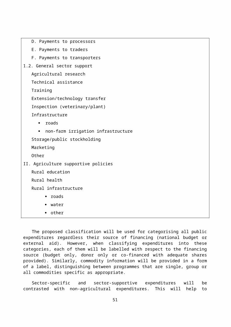
Poverty, inequality and food security

Poverty headcount ratio at national poverty line (% of population) (WDI) Percentage of population living below USD 1 a day (WDI) Gini Coefficient (IMF-IFS) GNI per capita, Atlas method (current US$) (WB-WDI) Rural relative to urban per capita incomes (WB-WDI) Malnutrition prevalence, weight for age (% of children under 5) (WDI) Proportion on undernourished population (%) (FAO-FAOSTAT Proportion on undernourished women in the population Share of urban households which are food insecure; share of rural / farm households that are

food insecure. (FAO-RIGA)

Costs in output markets

Mobile cellular subscriptions in rural areas (per 100 people) (WB-WDI) Extent of rural electrification (WB-WDI) Change (percentage) in unit cost of transportation of agricultural products (%) (WB-WDI) Percentage of road paved

Costs in input markets

Proportion of land area formally established as a protected area (%) (WB-WDI) Land area for which there is a legally recognized form of land tenure (%) (FAO-TERRASTAT) Percentage of land area for which there is a legally recognized form of land tenure (%) (FAO-

TERRASTAT) Percentage of agricultural households that have legally recognized rights to land (%) (FAO-

TERRASTAT) (disaggregated by gender) Percentage change in number of formal land transactions (quarterly or yearly basis) (%) (FAO-

TERRASTAT) Area equipped for irrigation: equipped lowland areas (1000 ha) (FAO-NRD and CountrySTAT) % Change in access to formal credit (WB-WDI) % of the rural population using financial services of formal banking institutions (%) Recovery rate of rural credit (%) (WB-WDI) % change in Agricultural credit, 1990-2006 (WD-WDI)

Environment and natural resources

Improved water source, rural (% of rural population with access) (FAO-FAOSTAT) Aggregated mineral fertilizer use and equiv per ha (FAO-FAOSTAT) Aggregated pesticide use and equiv per ha (FAO-FAOSTAT) Aggregated estimated water consumed for irrigation (FAO-FAOSTAT) Rate of deforestation (percentage) (FAO-COUNTRYSTAT) Proportion (percentage) of land area covered by forest (FAO-COUNTRYSTAT) Ratio (or proportion) of arable land area to total land area of the country (WB-WDI) Degree of deforestation (% of deforested land, or yearly deforested areas) (WB-WDI) Soil carbon capital, e.g. soil carbon per ha (WB-WDI) 0-30 cm Soil Carbon volume per country (FAO-NRC) Improved water source, rural (% of rural population with access) (WB-WDI)

51

Health and human development

Mortality rates , under -5 (per 1,000) (WB-WDI) Life expectancy at birds (total years) (WB-WDI) Prevalence of HIV, total (% of population ages 15-49) (WB-WDI) Fertility rates, total (births per woman) (WB-WDI) School enrollment, secondary (% gross) (WB-WDI) School enrollment, secondary (% net) (WB-WDI) Long-term unemployment, female (% of female unemployment) Labor force, female (% of total labor force) (WB-WDI)

Market structures

Change (percentage) in yields of major crops of the country (%) (FAO-GIEWS) Percentage increase in yield per livestock unit (%) (FAO-GIEWS) Annual growth in value added in the livestock sector (FAO-FAOSTAT) Capture fish production as a percentage of fish stock (FAO-FAOSTAT) Output indices for crop and livestock products, 1990 = 100 (FAO-FAOSTAT) Real wholesale price indexes for main agricultural commodities, 1990 = 100 (FAO-FAOSTAT) Yields for selected crops, 1990-2005 (1990 = 100) (FAO-FAOSTAT) Evolution of employment in agriculture, 1990-2006 (ILO-LABORSTAT) Labour productivity by sector (value added per employee, 1986 = 100) (ILO-LABORSTAT)

3.3. Proposed structure of country reports

The core indicators presented in Box 3.1. will feed into the country reports. Box 3.2. presents a proposed sample structure of a country report and shows how performance and development indicators would fit into it (by broad area as set out in Box 3.1.).

Box 3.2. Proposed structure of country reports

HIGHLIGHTS AND POLICY RECOMMENDATIONS

One page summary of key data and indicators (standard for all countries)

I. THE POLICY CONTEXT

This section will examine key issues that have shaped developments in the agro-food sector and conditioned policy responses.

A. General aspects

Background information on the national economy. Example coverage: (population, GDP/income per caput, trade balance, poverty, food security). Social and political environment and its evolution (political parties, CSOs in food and agriculture, private sector, development partners and other stakeholders). Changes in the macroeconomic environment and its effects (exchange rate, inflation rate, interest rate, debt, budget and fiscal policy). External commitments (global or regional agreements and conventions)

Performance and development Indicators:

Poverty, inequality and food security

52

Health and human development

B. Agricultural Situation

Descriptive information

Performance and development Indicators:

Sectoral performance

Market structures

Environment and natural resources

C. Structural change in the agro-food sector

Land policy and farm restructuring. Competitiveness and structural change in the upstream and downstream sectors (legal framework; supply and service enterprise; processing enterprises; wholesaling and retailing enterprises; foreign-trade enterprises)

II. POLICY TRENDS

This section will introduce the MAFAP methodology of measurement of incentives and disincentives in place for key value chains and their evolution over time, making distinction between those induced by formal policies and those resulting from other factors (high costs, rents, imperfect pass-through of price changes, and others) and present historical data for the country. The specific policies underlying these numbers will then be evaluated. Recent changes in policies will be highlighted (what is our reference period for this?)

A. Agricultural policy framework

Agricultural policy objectives; Basic steps in agricultural policy reform; Basic policy instruments; Institutional arrangements for administering policy

B. Domestic policies

Price and income support measures; Reduction of input costs (credit policies, input subsidies, tax policy); Rural public services infrastructure (research and development, education and training, quality and sanitary control, agricultural infrastructure, marketing and promotion); Consumer measures; Environmental measures; Overall budgetary outlays on agro-food policies; “missing policies” as identified on the basis of non-formal policy related incentives/disincentives

C. Trade policies

Trade flows (composition of agro-food trade; destination and origin of agro-food trade); Trade relations (bilateral, regional and multilateral agreements and their impact on trade flows); Tariff and non-tariff measures applied by the country's main trading partners and their impact on its agro-food exports;

53

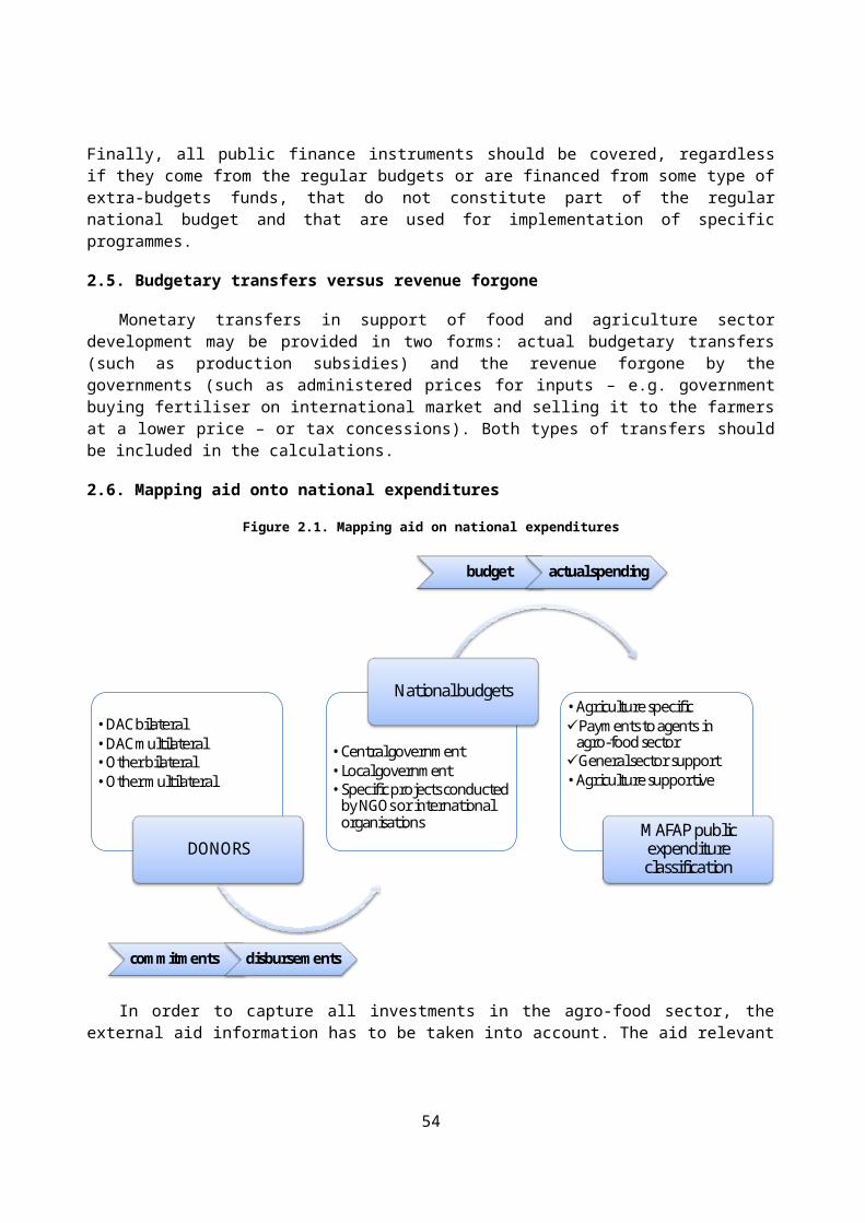
Trade policy measures

D. Monitoring of incentive/disincentives to agriculture

Information from Part 1.

· Aggregate results

· Decomposition analysis (including distributional effects)

· Focus on key value chains and decomposition into formal policy and other sources of incentive/disincentive

Performance and development Indicators:

Costs in output markets

Costs in input markets

E. Monitoring of government expenditures in support of food and agriculture sector development

Information from Part 2 plus interpretation.

III. POLICY ISSUES

This section will focus on issues of particular interest for the Government. While the issue addressed must be related to agriculture, it could include, for example, links to related policy objectives (e.g. labour/land reforms; environmental goals; poverty reduction; rural development), analysis of policy reform scenarios (e.g. agriculture or trade; domestic, regional or multilateral reforms) and/or distributional questions (e.g. household level impacts, consumers vs. producer welfare gains, commercial and small farms impacts).

Notes and references

Bibliography

ANNEX 1. Agricultural policies and support for individual commodities

Final commodity coverage will need to be discussed and agreed with the country experts and will depend on the importance of a given product and data availability, but basic commodities could include the following: wheat, maize, rice, other grains, soybeans, rapeseeds, peanuts, sugar (cane and/or sugar beet), cotton, potatoes, apples, oranges, tobacco, milk, beef, pork, sheep meat, poultry meat, and eggs.

ANNEX 2. MAFAP methodology and calculations

54

ANNEX 1. POLICY DISTORTIONS AND THE “DEVELOPMENT GAP” IN GHANA

The following examples for Ghana, one of the countries covered by the DAI project, demonstrate the scope for decomposing price gaps along the value chain in order to distinguish between explicit, policy-induced, price incentives and disincentives on the one hand, and excessive costs and rents on the other, which can be considered as a “development gap”. The information here draws on the Ghana study in the DAI project, and considers three products: the country’s main export (cocoa) and its two main food imports (rice and maize).

In the case of cocoa, data exist on the f.o.b. export price, the producer price and on export taxes paid to the Treasury. The difference between the f.o.b. price and the price paid to producers plus the export tax represents money that is retained by the government’s marketing board COCOBOD. Historically, the sector was heavily mismanaged, and only a minor share of the export price was returned to the producer (Figure A.1, Panel A). Reforms to COCOBOD gathered momentum after the 1992 civilian elections. Major changes introduced were a reduction in staff levels from over 100,000 in the early 1980s to 10,400 in 1995 and just over 5,100 staff by 2003; an end to input marketing; and the introduction of competition into internal marketing.

There was some reduction in COCOBOD’s share of export earnings in the 1990s, but as cocoa prices have strengthened in recent years that share has risen again. Export tax payments made by COCOBOD to the government declined from an average of 40-50% of FOB earnings during the mid 1990s to less than 10% by 2004. As prices have risen, however, COCOBOD has increased its retained share of the export price, with the result that there has been a much milder reduction in the implicit taxation of the Ghanaian producer. (Figure A.1).

It is difficult to measure the “efficient” level of costs that should be absorbed by COCOBOD, although the minimum share taken offers a guide. On a conservative assumption that 25% of the f.o.b. price would be retained by COCOBOD to administer its legitimate marketing and other functions (implicit in Figure C.1), a large amount is still being retained and constitutes an informal tax on the Ghanaian producer – a kind of development gap. A task of MAFAP would be to split out the rent plus cost figure in Figure C.2 in a less arbitrary way.

55

Figure C.1. Allocation of the f.o.b. export price for cocoa beans, 1955-2004

Allocation of FOB Export Price, Cocoa

0

500

1000

1500

2000

2500

3000

3500

4000

1955

1957

1959

1961

1963

1965

1967

1969

1971

1973

1975

1977

1979

1981

1983

1985

1987

1989

1991

1993

1995

1997

1999

2001

2003

Rent + Export TaxMarketing Board costsProducer price

Figure C.2. Allocation of FOB export price, based on data on export tax payments in the 1990s

-

200

400

600

800

1 000

1 200

1 400

1 600

1 800

2 000

US d

olla

rs p

er to

nne

Rent plus cost

Export tax

Producer price

Source: COCOBOD.

56

Note that the export tax is calculated by dividing COCOBOD payments by the number of tonnes produced that year. The timing of payments may not correspond to the precise dates for which duties were applicable, so the series may not be perfectly comparable with the two price series.

In the case of rice and maize, domestic prices are available at the wholesale level. These prices are compared with landed c.i.f. values, which are adjusted for port charges, internal transport costs and quality differences in order to arrive at the NRA. In each case, it is assumed that processing and handling charges are of the same proportion for both domestic and imported products, such that the NRA at the wholesale level is equal to the NRA at the farmgate level. The aim of ADPI would be to relax these assumptions.

Prior to the mid-1980s, rice producers received less than the imported price (reported at the farm-gate) suggesting implicit taxation, while maize producer prices were at a similar level to imported prices (again compared at the farm-gate) (Figure C.3, Panel A; Figure C.4, Panel A). In both cases, domestic prices increased sharply in the mid-1980s, but the degree of price protection to producers has since diminished to levels somewhat higher than the statutory import tariff of 20% (Figure C.3, Panel B; Figure C.4, Panel B). This implies that the residual of the price gap, once known costs are accounted for, is higher than the tariff. Here this is attributed to additional protection, although there could also be unobserved “behind-the-border” costs.

Survey data exist on the costs of production and marketing for each commodity, although a time series was not available. These data were used to estimate NRAs at the wholesale level, with the simplifying assumption that pass-through to the farmer is 100%. The level of cost used to make the wholesale price adjustment is the actual cost of getting the product from the biggest wholesale market to the border. The survey data contain enough information to calculate (a) different levels of cost for shipping from different locations, and potentially the excess cost to Ghanaian producers as compared with the minimum cost per unit distance; and (b) variations in farm-wholesale margins. If one assumes that the lowest margin is “efficient”, this would provide a crude estimate of the excess farm-wholesale margin faced by Ghanaian producers.

To summarise, instead of estimating one NRA for each commodity, and assuming that the NRA at the wholesale level is equal to the NRA at the farmgate level, it should be possible to extract four numbers: NRAs at the farm and wholesale level, and excess costs (the “development gap”) at each level.

57

Figure A.3. Rice prices

Rice prices, US dollars per MT

0

500

1000

1500

2000

2500

1961

1963

1965

1967

1969

1971

1973

1975

1977

1979

1981

1983

1985

1987

1989

1991

1993

1995

1997

1999

2001

2003

Thai export priceBorder price farmgateWholesale priceProducer price

RICE PRICES cedis / MT

-

500,000

1,000,000

1,500,000

2,000,000

2,500,000

3,000,000

3,500,000

4,000,000

4,500,000

1985 1986 1987 1988 1989 1990 1991 1992 1993 1994 1995 1996 1997 1998 1999 2000 2001 2002 2003 2004

FarmgatepriceWholesalepriceBorder price

58

Figure A.4. Maize prices

Maize prices, US dollars per MT

0

200

400

600

800

1000

1200

1400

1600

1955

1957

1959

1961

1963

1965

1967

1969

1971

1973

1975

1977

1979

1981

1983

1985

1987

1989

1991

1993

1995

1997

1999

2001

2003

Wholesale priceProducer priceCIF import price

MAIZE PRICES cedis / MT

-

500,000

1,000,000

1,500,000

2,000,000

2,500,000

1985 1986 1987 1988 1989 1990 1991 1992 1993 1994 1995 1996 1997 1998 1999 2000 2001 2002 2003 2004

Wholesale price

Farmgate price

Border price(farmgate)

59

ANNEX 2. PRICE DECOMPOSITIONS FOR EXPORTABLE, IMPORTABLE AND NON-TRADABLE

Exported productExample: Gum Arabic in Burkina Faso

Unit:cfa/ton 2007a Benchmark price (FOB, €) 818b Official Exchange Rate 500c Premium 1d=a*b Border price (Official) 409000d'=a*b*c Border (Shadow) 409000e per unit export tax 0f export tax rate (ad valorem tax) 0.00%g=d'*f+ e export tax 0h=d'+g Shipped Border+ Tariff 409000

i Observed Transaction Costs Efficient and/or Excessive costs of: transport, handling, storage, margins 37.65

j Adj.factor for transaction Costs 0.8

k=i*j Efficient Transaction Costs from border to wholesale 30.12l=i-k Excessive transaction Costs 8m Externalities 0n Observed wholesale 450000o Adj.quality 1p= n*o Adjusted observed wholesale price 450000q= d'+k Reference price wholesale market level BP+ efficient transaction costs 408970

A Observed Transaction costs from farm to wholesale 2B adj factor for transaction costs 0.6C=A*B Efficient Transaction Costs 1.2D=A-C Excessive Transaction Costs 0.8I Producer Tax (-) or subsidy(+) -2L Reference Price at Farm gate level 408969M Observed farm gate (paid) price 449998N Observed farm gate (received) price 449996

INDICATORStw= p-q TOTAL WEDGE 41030

mdg= tw-bpw MARKET DEVELOPMENT GAP 41030pw= g POLICY WEDGE 0nri=(p-q)/q Nominal Rate of Incentive 0.10nrp=(p-(p-pw))/(p-pw) Nominal rate of protection 0

nrsd= (o-(o-mdg)/(o-mdg)Nominal rate of structural disincentive(development gap) 0.10

TW=N-L TOTAL WEDGE 41027

MDG= TW-PW MARKET DEVELOPMENT GAP 41029PW=I POLICY WEDGE -2NRI= (N-L)/L Nominal Rate of Incentive 0.10NRP=(N-(N-PW)/(N-PW) Nominal Rate of Protection -0.000004

NRSD=(N-(N-MDG)/(N-MDG)Nominal rate of structural disincentive 0.10

FARMGATE LEVEL

ABSOLUTE VALUES

RATES

WHOLESALE LEVEL

FARMGATE LEVEL

WHOLESALE LEVEL

ABSOLUTE VALUES

RATES

60

Imported productExample: Tilapia Fish in Burkina Faso

Unit:cfa/kg 2006a Benchmark price (CIF, €) 2b Official Exchange Rate 500c Premium 1d=a*b Border price (Official) 1000d'=a*b*c Border (Shadow) 1000e per unit tariff 0f tariff rate (ad valorem tariff) 26.85%g=d'*f+ e tariff 268.5h=d'+g Landed Border+ Tariff 1268.5

i Observed Transaction Costs

Efficient and/or Excessive costs of: transport, handling, storage, margins 378

j Adj.factor for transaction Costs 1k=i*j Efficient Transaction Costs from border to wholesale 378l=i-k Excessive transaction Costs 0m Externalities 0n Observed wholesale 1750o Adj.quality 1p= n*o Adjusted observed wholesale price 1750q= d'+k Reference price wholesale market level BP+ efficient transaction costs 1378

A Observed Transaction costs from farm to wholesale 504B adj factor for transaction costs 0.9C=A*B Efficient Transaction Costs 453.6D=A-C Excessive Transaction Costs 50.4I Producer Tax (-) or subsidy(+) 0L Reference Price at Farm gate level 924M Observed farm gate (paid) price 1246N Observed farm gate (received) price 1246

INDICATORStw= p-q TOTAL WEDGE 372

mdg= tw-bpwMARKET DEVELOPMENT GAP 104

pw= g POLICY WEDGE 269nri=(p-q)/q Nominal Rate of Incentive 0.27nrp=(p-(p-pw))/(p-pw) Nominal rate of protection 0.18

nrsd= (o-(o-mdg)/(o-mdg)

Nominal rate of structural disincentive(development gap) 0.06

INDICATORSTW=N-L TOTAL WEDGE 322

MDG= TW-PWMARKET DEVELOPMENT GAP 322

PW=I POLICY WEDGE 0NRI= (N-L)/L Nominal Rate of Incentive 0.35NRP=(N-(N-PW)/(N-PW) Nominal Rate of Protection 0.00

NRSD=(N-(N-MDG)/(N-MDG)Nominal rate of structural disincentive 0.35

FARMGATE LEVEL

ABSOLUTE VALUES

RATES

WHOLESALE LEVEL FARMGATE LEVEL

WHOLESALE LEVEL

ABSOLUTE VALUES

RATES

61

Non Traded productExample: Firewood in Burkina Faso

(SUBSTITUTE: IMPORTED BUTANE GAS)

Unit:cfa/kg 2007

a Benchmark price (CIF OF SUBSTITUTE, €)This price can be the CIF price of an imported substitute, the price of a local substitute or an implicit price based on shadow factor prices 0.65

b Official Exchange Rate 500c Premium 1d=a*b Border price (Official) 325d'=a*b*c Border (Shadow) 325e per unit tariff 0f tariff rate (ad valorem tariff) 0.00%g=d'*f+ e tariff 0h=d'+g Landed Border+ Tariff 325

i Observed Transaction Costs Efficient and/or Excessive costs of: transport, handling, storage, margins 272

j Adj.factor for transaction Costs 0.8

k=i*jEfficient Transaction Costs from border to wholesale 217.60

l=i-k Excessive transaction Costs 54m Externalities 0n Observed wholesale 115o Adj.quality 3p= n*o Adjusted observed wholesale price 345q= d'+k Reference price wholesale market level BP+ efficient transaction costs 543

AObserved Transaction costs from farm to wholesale 16

B adj factor for transaction costs 0.9C=A*B Efficient Transaction Costs 14.4D=A-C Excessive Transaction Costs 1.6I Producer Tax (-) or subsidy(+) -50

L Reference Price at Farm gate level 528M Observed farm gate (paid) price 329

N Observed farm gate (received) price 279

INDICATORStw= p-q TOTAL WEDGE -198

mdg= tw-bpw MARKET DEVELOPMENT GAP -198pw= g POLICY WEDGE 0nri=(p-q)/q Nominal Rate of Incentive -0.36nrp=(p-(p-pw))/(p-pw) Nominal rate of protection 0.00

nrsd= (o-(o-mdg)/(o-mdg)Nominal rate of structural disincentive(development gap) -0.36

TW=N-L TOTAL WEDGE -249

MDG= TW-PW MARKET DEVELOPMENT GAP -199PW=I POLICY WEDGE -50NRI= (N-L)/L Nominal Rate of Incentive -0.47NRP=(N-(N-PW)/(N-PW) Nominal Rate of Protection -0.15

NRSD=(N-(N-MDG)/(N-MDG)Nominal rate of structural disincentive -0.42

FARMGATE LEVEL

ABSOLUTE VALUES

RATES

WHOLESALE LEVEL FARMGATE LEVEL

WHOLESALE LEVEL

ABSOLUTE VALUES

RATES

62

NOTE 1:

The following names have been consistently employed to designate different items:

· Reference price indicates the CIF price for imported products, the FOB for exported products; a substitute for or an implicit price for products which are not traded internationally.

· Border price indicates the benchmark price translated into local currency; this corresponds to Pw in figures 1.3 to 1.5.

· Landed price indicates the border price plus tariffs or taxes; this corresponds to Pw(1+t) in figures 1.3 to 1.5..

· Observed price indicates the price observed in domestic markets; this corresponds to Pd in the main text.

· Adjusted Reference price indicates the border price plus normal (efficient) marketing costs up to the wholesale or farm gate level; this corresponds to Pw (1+t) ± T0 ± T1 in figures 1.3 to 1.5.

· Nominal Rate of Protection is the difference between observed price and the adjusted reference price (that is, the reference price adjusted by the cost of bringing it to the point of competition with the domestic commodity), as a fraction of the adjusted reference price. NRP = Pd – (Pb +T)/(Pb+ T)

· Nominal Rate of Assistance is the unit value of production at observed price less its value at the adjusted reference price plus the value of direct subsidies per unit of output, expressed as a fraction of the adjusted reference price. NRA = Pd – (Pb +T +S)/ (Pb + T +S)

· Effective Rate of Protection is the unit value added at observed price less its value at the adjusted reference price (where value added is the value of output minus the unit cost of traded intermediate inputs).

· Effective Rate of Assistance is the unit value added at observed price less its value at the adjusted reference price plus the value of direct subsidies per unit of output and intermediate inputs.

· Relative Rate of Assistance is the nominal rate of assistance to agriculture relative to the nominal rate of assistance to non-agricultural activities. RRAag = [(1 + NRAag)/(1+ NRAnon-ag) – 1]

· Trade Restrictiveness Index is the uniform import tariff rate which, if applied to all countries in place of all actual price distortions, would result in the same reduction in the volume of imports as the actual distortions.

· Market Development Gap is the sum of the excessive costs arising from inefficiencies and those arising from monopolistic/monopsonistic rents. This is equivalent to the difference between the observed price and the adjusted reference price plus the policy wedge.

· Nominal Rate of Structural Disincentive is the difference between the observed price and the adjusted reference price plus the policy wedge, as a fraction of the adjusted reference price plus the policy wedge. This is equivalent to ration of the Market Development Gap to the adjusted reference price plus the policy wedge.

NOTE 2:

The first two examples are quite straightforward. They refer to products which are imported or exported, for which a domestic close substitute is readily available. The assumption for these products is that the differences between the internationally traded and the domestically produced goods may be accounted for by adjustment coefficients.

The third example refers to products which are not traded internationally; treatment is pretty similar to the one for imported and exported products. The main difference is in the benchmark price, where credible information needs to be inserted.

63

ANNEX 3. BEYOND THE BORDER EFFECTS

We maintain here the same money metric as before to measure the incentive/disincentive on producer as determined, this time, also by the excess beyond-the-border costs and rents. We consider two countries, the one exporting a commodity (country A) and the one importing it (country B). Let’s consider the farmgate price for the exported commodity in country A:

(1)

where is the FOB price in foreign currency, ER is the exchange rate (units of domestic currency for one unit of foreign currency), S is the “unit” export subsidy (negative when a tax), is the “efficient”

component of costs incurred to take the commodity from the producer to the border and represents “excessive” costs incurred to take the commodity from the producer to the border. .represents the rent claimed by the downstream agent at the expense of the domestic producer. So far, we are considering what happens within country A. However, the final consumers of the commodity are located in country B, where the retail domestic price is:

(2)

CIF is the international “Cost, Insurance, Freight” incurred to take the commodity from country A to country B, TA is the import tariff applied in country B, is the “efficient” component of costs incurred

to take the commodity from the border to the retail market and represents “excessive” costs incurred to cover the same distance. represents the rents from the border to the retail market.

Rearranging terms in (2) gives the FOB price:

(3)

The farmgate price in country A is now obtained as determined by excess costs and rents within the destination country B by replacing (3) in (1):

(4)

64

ANNEX 4: PROTECTION PASS THROUGH ALONG VALUE CHAINS

Does a protection measure, such as a tariff, affect all agents of a given value chain equally? And does a protection measure over one agent of a value chain, such as a subsidy, spread proportionally over all other agents operating in the same value chain? In this paragraph, we briefly describe how this kind of questions is addressed in the OECD methodology and in the VCA/PAM methodology and highlight some open questions regarding this issue.

OECD Methodology The OECD methodology, as expounded in the PSE Manual, suggests that the price gap between the domestic market price and the reference price be computed for a given level of the value chain (i.e., farm gate). Then the price gap for another level can be derived either by: (i) assuming that the price gap measured at another level of the value chain (i.e. wholesale) is the same in absolute values, or by (ii) computing a “rate of protection” and assuming that it is the same at all levels of the value chain. The basic idea of latter method is that rather than inducing the same “absolute” price differential, policies affect all agents operating in the chain in the same “degree” or “proportion”. This assumption can be made when the assumption of competitive markets is made, but proves inaccurate when the competitive markets assumption is removed.

VCA/PAM Methodology In the VCA/PAM methodology, the price gap between the domestic market price and the reference price is computed at farm gate and wholesale level by using data collected at both levels, and no assumption is made on the transmission mechanisms of protection from an upstream to a downstream agent. The reference price of traded commodities is computed on the basis border prices, while for non- traded commodities the computation is done on the basis of input opportunity costs. The non-traded commodity enters as an input in the calculation of the PAM of the traded commodity, following a quite common assumption in VCA/PAM methodology, i.e. that the cost of the non-traded commodity is split into its tradable and non-tradable components, as it results from the PAM of the non-traded commodity. However, while this assumption is consistent with the other assumptions adopted to build PAMs, it may hide some shifts of protection between the downstream (traded) and the upstream (non-traded) commodity. In other words, when an agent passes on some protection to another agent in the value chain, this transfer is captured only to some extent by standard VCA/PAM indicators such as the Effective Protection Coefficient (EPC). Let’s show this through an example.

Example of protection pass-through in the VCA/PAM methodology Let’s take the value chain of sugar and consider two types of agents in the value chain: sugarcane producer and sugar producer. We compute a PAM for each of the two agents, adopting a quite common assumption VCA/PAM methodology, i.e. that the cost of sugarcane enters the PAM of the sugar producer (sugarcane being one of the inputs of sugar production) split into its tradable and non-tradable components, as it results from the PAM of the sugarcane producer. The two PAMs are the following:

Figure 3. Policy Analysis Matrix -baseline situation

A. Sugarcane producer B. Sugar producer

65

  REVENUES

COSTS

PROFITSTradable

InputsDomesticFactors &Not traded

inputs

Market Prices 120 30 80 10

SocialPrices 110 40 70 0

Gap 10 -10 10 10

  REVENUES

COSTS

PROFITSTradable Inputs

DomesticFactors &

Not traded inputs

Market Prices 1000 200+30=

230500+80+10=

590 180

SocialPrices 800 200+40=

240500+70=

570 -10

Gap 200 -10 20 190

The numbers in blue colour derive from the PAM of the sugarcane producer.

Panel A and B of Figure 3 show that sugarcane producer and sugar producer enjoy both higher revenues and higher profits than what they would enjoy in a perfect competition and no policy situation. This is due to the fact that domestic market prices are higher then the social values of both sugarcane and sugar.

Now, suppose that, all other thing staying equal, sugarcane producer is able to sell sugarcane to the sugar producer at a higher price (i.e., 130), thus reducing the profits that the sugar producer is making because of the policies in place/ existing market distortions (=supernormal profits). We call this situation: “alternative scenario”. We build a PAM for the two agents under this new scenario (Figure 4) and compute the Effective Protection Coefficient (EPC)23 (Figure 5). The EPC of the sugarcane producer in the alternative scenario is higher than that in the baseline situation, because part of the protection of the sugar producer has been transferred to the sugarcane producer. Surprisingly enough, this same transfer is not captured by the EPC of the sugar producer, which in turn stays unchanged, even though the supernormal profits of the sugar producer have decreased.

A more accurate indicator is what in the PAM literature is called the Benefit Cost Ratio24, which can be computed at both market and reference prices. As shown in Figure 6, these indicators increase in the alternative scenario for the sugarcane producer and decreases for the sugar producer, thus capturing that the supernormal profits of the sugarcane producer increase at the expenses of the supernormal profits of the sugar producer.

Figure 4. Policy Analysis Matrix –alternative scenario

A. Sugarcane producer B. Sugar producer

  REVENUES

COSTS

PROFITSTradable

InputsDomesticFactors &Not traded

inputs

Market Prices 130 30 80 20

SocialPrices 110 40 70 0

Gap 20 -10 10 20

Figure 5. Effective Protection Coefficients: Summary table

SUGARCANE PRODUCER

SUGAR PRODUCER

CONSOLIDATED VALUE CHAIN

BASELINE SCENARIO 1.29 1.37 1.37

ALTERNATIVESCENARIO-1 1.43 1.37 1.37

23 Note that the EPC is computed as (A-B)/(E-F).24 The Benefit Cost ratio is computed as A/(B+C) at market prices and as E/(F+G) at reference prices.

66

  REVENUES

COSTS

PROFITSTradable Inputs

DomesticFactors &

Not traded inputs

Market Prices 1000 200+30=

230500+80+20=

590 170

SocialPrices 800 200+40=

240500+70=

570 -10

Gap 200 -10 30 180

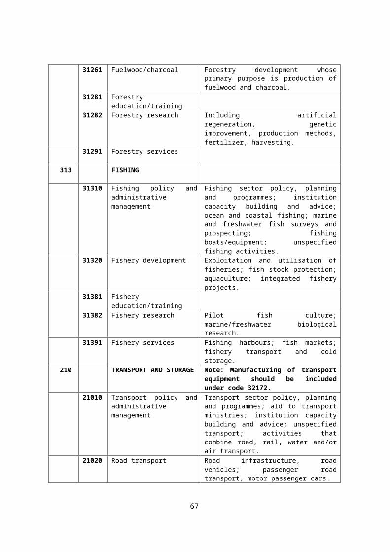
Figure 6. Benefit- Cost Ratio at observed market and reference prices

SUGARCANE PRODUCER SUGAR PRODUCERBaseline scenario

Alternative Scenario

Baseline scenario

Alternative Scenario

A/B+C 1.09 1.18 1.21 1.20E/F+G 1 1 0.98 0.98(A/B+C)/( E/F+G) 1.09 1.18 1.21 1.20

We suggest that within MAFAP, the EPC be computed to capture the protection of the consolidated value chain. In addition, indicators such as the Benefit-Cost Ratio –BCR, could also be worked out, as they capture how protection spreads over agents (changing their profitability).

67