THE WORLD BANK ECONOMIC REVIEW, VOL. 14, NO. 2. 287-307

Monitoring Banking Sector Fragility:A Multivariate Logit Approach

Ash Demirguc.-Kunt and Enrica Detragiache

This article explores how a multivariate logit model of the probability of a bankingcrisis can be used to monitor banking sector fragility. The proposed approach relies onreadily available data, and the fragility assessment has a clear interpretation based on in-sample statistics. The model has better in-sample performance than currently availablealternatives, and the monitoring system can be tailored to fit the preferences ofdedsionmakers regarding type I and type II errors. The framework can be useful as apreliminary screen to economize on precautionary costs.

The past two decades have seen a proliferation of systemic banking crises, asdocumented by Lindgren, Garcia, and Saal (1996) and Caprio and Klingebiel(1996), among other comprehensive studies. The spread of banking sector prob-lems and the difficulty of anticipating their outbreak have highlighted the need toimprove monitoring capabilities at both the national and supranational levelsand raised the issue of using statistical studies of past banking crises to develop aset of indicators of the likelihood of future problems.

In our previous work we developed an empirical model of the determinants ofsystemic banking crises for a large panel of countries (Demirguc.-Kunt andDetragiache 1998,1999). That research revealed a group of variables, includingmacroeconomic variables, characteristics of the banking sector, and structuralcharacteristics of the country, that are robustly correlated with the emergence ofbanking sector crises. In this article we explore how we can use the informationcontained in that empirical relationship to monitor banking sector fragility.1

The basic idea is to estimate a specification of the multivariate logit modelused in our previous work that relies mainly on explanatory variables whosefuture values are routinely forecasted by professional forecasters, the Interna-tional Monetary Fund (IMF), or the World Bank. We then compute the probabili-

1. Other studies using limited dependent variable econometric models to estimate the probabilities ofbanking crises are Ekhengreen and Rose (1998) and Hardy and Pazarbasioglu (1998). These studies donot address issues of forecasting,

Ash Demirguc-Kunt is lead economist with the Development Research Group at the World Bank, andEnrica Detragiache is senior economist with the Research Department at the International Monetary Fund.Their e-mail addresses are ademtTguckuHt@worldbank.org and edetragiache@imf.org. The authors wishto thank Anqing Shi for capable research assitrance.

O 2000 The International Bank for Reconstruction and Development/THE WORLD BANK

287

Pub

lic D

iscl

osur

e A

utho

rized

Pub

lic D

iscl

osur

e A

utho

rized

Pub

lic D

iscl

osur

e A

utho

rized

Pub

lic D

iscl

osur

e A

utho

rized

Pub

lic D

iscl

osur

e A

utho

rized

Pub

lic D

iscl

osur

e A

utho

rized

Pub

lic D

iscl

osur

e A

utho

rized

Pub

lic D

iscl

osur

e A

utho

rized

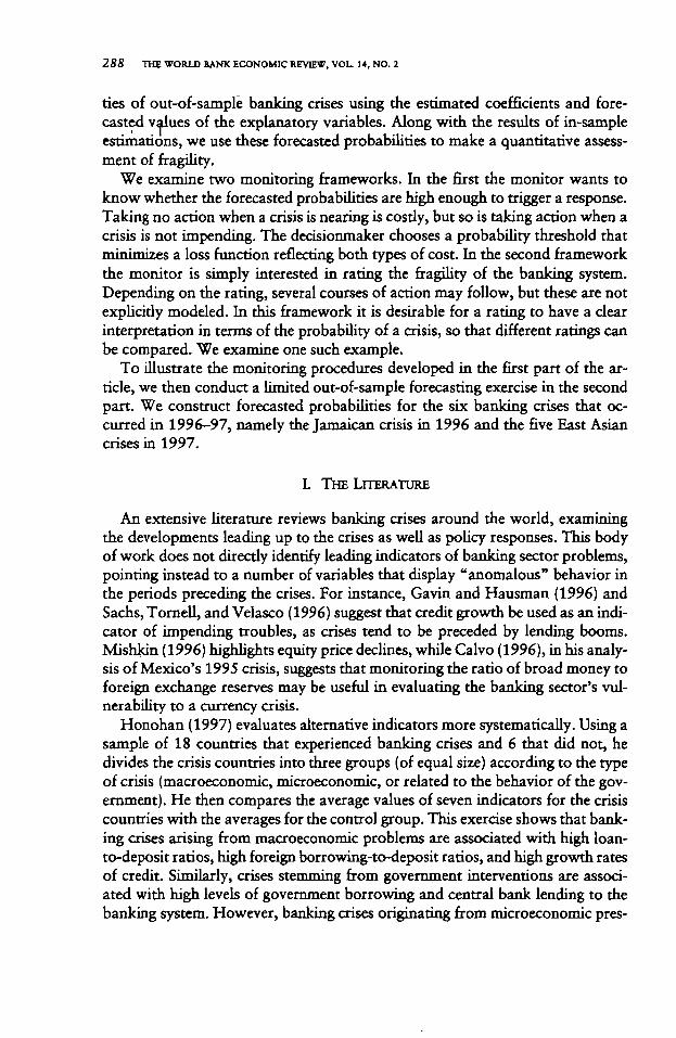
288 THE WORLD BANK ECONOMIC REVIEW, VOL 14, NO. 2

ties of out-of-sample banking crises using the estimated coefficients and fore-casted values of the explanatory variables. Along with the results of in-sampleestimations, we use these forecasted probabilities to make a quantitative assess-ment of fragility.

We examine two monitoring frameworks. In the first the monitor wants toknow whether the forecasted probabilities are high enough to trigger a response.Taking no action when a crisis is nearing is costly, but so is taking action when acrisis is not impending. The derisionmaker chooses a probability threshold thatminimizes a loss function reflecting both types of cost. In the second frameworkthe monitor is simply interested in rating the fragility of the hanking system.Depending on the rating, several courses of action may follow, but these are notexplicitly modeled. In this framework it is desirable for a rating to have a clearinterpretation in terms of the probability of a crisis, so that different ratings canbe compared. We examine one such example.

To illustrate the monitoring procedures developed in the first part of the ar-ticle, we then conduct a limited out-of-sample forecasting exercise in the secondpart. We construct forecasted probabilities for the six banking crises that oc-curred in 1996-97, namely the Jamaican crisis in 1996 and the five East Asiancrises in 1997.

L THE LITERATURE

An extensive literature reviews banking crises around the world, examiningthe developments leading up to the crises as well as policy responses. This bodyof work does not directly identify leading indicators of banking sector problems,pointing instead to a number of variables that display "anomalous" behavior inthe periods preceding the crises. For instance, Gavin and Hausman (1996) andSachs, Tornell, and Velasco (1996) suggest that credit growth be used as an indi-cator of impending troubles, as crises tend to be preceded by lending booms.Mishkin (1996) highlights equity price declines, while Calvo (1996), in his analy-sis of Mexico's 1995 crisis, suggests that monitoring the ratio of broad money toforeign exchange reserves may be useful in evaluating the banking sector's vul-nerability to a currency crisis.

Honohan (1997) evaluates alternative indicators more systematically. Using asample of 18 countries that experienced banking crises and 6 that did not, hedivides the crisis countries into three groups (of equal size) according to the typeof crisis (macroeconomic, microeconomic, or related to the behavior of the gov-ernment). He then compares the average values of seven indicators for the crisiscountries with the averages for the control group. This exercise shows that bank-ing crises arising from macroeconomic problems are associated with high loan-to-deposit ratios, high foreign borrowing-to-deposit ratios, and high growth ratesof credit. Similarly, crises stemming from government interventions are associ-ated with high levels of government borrowing and central bank lending to thebanking system. However, banking crises originating from microeconomic pres-

DemtrgUf-Kuttt and Detragiache 289

sures do not appear to be associated with abnormal behavior on the part of theindicators examined in the study.

Rojas-Suarez |[1998) proposes an approach based on bank-level indicators,similar in spirit to the CAMEL system used by U.S. regulators to identify problembanks. She argues that in emerging markets (particularly those in Latin America)CAMEL indicators are not good signals of bank strength and that more informa-tion can be obtained by monitoring the deposit interest rate, the spread betweenthe lending and deposit rates, the growth rate of credit, and the growth rate ofinterbank debt. Because these variables are measured against banking systemaverages, however, this approach appears more adequate for identifying weak-nesses specific to individual banks than for identifying systemic fragility. Theapproach also requires bank-level information, which often is not readily avail-able in developing countries.

To date, Kaminsky and Reinhart (1999) have made the most comprehensiveeffort to develop a set of early warning indicators for banking crises (and cur-rency crises). The methodology is refined in Kaminsky (1998). These studies ex-amine the behavior of 15 macroeconomic indicators for a sample of 20 countriesthat experienced banking crises during 1970-95.2 The authors compare the be-havior of each indicator in the 24 months prior to the crisis with the behaviorduring tranquil times. A variable is deemed to signal a crisis if it crosses a particu-lar threshold at any time. If that signal is followed by a crisis within the next 24months, then it is considered correct; otherwise it is considered noise. The thresh-old for each variable is chosen to minimi?/* the in-sample noise-to-signal ratio.The authors then compare the performance of different indicators based on theassociated type I and type II errors, the noise-to-signal ratio, and the probabilityof a crisis occurring conditional on a signal being issued.3

The indicator with the lowest noise-to-signal ratio and the highest probabilityof crisis conditional on the signal is the real exchange rate, followed by equityprices and the money multiplier. These three indicators, however, have a highincidence of type I errors, as they fail to issue a signal in 73-79 percent of theobservations in the 24 months preceding a crisis. The incidence of type II errors,in contrast, is much lower, ranging from 8 to 9 percent. The variable with thelowest type I error is the real interest rate, which issues a signal in 30 percent ofthe observations preceding a crisis. The high incidence of type I errors relative totype II errors may not be a desirable feature of a warning system if the costs ofraising a false alarm are small relative to the costs of failing to anticipate a crisis.

Since, presumably, the likelihood of a crisis is greater when several indicatorssignal simultaneously, Kaminsky (1998) develops composite indexes. These in-clude the number of indicators that cross the threshold at any given time or aweighted variant of that index in which each indicator is weighted by its signal-to-noise ratio so that more informative indicators receive more weight. The best

2. For a study of early warning indicators of currency crises, see also IMF (1998).3. The authors use an adjusted version of the noise-to-signal ratio, computed as the ratio of the probability

of a type II error to 1 minus the probability of a type I error.

290 THE •WORLD BANK ECONOMIC REVIEW, VOL 14, NO. 2

composite indicator outperforms the real exchange rate in predicting crises in thesample, but it is worse at predicting observations of no crisis.4

The approach we develop here will allow policymakers to choose a warningsystem that reflects the relative cost of type I and type II errors, and it will offer anatural way of measuring the combined effect of various economic forces onbanking sector vulnerability. By making better use of all available information,the system will produce lower overall in-sample forecasting errors than wouldindividual indicators. We also examine a problem not addressed by Kaminskyand Reinhart (1999), that of a monitor who wishes to use information containedin the statistical analysis of past crises not just to anticipate a crisis but also tomake a more nuanced assessment of banking sector fragility.

n. ESTIMATING THE PROBABILITIES OF IN-SAMPLE BANKING CRISES IN A

MULTTVARIATE L O O T FRAMEWORK

The starting point of our analysis is an econometric model of the probabilityof a systemic banking crisis. In Demirguc,-Kunt and Detragiache (1998,1999) weestimate alternative specifications of a logit regression for a large sample of de-veloping and industrial countries, including countries that experienced bankingcrises and those that did not. Details on sample selection, the construction of thebanking crisis variable, and the choice of explanatory variables can be foundthere.

To form the basis of an easy-to-use monitoring system, we estimate a specifi-cation of our empirical model that includes only variables that are available fromthe IMF's International Financial Statistics or other publicly available databasesand that are routinely forecasted by the IMF in its biannual World EconomicOutlook or by professional forecasters. As it turns out, this is not the specifica-tion that best fits the data. We estimate the regression using a panel of 766 obser-vations for 65 countries during 1980-95.5 In this panel we identify 36 systemicbanking crises, so that crisis observations make up 4.7 percent of the sample(table 1). The set of explanatory variables capturing macroeconorhic conditionsincludes the growth rate of real gross domestic product (GDP), the change in theterms of trade, the rate of depreciation of the exchange rate (relative to the U.S.dollar), the rate of inflation, and the fiscal surplus as a share of GDP. The explana-tory variables capturing characteristics of the financial sector are the ratio ofbroad money to foreign exchange reserves and the growth rate of bank creditlagged two periods. Finally, GDP per capita proxies for structural characteristicsof the economy.

4. Kaminsky (1998) finds that the probability of a crisis computed by taking into account the numberof indicaton irignaling a crisis increased substantially before the 1997 crises in the Philippines, Malaysia,and Thailand, but not in Indonesia. The Republic of Korea was not part of the sample.

5. Because of missing data or breaks in die series, part of the sample period may be excluded for somecountries. Years in which banking crises are ongoing also are excluded from ihe sample.

Demtrg&f-Kimt and Detragiache 291

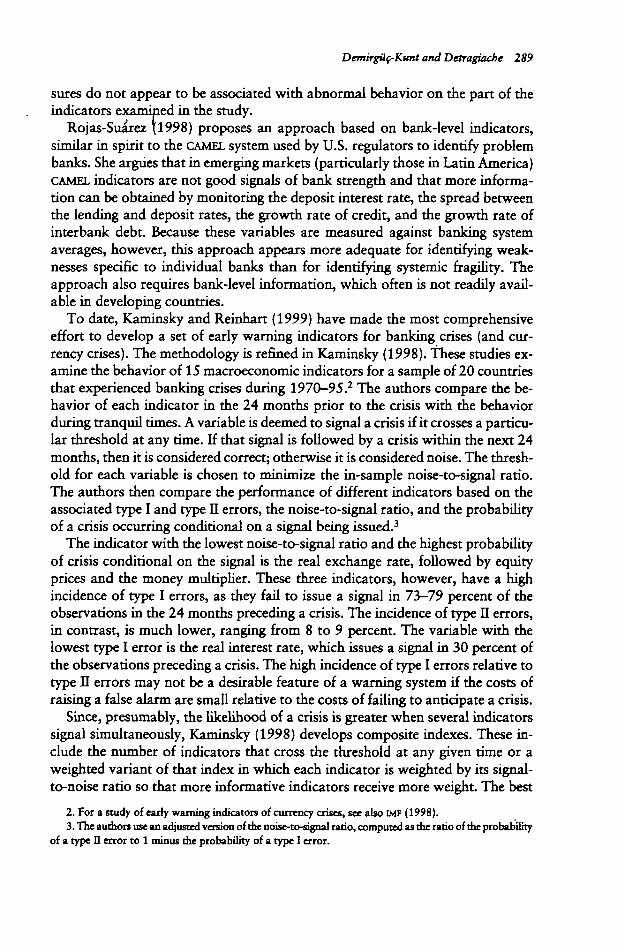
Table 1. Banking Crises and Estimated Probabilities of CrisesCountry

ChileColombiaEcuador£1 SalvadorFinlandGuyanaIndiaIndonesiaIsraelItalyJapanJordanKenyaMalaysiaMaliMexicoMexicoNepalNigeriaNorwayPanamaPapua New GuineaPeruPhilippinesPortugalSouth AfricaSri LankaSwazilandSwedenTanzaniaThailandTurkeyTurkeyUnited StatesUruguayVenezuela

Crisis year

198119821995198919911993199119921983199019921989199319851987198219941988199119871988198919831981198619851989199519901988198319911994198019811993

Estimated probability

0.2310.0660.4390.0550.0660.0070.0690.1070.9990.0150.0370.3340.3610.0670.0350.5270.0990.0180.0110.0360.5390.1210.2440.0350.0640.1960.0360.6330.0360.0350.0270.1580.4820.2380.3290.494

Source: Authors' calculations.

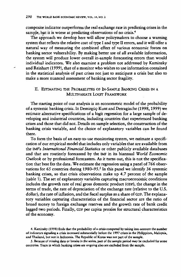
The estimated coefficients of the logit regression reveal that low GDP growth, ahigh real interest rate, high inflation, strong growth of bank credit in the past,and a high ratio of broad money to reserves are all associated with a high prob-ability of a banking crisis (table 2). Exchange rate depreciation, the terms oftrade, the fiscal surplus, and GDP per capita are not significant. The estimatedprobability of a crisis for the 36 episodes included in the sample ranges from alow of 1.1 percent for Nigeria to a high of 99.9 percent for Israel (see table 1).About 70 percent of the episodes have an estimated probability of 4 percentor more, while only 17 percent have an estimated probability of more than50 percent.

2 9 2 THE -WORLD RANK ECONOMIC REVIEW, VOL. 14, NO. 2

Table 2. Logit Regression of the Probability of a Banking CrisisExplanatory variable Estimated coefficient

GDP Growth -0.172*(0.034)

Change in terms of trade -0.021(0.018)

Depreciation 0.007(0.006)

Real interest rate 0.065*(0.016)

Inflation 0.020**(0.010)

Ratio of fiscal surplus to GDP 0.066(0.036)

Ratio of M2 to reserves 0.013*(0.005)

Credit growth,_2 0.015**(0.008)

GDP per capita -0.039(0.033)

Number of crises 36Number of observations 766Model x1 61.46*AIC 249

'Significant at the 1 percent level.* 'Significant at the 5 percent leveLNote: Standard errors are in parentheses,a. Akaike's Information Criterion.Source: Authors' calculations.

Sources of Fragility: The 1994 Mexican Crisis

One of the advantages of the muJtivariate logit model is that we can easilyidentify the sources of fragility by calculating the contribution of each explana-tory variable to a change in the estimated probability of a crisis. As an illustra-tion, we analyze the factors that contributed to the sharp increase in the esti-mated probability of a crisis in Mexico in 1993, just before the actual crisisoccurred in 1994 (table 3).

In 1993 high past credit growth, high real interest rates, and high inflationwere the main factors underlying the high probability of a crisis in Mexico. Be-cause the logit is nonlinear, the sum of the contribution of each variable to thechange in probability does not always add up to the total change (see the lastcolumn of table 3). Looking at macroeconomic factors, we see that Mexico hada negative growth shock that significantly raised the probability of a crisis. Realinterest rates also rose significantly, and there was a minor terms-of-trade shock.At the same time, appreciation of the exchange rate, lower inflation, and a lowerbudget surplus offset some of this increase.

Financial sector variables played a less important role in explaining the overallincrease in probability, slightly offsetting the impact of the macroeconomic fac-

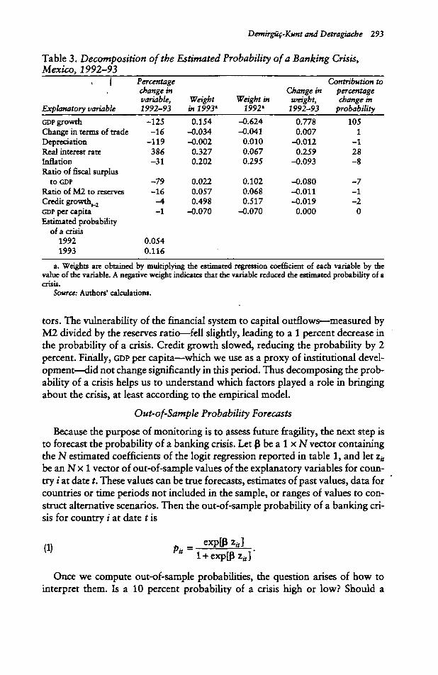
Demirguc-Kunt and Detragiacbe 293

Table 3. Decomposition of the Estimated Probability of a Banking Crisis,Mexico, 1992-93

. 1

Explanatory variable

GDP growthChange in terms of tradeDepreciationReal interest rateInflationRatio of fiscal surplus

t o GDP

Ratio of M2 to reservesCredit growth^GDP per capitaEstimated probability

of a crisis19921993

Percentagechangemvariable,1992-93

-125-16

-119386-31

-79-16

-A-1

0.0540.116

Weightin 1993'

0.154-0.034-0.0020.3270.202

0.0220.0570.498

-0.070

Weight in1992'

-0.624-0.0410.0100.0670.295

0.1020.0680.517

-0.070

Change inweight,

1992-930.7780.007

-0.0120.259

-0.093

-0.080-0.011-0.0190.000

Contribution topercentagechangem

probability

1051

-128-8

-7-1-20

a. Weights are obtained by multiplying the estimated regression coefficient of each variable by thevalue of die variable. A negative weight indicates that die variable reduced die estimated probability of acrisis.

Source: Authors' calculations.

tors. The vulnerability of the financial system to capital outflows—measured byM2 divided by the reserves ratio—fell slightly, leading to a 1 percent decrease inthe probability of a crisis. Credit growth slowed, reducing the probability by 2percent. Finally, GDP per capita—which we use as a proxy of institutional devel-opment—did not change significantly in this period. Thus decomposing the prob-ability of a crisis helps us to understand which factors played a role in bringingabout the crisis, at least according to the empirical model.

Out-of-Sample Probability Forecasts

Because the purpose of monitoring is to assess future fragility, the next step isto forecast the probability of a banking crisis. Let 3 be a 1 x N vector containingthe N estimated coefficients of the logit regression reported in table 1, and let Zj,be an N x 1 vector of out-of-sample values of the explanatory variables for coun-try i at date t. These values can be true forecasts, estimates of past values, data forcountries or time periods not included in the sample, or ranges of values to con-struct alternative scenarios. Then the out-of-sample probability of a banking cri-sis for country i at date t is

_ expfl zft](1)

Once we compute out-of-sample probabilities, the question arises of how tointerpret them. Is a 10 percent probability of a crisis high or low? Should a

294 THE WORLD BANK ECONOMIC REVffiW, VOL. 14, NO. 2

policymaker take preventive actions when faced with such a probability? Should asurveillance agency issue a warning? In the next section we address such questions.

in. BUILDING AN EARLY WARNING SYSTEM USLNG

ESTIMATED CRISIS PROBABILITIES

The first monitoring framework that we consider is one in which thedecisionmaker must decide whether the forecasted probability is large enough toissue a warning. This is the framework implicit in Kaminsky and Reinhart (1999).Issuing a warning will lead to some sort of preventive action. For instance, thedecisionmaker may invest in gathering further information, such as acquiringbank-level balance sheet data or holding discussions with senior bank managers,bank supervisory agencies, or other market participants. Alternatively, thedecisionmaker may use the monitoring system to decide whether to take preven-tive policy measures, such as tightening prudential capital or Liquidity require-ments for banks or reducing interest rates to ease pressures on bank balancesheets. For a warning system to be useful, preventive measures must substantiallyreduce the costs of a crisis. "We assume that this is the case. Also a useful warningsystem should minimize false alarms, since preventive measures are usually costly.Tighter prudential requirements may cause banks to cut credit, perhaps leadingto a credit crunch; looser monetary policy may lead to higher inflation.

The choice of the threshold for issuing a warning will generally depend onthree factors. The first is the probability of type I and type II errors associatedwith the threshold, which, assuming that the sample of past crises is representa-tive of future crises, can be assessed on the basis of the in-sample frequency of thetwo errors. Clearly, the higher is the threshold that forecasted probabilities mustcross before a warning is issued, the higher will be the probability of a type Ierror and the lower will be the probability of a type II error (and vice versa).

The second parameter on which the choice of the threshold depends is theunconditional probability of a banking crisis, which can also be assessed basedon the in-sample frequency of crisis observations. If crises tend to be rare events,then the overall Likelihood of making a type I error is relatively small (and viceversa). Finally, the third factor is the cost to the decisionmaker of taking preven-tive actions relative to the cost of failing to anticipate a banking crisis. In generaL,these costs to the decisionmaker are themselves forecasts of the true costs, andmaking a good decision requires having good forecasts. A policymaker who tendsto underestimate the cost of a crisis or to overestimate the cost of taking preven-tive actions will be too conservative in choosing a warning threshold (and viceversa).6

A Loss Function for the Decisionmaker

Based on these considerations, we can develop a more formal analysis of thedecision process behind the choice of a warning system. Let T be the threshold

6. For estimates of the fiscal costs of recent banking crises, see Caprio and Klingebiel (1996).

Demtrgtif-Ktmt and Detragiache 295

chosen by the decisionmaker, so that if the forecasted probability of a crisis forcountry i at time t exceeds T, the system will issue a warning. Let p(T) denote theprobability that the system will issue a warning, and let e(T) be the joint prob-ability that a crisis will occur and the system will not issue a warning. Further, letCi be the cost of taking preventive actions as a result of having received a warn-ing, and let c2 be the additional cost of a banking crisis if it is not anticipated (ifanticipating a crisis can prevent it altogether, then c2 is the entire cost of thecrisis). Presumably, C\ is substantially smaller than Cj if further information gath-ering will be useful and if the knowledge that a crisis is impending will allowpolicymakers to take effective preventive measures. Then we can define a simplelinear expected loss function for the decisionmaker as

(2) L(T)mp(T)c1+ e(7>2-

Let a(l) be the type I error associated with threshold T (the probability of notreceiving any warning conditional on a crisis occurring), and let b(T) be the prob-ability of a type II error (the probability of receiving a .warning conditional on nocrisis taking place). Also let w denote the (unconditional) probability of a crisis.Then we can rewrite the loss function of the decisionmaker as

(3) L(T) = cj(l - a(T))w

The second part of the equality shows that the higher is the cost of missing acrisis relative to the cost of taking preventive action (the larger is c2 relative to Cj),the more concerned will the decisionmaker be about a type I error relative to atype II error (and vice versa). Also the higher is the unconditional probability ofa banking crisis (measured by the parameter w), the more weight will thedecisionmaker place on type II errors, as the frequency of false alarms is greaterwhen crises tend to be rare events.7

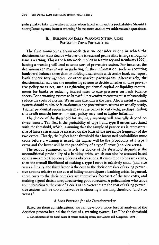
Using in-sample frequencies as estimates of the true parameters, w should equalthe frequency of banking crises in the sample, namely 0.047 (see table 1). We canobtain the functions a(T) and b{T), which trace how error probabilities changewith the threshold for issuing warnings, from the in-sample estimations as fol-lows. Given a threshold of, say, T = 0.05, we can derive a(0.05), that is, theassociated probability of a type I error, as the percentage of banking crises in thesample with an estimated probability below 0.05. Similarly, 6(0.05), the prob-ability of issuing a warning when no crisis occurs, is the percentage of observa-tions in which no crisis occurs when the estimated probability of a crisis is above0.05. For T € [0, 1], a(T) is increasing, since the probability of not issuing a

7. A risk-averse decisionaiaker would place greater weight on minimizing type I errors than on minimizingtype II errors, since type I errors are more costly. We are indebted to a referee for suggesting this point.

2 9 6 THE WORLD BANK ECONOMIC REVIEW, VOL. 14, NO. 2

Figure 1. Crisis Threshold and In-Sample Classification Accuracy

, Probability of error

0.1 0.2 0.3 0.4 0.5 0.6

Probability threshold

0.7 0.8 0.9 1

Source: Authors' calculations.

warning when a crisis occurs increases as the threshold rises, while b(T) is de-creasing (figure 1). The two functions cross at T = 0.036, at which the probabil-ity of either type of error is about 30 percent.

Figure 1 also shows that probabilities estimated through our multivariate logitframework can provide a more accurate basis for an early warning system thanthe indicators developed by Kaminsky and Reinhart (1999). The indicator asso-ciated with the lowest type I error in the Kaminsky-Reinhart framework is thereal interest rate, with a type I error of 70 percent and a type LI error of 19percent. In our model a threshold for a type I error of 72 percent comes at thecost of a type II error of only 1.2 percent. Similarly, the best indicator of bankingcrises according to Kaminsky and Reinhart is the real exchange rate, with a typeI error of 73 percent and a type LI error of 8 percent (resulting in an adjustednoise-to-signal ratio of 0.30). With our model we can obtain a type LI error of 7.4percent by choosing a probability threshold of 0.09, which is associated with atype I error of only 53 percent. The adjusted noise-to-signal ratio is 0.25. Thebetter performance of the multivariate logit model Likely stems from the fact thatit combines into one number (the estimated probability of a crisis) all of theinformation provided by the economic variables monitored.8

8. The logit parameters are estimated using maximum likelihood, and the likelihood function does nottake into account the different costs of type I and type II errors. One way to improve the warning systemcould be to choose parameters that minimi^ the dedsionmaker's loss functions.

Demirguf-Kunt and Detragiache 297

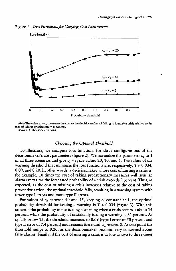
Figure 2. Loss Functions for Varying Cost Parameters

Loss1 function

0.1 0.2 0.3 0.4 0.5 0.6 0.7

Probability threshold

0.8 0.9

Note: The value c, - c, measures the cost to the dedsionmaker of failing to identify a crisis relative to thecost of taking precautionary measures.

Source: Authors' calculations.

Choosing the Optimal Threshold

To illustrate, we compute loss functions for three configurations of thedecisionmaker's cost parameters (figure 2). We normalize the parameter cx to 1in all three scenarios and give c2 - C\ the values 20, 10, and 5. The values of thewarning threshold that minimi7.fi the loss functions are, respectively, T = 0.034,0.09, and 0.20. In other words, a decisionmaker whose cost of missing a crisis is,for example, 10 times the cost of taking precautionary measures will issutanalarm every time the forecasted probability of a crisis exceeds 9 percent. Thus, asexpected, as the cost of missing a crisis increases relative to the cost of takingpreventive action, the optimal threshold falls, resulting in a warning system withfewer type I errors and more type II errors.

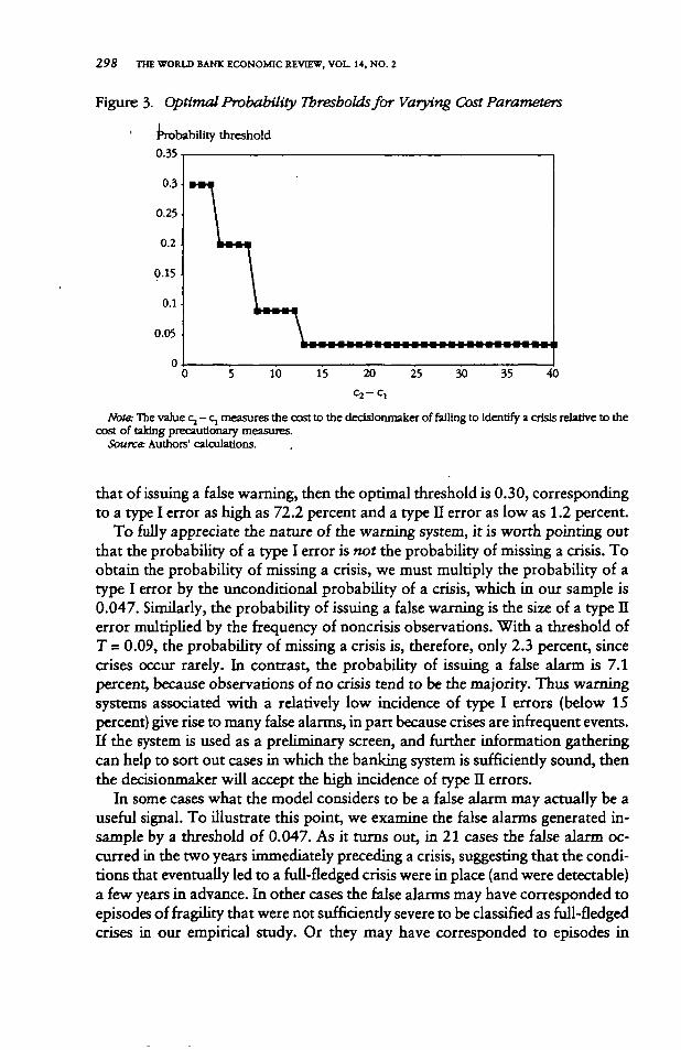
For values of c2 between 40 and 15, keeping cx constant at 1, the optimalprobability threshold for issuing a warning is T = 0.034 (figure 3). With thiscriterion the probability of not issuing a warning when a crisis occurs is about 14percent, while the probability of mistakenly issuing a warning is 31 percent. Asc2 falls below 15, the threshold increases to 0.09 (type I error of 50 percent andtype II error of 7.4 percent) and remains there until c2 reaches 8. At that point thethreshold jumps to 0.20, as the decisionmaker becomes very concerned aboutfalse alarms. Finally, if the cost of missing a crisis is as low as two to three times

298 THE WORLD BANK ECONOMIC REVIEW, VOL. 14, NO. 2

Figure 3. Optimal Probability Thresholds for Varying Cost Parameters

Probability threshold

Not& The value Cj - c, measures the cost to the dedstonmaker of falling to Identify a crisis relative to thecost of taking precautionary measures.

Source: Authors' calculations.

that of issuing a false warning, then the optimal threshold is 0.30, correspondingto a type I error as high as 72.2 percent and a type LT error as low as 1.2 percent.

To fully appreciate the nature of the warning system, it is worth pointing outthat the probability of a type I error is not the probability of missing a crisis. Toobtain the probability of missing a crisis, we must multiply the probability of atype I error by the unconditional probability of a crisis, which in our sample is0.047. Similarly, the probability of issuing a false warning is the size of a type IIerror multiplied by the frequency of noncrisis observations. With a threshold ofT = 0.09, the probability of missing a crisis is, therefore, only 2.3 percent, sincecrises occur rarely. In contrast, the probability of issuing a false alarm is 7.1percent, because observations of no crisis tend to be the majority. Thus warningsystems associated with a relatively low incidence of type I errors (below 15percent) give rise to many false alarms, in part because crises are infrequent events.If the system is used as a preliminary screen, and further information gatheringcan help to sort out cases in which the banking system is sufficiently sound, thenthe decisionmaker will accept the high incidence of type LI errors.

In some cases what the model considers to be a false alarm may actually be auseful signal. To illustrate this point, we examine the false alarms generated in-sample by a threshold of 0.047. As it turns out, in 21 cases the false alarm oc-curred in the two years immediately preceding a crisis, suggesting that the condi-tions that eventually led to a full-fledged crisis were in place (and were detectable)a few years in advance. In other cases the false alarms may have corresponded toepisodes of fragility that were not sufficiently severe to be classified as full-fledgedcrises in our empirical study. Or they may have corresponded to episodes in

DemtrgQf-Kunt and Detragiache 299

which a crisis was prevented by a prompt policy response. Thus assessing theaccuracy of the warning system based on the accuracy of in-sample classificationmay exaggerate the incidence of type II errors. However, out-of-sample predic-tions are subject to additional sources of error relative to in-sample predictions:the forecasted values of the explanatory variables include forecast errors, andthere may be structural breaks in the relationship between banking sector fragil-ity and the explanatory variables, making predictions based on past behaviorinadequate. Also, despite the large size of our panel, the number of systemicbanking crises (36) is still relatively small, so that small-sample problems mayaffect the estimation results. As more data become available and the size of thepanel is extended, this problem should become less severe.

Comparing the Loss Function with the Noise-to-Signal Ratio

It is of interest to compare the optimal threshold derived from minimising theloss function proposed here with the optimal threshold that would result fromminimizing the (adjusted) noise-to-signal ratio, the criterion used by Kaminskyand Reinhart (1999). Define the noise-to-signal ratio as

(4)\-b(T)

Then the loss function can be rewritten as

(5) L(T) = wci +w(c2 -Cj)a(T) + (1

and the first-order condition for the minimization of the loss function is

(6) ^ - E [wfa - cj) - (1 - w)c,NS{T)y(T) + (1 - w)cj\ - a(T)]N'S(T) = 0.al

Suppose T" is the threshold that minimizes the noise-to-signal ratio. Then, at T =T", NS'(T) = 0, and the derivative of the loss function is

(7)

For a convex loss function a positive (negative) sign for equation 7 means thatthe threshold T" is too large (small) relative to the threshold that would mini-mize the loss function. Accordingly, if equation 7 is positive (negative), by mini-mizing the noise-to-signal ratio, the decisionmaker.will make too many type I(type II) errors relative to the threshold that minimizes the loss function. Sincerf'(T) > 0 (the probability of a type I error is increasing in the threshold), equation7 has the sign of the term in square brackets. This term is more likely to bepositive the larger is the cost of a type I error (c2 - ct) relative to the cost of a typeII error (cj) and the larger is the unconditional probability of a crisis. Thus ifbanking crises tend to be rare, and the cost of missing a crisis is high relative to

300 THE WORLD BANK ECONOMIC REVIEW, VOL. 14, NO. 2

the cost of raising a false alarm, minimizing the noise-to-signal ratio is likely toyield a choice criterion that results in too many missed crises for a decisionmakerwhose preferences are captured by the linear loss function of equation 5.

IV. CONSTRUCTING A SYSTEM FOR RATING BANK FRAGILITY

In this section we consider the problem of a monitor who must rate the fragil-ity of a given banking system. Other agents will then use the rating to decide ona possible policy response, but the monitor is not necessarily aware of the costsand benefits of such policy actions. Another rationale for using fragility classesinstead of a critical threshold as a monitoring device is that small changes in thecritical threshold may lead to substantial differences in type I and type II errors,as seen in figure 1. In constructing fragility classes, the classification criterionshould have a clear interpretation in terms of type I and type II errors. This hastwo advantages: first, agents who learn the rating can make their own cost-benefit calculations when they decide whether or not to take action, and, second,the fragility of two systems that are assigned different ratings can be comparedbased on a clear metric.

The starting point is once again the set of forecasted crisis probabilities ob-tained using the coefficients estimated in the multivariate logit regression. Clearly,a country with a forecasted probability of x should be deemed more fragile thanone with an estimated probability of y < x. To establish fragility classes, we canpartition the interval [0, 1], which is the set of possible forecasted probabilities,into a number of subintervals and assign a rating to all estimated probabilitieswithin a given class.

There are no objective criteria for choosing one partition over another, but anumber of considerations help to narrow the choices. First, because the frequencyof crises in the sample is low, choosing a fine partition would give misleadingresults, because many classes would have no observed crises. For instance, in oursample there are no episodes with an estimated crisis probability between 4 and5 percent, whereas there are episodes with an estimated probability between 3and 4 percent (see figure 1). If we choose the intervals [0.04-0.05] and [0.03-0.04] as two of the classes, then it would appear that fragility decreases with theestimated probability of a crisis—an obviously misleading conclusion.

Another caveat is that the empirical distribution of the estimated probabilitiesis strongly skewed toward zero: only 8.5 percent of the observations have prob-abilities higher than 10 percent, and more than 45 percent are in the 0-2 percentrange. Thus partitioning the unit interval by subsets of the same size'would as-sign an uneven number of observations to each class, with very few observationsin the highest probability intervals.

Based on these considerations, we construct a rating system with four fragilityclasses (table 4). We choose the upper bounds of each of the four classes so thatthe type I error associated with the bounds are 10, 30, 50, and 100 percent,respectively. According to this criterion, observations with forecasted probabili-

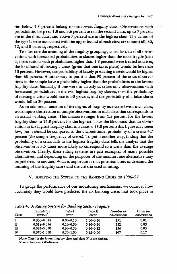
Demirguf-Kunt and Detragiache 301

ties below 1.8 percent belong to the lowest fragility class. Observations withprobabilities, between 1.8 and 3.6 percent are in the second class, up to 7 percentare in the third class, and above 7 percent are in the highest class. The values ofthe type II error associated with the upper bound of each class are (about) 60,30,12, and 0 percent, respectively.

To illustrate the meaning of the fragility groupings, consider that if all obser-vations with forecasted probabilities in classes higher than the most fragile (thatis, observations with probabilities higher than 1.8 percent) were treated as crises,the likelihood of missing a crisis (given that one takes place) would be less than10 percent. However, the probability of falsely predicting a crisis would be higherthan 60 percent. Another way to put it is that 90 percent of the crisis observa-tions in the sample have a probability higher than the probabilities in the lowestfragility class. Similarly, if one were to classify as crises only observations withforecasted probabilities in the two highest fragility classes, then the probabilityof missing a crisis would rise to 30 percent, and the probability of a false alarmwould fall to 30 percent.

As an additional measure of the degree of fragility associated with each class,we compute the fraction of sample observations in each class that corresponds toan actual banking crisis. This measure ranges from 1.5 percent for the lowestfragility class to 16.8 percent for the highest. Thus the likelihood that an obser-vation in the highest fragility class is a crisis is 16.8 percent; this figure may seemlow, but it should be compared to the unconditional probability of a crisis: 4.7percent (the sample frequency of crises). To put it another way, finding that theprobability of a crisis falls in the highest fragility class tells the analyst that theobservation is 3.5 times more likely to correspond to a crisis than the averageobservation. Clearly, these rating systems are just examples of many possiblealternatives, and depending on the purposes of the monitor, one alternative maybe preferred to another. What is important is that potential users understand themeaning of the fragility score and the criteria used in rating.

V. APPLYING THE SYSTEM TO THE BANKING CRISES OF 1996-97

To gauge the performance of our monitoring mechanisms, we consider howaccurately they would have predicted the six banking crises that took place in

Table 4. A Rating System for Banking Sector Fragility

Class

I

nmIV

Probabilityinterval

0.000-0.0180.018-O.0360.036-0.0700.070-1.000

Type Ierror

0.00-0.100.10-0300.30-0.500.50-1.00

Type IIerror

1.00-0.600.60-0.300.30-0.120.12-0.00

Number ofobservations

291232136107

Crisis perobservation

0.010.030.050.17

Note: Class I is the lowest fragility class and class IV is the highest.Source: Authors' calculations.

3 02 THE WORLD BANK ECONOMIC REVIEW, VOL 14, NO. 2

1996-97, that is, after the end of the sample period used in the estimation exer-cise abovef The banking crises occurred in Jamaica in 1996 and in Indonesia, theRepublic of Korea, Malaysia, the Philippines, and Thailand in 1997. Early ac-counts and analyses of the events surrounding the five Asian crises can be found,for instance, in IMF (1997), Radelet and Sachs (1998), and Goldstein and Hawkins(1998).

To compute the probabilities of out-of-sample banking crises for the six coun-tries, we use two sets of values for the explanatory variables. The first set consistsof actual realizations. The out-of-sample probabilities obtained in this way arenot true forecasts, of course. In particular, for the five Asian countries these fig-ures capture the large exchange rate depreciations that took place in the secondhalf of 1997 and their immediate consequences. It is of interest to try to assesswhether signs of increasing banking sector fragility would have been apparentbefore the depreciations took place, since they were largely unanticipated by ob-servers. To this end, and, more generally, to assess the performance of the moni-toring system when true forecasts are used, we also compute out-of-sample prob-abilities using forecasts of the explanatory variables as of April-May 1997.Comparing the two forecasts will reveal the extent to which errors in forecastingthe explanatory variables would have clouded the fragility assessment based onour model.

We take the forecasted values of the explanatory variables, where available,from the Financial Times' Currency Forecaster, and from Consensus Forecasts.These works survey several prominent private sector forecasters and publish themeans of their forecasts. For the five Asian countries the growth rate of real GDP,inflation, exchange rate depreciation, and the real interest rate are from the Cur-rency Forecaster, and broad money is from Consensus Forecasts. The remainingvalues (and all of the values for Jamaica) are from the May 1997 round of theIMF's"semiannual World Economic Outlook.9 To compute the probabilities ofout-of-sample crises using realized values of the explanatory variables, we usenumbers from the International Financial Statistics when available and February1998 numbers from the World Economic Outlook otherwise.

Based on forecasts as of April-May 1997, the estimated probabilities of criseswere relatively low for the five Asian countries, whereas Jamaica was well intothe highest fragility zone as early as 1995 (figure 4). This is not surprising, sinceall the Asian countries had very good macroeconomic performances in the yearsup to 1996—performances that, by and large, were expected to continue. InJamaica the forecasted probability of a crisis was 14 percent in 1995 and 13percent in 1996. The two main factors contributing to the increase in the prob-ability of a crisis were high real interest rates and high inflation. Strong past

9. There are two exception*. For the Philippine*, broad money come* from the Worid Economic Outlook.For Korea, no forecast of reserves was available, so we arbitrarily assumed that reserves returned to their1995 value in 1997.

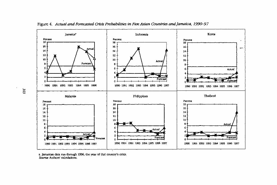
Figure 4. Actual and Forecasted Crisis Probabilities in Five Asian Countries and Jamaica, 1990-97

S

Jamaica"Percent

1990 1991 1992 1993 1994 1995 1996

Indonesia

Percent

1990 1991 1992 1993 1994 1995 1996 1997

Korea

Percent

16-

14

12-

10-

8-

6-

2-

0-

-JC—.W1 T—i 1—-?̂

Actual

JB'^Forecaa

1990 1991 1992 1993 1994 1995 1996 1997

Malaysia Philippines Thailand

Percent Percent Percent

16-14

12

10

864

n

w

1 1 1 —>

/

/Actual /

/

—i T™

1990 1991 1992 1993 1994 1995 1996 1997 1990 1991 1992 1993 1994 1995 1996 1997 1990 1991 1992 1993 1994 1995 1996 1997

a. Jamaican data run through 1996, the year of that country's crisis.Sourca Authors' calculations.

3 04 THE WORLD BANK ECONOMIC REVIEW, VOL. 14, NO. 2

credit growth and a favorable fiscal position also contributed to fragility in 1995,but not in |1996.

The two most fragile Asian countries were Thailand and the Philippines, bothhaving a forecasted crisis probability of about 3.5 percent in 1997. This prob-ability would have placed the two countries on the border between the secondand third fragility zones based on our rating system. In Thailand the main factorcontributing to bank fragility both in 1996 and in 1997 was the high real interestrate; strong past credit growth was also a factor. But in contrast with Jamaica,where GDP growth was lackluster, Thailand had a large predicted GDP growthrate, which worked as an offsetting factor, keeping the overall probability of acrisis relatively low. In the Philippines the predicted probability increased morethan 20 percent between 1996 and 1997, mainly because of the high growth rateof credit two years earlier. The real interest rate was lower than that in Thailand,but so was GDP growth.

Indonesia, Malaysia, and Korea all had forecasted crisis probabilities below 3percent in 1996 and in 1997, and would have been placed in the second fragilityclass (actually, Malaysia would have received the lowest fragility rating in 1996).As in Thailand and the Philippines the expectation that the exchange rate wouldremain stable and, especially, that GDP growth would continue to be strong morethan offset the prospect of fragility coming from high real interest rates (except inKorea) and strong past credit expansion. Indonesia's high rate of inflation alsotended to increase bank fragility.

Not surprisingly, the picture obtained by estimating the probabilities of crisesusing the latest available data would have been quite different for the five Asiancountries, but not for Jamaica. The estimated probabilities of crises are in thehighest fragility class for Indonesia and Thailand and in the second highest forthe other three Asian countries. Malaysia, with a probability of 3.7 percent, ap-pears to have been the least fragile.10

Decomposing the probability tells some interesting stories. Of course, the ex-change rate depreciation directly affected fragility in all five countries. However,in 1997 inflation was not much higher than forecasted, so it was not among themain factors contributing to greater banking system vulnerability. In all five coun-tries except Korea lower-than-forecasted GDP growth was one of the main con-tributing factors, as was the higher-than-expected real interest rate (except inThailand).

To summarize, an analysis of banking system fragility using the methods de-veloped in this article would have clearly indicated an impending banking crisisin Jamaica. But although signs of fragility were present in Thailand and the Phil-ippines, the overall image of the five Asian economies would have been fairlyreassuring, as expectations of continued strong economic growth and stable ex-change rates would have offset the negative impact of relatively high real interestrates and strong past credit expansion.

10. Of the five Asian countries, Malaysia is the only one without an IMF program.

DermrgOc-Kunt and Detragiache 305

VL CONCLUSIONS

Econometric analysis of systemic banking crises is a relatively new field ofstudy, and the development and evaluation of monitoring and forecasting toolsbased on the results of such analyses are at an embryonic stage at best. Thepurpose of this article has been not so much to propose one or more "ready-to-use" procedures for decisionmakers, but rather to highlight which elements mustbe evaluated in developing such procedures and to explore some possible av-enues. Specifically, we have developed two monitoring tools using forecastedprobabilities obtained from a multivariate logit model of banking crises. The firstis an early-warning system that issues a signal when the probability of a fore-casted crisis exceeds a certain threshold. The appropriate threshold for issuing awarning can be chosen based on the costs of missing a crisis and the benefits ofavoiding a false alarm. The second monitoring tool is a system for rating bankfragility. Both monitoring tools can be used to economize on precautionary costsby pointing to cases of high fragility that warrant more in-depth monitoring.

Evaluating banking sector fragility along these lines is subject to several poten-tial errors common to all exercises based on forecasts. First, the regression coef-ficients used to compute the forecasted probability of a crisis are only estimatesof the true parameters. Second, new crises may be of a different nature than thoseexperienced in the past, so that the coefficients derived from in-sample esti-mation may be of limited use out-of-sample. This problem may be particularlysevere since banking crises tend to be rare events, and, even though the panelused for in-sample estimation is large (766 observations), crisis episodes onlynumber 36.

Third, forecasts of the explanatory variables are likely to incorporate errors,as vividly illustrated by the example of the five recent Asian crises. Large forecasterrors, in turn, may severely distort the assessment of fragility.11 One way toreduce the impact of forecast errors is to develop alternative scenarios for theexplanatory variables and to examine banking sector fragility in the context ofsuch scenarios. This would be particularly useful, because in many cases bankingcrises are triggered by extreme behavior in one or more explanatory variables (acurrency collapse, a bout of inflation, a drastic deterioration in the terms of trade)in a context in which other elements also contribute to overall fragility. Routineforecasts of economic variables rarely capture extreme events of this sort, whichinstead tend to be discussed as "risk elements" of the overall picture.12 The frame-

11. One direction in which this work can be extended is to explore alternative model specifications andcompare them from the point of view of their usefulness for forecasting (see, for instance, Diebold 1997).Here we have used a specification developed in our previous work after eliminating explanatory variablesfor which forecasts were not readily available. It could be that an even more parsimonious specification ismore suitable for forecasting purposes. We leave this issue to future extensions.

12. This is certainly true of IMF forecasts, which often tend to be excessively optimistic (Mussa andSavastano 1999). For the Asian countries we computed crisis probabilities using the most pessimisticforecasts from the Consensus Forecasts group, but this did not lead to a substantial increase in forecastedcrisis probabilities.

306 THE WORLD BANK ECONOMIC REVIEW, VOL. 14, NO. 2

work developed here would lend itself easily to the evaluation of fragility in alter-native scenarios, since it allows us to isolate the contribution of each explanatoryvariable to the forecasted crisis probability.

Another important caveat is that, although aggregate variables can conveyinformation about the general economic conditions that tend to be associatedwith banking sector fragility, they are silent about the situation of individualbanks or specific segments of the banking sector. So they would not detect crisesthat may develop from specific weaknesses in some market segments and spreadthrough contagion. Also informed observers who are familiar with a particularcountry are likely to be in a better position to detect signs of incoming trouble, sothe information generated by a quantitative approach such as ours should comple-ment, not replace, other sources of information.

A final message from this exercise is that, to be useful, a monitoring systemmust be designed to fit the preferences of the decisionmaker. Thus the develop-ment of a system must be the outcome of an interactive process that involvesboth econometricians and policymakers.

REFERENCES

The word "processed" describes informally reproduced works that may not be com-monly available through library systems.

Calvo, Guillermo A. 1996. "Capital Flows and Macroeconomic Management: TequilaLessons." International Journal of Finance and Economics 1(3)^07-24.

Caprio, Gerard, and Daniela Klingebiel. 1996. "Dealing with Bank Insolvencies: Cross-Country Experience." World Bank Policy Research Working Paper 1620. Washing-ton, D.C.: World Bank.

Consensus Economics. Various years. Consensus Forecasts. London.Demirguc-Kunt, Ash, and Enrica Detragiache. 1998. "The Determinants of Banking Cri-

ses in Developing and Developed Countries." IMF Staff Papers 45(l):81-109.. 1999. "Financial Liberalization and Financial Fragility." In Boris Pleskovic and

Joseph E. Stiglitz, eds., Annual World Bank Conference on Development Economics1998. Washington, D.C.: World Bank.

Diebold, Francis. 1997. Elements of Forecasting. Cincinnati: South-Western College Pub-lishing.

Eichengreen, Barry, and Andrew K. Rose. 1998. "Staying Afloat While the Wind Shifts:External Factors and Emerging-Market Banking Crises." NBER Working Paper 6370.National Bureau of Economic Research, Cambridge, Mass. Processed.

Financial Tunes. Various years. Currency Forecaster. Alexandria, Virginia.Gavin, Michael, and Ricardo Hausman. 1996. "The Roots of Banking Crises: The Macro-

economic Context." In Ricardo Hausman and liliana Rojas-Suarez, eds., Volatile Capi-tal Flows: Taming Their Impact on Latin America. Washington, D.C.: Inter-AmericanDevelopment Bank.

Goldstein, Morris, and John Hawkins. 1998. "The Origins of the Asian Financial Tur-moil." Reserve Bank of Australia, Sydney. Processed.

Demtrgiif-Kunt and Detragiacbe 307

Hardy, Daniel, and Ceyla Pazarbasioglu. 1998. "Leading Indicators of Banking Crises:Was Asia Different?" IMF Working Paper 91. International Monetary Fund, Washing-ton, D.C. Processed.

Honohan, Patrick. 1997. "Banking System Failures in Developing and Transition Coun-tries: Diagnosis and Prediction." BIS Working Paper 39. Bank for International Settle-ments, Basel. Processed.

IMF (International Monetary Fund). 1997. "World Economic Outlook. Interim Assess-ment." Washington, D.C. Processed.

. 1998. World Economic Outlook. Washington, D.C.Kaminsky, Graciela L. 1998. "Currency and Banking Crises: The Early Warnings of Dis-

tress." International Finance Discussion Paper 629. Board of Governors of the FederalReserve System, Washington, D.C.

Kaminsky, Graciela, and Carmen M. Reinhart. 1999. "The Twin Crises: The Causes ofBanking and Balance of Payments Problems." American Economic Review 89(3):473-500.

Lindgren, Carl J., Gillian Garcia, and Michael Saal. 1996. Bank Soundness and Macro-economic Policy. Washington, D.C: International Monetary Fund.

Mishkin, Frederic S. 1996. "Understanding Financial Crises: A Developing Country Per-spective." NBER Working Paper 5600. National Bureau of Economic Research, Cam-bridge, Mass.

Mussa, Michael, and Miguel Savastano. 1999. "The IMF Approach to Stabilization." SBERMacroeconomic Annual 14. Cambridge, Mass.: MIT Press.

Radelet, Steven, and Jeffrey Sachs. 1998. "The Onset of the Asian Financial Crises." InPaul Krugman, ed., Currency Crises. Chicago: University of Chicago Press.

Rojas-Suarez, Lniana. 1998. "Early Warning Indicators of Banking Crises: What Worksfor Developing Countries?" Research Department, Inter-American Development Bank,Washington, D.C. Processed.

Sachs, Jeffrey, Aaron Tornell, and Andres Velasco. 1996. "Financial Crises in EmergingMarkets: The Lessons from 1995." Brookmgs Papers on Economic Activity 1(1996):147-98.