Monitoring of visually graded structural lumber

United StatesDepartment ofAgriculture

Forest Service

ForestProductsLaboratory

ResearchPaperFPL�RP�576

Monitoring ofVisually GradedStructural LumberDavid E. KretschmannJames W. EvansLinda Brown

AbstractTo satisfy the increased demand for forest products, much ofthe future timber supply is expected to be derived from im-proved trees grown on managed plantations. This fast-grownresource will tend to be harvested in short-age rotations andwill contain higher proportions of juvenile wood comparedwith wood in current harvests. As a result, current allowableproperties may need to be reduced in the future. This reportexplores four options for monitoring the properties of fast-grown wood and briefly discusses the advantages and disad-vantages of these approaches. The recommended multiple-stage sampling approach is illustrated in detail using simu-lated results based on the North American In-Grade testresults for Southern Pine. Finally, the report presents detailsof a “real world” example of monitoring lumber propertiescurrently being conducted by the Southern Pine InspectionBureau.

Keywords: monitoring, visually graded structural lumber,Southern Pine

July 1999

Kretschmann, David E.; Evans, James W.; Brown, Linda. 1999. Monitoringof visually graded structural lumber. Res. Pap. FPL–RP–576. Madison, WI:U.S. Department of Agriculture, Forest Service, Forest Products Laboratory.18 p.

A limited number of free copies of this publication are available to thepublic from the Forest Products Laboratory, One Gifford Pinchot Drive,Madison, WI 53705–2398. Laboratory publications are sent to hundredsof libraries in the United States and elsewhere.

The Forest Products Laboratory is maintained in cooperation with theUniversity of Wisconsin.

The use of trade or firm names is for information only and does not implyendorsement by the U.S. Department of Agriculture of any product orservice.

The United States Department of Agriculture (USDA) prohibits discrimina-tion in all its programs and activities on the basis of race, color, nationalorigin, gender, religion, age, disability, political beliefs, sexual orientation,or marital or familial status. (Not all prohibited bases apply to all pro-grams.) Persons with disabilities who require alternative means for commu-nication of program information (braille, large print, audiotape, etc.) shouldcontact the USDA’s TARGET Center at (202) 720–2600 (voice and TDD).To file a complaint of discrimination, write USDA, Director, Office of CivilRights, Room 326-W, Whitten Building, 14th and Independence Avenue,SW, Washington, DC 20250–9410, or call (202) 720–5964 (voice andTDD). USDA is an equal employment opportunity employer.

Research HighlightsPrevious research has helped draw attention to a potentialproblem associated with fast-grown plantation material: thehigher percentage of juvenile wood. The lower mechanicalproperties of juvenile wood, compared with mature wood,account for the inferior properties of aggressively grownplantation wood harvested on short rotations compared withthe properties of longer rotation, naturally suppressed timber.Independent grading agencies have a strong interest in de-termining whether a significant change (particularly a de-crease in material properties) in the lumber resource hasoccurred. The work reported here explores four options formonitoring lumber properties and briefly discusses the ad-vantages and disadvantages of these options. The recom-mended multiple-stage approach is discussed in detail usingsimulated results based on the North American In-Grade testdata for Southern Pine.

Some possible choices for monitoring the lumber resourceare the use of control charts, Bayesian statistics, repetition ofan In-Grade program, and multiple-stage sampling. Of thesechoices, a multiple-stage sampling approach has beendeemed the most practical for visually graded lumber. Simu-lations demonstrate the relative sensitivity of this method tosample size, juvenile wood content, and selected “triggerlevels.” The term trigger level is used to describe the prop-erty value level associated with a targeted shift in property.The Southern Pine Inspection Bureau has been monitoringmodulus of elasticity since 1994. The results of this programare presented here.

ContentsPage

Introduction ...........................................................................1

Background—Approaches to Monitoring ............................2

Control Charts ...................................................................2

Bayesian Statistical Approach ...........................................2

Full In-Grade Program.......................................................2

Multiple-Stage Sampling ...................................................2

Questions for Multiple-Stage Approach ............................3

Simulations ............................................................................5

Data ...................................................................................5

Methods.............................................................................5

Results ...................................................................................5

Regressions........................................................................5

Sample Size .......................................................................6

Juvenile Wood...................................................................7

Example Simulations .........................................................9

Implications of Simulations .............................................14

SPIB Resource Monitoring Program...................................14

Method of Sampling ........................................................14

Results to Date.................................................................16

Discussion ...........................................................................16

Conclusions .........................................................................17

References ...........................................................................17

Monitoring of Visually GradedStructural LumberDavid E. Kretschmann, Research General EngineerJames W. Evans, Supervisory Mathematical StatisticianForest Products Laboratory, Madison, Wisconsin

Linda Brown, EngineerSouthern Pine Inspection Bureau, Pensacola, Florida

IntroductionEarly research drew attention to the potential for lower me-chanical properties in plantation material. The study involvedan 8-year-old plantation of Caribbean pine (Pinus caribaeaMorelet) from Puerto Rico (Boone and Chudnoff 1972).Specific gravity, bending stiffness, and strength of this plan-tation-grown wood were 50% lower than that of publishedvalues for virgin lumber of the same species. In actuality,Boone and Chudnoff compared juvenile wood to maturewood rather than plantation wood to virgin lumber. In thisstudy, differences between juvenile and mature wood wereprobably accentuated because the trees were very young.Thus, the study evaluated early-formed juvenile wood,which has significantly lower properties than later-formedjuvenile wood.

Research conducted at North Carolina State University andthe Forest Products Laboratory (FPL) on clear wood ofloblolly pine demonstrated that the problem of lower proper-ties was the result of juvenile wood, not plantation wood perse (Pearson and Gilmore 1971, Bendtsen and Senft 1986).This research demonstrated that juvenile wood is substan-tially lower in mechanical properties than is mature woodand generally accounts for the inferior properties of planta-tion wood compared to that of virgin timber. Later studiesfurther investigated the effect of juvenile wood on full-sizestructural lumber properties for various species. In NewZealand, in-grade testing was completed on radiata pine lum-ber cut from 40- to 60-year-old stands (Walford 1982) and 28-year-old stands (Bier and Collins 1984). In Canada, work byBarrett and Kellogg (1989) and Smith and others (1991)looked at plantation Douglas-fir and red pine. In the UnitedStates, several studies were conducted on the bending andtension parallel-to-grain properties of Douglas Fir and South-ern Pine dimension lumber cut from plantations (Bendtsen andothers 1988, Biblis 1990, Clark and Saucier 1989, Kretsch-mann and Bendtsen 1992, MacPeak and others 1990, Pearson1984, Ying and others 1994).

Independent grading agencies have a strong interest in de-termining whether a significant change in the resource hasoccurred, resulting in a decrease in strength properties. Sec-tion 13, “Reassessment and Affirmation,” was included inAmerican Society for Testing and Materials (ASTM) Stan-dard D1990 to ensure that a procedure was developed todetect significant changes in allowable properties as a resultof change in the raw material resource or product mix(ASTM 1997). Satisfying Section 13 requires a method fordetecting a significant change in the resource. In 1994, theSouthern Pine Inspection Bureau (SPIB), with the assistanceof the FPL, initiated a resource monitoring program to trackpossible changes that may occur in modulus of elasticity ofNo. 2 dimensional (2�4) lumber (SPIB 1994) with time.(Note: 2�4 denotes nominal 2- by 4-in. (standard 38- by89-mm) lumber.)

As part of the background for this program, the FPL initiateda study to investigate options for monitoring properties ofstructural lumber. The objective of this study was to answer aseries of questions, which will help grading agencies makeinformed decisions on a monitoring program. These ques-tions included the following:

• Is one property, such as modulus of elasticity (MOE), abetter predictor of true changes or shifts in the resourcethan are other properties, such as modulus of rupture(MOR), or the presence of pith?

• What are the relationships between shifts in MOE andMOR?

• How much of a shift in MOE can occur before there is asignificant shift in MOR?

• How much of a shift in MOR can occur before there is asignificant shift in MOE?

• If monitoring MOE, how does the probability of correctlydetecting no shift in MOE increase with each additionalsampling for MOE?

• What sample size is required: 50, 100, 200, 400, or1,000?

2

The FPL conducted simulations that provide information toassist in understanding the meaning of shifts in MOE ofstructural lumber over time.

Background—Approachesto MonitoringOf the many possible choices for monitoring structural lum-ber properties, this report discusses four approaches: controlcharts, Bayesian statistics, full In-Grade testing, and multiplesampling.

Control ChartsControl charts have the advantage of being a well-recognizedmethod of quality control with a well-established procedurefor tracking changes in properties. Control charts are graphi-cal displays of summary statistics of a process plotted overtime. Trends in the data are examined to see if the process is“in control” or “out of control.” Through the use of controlchart theory, it is possible to set up control limits (boundarieson performance properties) that the results of routine pro-duction must meet (Montgomery 1997). If the sampled prop-erties are outside the control limits or there is a persistentpattern of the monitored properties to be consistently aboveor below the production mean, the operation is deemed out ofcontrol. To apply the method correctly requires very inten-sive repeated sampling at specific mills, which, depending onselection of mills, might ultimately be insensitive to changesin the overall resource. If the method is used incorrectly,there is a high risk that it will mistakenly indicate that allow-able properties should be reassessed even when this is notneeded.

Bayesian Statistical ApproachThe Bayesian statistical method of sampling has been pur-sued by FPL researchers David W. Green and James W.Evans and University of Wisconsin–Madison statisticianRichard Johnson (Johnson and others, 1995, 1999). In thisapproach, the distributional data of an initial sample is usedto weight subsequent samples to obtain global properties.The benefit of the Bayesian method is that it uses existinginformation to provide guidance on sampling. This can po-tentially result in a smaller required sample size. The Baye-sian approach could be used for a single sample or in a three-stage approach similar to that outlined for multiple-stagesampling. However, because the Bayesian approach is lesstraditional than other approaches, it would require additionalsensitivity studies to confirm its applicability. In addition,adoption by a consensus organization might be difficultto obtain.

Full In-Grade ProgramAnother sampling option is to repeat the full In-Grade pro-gram periodically (Green and others 1989), an approach thathas the advantage of being an accepted procedure. However,this program would merely indicate whether a change indesign values had occurred. The long time-frame needed forin-grade testing also reduces the usefulness of the sequentialnature of data collection. Decades would be needed to ac-quire an indication of trends. Furthermore, since the originalIn-Grade program was very expensive, any further full-scaletesting program is likely to be even more costly. Finally, thisapproach does not indicate whether repeated testing is neces-sary until all testing has been completed. Thus, if no changein properties had indeed occurred, the expense of conductinga full In-Grade program would have been unnecessary.

Multiple-Stage SamplingThe method selected by SPIB is a multiple-stage sampleacross the growth region. With this method, the detection ofa change in resource is approached in stages. The advantagesof multiple-stage sampling are that it requires smaller sam-pling in the initial stages, it can be adjusted for cost and risk,and it focuses resources on the grade–size combination ex-pected to be most sensitive to changes. The disadvantages ofthis method are that considerable time is required for sam-pling, consensus must be reached on an acceptable boundaryfor significant changes and number of stages, and multiplestages are needed to confirm significant changes in theresource.

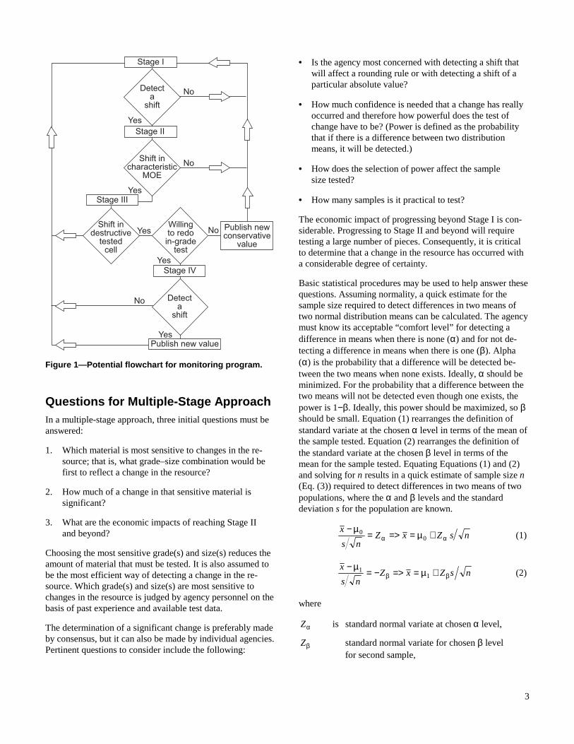
Figure 1 shows an example of a potential system for themultiple-stage approach. In Stage I, a nondestructive testprogram is conducted on what is anticipated to be the mostsensitive grade and size combination. This stage may havemultiple steps to further decrease sample size. Steps aredefined as repeated sampling on a regular or periodic basis.Stage II is reached if the most sensitive grade–size combina-tion indicated that a change in properties had occurred.Change is defined as a targeted shift of x amount in a prop-erty. The term trigger level describes the property value levelassociated with the targeted shift. The trigger level is definedas the original property value of the sample minus thetargeted shift amount.

In Stage II, additional tests (destructive or nondestructive)are conducted on one or more sizes and grades to confirmthat the trigger level has been reached. If the targeted shift isnot confirmed, the original periodic testing of Stage I isreinitiated. If the targeted shift is confirmed in Stage II, afurther stage of destructive testing in the full range of grade–size combinations may be initiated.

3

Questions for Multiple-Stage ApproachIn a multiple-stage approach, three initial questions must beanswered:

1. Which material is most sensitive to changes in the re-source; that is, what grade–size combination would befirst to reflect a change in the resource?

2. How much of a change in that sensitive material issignificant?

3. What are the economic impacts of reaching Stage IIand beyond?

Choosing the most sensitive grade(s) and size(s) reduces theamount of material that must be tested. It is also assumed tobe the most efficient way of detecting a change in the re-source. Which grade(s) and size(s) are most sensitive tochanges in the resource is judged by agency personnel on thebasis of past experience and available test data.

The determination of a significant change is preferably madeby consensus, but it can also be made by individual agencies.Pertinent questions to consider include the following:

• Is the agency most concerned with detecting a shift thatwill affect a rounding rule or with detecting a shift of aparticular absolute value?

• How much confidence is needed that a change has reallyoccurred and therefore how powerful does the test ofchange have to be? (Power is defined as the probabilitythat if there is a difference between two distributionmeans, it will be detected.)

• How does the selection of power affect the samplesize tested?

• How many samples is it practical to test?

The economic impact of progressing beyond Stage I is con-siderable. Progressing to Stage II and beyond will requiretesting a large number of pieces. Consequently, it is criticalto determine that a change in the resource has occurred witha considerable degree of certainty.

Basic statistical procedures may be used to help answer thesequestions. Assuming normality, a quick estimate for thesample size required to detect differences in two means oftwo normal distribution means can be calculated. The agencymust know its acceptable “comfort level” for detecting adifference in means when there is none (α) and for not de-tecting a difference in means when there is one (β). Alpha(α) is the probability that a difference will be detected be-tween the two means when none exists. Ideally, α should beminimized. For the probability that a difference between thetwo means will not be detected even though one exists, thepower is 1−β. Ideally, this power should be maximized, so βshould be small. Equation (1) rearranges the definition ofstandard variate at the chosen α level in terms of the mean ofthe sample tested. Equation (2) rearranges the definition ofthe standard variate at the chosen β level in terms of themean for the sample tested. Equating Equations (1) and (2)and solving for n results in a quick estimate of sample size n(Eq. (3)) required to detect differences in two means of twopopulations, where the α and β levels and the standarddeviation s for the population are known.

nsZxZns

xαα +µ==>=

µ−0

0 (1)

nsZxZns

xββ +µ==>−=

µ−1

1 (2)

where

αZ is standard normal variate at chosen α level,

βZ standard normal variate for chosen β levelfor second sample,

Stage I

Stage II

Stage III

Yes

No

Yes

Yes

Yes

Publish new value

Publish newconservative

value

Detecta

shift

Stage IV

Willingto redoin-grade

test

Shift indestructive

testedcell

No

No

Yes

Shift incharacteristic

MOE

Detecta

shift

No

Figure 1—Potential flowchart for monitoring program.

4

n sample size,

s common standard deviation of two populations,

µ0 average value of original population,

µ1 average value of new sample to be detected(trigger level),

x value of sample average above which nodifference is declared, and

µ0 − µ1 magnitude of change to be observed(targeted shift).

Setting Equation (1) = Equation (2) gives sample size n:

( )( )

2

µ−µ

+−=

10

β sZZn

α (3)

Figure 2 illustrates the effect of selecting different α and βlevels. For example, if the agency is monitoring MOE, it maywant to limit the chance of falsely detecting a change inMOE to 5% (α = 0.05, αZ = −1.645) and to set the probabil-

ity of proceeding to Stage II to 50% if there is a change inMOE (β = 0.5, βZ = 0) (Fig. 2a). This is quite different

from setting criteria so that there is 90% probability of de-tecting that MOE has shifted (Fig. 2b). Parts (c) and (d) ofFigure 2 provide examples of 95% and 99% assurance,respectively, that MOE has shifted.

There are further complications, however, to choosing aparticular α or β level on MOE for monitoring structuralproperties. The true concern is not only whether MOE haschanged, but also how this change affects other mechanicalproperties. Existing information can be used to make as-sumptions about the relationship between other propertiesand MOE. However, it is preferable to run a number ofsimulations, making use of real strength and stiffness data, toprovide a clearer understanding of the potential variabilityand sensitivity of a multiple-stage monitoring program. Therest of this report provides simulated results based on theNorth American In-Grade test data for Southern Pine and thespecific example of the monitoring program initiated bySPIB. The simulated results are dependent on the MOE–MOR relationship observed during the In-Grade testprogram. If this relationship itself is altered, the simulationresults may not be valid.

H0: µ1 = µ0H1: µ1 < µ0

Fre

quen

cy

(a)

Estimated MOE

α β

Power50%

x

Fre

quen

cy

(c)

α β

Power95%

0 µ1 µ0

Estimated MOE0 µ1 µ0

x

Zα = �1.645Zβ = 0

Zα = �1.645Zβ = 1.645

Fre

quen

cy

(b)

Estimated MOE

α β

Power90%

x

Fre

quen

cy

(d)

α β

Power99%

0 µ1 µ0

Estimated MOE0 µ1 µ0

x

Zα = �1.645Zβ = 1.28

Zα = �1.645Zβ = 2.33

1�β = Power

Figure 2—Differences in selection of α and β levels.

5

Simulations

DataThe data used in the simulations were the SPIB In-Grade testresults (Green and Evans 1987). The test data were adjustedusing the procedures outlined in ASTM D1990 that arecurrently used to calculate the allowable properties listed inthe American Forest & Paper Association (AF&PA) NationalDesign Specification (NDS) for Wood Construction(AF&PA 1997).

MethodsSimulations were conducted in two phases. In Phase 1, weexamined the impact of different sample sizes on the abilityto predict changes in properties. In Phase 2, we investigatedthe sensitivity of MOE as a monitoring parameter by simu-lating potential scenarios of future resource changes.

Phase 1Phase 1 investigated the likelihood of falsely predictingtargeted shifts in properties when no change had occurred inthe data set for a range of sample sizes. A program wasdeveloped to randomly select monitoring samples from theexisting In-Grade data sets for bending with no changes. Theproperties considered were MOE and MOR. All trials lookedat data randomly selected from either the entire data set orwithin each geographic region, weighting by productionpercentages. The use of closed-form solutions was also in-vestigated.

Phase 2Phase 2 addressed the sensitivity of the monitoring techniqueto detect predetermined changes in strength properties

(trigger levels) with one to three steps. Targeted shifts inMOE were investigated. A targeted shift is a change of aspecific amount x in MOE. The corresponding values ofMOR were adjusted in accordance with MOE–MOR regres-sion equations determined from the original In-Grade South-ern Pine data.

In a number of simulations, regression equations were usedto evaluate possible shifts of concern. Required sample sizesto detect a given change in MOE were investigated. Also,possible shifts in MOE caused by increases in juvenile woodwere simulated.

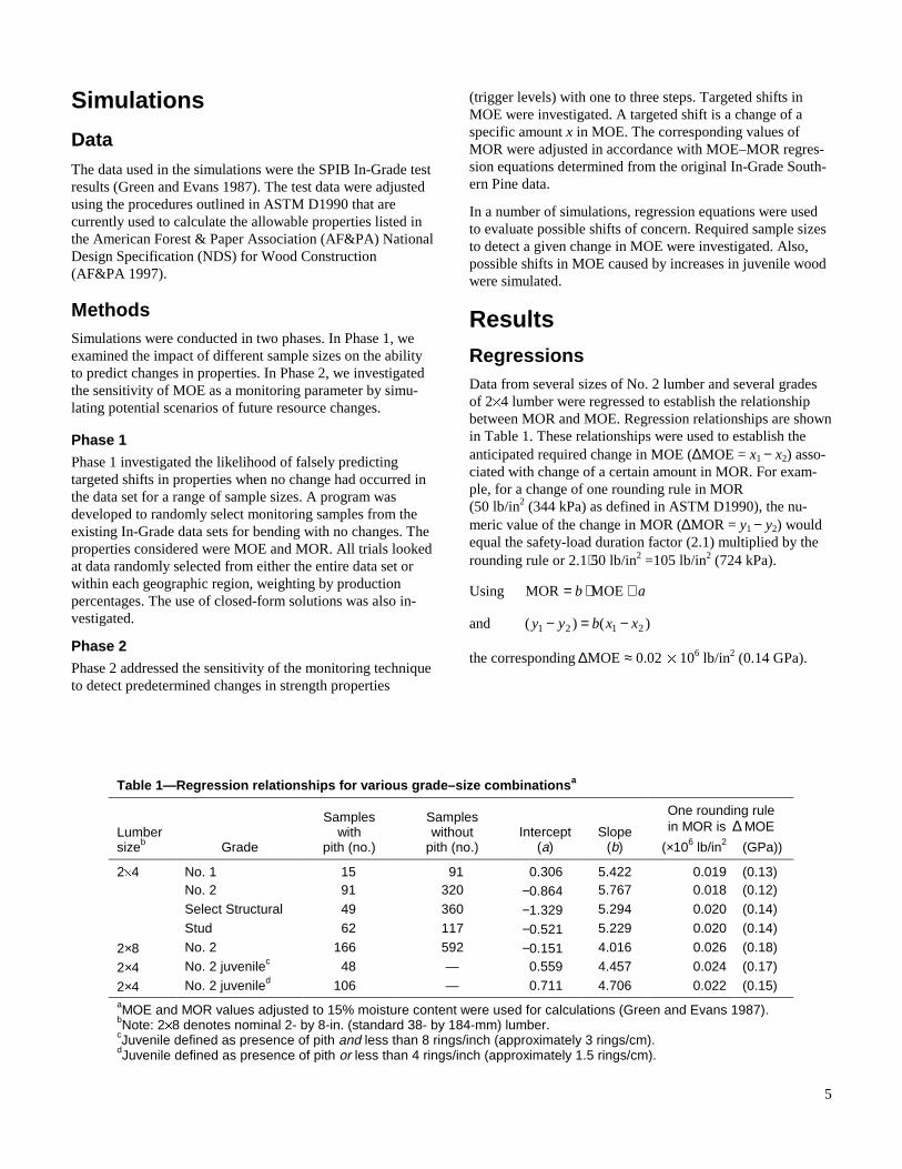
ResultsRegressionsData from several sizes of No. 2 lumber and several gradesof 2�4 lumber were regressed to establish the relationshipbetween MOR and MOE. Regression relationships are shownin Table 1. These relationships were used to establish theanticipated required change in MOE (∆MOE = x1 − x2) asso-ciated with change of a certain amount in MOR. For exam-ple, for a change of one rounding rule in MOR(50 lb/in2 (344 kPa) as defined in ASTM D1990), the nu-meric value of the change in MOR (∆MOR = y1 − y2) wouldequal the safety-load duration factor (2.1) multiplied by therounding rule or 2.1⋅50 lb/in2 =105 lb/in2 (724 kPa).

Using ab +⋅= MOEMOR

and )()( 2121 xxbyy −=−

the corresponding 02.0MOE ≈∆ � 106 lb/in2 (0.14 GPa).

Table 1—Regression relationships for various grade–size combinations a

One rounding rulein MOR is ∆ MOELumber

sizeb Grade

Sampleswith

pith (no.)

Sampleswithout

pith (no.)Intercept

(a)Slope

(b) (×106 lb/in2 (GPa))

2�4 No. 1 15 91 0.306 5.422 0.019 (0.13)No. 2 91 320 −0.864 5.767 0.018 (0.12)Select Structural 49 360 −1.329 5.294 0.020 (0.14)Stud 62 117 −0.521 5.229 0.020 (0.14)

2×8 No. 2 166 592 −0.151 4.016 0.026 (0.18)

2×4 No. 2 juvenilec 48 — 0.559 4.457 0.024 (0.17)

2×4 No. 2 juveniled 106 — 0.711 4.706 0.022 (0.15)aMOE and MOR values adjusted to 15% moisture content were used for calculations (Green and Evans 1987).bNote: 2�8 denotes nominal 2- by 8-in. (standard 38- by 184-mm) lumber.cJuvenile defined as presence of pith and less than 8 rings/inch (approximately 3 rings/cm).dJuvenile defined as presence of pith or less than 4 rings/inch (approximately 1.5 rings/cm).

6

There is considerable variability about the MOE–MORregression relationships for lumber but a well-establishedcorrelation (Green and Kretschmann 1991). For the sizes andgrades considered, one rounding rule in MOR correspondsto, on average, a change in MOE of approximately 0.02 �

106 lb/in2 (0.14 GPa). Using defined juvenile wood data sets,

one rounding rule in MOR corresponds to a change in MOEof 0.025 � 106 lb/in2 (0.17 GPa). These changes in MOEare much smaller than the rounding rule change of0.1 � 106 lb/in2 (0.69 GPa) in ASTM D1990.

Sample SizeThe effect of sample size on the percentage of false positivereadings, for one rounding rule in MOE and MOR (Table 2)and three targeted shifts in MOE (0.1, 0.025, and 0.02, Ta-bles 3 to 5, respectively), was investigated using 100,000simulated samples for each case. For each sample, a failurewas considered to have occurred when the average MOE orthe 5th percentile MOR for the sample was below the respec-tive trigger level for the property. The MOE trigger level wasthe original mean MOE minus the targeted shift of onerounding rule of 0.1 � 106 lb/in2 (0.69 GPa). For a samplesize of 50 and a change in MOE of 0.1 � 106 lb/in2

(0.69 GPa), when two successive sample failures are requiredthere is a 0.033% chance of falsely declaring a shift in MOE(Table 2). The MOR trigger level was the original MOR 5th

percentile minus 50 lb/in2 (344 kPa). For the same example,there is a 23% chance of a false indication of a shift in MOR.

In Table 2, a step represents one complete sample of mate-rial. In the example just described, one step represents thesurvey of data from 1 year. Step 2 represents sampling fromthe next year and so on. For the MOE and MOR data incolumns 3 and 4, “overall” designates samples selectedrandomly, with replacement, from all of the original 413 2�4Select Structural (SS) pieces until the test sample was ob-tained. The number of No. 2 2�4 pieces tested in the In-Grade program was 413. The second run (columns 5 and 6)

was a repeat of the original overall simulation. “Regionalselection” designates material sampled randomly from withina given region, proportional to production in that region,until the 413-piece sample was reached.

The results shown in Table 2 suggested that the false positiverates for the two overall simulations were not substantiallydifferent than those for the regional selection. Therefore, therest of the tests were run using random selection from theoverall database.

Tables 3 to 5 compare the effect of sample size on thechances of falsely detecting a change in MOE for three levelsof change in MOE (0.1, 0.025, and 0.020 � 106 lb/in2

(0.69 GPa, 0.17 GPa, 0.14 GPa), respectively). If multiplesteps are used, these results suggest little difference betweensample sizes of 1000, 413, or 200. If the sample size is below200, there is a significant increase in the chance of falsepositive readings.

The results of these simulations demonstrate the importanceof sampling method in regard to the sample size required. Ifan agency were dependent on the information gathered overonly 1 year (that is, one step), then the sample size requiredto reduce the chance of detecting false positive below 1% fora change in MOE of 0.025 would usually be well over 1,000specimens (Table 4). This same level of confidence can bereached with slightly more than 200 specimens after threesteps have been taken. For a random sample size, repeatedsampling (multiple-stage approach) helps to ensure that adetected shift is not a result of the natural variability of therandom sample by reducing the chances of falsely detecting aproperty shift. The original In-Grade grade–size sample of413 pieces is very unlikely to give a false positive indicationof a shift for MOE in a multiple-step process. The samplesize simulation results in Tables 2 to 5 also suggest thatdetection with three steps and a sample size of 200 is roughlyequivalent to a two-step procedure with a sample size of 413.

Table 2—Probability of falsely detecting change of one rounding rule a when no change had occurred

Probability (%)Overall Second run of overall Regional selection

Sample size Step MOE MOR MOE MOE MOR MOR

50 1 1.76 48.0 1.75 47.8 1.31 47.72 0.033 23.0 0.41 22.9 0.016 22.8

200 1 0 34.4 0.001 34.3 0.001 31.92 0 11.9 0 11.8 0 10.2

413 1 0 27.1 0 26.9 0 26.92 0 7.3 0 7.2 0 7.3

1,000 1 0 17.5 0 17.6 0 14.52 0 3.1 0 3.1 0 2.1

aRounding rule defined as 0.1 × 106 lb/in2 (0.69 GPa) in MOE or 50 lb/in2 (344 kPa) in MOR.

7

Therefore, a smaller sample size could be used with moresteps to detect a targeted shift in MOE. A sample size of atleast 360 should be considered to obtain good representationof all geographic regions. Also, if a shift in MOE of onerounding rule is observed, a shift of several rounding rulesmay have occurred for MOR.

Juvenile WoodIncreases in the percentage of juvenile wood in a piece weresimulated in three ways. In each simulation, the criteria fordefining the presence of juvenile wood were presence orabsence of pith and number of rings per unit length, with4 rings/inch equal to approximately 1.5 rings/cm.

Simulation 1 Presence of pith

Simulation 2 Presence of pith and <4 rings/inchAbsence of pith or ≥4 rings/inch

Simulation 3 Presence of pith or <4 rings/inchAbsence of pith and ≥4 rings/inch

The effects of these three sets of sorting criteria on MOE andMOR are illustrated in Tables 6, 7, and 8, respectively. In-formation on the presence or absence of pith was not avail-able for all of the original In-Grade samples. Therefore, thetotal number of pieces listed by presence or absence of pithmay not equal the actual number of pieces tested.

Table 3—Probability of falsely detecting 0.1 �� 106 lb/in 2

(0.69 GPa) change in MOE when no change hadoccurred

Probability (%)

Sample size Step

2x4No. 2

2x4SSa

2x4Stud

2x8No. 2

50 1 2.964 1.665 3.223 4.377

2 0.092 0.019 0.088 0.193

3 0.005 0 0.004 0.009

100 1 0.381 0.120 0.411 0.746

2 0.004 0 0.001 0.010

3 0 0 0 0

200 1 0.009 0.001 0.015 0.036

2 0 0 0 0

3 0 0 0 0

413 1 0 0 0 0.001

2 0 0 0 0

3 0 0 0 0

1000 1 0 0 0 0

2 0 0 0 0

3 0 0 0 0aSS is Select Structural.

Table 4— Probability of falsely detecting0.025 �� 106 lb/in 2 (0.17 GPa) change in MOE when nochange had occurred for various sizes and grades (%)

Probability (%)

Sample size Step

2x4No. 2

2x4SS

2x4Stud

2x8No. 2

50 1 33.571 29.481 32.690 34.155

2 11.235 8.811 10.725 11.679

3 3.754 2.722 3.517 4.032

100 1 27.369 22.267 26.122 27.877

2 7.411 4.875 6.893 7.839

3 2.028 1.095 1.797 2.182

200 1 19.788 13.972 18.173 20.234

2 3.932 1.911 3.271 4.033

3 0.776 0.286 0.604 0.785

413 1 11.087 5.990 9.420 11.359

2 1.189 0.344 0.877 1.319

3 0.142 0.016 0.086 0.154

1000 1 2.832 0.741 2.130 3.009

2 0.051 0.007 0.054 0.088

3 0 0 0.002 0.003

Table 5—Probability of falsely detecting 0.02 �� 106 lb/in 2

(0.14 GPa) change in MOE when no change hadoccurred

Probability (%)

Sample size Step

2x4 No. 2

2x4SS

2x4Stud

2x8No. 2

50 1 37.137 33.283 36.123 37.329

2 13.729 11.256 13.056 13.965

3 5.028 3.832 4.727 5.291

100 1 32.108 27.065 30.663 32.014

2 10.176 7.269 9.470 10.310

3 3.286 1.988 2.928 3.304

200 1 25.476 19.257 23.335 25.458

2 6.498 3.666 5.448 6.349

3 1.641 0.704 1.286 1.576

413 1 17.204 10.545 14.689 16.819

2 2.891 1.082 2.106 2.776

3 0.480 0.111 0.332 0.435

1000 1 7.148 2.582 5.193 6.630

2 0.458 0.060 0.293 0.425

3 0.033 0 0.017 0.020

8

For Simulation 1, MOR values for No. 2 lumber were notvery sensitive to the presence of pith (Table 6). This wasprobably caused by the exclusion of some pieces with largerknots from the pith group when pieces were selected on thebasis of pith alone. However, for all grades, MOE was sensi-tive to changes in the presence of pith. We concluded thatdefining juvenile wood on the basis of presence of pith andthe number of rings per unit length resulted in too few piecesfor a proper simulation. Therefore, for the remaining simula-tions, presence of pith was used as the criterion for juvenilewood.

Changes in properties were simulated using random samplingwith discarding. Increases in the percentage of pieces withjuvenile wood were simulated by discarding pieces that didnot meet the criteria defining juvenile wood. Thus, for a 20%

discard rate, if a piece were drawn that did not meet thejuvenile wood definition (that is, a piece without pith), itwould be discarded from the sample 20% of the time. Notethat this is different from requiring certain percentages ofpieces with juvenile wood in the sample. The 20%, 40%,60%, and 80% discard rate sample sets were established bydiscarding, with that probability, pieces without pith andreplacing those pieces by resampling the original 413-piecesample. The resampled pieces did or did not have pith.

Table 9 lists the random sampling results for SS 2�4 lumberfor various properties when the discard rate was increased.An example is given for each property simulated to demon-strate how the boundaries were established for various com-parisons of the 100,000 simulation samples.

Table 6—Effect of Simulation 1 sorting criteria on MOE and MOR

Mean MOE 5th percentile MORLumbersize Grade Sorting criteria

Samplesize (x106 lb/in2 (GPa)) (x103 lb/in2 (MPa))

2�4 SS All 409 1.823 (12.6) 6.987 (48.2)With pith 49 1.660 (11.4) 4.996 (34.4)Without pith 360 1.845 (12.7) 7.121 (49.1)

2�4 No. 2 All 411 1.534 (10.6) 3.842 (26.5)With pith 91 1.334 (9.2) 3.835 (26.4)Without pith 320 1.591 (11.0) 3.821 (26.3)

2�4 Stud All 179 1.487 (10.3) 3.246 (22.4)With pith 62 1.356 (9.3) 2.908 (20.1)Without pith 117 1.556 (10.7) 3.798 (26.2)

2�8 No. 2 All 758 1.543 (10.6) 2.584 (17.8)With pith 166 1.464 (10.1) 2.473 (17.1)Without pith 592 1.566 (10.8) 2.588 (17.0)


Mean MOE 5th percentile MORLumber

size Grade Sorting criteriaaSample

size (x106 lb/in2 (GPa)) (x103 lb/in2 (MPa))

2�4 SS All 409 1.823 (12.6) 6.987 (48.2)With pith and <4 rpi 1 1.490 (10.3) — (—)Without pith or >4 rpi 408 1.824 (12.6) 6.983 (48.1)

No. 2 All 411 1.534 (10.6) 3.842 (26.5)With pith and <4 rpi 5 0.971 (6.7) 3.575 (24.6)Without pith or >4 rpi 406 1.541 (10.6) 3.863 (26.6)

2�4 Stud All 179 1.487 (10.3) 3.246 (22.4)With pith and <4 rpi 9 0.967 (6.7) 2.901 (20.0)Without pith or >4 rpi 170 1.515 (10.4) 3.405 (23.5)

2�8 No. 2 All 758b 1.543 (10.6) 2.584 (17.8)With pith and <4 rpi 36 1.153 (7.9) 2.473 (17.1)Without pith or >4 rpi 721 2.584 (17.8) 2.588 (17.8)

arpi is rings per inch; 4 rpi is approximately 1.5 rings/cm.bOne piece was eliminated from study as result of lack of information on both pith and rings per unit length.

9

Example Simulations

MOE SimulationIn Table 10, the boundary for MOE is the average MOE(1.823 � 106 lb/in2 (12.6 GPa), Table 6) of the original In-Grade SS 2�4 sample minus 0.025 � 106 lb/in2 (0.17 GPa) or1.798 � 106 lb/in2 (12.4 GPa). For step 1 (the first 413-piecesample), the average MOE was determined and comparedagainst 1.798 � 106 lb/in2 (12.4 GPa). A failure was consid-ered to have occurred if this average value was less than theboundary MOE; 5,990 of 100,000 samples had averagesbelow the boundary (Table 10). Step 2 represents the numberof times that two failures occurred in a row. Thus, if a failurehad already occurred and the average MOE of the next sam-ple of 413 pieces fell below the boundary, one piece wasadded to the total of failures for step 2. If the average MOEof the subsequent sample was above 1.798 � 106 lb/in2

(12.4 GPa), no step 2 failure had occurred and the compari-son was conducted the next time when the average MOE ofa 413-piece sample fell below the boundary.

For the 99,999 samples checked, there were 344 occurrenceswhen two samples in a row had an average MOE below the

boundary by chance with no discard. The same process wasused for three samples in a row. For SS 2�4, there were only16 occurrences when three samples in a row had an averageMOE < 0.025 � 106 lb/in2 (<0.17 GPa) less than the averageMOE of the original sample when no change in populationhad occurred (that is, no pieces had been discarded). As thediscard rate increased (that is, increase in percentage ofpieces with juvenile wood), the percentage of failuresdetected with repeated samplings (steps 1 to 3) increaseddramatically.

MOR SimulationIn Table 10, the boundary used for MOR was the safety-loadduration factor of 2.1 times one rounding rule (2.1 � 50 = 105lb/in2 (723 kPa)) subtracted from the 5th percentile (6.987 �103 lb/in2 (48.2 MPa)). The actual value of the SS 2�4 MORboundary was 6.882 � 103 lb/in2 (47.5 MPa). For each 413-piece sample, the 5th percentile MOR was determined andcompared to this boundary. The regression relationship inTable 1 was used to determine what an equivalent change inMOE would be with a rounding rule change in MOR.


Mean MOE 5th percentile MORLumbersize Grade Sorting criteria

Samplesize (x106 lb/in2 (GPa)) (x103 lb/in2 (MPa))

2�4 SS All 409 1.823 (12.6) 6.987 (48.2)

With pith or <4 rpi 53 1.654 (11.4) 4.662 (32.1)

Without pith and >4 rpi 356 1.848 (12.7) 7.230 (49.9)

2�4 No. 2 All 411 1.514 (10.4) 3.842 (26.5)

With pith or <4 rpi 106 1.314 (9.1) 3.879 (26.7)


2�4 Stud All 179 1.487 (10.3) 3.246 (22.4)

With pith or <4 rpi 78 1.303 (9.0) 2.893 (19.9)


2�8 No. 2 All 758 1.543 (10.6) 2.584 (17.8)

With pith or <4 rpi 274 1.416 (9.8) 2.391 (16.5)


Table 9—Effect of discard rate on properties and pith a

Property No discard 20% discard 40% discard 60% discard 80% discard

Pith range 25–78 32–95 42–113 68–147 126–218

Pith mean 49 59 76 104 166

MOE mean (x106 lb/in2 (GPa)) 1.824 (12.6) 1.819 (12.5) 1.812 (12.5) 1.799 (12.4) 1.771 (12.2)

MOR 5% (x103 lb/in2 (MPa)) 6.939 (47.8) 6.873 (47.4) 6.769 (46.7) 6.589 (45.4) 6.290 (45.4)aData from 2�4 SS sample. Sample size = 413. Target MOE = 0.025 � 106 lb/in2 (0.17 GPa).

10

From Table 10, of 100,000 samples, there were 35,830 oc-currences when the calculated MOR 5th percentile was belowthe boundary. For the 99,999 samples checked in step 2,there were 12,847 occurrences when two samples in a rowhad a calculated MOR 5th percentile below the boundary.Finally, for the 99,998 samples checked in step 3, there were4,564 occurrences when three samples in a row had a calcu-lated MOR 5th percentile below the boundary.

Pith SimulationA binomial distribution was used to determine a one-sidedupper 95% confidence interval for the expected number ofspecimens discarded, based on the lack of pith in a 413-piecesample. Equation (4) was used to calculate the bounds of the95% confidence interval,

+±

nn

pqpn

2

1645.1 (4)

where p is the probability a specimen has pith, q is 1 − p, andn is sample size.

The continuity correction factor (1/2n) was ignored becausethe large sample sizes made it negligible. The upper bound-ary for the confidence interval was used for both pith andproof-load simulations. Using the upper boundary ensureda high level of confidence that the shift had in fact occurred

and was not merely observed as a result of chance. We wereinterested in the side of the interval where there would be toomany, rather than too few, pieces with pith or proof-loadfailures.

In the original In-Grade SS 2�4 sample, 49 of 413 piecescontained pith:

413881.0)1(119.0413

49 ==−=== npqp (5)

Equation (5) can be written in terms of pieces containingpith:

81.5981.1049413

364

413

49413645.1

413

49413 =+=⋅⋅+ (6)

Therefore, the boundary for pith that should be used is( ) ≅⋅+ 413026.049 60. In this case, a “failure” was said to

occur if �60 pieces in the 413-piece sample contained pith.From Table 10, 5,837 of 100,000 samples had �60 pieceswith pith. However, in only 371 of 99,999 occurrences didtwo sample sets in a row have �60 pieces with pith, and inonly 19 of 99,998 occurrences did three sample sets in a rowhave �60 pieces with pith.

Table 10—Percentage of failures in average MOE, MOR, pith, or proof load observedat different steps for various discard rates a

Failures (%)

Property Step No discard 20% discard 40% discard 60% discard 80% discard

MOEb 1 5.990 10.337 20.788 48.501 94.892

2 0.344 1.060 4.290 23.451 90.029

3 0.016 0.110 0.899 11.385 85.449

MORc 1 35.830 46.116 51.586 82.899 98.664

2 12.847 21.188 37.864 68.706 97.347

3 4.564 9.645 23.259 56.932 96.047

Pithd 1 5.837 49.221 98.278 100 100

2 0.371 24.115 96.583 100 100

3 0.019 11.833 94.915 100 100

Proof loade 1 4.800 8.146 15.931 36.270 82.205

2 0.232 0.676 2.533 13.088 67.489

3 0.012 0.060 0.434 4.688 55.372aSimulation based on 2�4 SS sample. Sample size = 413.bTarget MOE = 1.798 � 106 lb/in2 (12.4 GPa).cTarget MOR = 6.882 lb/in2 � 103 lb/in2 (47.4 MPa).dTarget number of pieces with pith >60.eTarget order statistic >27th order.

11

Proof-Loading SimulationProof loading is a process of loading a member to a selectedlevel to obtain “proof” that the member will perform at thatload level. For wood, proof loading is usually used to deter-mine which samples pass a 5th percentile criterion for astrength property. To simulate the effect of proof loading, thecomparison boundary was determined again by using a bi-nomial function. Using the 5th percentile definition andEquation (4), the upper 95% confidence limit boundary wasdetermined to be anything greater than the 27th order statisticof the MOR of the original 413-piece SS 2�4 sample. There-fore, a “failure” was considered to have occurred if the MORof �28 of 413 pieces was less than that of the targeted proof-load:

9.27286.765.20

95.005.0413645.105.0413

=+=⋅⋅+⋅

(7)

Tables 11 to 13 present results similar to those presented inTables 8 to 10 for different grades and sizes and a samplesize of 413. The results suggest that proof-load testing forMOR is not a meaningful monitoring scheme when a shift inMOR is linked to a shift in MOE because monitoring forMOE is more powerful. Also, using the presence of pith todetect a change in resource may be overly sensitive to shifts

in MOE but may have potential as an early detection mecha-nism for property shifts. However, pith sensitivity variesfrom cell to cell.

The results of these simulations show that several steps areneeded to limit the probability of detecting a shift in MOEwhen one does not truly exist. In Tables 6 and 9 and theupper part of Table 11, results on the effect of discard rate onproperties and presence of pith show that for a given changein MOE, there may be several rounding rule changes in MORfor higher grade lumber and few changes for low-gradematerial. If MOR is chosen as the monitoring property, thesimulations suggest that shifts in MOR can be detected eas-ily. Monitoring of MOR may also be grade dependent. MOE,on the other hand, seems to be quite grade-independent anddoes not give as high a rate of false declarations of a change.Therefore, MOE is a better monitoring property than isMOR.

MOE Trigger LevelsThe MOE trigger is the amount of a shift in MOE that isacceptable prior to initiating Stage II testing. To determinehow the discard rate affected the percentage of samplesresulting in a MOE shift of a particular magnitude, we con-sidered MOE shifts of 0.02, 0.04, 0.05, and 0.1 � 106 lb/in2

(0.14, 0.28, 0.34, and 0.69 GPa, respectively). The resultsare listed in Tables 14 and 15.

Table 11—Effect of discard rate on properties and presence of pith and percentage of failuresin No. 2 2 ×4 sample for various discard rates a

Effect of discard rate

Pith or property Step No discard 20% discard 40% discard 60% discard 80% discard

Pith range — 56–125 72–150 95–174 131–220 200–286

Pith mean — 91 108 132 171 242

MOE mean (x106 lb/in2 (GPa)) — 1.530 (10.5) 1.520 (10.5) 1.505 (10.4) 1.482 (10.2) 1.438 (9.9)

MOR 5% (x103 lb/in2 (MPa)) — 3.845 (26.5) 3.845 (26.5) 3.846 (26.5) 3.848 (26.5) 3.851 (26.6)

Failures (%)

MOE 1 11.087 25.775 57.339 93.604 99.997

2 1.189 6.662 32.978 87.616 99.993

3 0.142 1.674 18.857 82.024 99.989

MOR 1 12.730 12.180 11.100 9.743 7.597

2 1.640 1.541 1.265 0.926 0.564

3 0.191 0.207 0.151 0.079 0.038

Pith 1 5.759 64.222 99.859 100 100

2 0.341 41.371 99.717 100 100

3 0.015 26.652 99.576 100 100

Proof load 1 4.850 4.682 4.203 3.772 3.142

2 0.233 0.231 0.193 0.118 0.093

3 0.011 0.008 0.008 0.003 0.003aTarget MOE = 0.025 � 106 lb/in2 (0.17 GPa).

12

Table 12—Effect of discard rate on properties and presence of pith and percentage of failures in 2×4 Studsample for various discard rates a



Pith range 99–182 125–213 149–243 193–279 258–338

Pith mean 143 165 194 235 300

MOE mean (x106 lb/in2 (GPa)) 1.487 (10.3) 1.477 (10.2) 1.463 (10.1) 1.442 (9.9) 1.411 (9.7)

MOR 5% (x103 lb/in2 (MPa)) 3.245 (22.4) 3.205 (22.1) 3.161 (21.8) 3.106 (21.4) 3.036 (20.9)

Failures (%)

MOE 1 9.420 22.259 49.941 86.200 99.790

2 0.877 4.930 24.994 74.345 99.579

3 0.086 1.080 12.501 64.124 99.368

MOR 1 30.704 36.401 44.172 55.774 71.189

2 9.455 13.308 19.672 31.279 50.718

3 2.871 4.810 8.746 17.551 36.063

Pith 1 5.565 72.856 99.977 100 100

2 0.323 53.027 99.953 100 100

3 0.016 38.605 99.929 100 100

Proof load 1 2.078 2.999 4.872 8.735 18.033

2 0.049 0.088 0.215 0.760 3.254


Table 13—Effect of discard rate on sample properties and presence of pith and percentage of failures in No. 82×4 sample for various discard rates a



Pith range 56–131 70–149 93–171 123–218 201–284

Pith mean 91 107 132 170 241

MOE mean (x106 lb/in2 (GPa) 1.543 (10.6) 1.539 (10.6) 1.533 (10.6) 1.524 (10.5) 1.506 (10.4)

MOR 5% (x103 lb/in2 (MPa)) 2.580 (17.8) 2.577 (17.8) 2.573 (17.7) 2.567 (17.7) 2.553 (17.6)

Failures (%)

MOE 1 11.359 15.635 23.490 39.599 72.754

2 1.319 2.403 5.491 15.604 52.912

3 0.154 0.359 1.268 6.126 38.407

MOR 1 7.772 8.870 10.895 14.250 21.724

2 0.602 0.760 1.187 2.003 4.676

3 0.040 0.066 0.127 0.286 1.030

Pith 1 4.950 61.591 99.844 100 100

2 0.247 37.948 99.689 100 100

3 0.011 23.499 99.534 100 100

Proof load 1 5.186 5.490 6.021 6.850 8.531

2 0.272 0.309 0.365 0.446 0.722


13

Table 14—Effect of discard rate on likelihood of detecting given targeted shift in MOE for SS 2x4 sample a

Effect of discard rate for various MOE means

No discard 20% discard 40% discard 60% discard 80% discard

MOE shift(x106 lb/in2 (GPa)) Step

1.824 ×106 lb/in2

(12.6 GPa)

1.819 ×106 lb/in2

(12.5 GPa)

1.812 ×106 lb/in2

(12.5 GPa)

1.799 ×106 lb/in2

(12.4 GPa)

1.771 ×106 lb/in2

(12.2 GPa)

0.02 (0.14) 1 10.545 16.9 30.338 60.375 97.357

2 1.082 2.846 9.235 36.389 94.776

3 0.111 0.469 2.821 21.878 92.273

0.04 (0.28) 1 0.635 1.445 4.102 17.020 76.828

2 0.006 0.021 0.172 2.947 58.983

3 0 0.002 0.005 0.496 45.318

0.05 (0.34) 1 0.083 0.257 0.985 6.025 55.308

2 0 0 0.007 0.336 30.640

3 0 0 0 0.024 16.902

0.10 (0.69) 1 0 0 0 0 0.194

2 0 0 0 0 0

3 0 0 0 0 0

aSample size = 413.

Table 15—Effect of discard rate on likelihood of detecting given targeted shift in MOE for No. 2 2x4 sample a

Effect of discard rate for various MOE means

No discard 20% discard 40% discard 60% discard 80% discard

MOE shift(x106 lb/in2 (GPa)) Step

1.530 ×106 lb/in2

(10.5 GPa)

1.520 ×106 lb/in2

(10.5 GPa)

1.505×106 lb/in2

(10.4 GPa)

1.482×106 lb/in2

(10.2 GPa)

1.438 ×106 lb/in2

(9.9 GPa)

0.02 (0.14) 1 17.204 35.523 67.899 96.445 100

2 2.891 12.601 46.120 93.011 100

3 0.480 4.431 31.283 89.705 100

0.04 (0.28) 1 1.990 6.899 25.467 75.225 99.933

2 0.029 0.479 6.506 56.600 99.865

3 0.001 0.026 1.628 42.576 99.797

0.05 (0.34) 1 0.443 2.043 11.149 54.673 99.622

2 0 0.038 1.246 30.017 99.245

3 0 0.001 0.125 16.417 98.871

0.10 (0.69) 1 0 0 0.007 0.302 39.460

2 0 0 0 0.001 15.634

3 0 0 0 0 6.161

aSample size = 413.

14

Implications of SimulationsThe simulations indicate that “what if” scenarios can beconsidered using normal statistics and existing data insteadof further simulations. If a constant is subtracted from theMOE of every piece (Fig. 3), the probability that a test willpick up that difference can be calculated. Equation (8) givesthe standard normal variate )(1 β−Z for detecting an actual

shift of a given amount based on various targeted shifts.

nZ

σshift actual targeted

)(1−=β− (8)

Table 16 shows the likelihood of detecting a given actualshift in MOE if the targeted shift is set at different levels. Ifthe actual shift equals the targeted shift, there is a 50%chance of detecting the change. As the actual shift increasesor decreases with respect to the targeted shift, there is anincrease or decrease in the likelihood of detecting it. Thisclearly indicates that there is very little chance that a minorshift in MOE would be detected if the trigger level were setto detect a targeted shift of 0.1 � 106 lb/in2 (0.69 GPa).

Using Equation (9), the random chance of detecting a shiftwhen none had occurred for a given targeted shift is given inTable 17.

nZ

σshift actual targeted

)(−=α (9)

These values, based on normal distribution statistics, arecomparable to those presented in Tables 2 to 5, which werebased on simulations. This information has been used as aguide in developing a resource monitoring program at theSouthern Pine Inspection Bureau (SPIB).

SPIB Resource MonitoringProgramThe SPIB has conducted a resource monitoring programannually since 1994. This program was developed as a means

of recognizing whether a significant change has occurred inlumber strength properties. Both the SPIB Technical Com-mittee and Board of Governors have shown solid support forthis program since its inception.

Method of SamplingMills are selected in a similar fashion to that used in theoriginal North American In-Grade program (Green andothers 1989). Each SPIB mill is assigned to a geographicregion and the production from each region is totaled. Basedon the proportion of production from each region, the num-ber of pieces to be selected from that region is calculated.The target minimum sample size is 360 pieces. Regardless ofthe actual number of pieces required for a given region, aminimum sample size of 10 pieces/mill and a maximum of15 pieces/mill were established. Because of the minimumsample size per mill, the actual sample size has ranged fromyear to year from 380 to 405 pieces. Each year, approxi-mately 30 mills are randomly selected from all of the SPIBsubscriber mills that produce No. 2 2�4 lumber (SPIB 1994).Because of timing issues related to reporting productionfigures and scheduling data collection for the monitoringprogram, the regional production percentages are based onthe annual production figures 2 years prior to the testing. Theselection of mills to be sampled is conducted by the ForestProducts Laboratory. The mills in each region are randomlyranked. The appropriate number of mills is then selected toobtain the required sample size for each region.

The data collected for each piece include width, thickness,length, moisture content, rings/inch, estimated percentage oflatewood, grade-controlling characteristic, maximumstrength-reducing characteristic, and two MOE values deter-mined using a Metriguard E-Computer (Metriguard, Pull-man, WA) . The E-Computer is calibrated using an 8-lb(3.6 kg) brass weight, and the theoretical constant (79.4) tomaintain the “true, dynamic E” is used. All data are collectedat the individual mill sites. Ambient and wood temperaturedata are also collected, and an effort is made to test the woodat temperatures above 32°F (0°C).

After the data are collected for each annual program, severaldata adjustments are made. First, the two E-Computer Evalues are averaged to obtain a single value for each piece.Because the E-Computer assumes nominal dimensions (thatis, 2�4 is 1.5 by 3.5 in.), the average E value is adjusted forthe actual dimensions of each piece. The E value is furtheradjusted for moisture content to 15% using the moisturecontent model in ASTM D1990.

In a separate, unpublished study conducted by SPIB, theissue of adjusting a flatwise, E-Computer E value to beequivalent to an edgewise, static bending E value was con-sidered. Data were from a 1994 machine-stress-rated (MSR)tension test program. The sample consisted of 2�4 to 2�10lumber with a total sample size of 140 pieces. The

Fre

quen

cy

0 µ1 µ0Estimated MOE

Targetedshift

Actualshift H0:µ1 = µ0

H1:µ1 < µ0

Figure 3—Illustration of shifts in MOE.

15

Table 16—Likelihood of detecting actual shift for various targeted shifts for 2 ��4 samples

Likelihood (%) of detecting actual MOE shift for targeted shifts

Grade

Actual shiftin MOE

(x106 lb/in2

(GPa))

–0.1 x106 lb/in2

(–0.69 GPa)

–0.05 x106 lb/in2

(–0.34 GPa)

–0.04 x106 lb/in2

(–0.28 GPa)

–0.025 x106 lb/in2

(–0.17 GPa)

–0.02 x106 lb/in2

(–0.14 GPa)

SS Mean µ0 1.824 (12.6)σ 0.332 (2.3)n 413 –0.15

(–1.0)99.9 100.0 100.0 100.0 100.0

–0.125(–0.86)

93.7 100.0 100.0 100.0 100.0

–0.1(–0.69)

50.0 99.9 99.9 100.0 100.0

–0.05(–0.34)

0.1 50.0 72.9 93.7 96.7

–0.04(–0.28)

0 27.1 50.0 82.1 88.9

–0.025(–0.17)

0 6.3 17.9 50.0 62.2

–0.02(–0.14)

0 3.3 11.1 37.8 50.0

–0.01(–0.07)

0 0.7 3.3 17.9 27.1

No. 2 Mean µ0 1.531 (10.6)σ 0.366 (2.5)n 413 –0.15

(–1.0)99.7 100.0 100.0 100.0 100.0

–0.125(–0.86)

91.8 100.0 100.0 100.0 100.0

–0.1(–0.69)

50.0 99.7 99.7 100.0 100.0

–0.05(–0.34)

0.3 50.0 71.2 91.8 95.3

–0.04(–0.28)

0 28.8 50.0 79.7 86.7

–0.025(–0.17)

0 8.2 20.3 50.0 61.0

–0.02(–0.14)

0 4.8 13.4 39.0 50.0

–0.01(–0.07)

0 1.3 4.8 20.3 28.8

Table 17—Likelihood of detecting targeted shift when no shift had occurred for 2 ��4 samples

Actual shift Likelihood (%) of detecting actual MOE shift for targeted shifts

Grade

in MOE(x106 lb/in2

(GPa))

–0.1 x106 lb/in2

(–0.69 GPa)

–0.05 x106 lb/in2

(–0.34 GPa)

–0.04 x106 lb/in2

(–0.28 GPa)

–0.025 x106 lb/in2

(–0.17 GPa)

–0.02 x106 lb/in2

(–0.14 GPa)

SS Mean µ0 1.824(12.6)

σ 0.332(2.3)

0 0.1 0.7 6.3 11.1

n 413No. 2 Mean µ0 1.531

(10.6)σ 0.366

(2.5)0 0.3 1.3 8.2 13.4

n 413

16

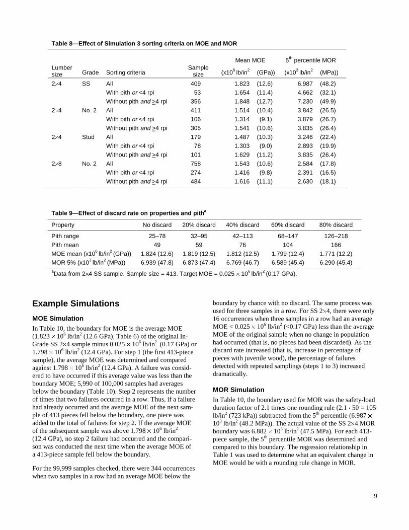
E-Computer E value was the average of two lengthwiseorientations. Information on edgewise static E was collectedfrom a Metriguard 312 proof loader using a 21:1 span todepth ratio. The results are plotted in Figure 4.

The data showed that for E values less than about2.0 � 106 lb/in2 (13.8 GPa), a slight upward adjustment to theE-computer E value would be appropriate; for E valuesgreater than 2.0 � 106 lb/in2 (13.8 GPa), a slight downwardadjustment would be appropriate. No adjustment was madeto convert E-Computer E values to edgewise E values be-cause average E of the SPIB resource monitoring programdata was less than 2.0 � 106 lb/in2 (13.8 GPa) and it would beconservative to not make an adjustment.

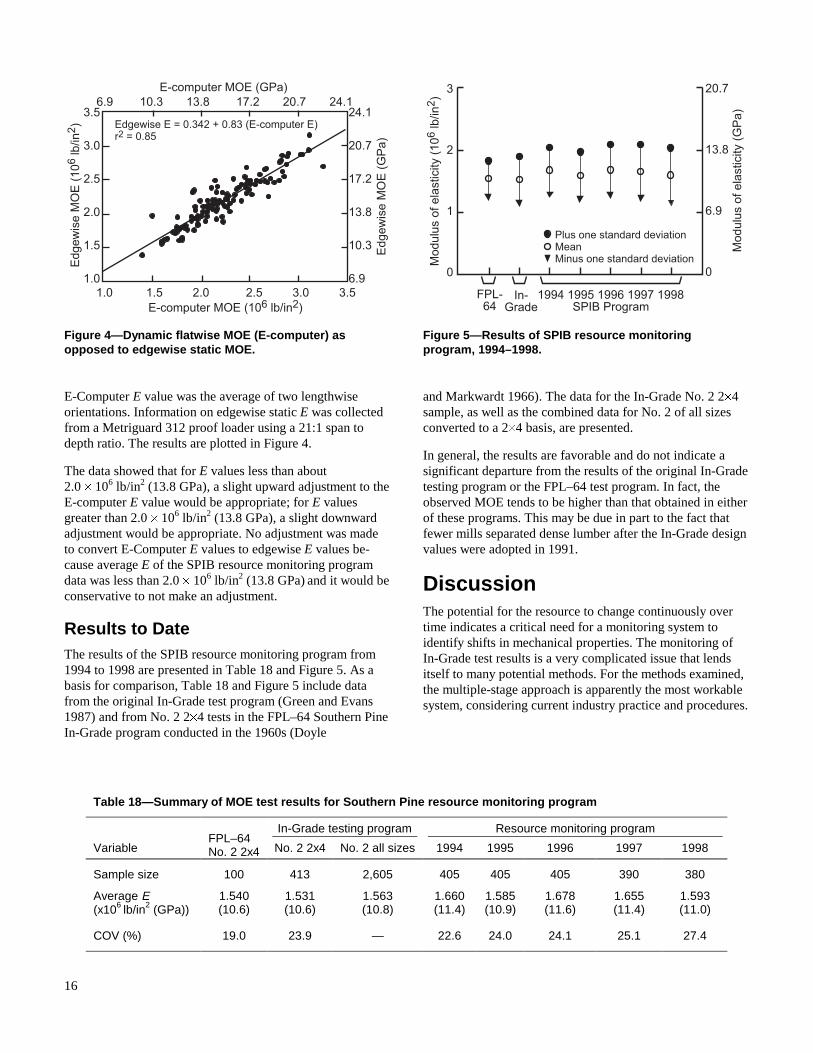
Results to DateThe results of the SPIB resource monitoring program from1994 to 1998 are presented in Table 18 and Figure 5. As abasis for comparison, Table 18 and Figure 5 include datafrom the original In-Grade test program (Green and Evans1987) and from No. 2 2�4 tests in the FPL–64 Southern PineIn-Grade program conducted in the 1960s (Doyle

and Markwardt 1966). The data for the In-Grade No. 2 2�4sample, as well as the combined data for No. 2 of all sizesconverted to a 2�4 basis, are presented.

In general, the results are favorable and do not indicate asignificant departure from the results of the original In-Gradetesting program or the FPL–64 test program. In fact, theobserved MOE tends to be higher than that obtained in eitherof these programs. This may be due in part to the fact thatfewer mills separated dense lumber after the In-Grade designvalues were adopted in 1991.

DiscussionThe potential for the resource to change continuously overtime indicates a critical need for a monitoring system toidentify shifts in mechanical properties. The monitoring ofIn-Grade test results is a very complicated issue that lendsitself to many potential methods. For the methods examined,the multiple-stage approach is apparently the most workablesystem, considering current industry practice and procedures.

3.5

3.0

2.5

2.0

1.5

1.0

Edg

ewis

e M

OE

(10

6 lb

/in2 )

24.1

20.7

17.2

13.8

10.3

6.9

Edg

ewis

e M

OE

(G

Pa)

Edgewise E = 0.342 + 0.83 (E-computer E)r2 = 0.85

E-computer MOE (106 lb/in2)1.0 1.5 2.0 2.5 3.0 3.5

E-computer MOE (GPa)6.9 10.3 13.8 17.2 20.7 24.1

Figure 4—Dynamic flatwise MOE (E-computer) asopposed to edgewise static MOE.

3

2

1

0

Mod

ulus

of e

last

icity

(10

6 lb

/in2 )

FPL-64

Plus one standard deviationMeanMinus one standard deviation

20.7

13.8

6.9

0

Mod

ulus

of e

last

icity

(G

Pa)

1994 1995 1996 1997 1998SPIB Program

In-Grade

Figure 5—Results of SPIB resource monitoringprogram, 1994–1998.

Table 18—Summary of MOE test results for Southern Pine resource monitoring program

In-Grade testing program Resource monitoring program

VariableFPL–64No. 2 2x4 No. 2 2x4 No. 2 all sizes 1994 1995 1996 1997 1998

Sample size 100 413 2,605 405 405 405 390 380

Average E(x106 lb/in2 (GPa))

1.540(10.6)

1.531(10.6)

1.563(10.8)

1.660(11.4)

1.585(10.9)

1.678(11.6)

1.655(11.4)

1.593(11.0)

COV (%) 19.0 23.9 — 22.6 24.0 24.1 25.1 27.4

17

The multiple-stage approach, with multiple steps at Stage I,allows for small sample sizes with a high probability that theselected trigger level is truly a change and did not occur byrandom chance. The program initiated by the Southern PineInspection Bureau is a fine initial attempt at monitoringstructural lumber. Ultimately, the decision of the best methodfor determining changes in the resource lies in the hands ofthe various grading agencies responsible for supervising theimplementation of the current visual grading rules.

There is a definite need for more study of monitoring possi-bilities. Additional work is needed to assess more fully theeconomic impact of not recognizing a true shift in properties.For example, if there is a concern that a change in the re-source will primarily increase the coefficient of variability(COV) of material properties, then a lower tail (that is, 5th

percentile value MOE) might be more sensitive to thatchange. Other simulations could be conducted with existingdata to examine the impact of changes in production, such asincreases in MSR production at dimension mills, changes inmarkets, or changing variability on reliability-based designcalculations. Finally, a large representative study of planta-tion material could be collected across the growth range ofthe Southern Pine sample to obtain an accurate picture of theimpact of rapid growth on properties.

We hope that the most important impact of this publicationwill be to provide a framework for discussing various optionsof monitoring properties. We envision that this documentwill serve as the starting point for determining appropriatemethods for monitoring structural lumber.

ConclusionsThe simulations demonstrated the relative sensitivity of amultiple-stage monitoring approach to sample size, juvenilewood content, and selected trigger levels:

Differences in a uniform shift in MOE detected by monitor-ing procedures may be explained as clearly in closed-formsolutions based on normal distributions as by simulations.

The targeted shift of MOE should be less than0.1 � 106 lb/in2 (0.69 GPa).

For smaller target shifts, it is better to use a multiple-stepprocess to confirm any observed shifts.

A sample size of approximately 400 is very unlikely to give afalse positive indication of a shift for MOE after three steps.

Depending on the current relationship between MOE andMOR, if a shift of one rounding rule in MOE is detected, it ispossible that many shifts in a rounding rule for MOR mayhave occurred, particularly in the higher lumber grades.

A multiple-stage approach can be smoothly implemented bya grading agency as part of its regular quality controlprogram.

ReferencesAF&PA. 1997. Design values for wood construction—asupplement to the 1997 edition of the National DesignSpecification. Washington, DC: American Forest & PaperAssociation.

ASTM. 1997. Annual book of standards. Vol. 04.10. Wood.ASTM D1990–97. Standard practice for establishing allow-able properties for visually-graded dimension lumber fromin-grade tests of full-size specimens. West Conshohocken,PA: American Society for Testing and Materials: p. 287.

Barrett, J.D.; Kellogg, R.M.. 1989. Strength and stiffness ofdimension lumber. Second growth Douglas-fir: its managementand conversion for value. Forintek Canada Corporation.SP–32 ISSN 0824–2119. April: 50–58. Chapter 5.

Bendtsen, B.A.; Senft, J. 1986. Mechanical and anatomicalproperties in individual growth rings of plantation-growneastern cottonwood and loblolly pine. Wood and FiberScience.18(1): 23–38.

Bendtsen, B. Alan; Plantinga, Pamela L.;. Snellgrove,Thomas A. 1988. The influence of juvenile wood on themechanical properties of 2x4’s cut from Douglas-fir planta-tions. In: Proceedings of the 1988 International Conferenceon Timber Engineering. Vol. 1.

Biblis, E.J. 1990. Properties and grade yield of lumber froma 27-year-old slash pine plantation. Forest Products Journal.40(3): 21–24.

Bier, H.; Collins, M.J. 1984. Bending properties of 100 x50 mm structural timber from a 28-year-old stand of NewZealand radiata pine. IUFRO Group S5.02. Xalapa, Mexico.New Zealand Forest Service Reprint 1774. December.

Boone, R.S.; Chudnoff, M. 1972. Compression wood for-mation and other characteristics of plantation-grown Pinuscaribaea. Res. Pap. ITF–13. Rio Piedros, Puerto Rico: U.S.Department of Agriculture, Forest Service, Institute ofTropical Forestry.

Clarke III, A;. Saucier, J.R. 1989. Influence of initialplanting density, geographic location and species on juvenilewood formation in southern pine. Forest Products Journal.39(7/8): 42–48.

Doyle, D.V; Markwardt, L.J. 1966. Properties of SouthernPine in relation to strength grading of dimension lumber.Res. Pap. FPL–64. Madison, WI: U.S. Department of Agri-culture, Forest Service, Forest Products Laboratory.

Green, D.W; Evans J.W. 1987. Mechanical properties ofvisually graded lumber: Vol. 1–8. Springfield VA: NationalTechnical Information Service. U.S. Department ofCommerce. PB–88–159–371.

18

Green, D.W.; Kretschmann, D.E. 1991. Lumber propertyrelationships for engineering design standards. Wood andFiber Science. 23(3): 436–456.

Green, D.W.; Shelley, B E.; Vokey H.P. 1989. In-gradetesting of structural lumber. In: Proceedings of workshopsponsored by In-grade Testing Committee and Forest Prod-ucts Society. FPS Proceedings 47363. Madison, WI: ForestProducts Society.

Johnson, R A.; Evans J.W.; Green, D.W. 1995. Predictivedistribution of order statistics. In: Balakrishnan, N., ed.Recent advances in life-testing and reliability. Boca Raton:CRC Press: 505–521.

Johnson, R.A.; Evans J.W.; Green, D.W. 1999. Non-parametric Bayesian predictive distributions for future orderstatistics. Statistics and Probability Letters. 41: 247–254.

Kretschmann, D.E.; Bendtsen, B.A. 1992. Ultimate tensilestress and modulus of elasticity of fast-grown plantationloblolly pine lumber. Wood and Fiber Science. 24(2):189–203.

MacPeak, Malcolm D.; Burkart, L.F.; Weldon, D. 1990.Comparison of grade, yield, and mechanical properties oflumber produced from young fast-grown and older slow-grown planted slash pine. Forest Products Journal.40(1): 11–314.

Montgomery D.C. 1997. Introduction to statistical qualitycontrol. 3d ed. New York, NY: John Wiley and Sons, Inc.

Pearson, R.G. 1984. Characteristics of structural importanceof clear wood and lumber from fast-grown loblolly pinestands. In: Proceedings, on utilization of the changing woodresource in the Southern United States;1984 June 12–13;North Carolina State University, Raleigh, NC

Pearson, R.G.; Gilmore, R.C. 1971. Characterization of thestrength of juvenile wood of loblolly pine. Forest ProductsJournal. 21(1): 23–30.

Smith, I.; Alkan, S.; Chui, Y.H. 1991. Variation of dy-namic properties and static bending strength of a plantationgrown red pine. Journal of Institute of Wood Science.12(4): 221–224.

Southern Pine Inspection Bureau. 1994. Standard gradingrules. Pensacola, FL: Southern Pine Inspection Bureau.

Walford, G.B. 1982. Current knowledge of the in-gradebending strength of New Zealand radiata pine. FRI Bull. 15.New Zealand.

Ying, L.; Kretschmann, D.E.; Bendtsen, B.A. 1994. Lon-gitudinal shrinkage in fast-grown loblolly pine plantationwood. Forest Products Journal. 44(1): 58–62.

Documents

Monitoring of visually graded structural lumber