Monitoring the impacts of vertebrate pest control … the impacts of vertebrate pest control operations on non-target wildlife species DEPARTMENT OF CONSERVATION TECHNICAL SERIES 24

Monitoring the impacts ofvertebrate pest control operationson non-target wildlife species

DEPARTMENT OF CONSERVATION TECHNICAL SERIES 24

E.B. Spurr and R.G. Powlesland

Published by

Department of Conservation

P.O. Box 10-420

Wellington, New Zealand

Department of Conservation Technical Series presents instructional guide books and data sets, aimed

at the conservation officer in the field. Publications in this series are reviewed to ensure they represent

standards of current best practice in the subject area.

This publication originated from work done under Department of Conservation Investigation no. 2331,

carried out by E.Spurr (Landcare Research, PO Box 69, Lincoln, New Zealand), and R. Powlesland

(Department of Conservation, Science and Research Unit, PO Box 10-420, Wellington, New Zealand).

Publication was approved by the Manager, Science & Research Unit, Science Technology and

Information Services, Department of Conservation, Wellington.

© May 2000, Department of Conservation

ISSN 1172�6873

ISBN 0�478�21955�5

Cataloguing in Publication

Spurr, Eric B.

Monitoring the impacts of vertebrate pest control operations on non-

target wildlife species / E.B. Spurr and R. G. Powlesland. Wellington,

N.Z. : Dept. of Conservation, 2000.

1 v. ; 30 cm. (Department of Conservation technical series,

1172-6873 ; 24).

Includes bibliographical references.

ISBN 0478219555

1. Animal populations�New Zealand�Effect of pest control on.

2. Invertebrates�New Zealand�Effect of pesticides on. I. Powlesland,

Ralph G. (Ralph Graham), 1952- II. Title. III. Series: Department of

Conservation technical series ; 24).

CONTENTS

Abstract 5

1. Introduction 6

2. Bait quality 6

2.1 Fresh bait 6

2.2 Weathered bait 8

2.3 Interpretation of results 8

3. Monitoring impacts on non-target species 8

3.1 Experimental design 9

3.2 Replication and randomness of treatment allocation 9

3.3 Power 10

3.4 Statistical analysis 11

4. Birds 13

4.1 Five-minute counts 13

4.2 Territory-mapping (or roll-calling) 20

4.3 Mist-netting capture rates 23

4.4 Banding and recapturing or resighting 24

4.5 Radio-telemetry 26

4.6 Other techniques 28

5. Bats 28

5.1 Counts of bats leaving and/or entering daytime roosts 28

5.2 Counts of �bat passes� recorded by bat detectors 29

5.3 Radio-telemetry 30

6. Reptiles 31

6.1 Pitfall trapping 31

6.2 Minimum number alive 32


7. Frogs 34

7.1 Strip transect counts 35


8. Fish 37

9. Invertebrates 37

9.1 Pitfall trapping 37

9.2 Litter sampling 39

9.3 Malaise trapping 40

9.4 Counts of invertebrates feeding on baits 41


4

10. Dead animals 43

10.1 Collection of samples 43

10.2 Packaging, storage, and transport 44

10.3 Interpretation of results 45

11. Water samples 46

12. Recommendations 46

13. Acknowledgements 46

14. References 47

5

Abstract

This publication gives protocols for determining bait quality, monitoring the

impacts of pest control operations on populations of non-target species (birds,

bats, reptiles, frogs, fish, and invertebrates), and collecting tissues from dead

animals and samples of water for toxicity testing. Some of the protocols are still

being developed (e.g. protocols for monitoring bats and frogs). Users of these

protocols should consult with relevant experts before starting a monitoring

programme. We recommend that the Department of Conservation call meetings

of relevant experts to finalise the development of standard methods for

monitoring the population trends of various wildlife species.

Keywords: pest control, 1080 poisoning, brodifacoum, monitoring, non-target

species, birds, bats, reptiles, frogs, fish, invertebrates, water samples

6

1. Introduction

A recent review (Spurr & Powlesland 1997) highlighted the need for protocols

for monitoring the impacts (costs and benefits) of aerial 1080-poisoning

operations for control of the brushtail possum (Trichosurus vulpecula) on

populations of non-target wildlife species. There is also a need for protocols for

monitoring the impacts of other poisons for control of other pests (e.g. the

impacts of brodifacoum-poisoning operations for eradication of rodents on non-

target wildlife species on offshore islands), and for monitoring the impacts of

ongoing pest control using a variety of methods in mainland islands. These

protocols should be used in conjunction with the Vertebrate Pest Control

Manual (Haydock & Eason 1997) and Best Current Practices in Sequential Use of

Possum Baits (Henderson et al. 1998), which describe the properties of

different poisons and protocols for carrying out pest control operations. The

protocols will need reviewing and updating as methods develop.

2. Bait quality

Aspects of bait quality that affect non-target species include factors such as bait

size, toxicant concentration, colour, cinnamon concentration, and hardness.

For example, baits containing a lot of small pieces (�chaff� or �dust�) pose a risk

to small forest birds (Harrison 1978; Powlesland et al. 1999). Baits containing

1080 are dyed green to reduce their attractiveness to birds (Caithness &

Williams 1971). Cinnamon oil is added to baits partly to mask the smell and taste

of 1080 to possums (Morgan 1990) and partly to repel birds (Udy and Pracy

1981). Specifications for these factors are given in the Vertebrate Pest Control

Manual (Haydock & Eason 1997). Baits should be checked that they meet these

specifications before they are applied in the field (see below). Toxicant

concentration may also be checked at various times after the bait has been

applied in the field (e.g. to determine whether the bait is still toxic to non-target

species). When handling toxic baits follow the appropriate Health and Safety

procedures for handling pesticides (e.g. wear gloves). When transporting toxic

baits refer to the relevant Standard Operating Procedures (e.g. baits need to be

securely held, not in the driver�s cabin, attended to at all times, kept separate

from food and drink, and accounted for). The following instructions were

adapted from G.R.G. Wright (Landcare Research pers. comm.).

2 . 1 F R E S H B A I T

2.1.1 Carrot bait

Carrot bait containing 1080 should be checked for size, toxicant concentration,

colour, and cinnamon concentration. Samples of bait should be collected on the

7

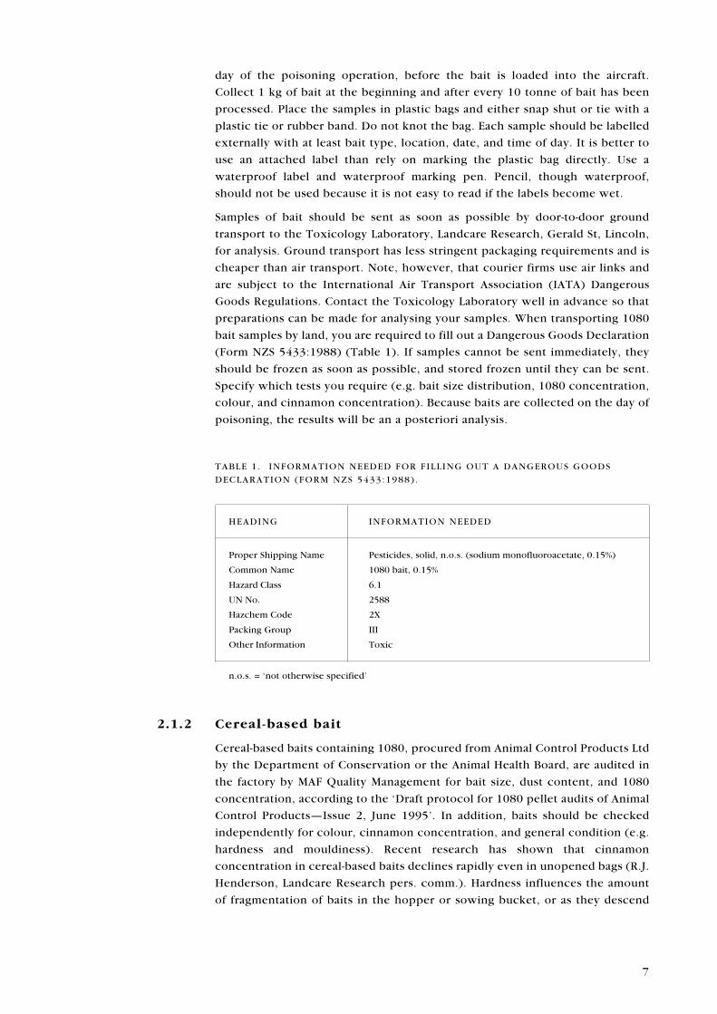
day of the poisoning operation, before the bait is loaded into the aircraft.

Collect 1 kg of bait at the beginning and after every 10 tonne of bait has been

processed. Place the samples in plastic bags and either snap shut or tie with a

plastic tie or rubber band. Do not knot the bag. Each sample should be labelled

externally with at least bait type, location, date, and time of day. It is better to

use an attached label than rely on marking the plastic bag directly. Use a

waterproof label and waterproof marking pen. Pencil, though waterproof,

should not be used because it is not easy to read if the labels become wet.

Samples of bait should be sent as soon as possible by door-to-door ground

transport to the Toxicology Laboratory, Landcare Research, Gerald St, Lincoln,

for analysis. Ground transport has less stringent packaging requirements and is

cheaper than air transport. Note, however, that courier firms use air links and

are subject to the International Air Transport Association (IATA) Dangerous

Goods Regulations. Contact the Toxicology Laboratory well in advance so that

preparations can be made for analysing your samples. When transporting 1080

bait samples by land, you are required to fill out a Dangerous Goods Declaration

(Form NZS 5433:1988) (Table 1). If samples cannot be sent immediately, they

should be frozen as soon as possible, and stored frozen until they can be sent.

Specify which tests you require (e.g. bait size distribution, 1080 concentration,

colour, and cinnamon concentration). Because baits are collected on the day of

poisoning, the results will be an a posteriori analysis.

2.1.2 Cereal-based bait

Cereal-based baits containing 1080, procured from Animal Control Products Ltd

by the Department of Conservation or the Animal Health Board, are audited in

the factory by MAF Quality Management for bait size, dust content, and 1080

concentration, according to the �Draft protocol for 1080 pellet audits of Animal

Control Products�Issue 2, June 1995�. In addition, baits should be checked

independently for colour, cinnamon concentration, and general condition (e.g.

hardness and mouldiness). Recent research has shown that cinnamon

concentration in cereal-based baits declines rapidly even in unopened bags (R.J.

Henderson, Landcare Research pers. comm.). Hardness influences the amount

of fragmentation of baits in the hopper or sowing bucket, or as they descend

TABLE 1 . INFORMATION NEEDED FOR FILLING OUT A DANGEROUS GOODS

DECLARATION (FORM NZS 5433:1988) .

HEADING INFORMATION NEEDED

Proper Shipping Name Pesticides, solid, n.o.s. (sodium monofluoroacetate, 0.15%)

Common Name 1080 bait, 0.15%

Hazard Class 6.1

UN No. 2588

Hazchem Code 2X

Packing Group III

Other Information Toxic

n.o.s. = �not otherwise specified�

8

through the forest canopy to the ground. Methods of measuring hardness are

still being developed. Samples of 1 kg of bait should be collected from four bags

selected at random, and sent to the Toxicology Laboratory, Landcare Research,

Gerald St, Lincoln. Specify which tests you require (e.g. colour, cinnamon

concentration). A Dangerous Goods Declaration (Form NZS 5433:1988) is

required, as above, when transporting baits containing 1080.

Cereal-based baits containing brodifacoum, pindone, or cholecalciferol should

also be checked to determine whether they meet specifications. This analysis

can be done at the Toxicology Laboratory, Landcare Research, Gerald St,

Lincoln. The Hazard Class, UN No.; Hazchem Code, and Packing Group for

transportation of these baits have not been allocated.

2 . 2 W E A T H E R E D B A I T

Samples of weathered baits (carrots and cereal-based baits) are sometimes

collected from the field to assess residual concentrations of toxicants. A total of

10�50 g of bait is required for a single analysis. Each sample should be put into

a separate plastic bag or container, and labelled with bait type, location, and

date. The samples should be sent by the quickest method of ground transport to

the Toxicology Laboratory, Landcare Research, Gerald St, Lincoln, using the

same transport details as for fresh bait. If the samples cannot be sent

immediately, they should be stored in a freezer until they can be sent. A

Dangerous Goods Declaration (Form NZS 5433:1988) is required, as above, for

any baits containing 1080.

2 . 3 I N T E R P R E T A T I O N O F R E S U L T S

The report from Landcare Research will state the mean and 95% confidence

limits of the toxicant concentration in the baits, plus the limits of detection. If

requested, the bait size distribution, cinnamon concentration, etc. will also be

given. These data can be compared to the bait specifications given in the

Vertebrate Pest Control Manual (Haydock & Eason 1997).

3. Monitoring impacts on non-target species

Issues to consider when planning to monitor the impacts of vertebrate pest

control operations on non-target species include experimental design,

replication, randomness, power, and methods of analysis. As a general rule, a

biometrician should always be consulted when planning a monitoring

programme.

9

3 . 1 E X P E R I M E N T A L D E S I G N

The experimental design should be appropriate to the situation. The best design

for monitoring the impacts of a treatment such as vertebrate pest control on

non-target species is to measure the population density (or an index of

population density) of the non-target species in treatment and non-treatment

areas before and after treatment is applied in the treatment area (Green 1979).

The sampling plots (or lines) should be randomly located within each area, or

within strata within each area (i.e. stratified random sampling). If possible,

measurements should be made at the same plots (or lines) after treatment as

before treatment. This design assumes that the trends in non-target species

populations in the two areas would, in the absence of treatment, change in a

similar way with time. The design has been used extensively to monitor the

effects of vertebrate pest control on bird populations in mainland forests (e.g.

Spurr 1981, 1988, 1991; Powlesland et al. 1999).

An alternative design is to measure populations before and after treatment only

in the treatment area (i.e. there is no non-treatment area). This assumes that

there are no natural changes with time (e.g. no seasonal changes in behaviour

and no differences in weather) that might affect population estimation (from

counting or trapping animals). This design has been used to monitor the effects

of vertebrate pest control on bird populations on offshore islands where it is

difficult to establish non-treatment areas (e.g. Miller & Anderson 1992;

Robertson et al. 1993; Towns et al. 1993; Empson & Miskelly 1999; Robertson &

Colbourne in press).

Another design is to measure populations in treatment and non-treatment areas

only after treatment has been applied (i.e. there is no before-treatment

assessment). This design assumes that the populations in the two areas were

similar before treatment. It has not been used yet to measure the impacts of

vertebrate pest control on non-target species.

3 . 2 R E P L I C A T I O N A N D R A N D O M N E S S O F

T R E A T M E N T A L L O C A T I O N

To be able to generalise the results, a minimum of two replicates is required

(i.e. at least two treatment areas and/or two non-treatments areas). Plots (or

lines) within treatment and non-treatment areas are not replicates but are sub-

samples (or pseudo-replicates in the sense of Hurlbert 1984), and are used to

obtain a more accurate population estimate in each area. True replicates are

different pest control operations that occur at the same time and that use the

same bait type, toxicant concentration, application rate, etc. However, this is

usually not possible when assessing the impact of vertebrate pest control. There

is usually only one control operation to assess at a time. Consequently, the

results apply only to that control operation.

To be statistically valid, in addition to replication, the area(s) receiving

treatment should be assigned at random. Again, this is not possible for

vertebrate pest control. The areas receiving treatment are always �selected�

because of high pest numbers. Non-treatment areas usually have lower pest

10

numbers. This cannot be avoided. Nevertheless, non-treatment areas should be

selected with habitat and wildlife as similar as possible to the treatment areas.

In the following sections, it is assumed that there is only one treatment and one

non-treatment area, that the treatment area is not randomly selected, that plots

(or lines) within areas are randomly located, and that both treatment and non-

treatment areas are monitored before and after pest control.

3 . 3 P O W E R

If data are available from previous surveys using the same techniques, then a

priori power analyses should be done to determine the power of the proposed

survey to detect a given change in population abundance, should one occur, or

to determine the number of samples required to detect a given change in

population abundance for a given power (Green 1994). If previous data are not

available, the new data obtained should be used to determine the sample sizes

required (for a given power) to detect changes in population abundance in

future surveys.

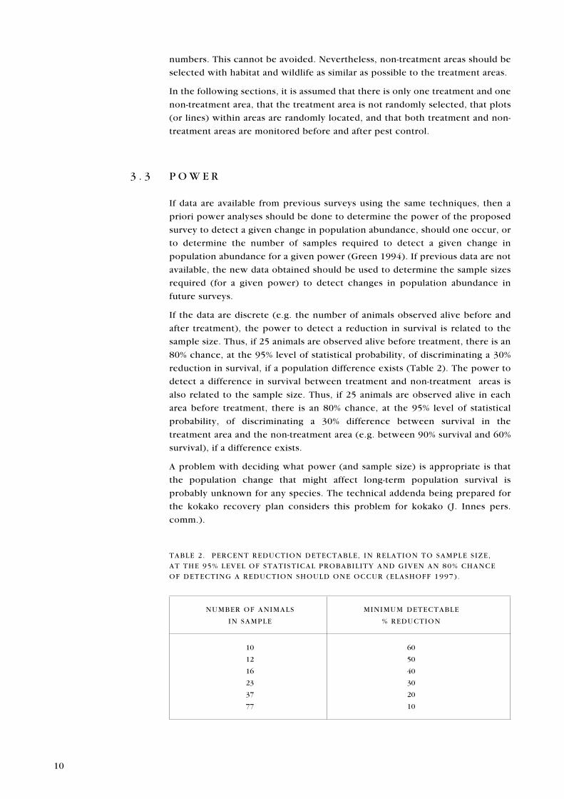
If the data are discrete (e.g. the number of animals observed alive before and

after treatment), the power to detect a reduction in survival is related to the

sample size. Thus, if 25 animals are observed alive before treatment, there is an

80% chance, at the 95% level of statistical probability, of discriminating a 30%

reduction in survival, if a population difference exists (Table 2). The power to

detect a difference in survival between treatment and non-treatment areas is

also related to the sample size. Thus, if 25 animals are observed alive in each

area before treatment, there is an 80% chance, at the 95% level of statistical

probability, of discriminating a 30% difference between survival in the

treatment area and the non-treatment area (e.g. between 90% survival and 60%

survival), if a difference exists.

A problem with deciding what power (and sample size) is appropriate is that

the population change that might affect long-term population survival is

probably unknown for any species. The technical addenda being prepared for

the kokako recovery plan considers this problem for kokako (J. Innes pers.

comm.).

TABLE 2 . PERCENT REDUCTION DETECTABLE, IN RELATION TO SAMPLE S IZE,

AT THE 95% LEVEL OF STATISTICAL PROBABILITY AND GIVEN AN 80% CHANCE

OF DETECTING A REDUCTION SHOULD ONE OCCUR (ELASHOFF 1997) .

NUMBER OF ANIMALS MINIMUM DETECTABLE

IN SAMPLE % REDUCTION

10 60

12 50

16 40

23 30

37 20

77 10

11

3 . 4 S T A T I S T I C A L A N A L Y S I S

3.4.1 Comparison of population trends in treatment and non-treatment areas

Where there is replication of treatments, and random allocation of which areas

are treatment areas and which are non-treatment areas, and where

measurements of non-target species populations in the treatment and non-

treatment areas are repeated at the same plots before and after treatment, the

appropriate test to determine the impact of treatment is the repeated measures

analysis of variance (Green 1993). The test can be done using a statistical

package such as SYSTAT® (SPSS 1996). The data should be checked for

normality and, if needed, transformed with square-root or loge (x+1). If the data

are transformed for analysis, the sample means and standard errors should be

back-transformed for graphing. In the analysis, the effect of treatment is

indicated by the treatment × time interaction term, for which the statistical

package will produce an exact P value. As noted above, this requires at least two

treatment areas and/or two non-treatment areas, measured at least once before

and after treatment. However, most assessments of pest control operations are

unreplicated, and treatments are not randomly allocated to treatment areas.

Without replication and random allocation of treatments, the population

estimates before and after treatment in treatment and non-treatment areas can

be compared by a repeated measures analysis of variance with the number of

plots (or lines) in each area as the sample size, provided the plots (or lines) are

independent and have been randomly located. Such an analysis will indicate

whether there has been an area × time interaction (as distinct from a treatment

× time interaction), but it cannot determine the cause of any interaction

because there has been no replication. Without replication, treatment is only

one of the possible explanations for any area × time interaction. If the plots (or

lines) have not been randomly located, then they cannot represent the

treatment area as a whole. Consequently, any analysis then refers only to the

area around the plots (or lines), not to the whole treatment area.

If it is not possible to sample the same plots (or lines) after treatment as before

treatment (e.g. where destructive sampling may influence population levels),

then the appropriate statistical test is a two-factor analysis of variance, where

area and time are the two factors, and the number of randomly located plots (or

lines) in each area is the number of replicates. The analysis will indicate

whether there has been an area × time interaction but, as above, it cannot

determine the cause of any interaction because there has been no replication.

If the data are not normally distributed or the variances are unequal, even after

transformation, then non-parametric methods of analysis may be used in place

of the parametric two-factor analysis of variance (e.g. Friedman two-factor

analysis of variance). This is best done using a statistical package such as

SYSTAT® (SPSS 1996). There is currently no non-parametric alternative to the

parametric repeated measures analysis of variance.

Various alternative methods of analysis have been proposed for assessment of

unreplicated environmental impacts where measurements have been made

before and after the impact (e.g. Stewart-Oaten et al. 1986; Carpenter et al.

1989; Carpenter 1990; Reckhow 1990; Skalski & Robson 1992) but none have

12

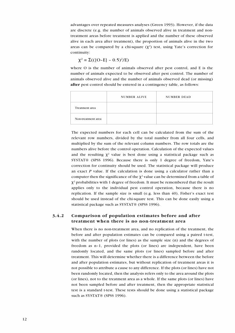
advantages over repeated measures analyses (Green 1993). However, if the data

are discrete (e.g. the number of animals observed alive in treatment and non-

treatment areas before treatment is applied and the number of these observed

alive in each area after treatment), the proportion of animals alive in the two

areas can be compared by a chi-square (χ2) test, using Yate�s correction for

continuity:

χ2 = Σ(([O�E] � 0.5)2/E)

where O is the number of animals observed after pest control, and E is the

number of animals expected to be observed after pest control. The number of

animals observed alive and the number of animals observed dead (or missing)

after pest control should be entered in a contingency table, as follows:

The expected numbers for each cell can be calculated from the sum of the

relevant row numbers, divided by the total number from all four cells, and

multiplied by the sum of the relevant column numbers. The row totals are the

numbers alive before the control operation. Calculation of the expected values

and the resulting χ2 value is best done using a statistical package such as

SYSTAT® (SPSS 1996). Because there is only 1 degree of freedom, Yate�s

correction for continuity should be used. The statistical package will produce

an exact P value. If the calculation is done using a calculator rather than a

computer then the significance of the χ2 value can be determined from a table of

χ2 probabilities with 1 degree of freedom. It must be remembered that the result

applies only to the individual pest control operation, because there is no

replication. If the sample size is small (e.g. less than 40), Fisher�s exact test

should be used instead of the chi-square test. This can be done easily using a

statistical package such as SYSTAT® (SPSS 1996).

3.4.2 Comparison of population estimates before and aftertreatment when there is no non-treatment area

When there is no non-treatment area, and no replication of the treatment, the

before and after population estimates can be compared using a paired t-test,

with the number of plots (or lines) as the sample size (n) and the degrees of

freedom as n�1, provided the plots (or lines) are independent, have been

randomly located, and the same plots (or lines) sampled before and after

treatment. This will determine whether there is a difference between the before

and after population estimates, but without replication of treatment areas it is

not possible to attribute a cause to any difference. If the plots (or lines) have not

been randomly located, then the analysis refers only to the area around the plots

(or lines), not to the treatment area as a whole. If the same plots (or lines) have

not been sampled before and after treatment, then the appropriate statistical

test is a standard t-test. These tests should be done using a statistical package

such as SYSTAT® (SPSS 1996).

NUMBER ALIVE NUMBER DEAD

Treatment area

Non-treatment area

13

If the data are not normally distributed or the variances are unequal, even after

transformation, then non-parametric methods of analysis may be used in place

of the t-tests (e.g. Kruskal-Wallis or Mann-Whitney tests). Again, these tests

should be done using a statistical package such as SYSTAT® (SPSS 1996).

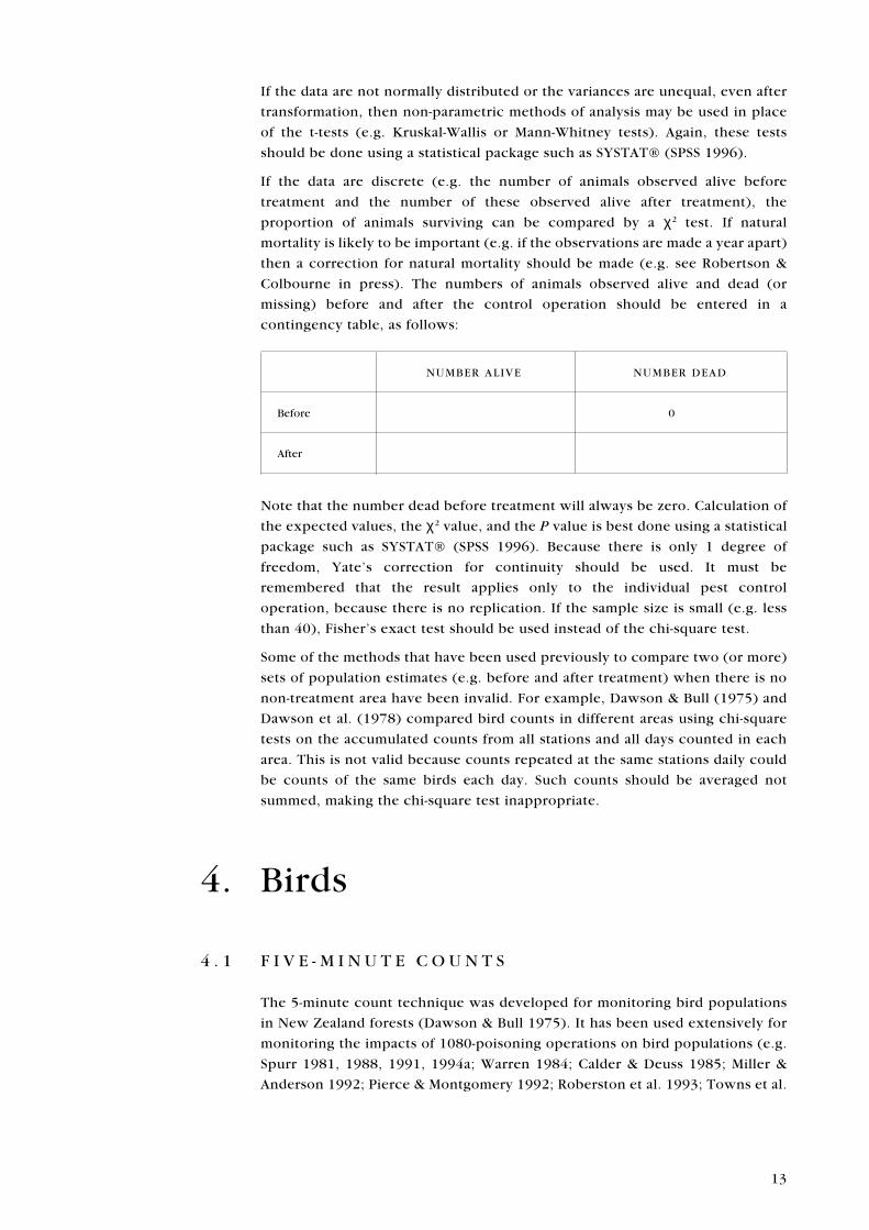
If the data are discrete (e.g. the number of animals observed alive before

treatment and the number of these observed alive after treatment), the

proportion of animals surviving can be compared by a χ2 test. If natural

mortality is likely to be important (e.g. if the observations are made a year apart)

then a correction for natural mortality should be made (e.g. see Robertson &

Colbourne in press). The numbers of animals observed alive and dead (or

missing) before and after the control operation should be entered in a

contingency table, as follows:

Note that the number dead before treatment will always be zero. Calculation of

the expected values, the χ2 value, and the P value is best done using a statistical

package such as SYSTAT® (SPSS 1996). Because there is only 1 degree of

freedom, Yate�s correction for continuity should be used. It must be

remembered that the result applies only to the individual pest control

operation, because there is no replication. If the sample size is small (e.g. less

than 40), Fisher�s exact test should be used instead of the chi-square test.

Some of the methods that have been used previously to compare two (or more)

sets of population estimates (e.g. before and after treatment) when there is no

non-treatment area have been invalid. For example, Dawson & Bull (1975) and

Dawson et al. (1978) compared bird counts in different areas using chi-square

tests on the accumulated counts from all stations and all days counted in each

area. This is not valid because counts repeated at the same stations daily could

be counts of the same birds each day. Such counts should be averaged not

summed, making the chi-square test inappropriate.

4. Birds

4 . 1 F I V E - M I N U T E C O U N T S

The 5-minute count technique was developed for monitoring bird populations

in New Zealand forests (Dawson & Bull 1975). It has been used extensively for

monitoring the impacts of 1080-poisoning operations on bird populations (e.g.

Spurr 1981, 1988, 1991, 1994a; Warren 1984; Calder & Deuss 1985; Miller &

Anderson 1992; Pierce & Montgomery 1992; Roberston et al. 1993; Towns et al.

NUMBER ALIVE NUMBER DEAD

Before 0

After

14

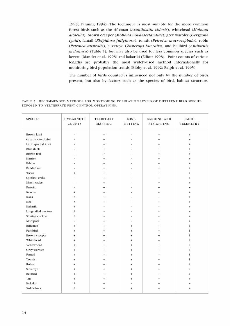
1993; Fanning 1994). The technique is most suitable for the more common

forest birds such as the rifleman (Acanthisitta chloris), whitehead (Mohoua

albicilla), brown creeper (Mohoua novaeseelandiae), grey warbler (Gerygone

igata), fantail (Rhipidura fuliginosa), tomtit (Petroica macrocephala), robin

(Petroica australis), silvereye (Zosterops lateralis), and bellbird (Anthornis

melanura) (Table 3), but may also be used for less common species such as

kereru (Mander et al. 1998) and kakariki (Elliott 1998). Point counts of various

lengths are probably the most widely-used method internationally for

monitoring bird population trends (Bibby et al. 1992; Ralph et al. 1995).

The number of birds counted is influenced not only by the number of birds

present, but also by factors such as the species of bird, habitat structure,

TABLE 3 . RECOMMENDED METHODS FOR MONITORING POPULATION LEVELS OF DIFFERENT BIRD SPECIES

EXPOSED TO VERTEBRATE PEST CONTROL OPERATIONS.

SPECIES FIVE -MINUTE TERRITORY MIST- BANDING AND RADIO-

COUNTS MAPPING NETTING RESIGHTING TELEMETRY

Brown kiwi � + � + +

Great spotted kiwi � + � + +

Little spotted kiwi � + � + +

Blue duck � + � + +

Brown teal � ? � + +

Harrier � + � + +

Falcon � + � + +

Banded rail � + � + +

Weka + + � + +

Spotless crake � + � + +

Marsh crake � + � + +

Pukeko � + � + +

Kereru + + � � +

Kaka ? + � � +

Kea ? + � + +

Kakariki + � � � +

Long-tailed cuckoo ? � � � +

Shining cuckoo ? � � � +

Morepork � + � � +

Rifleman + + + + ?

Fernbird + + + + ?

Brown creeper + + + + ?

Whitehead + + + + ?

Yellowhead + + + + ?

Grey warbler + + + + ?

Fantail + + + + ?

Tomtit + + + + ?

Robin + + + + ?

Silvereye + + + + ?

Bellbird + + + + ?

Tui + + + + +

Kokako ? + � + +

Saddleback ? + + + +

15

topography, weather, time of day, season, and ability of the observers. These

influences must be standardised or eliminated if valid indices of density are to

be made. The counts of different species are not comparable because each

species has a different detectability (e.g. the bellbird is more likely to be

detected than the rifleman because it has a more conspicuous call). Thus, each

species must be recorded and analysed separately. Treatment and non-

treatment areas should be similar in habitat and topography, and be counted on

the same days (using two observers, one in each area at the same time) and an

equal number of times by each observer (by observers swapping between areas

on different days). Only observers able to accurately identify birds from their

sounds (songs and calls) as well as by sight should participate in bird surveys. If

differences between observers are great, they could reduce the power of

monitoring to detect changes in bird populations. Observer differences may not

be important if the same observers count in both areas before and after

treatment. However, observer bias is important if different observers are used

from year to year in long-term studies. Observers also need to be trained to

estimate the distances to birds seen and/or heard (see below).

According to Dawson (1981), unless a bird species is very abundant (>1 per

count) and large numbers of counts are made (>30), the technique has low

power (i.e. can detect only large changes (>50%) in forest bird populations).

For example, 48 counts are needed to detect a 40% change, 85 counts to detect

a 30% change, 192 counts to detect a 20% change, and 770 counts to detect a

10% change in a species with an average of 1 bird per count.

We are aware of only one study that has attempted to relate the numbers

detected by the 5-minute count technique to known numbers of a species in

New Zealand. Gill (1980) found that 5-minute counts of grey warblers and

robins varied in proportion to their true densities. This correlation has not been

verified for other bird species. Cassey (1997) found that 5-minute point-distance

counts (i.e. 5-minute counts with distances to birds estimated) over-estimated

the true density of saddlebacks (Philesturnus carunculatus), but whether this

was a result of the 5-minute count itself or the distance extrapolations used to

convert the count to density is unclear.

Five-minute counts are not suitable for monitoring short-term impacts of pest

control on individual birds because individual territory-holders that die from

poisoning may be quickly replaced by �floating� non-territorial birds. This

replacement can only be detected by observations of individually marked (e.g.

banded) birds (see below). In addition, the new territory-holders may establish

their presence by calling and singing more frequently, making them more

detectable in 5-minute counts. Some birds may also become unpaired as a result

of pest control and, especially if males, may increase their rate of calling and

singing. For example, the death of several territorial blackbirds (Turdus

merula) as a result of an aerial 1080-poisoning operation in The Cone in

September 1977 caused increased singing by both the replacement birds and

the surrounding surviving birds, which caused an increase in the numbers

counted in 5-minute counts made 2 weeks after poisoning (E.B. Spurr unpubl.

data). Likewise, Empson & Miskelly (1999) found 5-minute counts of robins

increased as a result of increased vocalisation after an aerial brodifacoum-

poisoning operation on Kapiti Island in September�October 1996 although the

16

number of robins had decreased. Thus, 5-minute counts should not be done

until several weeks or months after pest control operations, to allow any

disruption to the behaviour of birds to stabilise.

4.1.1 Equipment

� map(s) � data recording cards

� notebook � hip-chain and cotton

� pen/pencil plus spare � compass

� plastic tape � spirit marker pen

� wristwatch (digital or with a second hand)

� binoculars (e.g. 8×30 or 7×50, suitable for use in dim forest light)

4.1.2 Method

Counting stations should be located randomly, stratified randomly, or

systematically on randomly located transect lines, in treatment and non-

treatment areas, if they are to represent the areas as a whole. If they are not

located randomly (e.g. located on a circuit) they will not represent the area as a

whole, only the circuit within the area. The stations should be at least 200 m

from the edge of the survey area, and a minimum of 200 m apart. At this

distance, there is little chance of counting the same bird at adjacent stations

(Bibby et al. 1992; Ralph et al. 1995), especially in the breeding season for small

forest passerines such as grey warblers, tomtits, and robins that have territories

or home ranges of less than about 4 ha (200 m × 200 m). For these species the

counting stations will be independent. However, the counting stations will not

be independent for larger species such as kaka (Nestor meridionalis) and

kereru (Hemiphaga novaeseelandiae) that have much larger territories or

home ranges. For these species, data could be analysed from every second

station (which would give a spacing of 400 m). In some previous studies,

counting stations have been only 100 m apart, but at this spacing they are

unlikely to be independent even for small forest passerines. When counting

stations are on transect lines, a hip-chain should be used to locate them exactly

200 m apart, to avoid bias in �selecting� the location. Counting stations and the

route between them should be clearly marked (e.g. with plastic tape) in both

directions so that they can be re-located. The hip-chain cotton must be removed

afterwards to prevent birds becoming tangled in it and dying.

For statistical purposes, the number of counting stations (or lines of counting

stations) should be as great as possible. From a practical point of view, the

maximum number of stations that can be counted by one observer in 1 day is

20�40, depending upon the terrain and the distance between stations (or lines).

If stations are located on transect lines, it is better to have 10 lines of four

stations, for example, than 4 lines of ten stations.

Each observer needs to make only one count at each counting station before

and after treatment. Repeat counts (e.g. two or more counts at the same

counting station) by the same observer will improve the accuracy of the data for

each counting station, and consequently for each area being surveyed.

However, for statistical reasons, it is better to increase the number of counting

stations than to repeat counts by the same observer at existing stations.

17

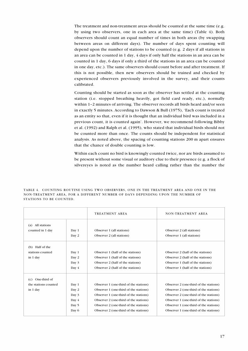
The treatment and non-treatment areas should be counted at the same time (e.g.

by using two observers, one in each area at the same time) (Table 4). Both

observers should count an equal number of times in both areas (by swapping

between areas on different days). The number of days spent counting will

depend upon the number of stations to be counted (e.g. 2 days if all stations in

an area can be counted in 1 day, 4 days if only half the stations in an area can be

counted in 1 day, 6 days if only a third of the stations in an area can be counted

in one day, etc.). The same observers should count before and after treatment. If

this is not possible, then new observers should be trained and checked by

experienced observers previously involved in the survey, and their counts

calibrated.

Counting should be started as soon as the observer has settled at the counting

station (i.e. stopped breathing heavily, got field card ready, etc.), normally

within 1�2 minutes of arriving. The observer records all birds heard and/or seen

in exactly 5 minutes. According to Dawson & Bull (1975), �Each count is treated

as an entity so that, even if it is thought that an individual bird was included in a

previous count, it is counted again�. However, we recommend following Bibby

et al. (1992) and Ralph et al. (1995), who stated that individual birds should not

be counted more than once. The counts should be independent for statistical

analysis. As noted above, the spacing of counting stations 200 m apart ensures

that the chance of double counting is low.

Within each count no bird is knowingly counted twice, nor are birds assumed to

be present without some visual or auditory clue to their presence (e.g. a flock of

silvereyes is noted as the number heard calling rather than the number the

TABLE 4 . COUNTING ROUTINE USING TWO OBSERVERS, ONE IN THE TREATMENT AREA AND ONE IN THE

NON-TREATMENT AREA, FOR A DIFFERENT NUMBER OF DAYS DEPENDING UPON THE NUMBER OF

STATIONS TO BE COUNTED.

TREATMENT AREA NON-TREATMENT AREA

(a) All stations

counted in 1 day Day 1 Observer 1 (all stations) Observer 2 (all stations)

Day 2 Observer 2 (all stations) Observer 1 (all stations)

(b) Half of the

stations counted Day 1 Observer 1 (half of the stations) Observer 2 (half of the stations)

in 1 day Day 2 Observer 1 (half of the stations) Observer 2 (half of the stations)

Day 3 Observer 2 (half of the stations) Observer 1 (half of the stations)

Day 4 Observer 2 (half of the stations) Observer 1 (half of the stations)

(c) One-third of

the stations counted Day 1 Observer 1 (one-third of the stations) Observer 2 (one-third of the stations)

in 1 day Day 2 Observer 1 (one-third of the stations) Observer 2 (one-third of the stations)

Day 3 Observer 1 (one-third of the stations) Observer 2 (one-third of the stations)




18

observer guesses such a frequency of calling would represent; if a bird calls in

one place and later one of the same species calls some distance away, they are

taken as two individuals unless there is evidence that the first bird moved to the

second place) (Dawson & Bull 1975).

Do not count birds judged to be more than 200 m away (Dawson & Bull 1975).

Ralph et al. (1995) recommended counting all birds detected (but not birds

already counted) to maximise the amount of data recorded, but we do not

recommend this. However, there is unlikely to be much difference between the

two methods because most birds are detected within 200 m. Both methods

excluded birds flying overhead and judged not to belong to the area being

surveyed.

Ramsey & Scott (1979, 1981) and Reynolds et al. (1980) recommended

recording the distances to birds that are detected and using these distances to

estimate the area surveyed (see also Bibby et al. 1992). This allows estimates of

species density to be made (Fancy 1997). Cassey (1997) used this technique to

estimate the density of saddlebacks in two habitats on Tiritiri Matangi Island.

However, the technique requires large sample sizes and relatively precise

estimates of distances, and for this it is necessary to use highly trained

observers. We are not in a position to recommend recording distances at

present. Recording distances to birds does not prevent analysis of the data as if

distances had not been recorded, for comparison with previous counts where

distances were not recorded.

Counts should be made within the period from about 1.5 hours after sunrise to

1.5 hours before sunset, to avoid the changes in bird conspicuousness near

dawn and dusk. In mid-winter, this means that counts should be made between

0930 and 1530 (NZ Standard Time). In mid-summer, the equivalent times are

0730 to 1930 (NZ Summer Time). Counts should be made throughout the day,

centred around the solar noon (1230), rather than be made all in the morning or

all in the afternoon. Counts should not be made during strong winds or heavy

rain, because these conditions affect the behaviour of birds and the ability of

observers to detect them.

The best time of year for making 5-minute counts is in the breeding season, in

spring and early summer (September�December), when birds are relatively

sedentary and dispersed on breeding territories. In the autumn and winter some

species, such as silvereyes, form large mobile flocks, which means that counts

of individuals will not be independent. Thus, for pest control operations in

winter, pre-poison surveys should be made in the previous spring�early

summer, and post-poison surveys in the following spring�early summer.

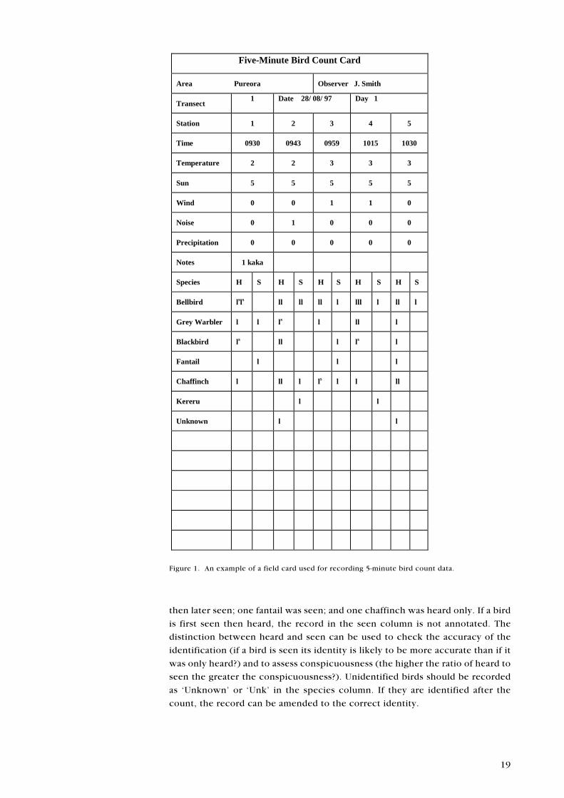
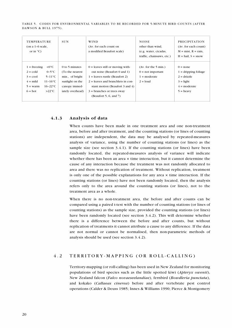
Counts are best recorded on specially prepared field cards (Fig. 1). The name of

the survey area, the name of the observer, the date (D/M/Y), day of survey (1, 2,

3, etc.), and transect number should be recorded once on each card. The

following information should be recorded for each count: station number, time

at start of count, and codes for temperature, sun, wind, noise, and precipitation

(see Table 5). Each bird observed should be recorded by a stroke in either the

heard or seen columns on the field card. If a bird is first heard and later seen, the

record in the heard column should be annotated with an �s�. Thus, in Fig. 1,

station 1, two bellbirds were first heard then later both seen; one grey warbler

was heard only and another seen (i.e. first seen); one blackbird was first heard

19

Figure 1. An example of a field card used for recording 5-minute bird count data.

then later seen; one fantail was seen; and one chaffinch was heard only. If a bird

is first seen then heard, the record in the seen column is not annotated. The

distinction between heard and seen can be used to check the accuracy of the

identification (if a bird is seen its identity is likely to be more accurate than if it

was only heard?) and to assess conspicuousness (the higher the ratio of heard to

seen the greater the conspicuousness?). Unidentified birds should be recorded

as �Unknown� or �Unk� in the species column. If they are identified after the

count, the record can be amended to the correct identity.

Five-Minute Bird Count Card

Area Pureora Observer J. Smith

Transect1 Date 28/ 08/ 97 Day 1

Station 1 2 3 4 5

Time 0930 0943 0959 1015 1030

Temperature 2 2 3 3 3

Sun 5 5 5 5 5

Wind 0 0 1 1 0

Noise 0 1 0 0 0

Precipitation 0 0 0 0 0

Notes 1 kaka

Species H S H S H S H S H S

Bellbird lsls ll ll ll l lll l ll l

Grey Warbler l l ls l ll l

Blackbird ls ll l ls l

Fantail l l l

Chaffinch l ll l ls l l ll

Kereru l l

Unknown l l

20

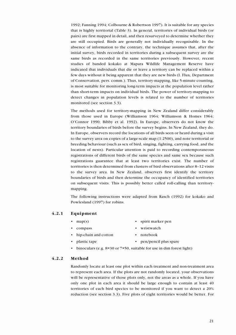
4.1.3 Analysis of data

When counts have been made in one treatment area and one non-treatment

area, before and after treatment, and the counting stations (or lines of counting

stations) are independent, the data may be analysed by repeated-measures

analysis of variance, using the number of counting stations (or lines) as the

sample size (see section 3.4.1). If the counting stations (or lines) have been

randomly located, the repeated-measures analysis of variance will indicate

whether there has been an area × time interaction, but it cannot determine the

cause of any interaction because the treatment was not randomly allocated to

area and there was no replication of treatment. Without replication, treatment

is only one of the possible explanations for any area × time interaction. If the

counting stations (or lines) have not been randomly located, then the analysis

refers only to the area around the counting stations (or lines), not to the

treatment area as a whole.

When there is no non-treatment area, the before and after counts can be

compared using a paired t-test with the number of counting stations (or lines of

counting stations) as the sample size, provided the counting stations (or lines)

have been randomly located (see section 3.4.2). This will determine whether

there is a difference between the before and after counts, but without

replication of treatments it cannot attribute a cause to any difference. If the data

are not normal or cannot be normalised, then non-parametric methods of

analysis should be used (see section 3.4.2).

4 . 2 T E R R I T O R Y - M A P P I N G ( O R R O L L - C A L L I N G )

Territory-mapping (or roll-calling) has been used in New Zealand for monitoring

populations of bird species such as the little spotted kiwi (Apteryx owenii),

New Zealand falcon (Falco novaeseelandiae), fernbird (Bowdleria punctata),

and kokako (Callaeas cinerea) before and after vertebrate pest control

operations (Calder & Deuss 1985; Innes & Williams 1990; Pierce & Montgomery

TABLE 5 . CODES FOR ENVIRONMENTAL VARIABLES TO BE RECORDED FOR 5 -MINUTE BIRD COUNTS (AFTER

DAWSON & BULL 1975) .

TEMPERATURE SUN WIND NOISE PRECIPITATION

(on a 1�6 scale, (Av. for each count on other than wind, (Av. for each count)

or in °C) a modified Beaufort scale) (e.g. water, cicadas, M = mist, R = rain,

traffic, chainsaws, etc.) H = hail, S = snow

1 = freezing <0°C 0 to 5 minutes 0 = leaves still or moving with- (Av. for the 5 min.) 0 = none

2 = cold 0�5°C (To the nearest out noise (Beaufort 0 and 1) 0 = not important 1 = dripping foliage

3 = cool 5�11°C min., of bright 1 = leaves rustle (Beaufort 2) 1 = moderate 2 = drizzle

4 = mild 11�16°C sunlight on the 2 = leaves and branchlets in con- 2 = loud 3 = light

5 = warm 16�22°C canopy immed- stant motion (Beaufort 3 and 4) 4 = moderate

6 = hot >22°C iately overhead) 3 = branches or trees sway 5 = heavy

(Beaufort 5, 6, and 7)

21

1992; Fanning 1994; Colbourne & Robertson 1997). It is suitable for any species

that is highly territorial (Table 3). In general, territories of individual birds (or

pairs) are first mapped in detail, and then resurveyed to determine whether they

are still occupied. Birds are generally not individually recognisable. In the

absence of information to the contrary, the technique assumes that, after the

initial survey, birds recorded in territories during a subsequent survey are the

same birds as recorded in the same territories previously. However, recent

studies of banded kokako at Mapara Wildlife Management Reserve have

indicated that individuals that die or leave a territory can be replaced within a

few days without it being apparent that they are new birds (I. Flux, Department

of Conservation, pers. comm.). Thus, territory-mapping, like 5-minute counting,

is most suitable for monitoring long-term impacts at the population level rather

than short-term impacts on individual birds. The power of territory-mapping to

detect changes in population levels is related to the number of territories

monitored (see section 3.3).

The methods used for territory-mapping in New Zealand differ considerably

from those used in Europe (Williamson 1964; Williamson & Homes 1964;

O�Connor 1990; Bibby et al. 1992). In Europe, observers do not know the

territory boundaries of birds before the survey begins. In New Zealand, they do.

In Europe, observers record the locations of all birds seen or heard during a visit

to the survey area on copies of a large-scale map (1:2500), and note territorial or

breeding behaviour (such as sex of bird, singing, fighting, carrying food, and the

location of nests). Particular attention is paid to recording contemporaneous

registrations of different birds of the same species and same sex because such

registrations guarantee that at least two territories exist. The number of

territories is then determined from clusters of bird observations after 8�12 visits

to the survey area. In New Zealand, observers first identify the territory

boundaries of birds and then determine the occupancy of identified territories

on subsequent visits. This is possibly better called roll-calling than territory-

mapping.

The following instructions were adapted from Rasch (1992) for kokako and

Powlesland (1997) for robins.

4.2.1 Equipment

� map(s) � spirit marker pen

� compass � wristwatch

� hip-chain and cotton � notebook

� plastic tape � pen/pencil plus spare


4.2.2 Method

Randomly locate at least one plot within each treatment and non-treatment area

to represent each area. If the plots are not randomly located, your observations

will be representative of those plots only, not the areas as a whole. If you have

only one plot in each area it should be large enough to contain at least 40

territories of each bird species to be monitored if you want to detect a 20%

reduction (see section 3.3). Five plots of eight territories would be better. For

22

small birds (e.g. robins and tomtits) with territories of 2.5 ha, plots need to be at

least 100 ha to contain 40 territories. To contain eight territories, plots should

be at least 20 ha. For small birds in forest, grid each plot with taped lines at 100-

m intervals, with each line being numbered at 50-m intervals so that observers

can determine where they are when they hear or see a bird. For large birds (e.g.

kaka, New Zealand falcons, and kokako), which have larger territories, the

survey area needs to be much larger and plots do not need to be gridded. Draw

large-scale maps of each survey area on which to record the locations of the bird

territories.

Determine the boundaries of all bird territories by making repeat visits to each

plot, mapping the location of all birds encountered and paying particular

attention to simultaneous observations of different birds of the same species

and sex because such observations indicate different territories. If possible,

follow birds to obtain a clear picture of the extent of their territory. For kokako,

it is recommended that routes taken by birds be recorded on a map or �follow

sheet� (Rasch 1992). All neighbouring birds should be clearly identified. More

than one person is usually necessary to identify neighbours, the number of

people depending upon the number of birds with adjacent territories. Initial

determination of territory boundaries may take some time. For kokako, it may

take as many as 12 visits per territory, or 5 person-weeks per territory, to map

the territories in a dense population (Rasch 1992).

Decide what constitutes a survey for resighting (roll-calling) birds in your study.

It may mean a single half-hour search of each identified territory, or it may mean

an initial half- hour search of each territory and then going back to locate any

known territorial birds that were missed on the initial search. Decide whether

the survey must be completed within 1 day, 2 days, or 1 week. Whatever you

decide must be adhered to for all surveys, before and after the control

operation. For kokako, it may take from less than 1 hour to more than 4 hours to

re-locate an individual on its territory (Rasch 1992).

On each survey, keep a record of the presence and absence of birds seen in each

territory. Be specific about what you record. For example; �heard bird calling in

territory A but not seen�, �saw bird in territory A but unable to determine sex�,

or �saw male in territory A�. If any birds are banded indicate this: e.g. �saw

banded bird in territory A but unable to determine sex or identity�, or �saw male

M-Y/R in territory A�.

If the control operation is in spring or early summer, surveys should be repeated

weekly for at least 4 weeks before the expected date of the control operation.

Continue the weekly monitoring if the operation is delayed. After the control

operation, monitor the presence/absence of birds in each known territory

weekly for at least 4 weeks for 1080-poisoning operations and for at least 10

weeks for brodifacoum-poisoning operations, starting 1 week after poisoning. If

the control operation is in autumn or winter, then for seasonally territorial

species territory-mapping and roll-calling must be done in the spring before and

after the operation because the method is restricted to the breeding season. For

species that are territorial throughout the year, such as kokako, territory-

mapping and roll-calling can be done at any time of the year. Only birds located

on their territories at least once a week for 4 weeks before pest control should

be included in the data analysis.

23


The number of occupied territories in the treatment and non-treatment areas

before and after pest control should be compared using the chi-square test or

Fisher�s exact test, to determine whether there is a significant difference in the

survival of birds in the two areas (see section 3.4.1). If there is no non-treatment

area, the chi-square test or Fisher�s exact test can be used to compare the

number of occupied territories in the treatment area before and after pest

control (see section 3.4.2).

4 . 3 M I S T - N E T T I N G C A P T U R E R A T E S

The capture rates of birds caught in mist nets have been used as indices for

monitoring bird population trends overseas (Karr 1981; Ralph et al. 1993) and

for comparing bird abundance in different forest types in New Zealand (Spurr et

al. 1992), but have not yet been used for monitoring the impacts of vertebrate

pest control on bird population trends. The method is most suitable for small

passerines such as riflemen, whiteheads, brown creepers, grey warblers,

fantails, tomtits, robins, silvereyes, and bellbirds that are relatively sedentary

and have small home ranges (see Table 3). If standard mist nets are used the

sampling will be restricted to birds flying below about 3 m. However, if

necessary, nets can be raised into the forest canopy to sample birds there (Spurr

et al. 1992; Dilks et al. 1995). The method can be used only by people

experienced with using mist nets.

In addition to capture rates, survival rates of birds can be calculated (from

recaptures) because birds that are captured are banded with numbered metal

leg-bands. Thus, mist-netting, unlike 5-minute counting and territory-mapping,

is potentially suitable for monitoring both short-term impacts on individual

birds and long-term impacts on bird populations. The power of mist-netting to

detect changes in bird population trends has not been determined.

4.3.1 Equipment

� banding permit � banding pliers

� mist nets � cloth bags for holding birds

� poles for mist nets � scales

� bands � notebook

� pen or pencil plus spare

Handling and banding permits, appropriate-sized metal bands, banding pliers,

and mist nets can be obtained from the Banding Office, Department of

Conservation, PO Box, 10420, Wellington. Animal Ethics Committee approval

will also need to be obtained. Ensure all mist nets are the same size and have an

appropriate mesh size for the target species. Poles for mist nets should be made

from aluminium tubing (obtainable from hardware suppliers). For convenience,

make the poles telescopic by using two sizes of aluminium tubing, so that one

fits snugly inside the other (Dilks et al. 1995).

24

4.3.2 Method

Randomly locate at least five transects in both the treatment and non-treatment

areas if you wish these transects to represent each area. If the transects are not

randomly located, data collected from them will be representative of those

transects only, not the areas as whole. The transects within each area should be

far enough apart so that the same birds are not caught on different transects (i.e.

at least 500 m apart). On each transect, erect three to five mist nets at sites where

the vegetation is amenable to mist-netting. Some clearance of vegetation may be

necessary to prevent snagging and tearing the mist nets. The mist nets can be in a

line end to end or spaced further apart. Permanently mark the mist-net sites so

that they can be relocated after pest control. Lures (e.g. tape recordings of bird

calls) must not be used to attract birds to mist nets because capture rates should

represent unmodified rates of net interception (Karr 1981).

All transects within an area do not have to be sampled on the same days, but the

same number of transects should be sampled on the same days and at the same

times of day in both treatment and non-treatment areas. Mist nets should be

operated throughout the day, from about 0800 to 1800 hours, though capture

rates are usually highest in the early morning and evening. Mist-netting should be

done for no more than 2 days at each net site (otherwise birds may avoid

recapture) then the nets shifted to a new site if necessary. Aim for 100 mist-net

hours per transect. Mist-netting should be restricted to fine days or days with light

rain only and checked every 15 to 30 minutes to minimise bird mortality. All birds

captured should be banded with numbered metal leg-bands to enable recaptures

to be identified. The data can be separated into first captures and recaptures.

The best time of year for obtaining mist-net capture rates is in the breeding

season, in spring and early summer (September�December), when birds are

relatively sedentary and dispersed on breeding territories. At this time of year,

Spurr et al. (1992) caught about one bird of each of the more common small

passerines per 100 mist-net hours in lowland podocarp forest. Thus, for pest

control operations in winter, pre-poison surveys should be made in the previous

spring�early summer, and post-poison surveys in the following spring�early

summer. Mist-netting in autumn, after the breeding season, provides data on the

relative abundance of young and adult birds.


If there are treatment and non-treatment areas, the data (birds, by species, per

100 mist-net hours) should be analysed by repeated measures analysis of

variance, to determine whether there has been an area × time interaction (see

section 3.4.1). If there are no non-treatment areas, the capture rates before and

after pest control can be compared using a paired t-test (see section 3.4.2). If

the data are not normal or cannot be normalised, then non-parametric methods

of analysis should be used (see section 3.4.2).

4 . 4 B A N D I N G A N D R E C A P T U R I N G O R R E S I G H T I N G

Birds have been captured and banded with numbered metal bands and/or

unique combinations of coloured plastic bands, and then recaptured or

resighted several times before and after vertebrate pest control operations to

25

determine the impacts on individual birds of species such as fernbirds, tomtits,

robins, and kokako (e.g. Pierce & Montgomery 1992; Ranum et al. 1994; Walker

1997a; Powlesland et al. 1998, 1999). This technique is suitable for any species

that can be recaptured or resighted relatively frequently (see Table 3). It

assumes that birds that disappear have died as a result of pest control (e.g. 1080-

poisoning). Few dead banded birds have been found after pest control

operations, but a large proportion of those that have been found have contained

residues of poison. The technique can also provide information on the impacts

of pest control on bird populations, but it requires more effort than with 5-

minute counts. Only one or a few species can be monitored at a time. The

method can be combined with territory-mapping. Banding birds is not restricted

to the breeding season as is territory-mapping, but it may be easier in the

breeding season because birds are more sedentary then and therefore are likely

to be resighted more readily. The power of banding studies to detect changes in

bird population levels is related to the number of birds banded (see section 3.3).

The following instructions were adapted from Powlesland (1997).

4.4.1 Equipment

� banding permit � bands

� mist nets � banding pliers

� poles for mist nets � cloth bags for holding birds

� cassette tape recorder � scales

� tape of bird calls � notebook

� pen or pencil plus spare


Handling and banding permits, appropriate-sized metal and colour bands,

banding pliers, and mist nets can be obtained from the Banding Office,

Department of Conservation, PO Box, 10420, Wellington. Animal Ethics

Committee approval will also need to be obtained. Poles for mist nets should be

aluminium tubing (obtainable from hardware suppliers). Use two sizes so that

one will fit snugly inside the other to make the poles telescopic (Dilks et al.

1995). Obtain a portable cassette tape recorder, tapes, and taped calls of birds

from Cognita (formerly Conservation Design Centre), Nelson, or preferably by

taping calls in your study area. For robins, obtain a clap-trap and/or a hand-net,

and a supply of mealworms or other readily available invertebrate food that the

birds will eat.

4.4.2 Method

Randomly locate at least one plot within each treatment and non-treatment area

(as for territory mapping). If you have only one plot it should be large enough to

contain at least 40 birds of each species to be monitored. Five plots of eight

birds would be better statistically but more difficult operationally. For small

birds (such as robins and tomtits), plots need to be at least 100 ha to contain 40

birds. To contain eight birds, plots should be at least 20 ha. Grid each plot with

taped lines at about 100-m intervals, with each line being numbered at 50-m

intervals so that observers can determine where they are when they hear or see

a bird. This will aid with re-locating birds. For large birds such as kaka, New

Zealand falcons, and kokako, the survey area needs to be much larger than for

26

small birds, but will not need to be marked so intensively. Draw large-scale

maps of each survey area on which to record the locations of the birds.

Erect mist nets or set up other capturing devices, such as clap-traps for robins,

at strategically located sites, where the vegetation is amenable to mist-netting,

within the randomly located plots. Capture and colour-band at least 30 birds in

each area, so that at least 75% of the birds are banded before monitoring starts.

Decide what constitutes a survey for resighting birds in your study. It may mean

a single day spent searching in each area, or it may mean an initial 1-day search

and then going back for a second day (or longer) to locate any known banded

birds missed on the initial search. Decide whether the survey must be

completed within 1 day, 2 days, or more. Whatever you decide must be adhered

to for all surveys, before and after the control operation.

On each survey, keep a record of the presence and absence of banded and

unbanded birds seen in each area. Be specific about what you record. For

example: �heard bird in territory A but not seen�, �saw bird in territory A but

unable to determine whether banded�, �saw banded bird in territory A but

unable to determine identity�, or �saw M-Y/R in territory A�. Repeat surveys

weekly for at least 4 weeks before the expected date of the control operation.

Continue the weekly monitoring if the operation is delayed. After the control

operation, monitor the presence/absence of banded birds weekly for at least 4

weeks for 1080-poisoning operations and for at least 10 weeks for brodifacoum-

poisoning operations, starting 1 week after poisoning.

The effect of poisoning on the bird population can then be assessed from the

minimum number of birds known to be alive (MNA) before pest control and the

minimum number known to be alive at various time-intervals after pest control.

The minimum number alive can be estimated by adding the number of

individuals recorded in the survey under consideration and the number of

banded individuals recorded in subsequent surveys but not during the survey

under consideration. A disadvantage of this method is that estimates after pest

control are based on fewer samples than estimates before pest control unless

data from the last survey are excluded from calculation of the minimum number

alive before pest control. If this is not done, the number alive after pest control

may be underestimated.


The number of banded birds in the treatment and non-treatment areas before and

after pest control should be compared using the chi-square test or Fisher�s exact

test, to determine whether there is a significant difference in the survival of birds

in the two areas (see section 3.4.1). If there is no non-treatment area, the chi-

square test or Fisher�s exact test can be used to compare the number of banded

birds in the treatment area before and after pest control (see section 3.4.2).

4 . 5 R A D I O - T E L E M E T R Y

Radio-telemetry has been used to monitor the impacts of vertebrate pest control

on some species of large birds, such as kiwi (Apteryx spp.), kaka, weka

(Gallirallus australis), morepork (Ninox novaeseelandiae), and blue duck

27

(Hymenolaimus malacorhynchos) (Pierce & Montgomery 1992; Robertson et

al. 1993; Greene 1995; Walker 1997a; Powlesland et al. 1998; Robertson et al.

1999a,b; Stephenson et al. 1999; Robertson & Colbourne in press). Radio-

transmitters have also been used to monitor survival of kereru, though not in

relation to vertebrate pest control (Clout et al. 1995; Pierce & Graham 1995),

and could be used for other species (see Table 3). Radio-transmitters (with or

without mortality sensors) enable individual birds to be located even after

death. The power of radio-telemetry studies to detect changes in bird survival is

related to the number of birds fitted with radio-transmitters (see section 3.3).

4.5.1 Equipment

� permits � bands

� mist nets � banding pliers

� poles for mist nets � radio-transmitters

� cassette tape recorder � harness for radio-transmitters

� tape of bird calls � radio-receiver

� cloth bags for holding birds � Yagi aerial

� scales


Obtain permits for capturing and handling birds, and for attaching radio-

transmitters to them, from the Department of Conservation, PO Box, 10420,

Wellington. Animal Ethics Committee approval will also need to be obtained.

Radio-tagged birds should also be banded, so obtain permits and equipment as

for banding birds (section 4.3.1).

Obtain mist nets, bands, and banding pliers (as in section 4.3.1). Obtain radio-

transmitters (preferably with mortality sensors), radio-receiver, and Yagi aerial

(e.g. from Sirtrack Ltd, PB 1403, Havelock North). Ensure that the weight of the

transmitter package (including battery) does not exceed 5% of the body weight

of the bird.

4.5.2 Method

Erect mist nets (see Dilks et al. 1995) or set up other capturing devices such as

clap-traps in treatment and non-treatment areas. Capture and attach radio-

transmitters to at least 40 birds in each area if you want the ability to detect a

20% reduction in numbers (see section 3.3).

Use a radio-receiver and Yagi aerial to locate individual birds (alive or dead)

daily for at least 4 days or once weekly for at least 4 weeks before pest control.

If the control operation is delayed, locate birds at least weekly until the

operation occurs. Relocate birds weekly for at least 4 weeks after 1080-

poisoning operations and for 10 weeks after brodifacoum-poisoning operations.


A chi-square test or Fisher�s exact test can be used to determine whether there

is a significant difference in survival of birds in the treatment and non-treatment

areas (see section 3.4.1).

28

4 . 6 O T H E R T E C H N I Q U E S

Various other techniques have been used to monitor populations of birds in spe-

cific situations: e.g. 1-hour or 2-hour night-time counts for kiwi (Robertson et al.

1993; Empson & Miskelly 1999; Robertson & Colbourne in press), display flight

monitoring and census counts from vantage points for kereru (Mander et al.

1998), and transect counts for kokako (Hudson & King 1993). Techniques for

monitoring birds of open country have not been specifically considered in this

manual. Techniques for monitoring waterfowl populations have also not been

considered in this manual. The choice of technique is influenced by individual

preference, resources available, and suitability of the technique for the species

(see Table 3).

5. Bats

Both short-tailed bats (Mystacina tuberculata) and long-tailed bats

(Chalinolobus tuberculatus) live in areas where vertebrate pest control

operations have been carried out, but there are no standard techniques for

monitoring their populations. There have been only two assessments of the

impacts of vertebrate pest control on bat populations: viz. the impacts of 1080-

poisoning on the short-tailed bat population in Rangataua Forest in August 1997

(Lloyd & McQueen 1998) and the impacts of brodifacoum-poisoning for the

eradication of rats on the short-tailed bat population on Codfish Island in August

1998 (P. McClelland, Department of Conservation, pers. comm.). Techniques

that have been used to monitor bat populations include counts of bats leaving

and/or entering daytime roosts, counts of echo-locations (�bat passes�) using

automatic bat detectors, and radio-telemetry of individual bats before and after

treatment. The Bat Recovery Plan (Molloy 1995) lists the development of survey

and monitoring techniques for bats as a top priority. The following instructions

are adapted from C.F.J. O�Donnell and P. McClelland (Department of

Conservation pers. comm.).

5 . 1 C O U N T S O F B A T S L E A V I N G A N D / O R E N T E R I N G

D A Y T I M E R O O S T S

Counts of bats leaving and/or entering daytime roosts have been used to

monitor short-tailed bat populations before and after 1080-poisoning for

possum control in Rangataua Forest in August 1997 (Lloyd & McQueen 1998)

and brodifacoum-poisoning for eradication of rodents on Codfish Island in

August 1998 (P. McClelland, Department of Conservation pers. comm.). The

exact methods have not yet been published.

29

5.1.1 Equipment

� video camera � monitor

� time-lapse video recorder � infrared light source

� video tapes � battery

5.1.2 Method

The exact methods have not yet been published. Video recorders are set up at

known roost sites. Video tapes are viewed and the total number of bats leaving

and/or entering the roosts counted.


No information obtained.

5 . 2 C O U N T S O F � B A T P A S S E S � R E C O R D E D B Y B A T

D E T E C T O R S

Bats emit ultrasonic sounds as they navigate, and these sounds are converted to

audible clicks as bats pass by an electronic bat detector. Bat detectors have been

used to determine the presence or absence of bats and could be used for

monitoring population abundance once standard procedures have been

developed (C.F.J. O�Donnell, Department of Conservation pers. comm.).

O�Donnell & Sedgeley (1994) developed an automatic monitoring system that

enables sampling the frequency of occurrence of bat calls all night, for several

nights if necessary. When short-tailed bats fly within c. 22 m of the detector, or

long-tailed bats within 50 m, the echo-location calls of the bats activate the

recorder and the sounds are recorded on tape. A talking clock speaks the time

every hour and is also recorded on tape.

The number of �bat passes� per hour provides an index of bat activity (rather

than the absolute number of bats). There is currently no information on how

the number of �bat passes� relates to the number of individual bats. A series of

passes in an hour could equally be produced by one bat passing several times or

several bats passing once. Bat activity is influenced by a number of factors,

including temperature and abundance of flying invertebrates. These factors

must be standardised or eliminated if valid indices of bat abundance are to be

made.

5.2.1 Equipment

� Batbox III bat detectors (Stag Electronics, Sussex, UK)

� voice-activated tape recorder

� talking clock

� battery (e.g. alkaline 9V, or sealed gel 12 V with voltage regulator)

� waterproof container to hold the above (see O�Donnell & Sedgeley 1994)

� thermometer (mercury maximum/minimum)

30

5.2.2 Method

Automatic monitoring systems should be located at randomly selected points in

treatment and non-treatment areas. The number and spacing of points have yet

to be decided. Four bat detectors at least 500 m apart were used on Codfish

Island (P. McClelland, Department of Conservation pers. comm.). The detectors

should be set at 27�28 kHz for short-tailed bats (Parsons 1997) and 40 kHz for

long-tailed bats (Parsons et al. 1997). The system should be left at the sample

point all night. The number of nights of sampling has yet to be decided. Surveys

should be made in summer when the weather is fine (clear, partly cloudy, or

overcast, but no rain or strong winds) and the temperature is >7°C.

The presence and absence of �bat passes� and �bat pass� rate per hour should be

tabulated after listening to the tapes. A �bat pass� is defined as a sequence of

greater than two echo-location calls as a bat flies past the microphone

(Furlonger et al. 1987). A sequence of audible clicks followed by a pause

delineates each �bat pass�. A full description of the method is given by

O�Donnell & Sedgeley (1994).



5 . 3 R A D I O - T E L E M E T R Y

Radio-transmitters can be successfully attached to bats, and daytime roosts

checked for the presence of radio-tagged bats before and after vertebrate pest

control operations. The power of radio-telemetry studies to detect changes in

bat survival is related to the number of bats fitted with radio-transmitters (see

section 3.3).

5.3.1 Equipment

� permits (handling, banding, Animal Ethics Committee)

� maps � radio-transmitters

� mist nets � radio-receiver

� harp traps � aerial

� cloth bags for holding bats � scales

5.3.2 Method




31

6. Reptiles

Several species of lizards (skinks and geckos) live in areas where 1080-poisoning

for possum control has been carried out, but the impact of poisoning on their

populations has never been monitored. Lizards and tuatara (Sphenodon

punctatus) also live on islands where brodifacoum-poisoning has been used for

rodent eradication, and a variety of methods has been used there to monitor

their population recovery.

Some population monitoring methods previously used, such as catch per unit

effort (CPUE), based on area searching, are not recommended because they are

inefficient, biased, and destroy lizard habitat (Towns 1991; Whitaker 1994). An

appropriate population monitoring technique for lizards has not been published

but the following instructions are adapted from Towns (1975, 1991, 1994),

Whitaker (1994), and Towns & Elliott (1996).

6 . 1 P I T F A L L T R A P P I N G

Pitfall trapping has been used to estimate the relative abundance of lizards

before and after brodifacoum-poisoning for rodents and on different islands

(Towns 1991, 1994). The number of lizards caught in pitfall traps is influenced

by population size as well as by a number of other factors (e.g. lizard species,

sex, and activity). However, when pitfall traps are used in paired treatment and

non-treatment areas, before and after application of a treatment, and analyses

are restricted to within species, factors apart from population size cancel out

unless there is an interaction between a factor such as lizard activity and

treatment (see also section 4.1). The power of pitfall trapping to detect changes

in population indices of lizards has not been determined.

6.1.1 Equipment

� maps � pitfall traps (see below)

� calipers or ruler � field cards or notebook

� cloth bag (for holding lizards) � pen or pencil

� spring balance (e.g. PesolaTM accurate to 0.1 g)

Pitfall traps should be made from 4-litre paint tins with the interior lacquered to

reduce rusting. The traps must have holes drilled in the bottom to drain water

away and avoid drowning captured lizards. The traps must also have a lid

supported 10�20 mm above them to protect captured lizards from the sun.

Animal Ethics Committee approval will be needed to capture reptiles.

6.1.2 Method

Pitfall traps should be located at 20 m intervals on randomly located transect

lines 100 m long (i.e. five traps per line). There should be at least five lines of

pitfall traps per survey area. Alternatively, clusters of five pitfall traps 2 m apart

may be located at five random points at least 20 m apart in the survey area.

32

The traps should be buried in the ground, with the rim flush or slightly below

the ground surface, and substrate packed close around the rim. When the traps

are set, the lids should be supported 10�20 mm above the rim of the traps.

When the traps are closed, a stout stick just longer than the diagonal height of

the trap should be placed inside each trap (Whitaker 1994). Do not use the lid to

close the trap because it could get dislodged.

The bait that should be used in the traps depends upon the target species. The

best baits are canned pears or canned fish-based cat-food (Whitaker 1994).

The traps should be checked daily for at least 4 days before and 4 days after a

pest control operation. For 1080-poisoning operations, the post-treatment

survey should be done at least 1 week after poisoning, and for brodifacoum-

poisoning operations, at least 2 weeks after poisoning. If the objective is to

determine if there are any long-term benefits of pest control, then annual

monitoring at the same time of year will be necessary because most New

Zealand lizards have low productivity.

Captured lizards should be identified to species and sex, and released alive

beside the trap where they were caught. The average capture rate per night

should be calculated for each trap, and the results expressed as the number of

lizards caught per 100 trap nights per transect line. If non-treatment areas are

surveyed, they should be surveyed on the same nights as the treatment areas (to

standardise seasonal and weather variables).


If there are treatment and non-treatment areas, the data (lizards per 100 trap-

nights) should be analysed by repeated measures analysis of variance, to

determine whether there has been an area × time interaction (see section

3.4.1). If there are no non-treatment areas, the capture rates before and after

pest control can be compared by a paired t-test (see section 3.4.2). If the data

are not normal or cannot be normalised, then non-parametric methods of

analysis should be used (see section 3.4.2).

6 . 2 M I N I M U M N U M B E R A L I V E

If captured lizards are individually marked then recaptures can be used to

estimate the minimum number alive (MNA) at different time points before and

after pest control (see Towns 1991, 1994; Patterson 1992; Towns & Elliott

1996). The assumptions of a closed population are accepted: viz., that there is

no large-scale movement of lizards into or out of the study areas between

sampling, and that there are few deaths of lizards eligible to be caught but not

caught (Towns 1994; Towns & Elliott 1996). The power of this technique to

detect changes in lizard population levels is related to the number of lizards

marked (see section 3.3).

6.2.1 Equipment

� maps � pitfall traps (as above)

� scissors (sharp) � calipers or ruler

33

� cloth bag (for holding lizards in) � field cards or notebook

� predetermined toe-clip combinations � pen or pencil

� spring balance (e.g. PesolaTM accurate to 0.1 g)

For predetermining toe-clip combinations, there are 150 individual

combinations from clipping two toes and 625 from clipping three toes

(Whitaker 1994). Animal Ethics Committee approval will need to be obtained to

capture and toe-clip reptiles.

6.2.2 Method

Lizards should be captured by pitfall trapping (as above) for 4 nights before and

at least two lots of 4 nights after pest control. Captured lizards should be

identified to species and sex, weighed to the nearest 0.1 g, measured in

millimetres from snout to vent, individually marked, and then released beside

the trap. See Whitaker (1994) for methods of identifying sex. The only

permanent method of marking is toe-clipping (Whitaker 1994). Remove toe(s)

quickly and cleanly with a sharp pair of scissors. Temporary methods of marking

include waterproof spirit-based felt pens, nail varnish, typists correction fluid,

and acrylic paint.

The minimum number alive before pest control can be estimated by adding the

following:

� The number of individuals caught on night 4 before pest control

� The number of previously marked individuals caught in subsequent trapping

sessions after pest control but not on night 4 before pest control

� The number of unmarked individuals caught in subsequent trapping sessions

after pest control but which were of sufficient snout�vent length (SVL) to sug-

gest that they had been alive but not caught on night 4 before pest control.

The minimum number alive after pest control can be estimated by adding the

following:

� The number of individuals marked before pest control that were caught in the

4 nights after pest control

� The number of unmarked individuals caught in the 4 nights after pest control

but which were of sufficient size (SVL) to suggest that they had been alive but

not caught before pest control

� The number of previously marked individuals caught in the second 4-night

trapping session after pest control but not in the first 4 nights after pest con-

trol

� The number of unmarked individuals caught in the second 4-night trapping

session after pest control but which were of sufficient size (SVL) to suggest

that they had been alive but not caught before pest control.

A disadvantage of this method is that estimates after pest control are based on

fewer samples than estimates before pest control unless data from the last 4-

night trapping session are excluded from calculation of the minimum number

alive before pest control. If this is not done, the number alive after pest control

may be underestimated.

34


The minimum number of lizards alive in the treatment and non-treatment areas

before and after pest control should be compared using the chi-square test or

Fisher�s exact test (see section 3.4.1). If there are no non-treatment areas, the

chi-square test or Fisher�s exact test should be used to compare the minimum

number of lizards alive before and after pest control (see section 3.4.2).


Other techniques are required for lizards that are not easy to trap (e.g. the grand

skink, Oligosoma grande, and the Otago skink, O. otagense), and for arboreal

species (e.g. the forest gecko, Hoplodactylus granulatus, and the common

green gecko, Naultinus elegans). Patterson (1992) suggested marking lizards

with acrylic paint without capturing them, by using a long stick, and then using

a mark-resighting technique to estimate abundance.

For tuatara, Cree et al. (1995) used the number of tuatara captured per person

per hour searched as a measure of abundance. Searches were made at night

using spotlights. Tuatara that were found were captured by hand and given a

unique toe-clip so that no tuatara was counted twice. This allowed the

minimum number alive to be estimated. Cassey (1997) used distance sampling

on line transects to estimate the abundance of tuatara without capturing them.

Transect lines were marked with fluorescent tape, and observations were made

at night using a head-mounted spotlight. The perpendicular distance from the

transect line to the initial location of each sighted tuatara was estimated and

recorded. The program DISTANCE (Laake et al. 1994) was used to fit detection

functions and estimate abundance. Abundance is likely to have been

underestimated because some tuatara moved before they could be detected.

Distance sampling needs to be further evaluated before it can be used to

routinely monitor lizard populations.

7. Frogs

Several methods have been used for surveying the population trends of native

frogs (Bell 1996, Newman 1996). The Native Frog Recovery Plan recommended

strip transect counts for long-term monitoring of both Leiopelma archeyi and L.

hochstetteri (Newman 1996). However, Thorsen (1998, unpublished

Department of Conservation report) noted that strip transects were of limited

use for monitoring L. hochstetteri. The Recovery Plan identified the

development of standardised monitoring techniques for each species of native

frog as a high priority.

35

7 . 1 S T R I P T R A N S E C T C O U N T S

Strip transect counts have been used in a number of studies monitoring the

impacts of 1080-poisoning operations on both L. archeyi and L. hochstetteri

populations (McNaughton & Greene 1994; Greene et al. 1995; Bell 1996;

Perfect 1996). However, they should be limited to L. archeyi and other

terrestrial species. Perfect (1996) calculated that in her surveys, strip transects

could detect decreases of 35% or greater for L. archeyi (with 80% power at the

95% level of significance) but could not confidently detect even a 35% decline in

L. hochstetteri numbers. The following instructions are adapted from the above

publications, Newman (1996), and Thorsen (1998, unpublished Department of

Conservation report).

7.1.1 Equipment

� maps � notebook

� plastic tape � pen or pencil

� hip-chain and cotton � calipers or ruler

� thermometer (wet and dry-bulb) � camera and film

7.1.2 Method

The Recovery Plan recommended transects 2 m wide × 100 m long (Newman

1996), but Perfect (1996) found 50 m sufficient length for both L. archeyi and L.

hochstetteri. Thorsen (1998, unpublished Department of Conservation report)

stated that there should be at least 20 strip transects (preferably 50) in each

treatment and non-treatment area. If, because of the risk of disturbance to frogs

and the habitat, the same transects are not surveyed before and after control,

there will need to be double this number of transects. The transects should be

randomly located in areas of suitable frog habitat, and marked with coloured

plastic tape so they can be relocated. Make a sketch map and physical

description of the habitat, including a photograph from a photo-point, for each

transect.

The best time of year for surveys is late January�February (Newman 1996).

Thus, for pest control operations in winter, pre-poison surveys should be made

in the previous January�February, and post-poison surveys in the following

January�February.

Surveys should be made during the day, between 0900 and 1600 hours. If

possible, sample on days which have had less than 8 mm of rain within the

previous 3 days, and greater than 5°C minimum temperature the previous night

(McNaughton & Greene 1994). Treatment and non-treatment areas should be

surveyed on the same days, and individual transects should be surveyed at the

same time of day each day they are surveyed. Record temperature, rainfall, and

humidity.

Search in all suitable habitat along the transect in a non-destructive way. Keep

search time and search effort as constant as possible. Lift the same rocks and

logs each time a transect is searched. Rocks or logs should not be lifted if lifting

would disturb the surrounding habitat. Replace rocks and logs carefully so as

not to harm frogs or disturb their habitat. Search in crevices and, where

36

appropriate, in vegetation up to head height. Where counts (for L. hochstetteri)

are made in streams, they should be made going upstream to avoid double-

counting any frogs that swim downstream. Plot the locations of frogs on sketch

maps of the transects, and record �distance to frog� and �time to frog� from the

start of the transect. Express the results as the number of frogs per 50-m

transect.

Counts should be made at weekly intervals for at least 3 weeks before and after

pest control. The same observers should count the transects before and after

pest control to counteract any observer bias (McNaughton & Greene 1994,

Greene et al. 1995; Perfect 1996). Observers should be trained before

undertaking a survey (Greene et al. 1995).

The size of frogs should be measured using calipers, measuring the snout to

vent length in millimetres. This will enable population estimates to be stratified

into size-classes. The calipers should be held as close as possible above the frog

but without touching it, to avoid disturbing it any more than necessary.


If there are treatment and non-treatment areas, and the same transects are

monitored before and after pest control, the data (frogs per transect) should be

analysed by repeated measures analysis of variance, to determine whether there

has been an area × time interaction (see section 3.4.1). Perfect (1996) used

analysis of deviance in a generalised lineal model (GLM) technique, which has

less restrictive assumptions than analysis of variance. If different transects are

monitored before and after treatment, the data should be analysed by two-factor

analysis of variance (see section 3.4.1).

If there are no non-treatment areas, and the same transects are monitored

before and after pest control, the before and after counts can be compared by a

paired t-test (see section 3.4.2). If different transects are monitored before and

after pest control, the data should be analysed by standard t-test. If the data are

not normal or cannot be normalised, then non-parametric methods of analysis

should be used (see section 3.4.2).


Thorsen (1998, unpublished Department of Conservation report) recom-

mended the use of presence/absence surveys over at least 12 streams per area

for monitoring L. hochstetteri populations. Bell (1996) recommended that pit-

fall trapping should be investigated further for monitoring native frog popula-

tions, especially of terrestrial species, because it reduces observer bias and the

risk of crushing frogs under stones or logs. Recently, the provision of artificial

cover (e.g. large plastic pot plant saucers) has been tested as a method for moni-

toring populations of both species (C. Smuts-Kennedy, pers. comm.).

37

8. Fish

There are 47 species of freshwater fish, 27 native and 20 introduced, that live in

the rivers and lakes of New Zealand (McDowall 1990), but it is not known how

many of these live in areas where vertebrate pest control occurs. Although

there have been concerns about contamination of freshwaters by poisons used

for vertebrate pest control, especially 1080, there is no evidence of any

contamination above the minimum acceptable value for human consumption of

5 ppb in 868 samples collected after 40 aerial 1080-poisoning operations around

New Zealand (Eason et al. 1999). The highest concentration of 1080 detected

was also well below the concentration shown to be toxic to fish such as

rainbow trout (Oncorhynchus mykiss) (Fagerstone et al. 1994). To our

knowledge there have been no surveys of freshwater fish populations in New

Zealand in relation to the impacts of vertebrate pest control. Should anyone

wish to do such a survey, suitable methods were outlined by Roxburgh (1996).

9. Invertebrates

Invertebrate populations have been monitored by a range of methods

(Southwood 1978), but the only published methods used for monitoring the

impacts of vertebrate pest control are pitfall trapping (Spurr 1994b), Malaise

trapping (Hutcheson 1996), and the number of invertebrates feeding on baits

(Sherley et al. 1999). Litter sampling (Moeed & Meads 1986) and some other

techniques could be used. It is important when planning a monitoring

programme to remember that many invertebrate populations are seasonal

(Green 1996). The invertebrates present in winter when most poisoning

operations for vertebrate pest control occur are likely to be different life stages

and even different species to those present in summer. Some species may be

pupating at the time of a control operation and only emerge and be caught in

traps after the operation. This is most likely to occur in spring, but a knowledge

of the life history and habits of different species is needed for a full analysis of

the results of a monitoring programme. Another important consideration is the

time taken to sort and identify invertebrate species (Green 1996). Only about

half the insect fauna in New Zealand has been described, and identification of

species is a job for experts. The New Zealand Arthropod reference collection is

held by Landcare Research, Mt Albert, Auckland.

9 . 1 P I T F A L L T R A P P I N G

Pitfall trap catches are influenced by population size as well as by a number of

other factors (e.g. invertebrate species, sex, and activity) (Topping &

Sunderland 1992). However, when they are used in paired treatment and non-

38

treatment areas before and after application of a treatment, and analyses are

restricted to within species, factors apart from population size cancel out unless

there is an interaction between a factor, such as invertebrate activity, and

treatment (Heneghan 1992). The power of the method to detect changes in

population indices is low when there are only 10 pitfall traps per area (Spurr

1994b). The power when there are more traps has not been calculated. The

following instructions are adapted from Moeed & Meads (1985) and Green

(1996).

9.1.1 Equipment

� maps of study areas

� pitfall traps � should be constructed according to instructions in Moeed &

Meads (1985) or Green (1996) (i.e. 110 mm deep and 73 mm in diameter).

Small holes (<1-mm diameter) should be drilled 40 mm from the top of each

trap to drain excess rainwater.

� cover for traps (e.g. wooden board)

� preservative (e.g. Galt�s solution, 30 % ethylene glycol solution, or 25% com-

mon salt solution)

� auger or trowel (for digging holes for traps)

� collecting bottles and labels

9.1.2 Method

Traps should be placed at 10-m intervals on at least five randomly located

transect lines in each habitat or vegetation type within each treatment and non-

treatment area. There should be at least four traps per line (cf. Moeed & Meads

1985). If resources are limited only one habitat or vegetation type (the same

type in both the treatment and non-treatment areas) should be monitored. The

monitoring sites should be matched for factors such as altitude, slope, and

aspect, to reduce variability in catch rates.

A tight-fitting hole should be dug in the ground, preferably using an auger, and

traps inserted into the hole so that the rim is flush with the surface, and

substrate is packed closely around the rim. Capture rates will be affected if the

rim is not flush with the surface or if there is a gap between the rim and the

surrounding ground. Avoid unnecessary disturbance around the trap site and

ensure surplus earth is discarded well away from the trap site. Traps should be

installed at least 1 month before trapping proper begins because some

invertebrates are attracted and some deterred by fresh earth. The traps can be

left open during this time by placing a stick just longer than the diagonal height

of the trap inside each trap.

When in operation, the traps should be one-third filled with a preservative such

as Galt�s solution, ethylene glycol solution, or saline solution. They should be

covered with a wooden board to prevent them filling up with leaves and other

debris and to prevent the preservative from being diluted by rainfall. The covers

should be at least 15�20 mm above the lip of the trap to allow invertebrates easy

access to the trap. In areas where traps may be disturbed by possums or other

wildlife, the covers may need to be held down by rocks, branches, nails, or

some other form of attachment.

39

The traps should be emptied at least four times before and four times after the

pest control operation. It is important to ensure that the rim of the trap is flush

with the ground surface each time the trap is re-set (see above). The length of

time that traps are left open depends upon the catch rate. If the control

operation is in winter, catch rates may be quite low and it may be necessary to

empty traps only monthly, or, if emptied weekly, it may be necessary to pool

two or more weekly samples to avoid too many zero catches. If the control

operation is in spring, catch rates after control could be much greater than

before control as a result of emergence of adults from pupae. The experimental

design assumes that this seasonal variation will be similar in the treatment and

non-treatment areas. Invertebrates collected from traps should be sorted and

identified to species wherever possible.


If there are treatment and non-treatment areas, the data (e.g. counts of each

invertebrate taxon per trap per week before and after treatment) should be

analysed by repeated measures analysis of variance, using the number of

randomly located traps (or trap-lines) as replicates, to determine whether there

has been an area × time interaction (see section 3.4.1). If there are no non-

treatment areas, the capture rates of invertebrates before and after pest control

can be compared by a paired t-test (see section 3.4.2). If the data are not normal

or cannot be normalised, then non-parametric methods of analysis should be

used (see section 3.4.2).

9 . 2 L I T T E R S A M P L I N G

This technique estimates an index of abundance of the invertebrates living in

the litter. The instructions below are adapted from Moeed & Meads (1986) and

Green (1996). The technique has not yet been used to monitor invertebrate

populations before and after vertebrate pest control operations, and the power

of the technique to detect changes in invertebrate populations has not been

calculated.

9.2.1 Equipment

� maps of study areas � quadrat markers

� spade � cloth collecting bags

� 70% ethanol � storage bottles

� Tullgren or Berlese funnels (including light/heat source and collecting jars)

9.2.2 Method

At least five plots should be randomly located in both the treatment and non-

treatment areas. Because sampling destroys the litter, plots should be large

enough to contain two quadrats of similar litter type adjacent to each other (2 m

apart), one to be collected before and one after pest control. All quadrats should

be the same size (e.g. 200 mm × 200 mm) and litter should be collected to the

same depth (e.g. 70 mm). When collected, the samples should be placed in

40

cloth bags and taken to a laboratory as soon as possible (and within 8 hours) for

extraction of the invertebrates.

In the laboratory, the litter samples should be placed on 6-mm mesh brass

netting in separate Tullgren (or Berlese) funnels. A low-wattage bulb is then

suspended above each litter sample to dry out the litter. As the litter dries out

from above the invertebrates move down through the litter and fall into a

collecting jar containing 70% alcohol. The invertebrates collected should be

sorted, identified to species if possible, and counted. The results should be

expressed as the number of individuals of each taxa per area (e.g. 0.2 m2) of

litter.


If there are treatment and non-treatment areas, and the same plots are measured

before and after treatment (i.e. the pre and post-control sampling quadrats are

paired within plots), the data (invertebrates per quadrat) should be analysed by

repeated measures analysis of variance using the number of randomly located

plots as replicates, to determine whether there has been an area × time

interaction (see section 3.4.1). If different plots are measured before and after

treatment, the data should be analysed by two-factor analysis of variance (see

section 3.4.1).

If there are no non-treatment areas, and the same plots are measured before and

after treatment, the number of invertebrates per quadrat before and after pest

control can be compared by a paired t-test, using the number of randomly

located plots as replicates (see section 3.4.2). If different plots are measured

before and after treatment, the data should be analysed by a standard t-test. If



9 . 3 M A L A I S E T R A P P I N G

Malaise trapping was used by Hutcheson (1996) to monitor the impacts of a

1080-poisoning operation for possum control on beetle species composition

and abundance. The traps are usually erected on the ground to catch

invertebrates flying low to the ground, but they may also be raised into the sub-

canopy or canopy to catch invertebrates flying there that may encounter baits

lodged up in trees. The power of Malaise trapping to detect changes in

invertebrate population levels has not been calculated. The following

instructions are adapted from Green (1996) and Hutcheson (1996).

9.3.1 Equipment

� maps of study areas � Malaise traps

� collecting jars � collecting fluid (e.g. ethanol)

Hutcheson (1991) and Cresswell (1995) describe designs for attaching

collecting jars to traps.

41

9.3.2 Method

Four Malaise traps should be randomly located in both treatment and non-

treatment areas. Each trap requires a reasonably flat, log-free area of about 2 m2

(Hutcheson 1996). The orientation of the traps should be standardised (e.g. all

facing north). If you wish to raise traps into the canopy to sample flying

invertebrates that may encounter baits there, you will need to construct a frame

and floor for the traps. Faulds & Crabtree (1995) give instructions for doing this,

and a mechanism for lifting traps into the canopy.

The traps should be emptied at least four times before and four times after the

pest control operation. As with pitfall trapping, the length of time that traps are

left open depends upon the catch rate. If the control operation is in winter,

catch rates may be quite low and it may be necessary to empty traps only

monthly, or, if emptied weekly, it may be necessary to pool two or more weekly

samples to avoid too many zero catches. If the control operation is in spring,

catch rates after control could be much greater than before control as a result of

emergence of adults from pupae. The experimental design assumes that this

seasonal variation will be similar in the treatment and non-treatment areas.

According to Hutcheson (1996), Malaise trapping for beetles is best done in

December. The same may be true for other taxa. If a control operation in winter

affects larvae, this should be reflected in December capture rates of adults.

Thus, as well as trapping immediately before and after pest control operations,

pre-poison trapping could also be done in the previous December, and post-

poison trapping in the following December. Invertebrates collected from traps

should be sorted and identified to species wherever possible.


If there are treatment and non-treatment areas, the data (counts of each

invertebrate taxon per trap per week before and after treatment) should be

analysed by repeated measures analysis of variance using the number of

randomly located traps as replicates (see section 3.4.1). If there are no non-

treatment areas, the capture rates before and after pest control can be

compared by a paired t-test, using the number of randomly located traps as

replicates (see section 3.4.2). If the data are not normal or cannot be

normalised, then non-parametric methods of analysis should be used (see

section 3.4.2).

9 . 4 C O U N T S O F I N V E R T E B R A T E S F E E D I N G O N

B A I T S

Counts of the number of invertebrates feeding on non-toxic baits before and

after application of toxic baits were used by Sherley et al. (1999) to monitor the

impact of 1080-impregnated cereal-based baits on various invertebrate

populations. A weakness of the technique is that mortality may be over-

estimated because invertebrates may be �trained� to eat toxic baits by being pre-

fed non-toxic baits. Also, any decline in the number of invertebrates eating baits

may be the result of repellency rather than mortality. This could be avoided by

using different bait types for monitoring and for the control operation.

42

However, a disadvantage of this procedure is that different species of

invertebrates may feed on the different bait types used for monitoring and for

pest control. The power of the technique to detect changes in invertebrate

population levels has not been calculated. The following instructions are

adapted from Sherley et al. (1999) and Spurr & Drew (1999).

9.4.1 Equipment

� maps of study areas � fluorescent plot markers

� notebook � pen or pencil plus spare

� low-wattage headlamp or torch � pooter (if collecting invertebrates)

� collecting jars and labels (if collecting invertebrates)

9.4.2 Method

Randomly locate at least five 18 m × 18 m plots in both the treatment and non-

treatment areas. Mark each plot with fluorescent markers on a grid of 3 m × 3 m,

and mark the route to each plot with fluorescent markers so that the plots can

be found at night. Place one non-toxic bait at each intersection on the plot grids

during the day (i.e. a total of 49 baits per plot). The baits should be a different

bait type to that used for the control operation (see above). Inspect the baits

that night, starting soon after dark, using a low-wattage headlamp or torch.

Record the identity (family, genus, and species if possible) and the number of all

invertebrates observed on or under baits. If the same plots are to be assessed

before and after pest control, do not collect the invertebrates because this may

affect the post-control assessment. If it is necessary to collect invertebrates for

identification, the post-control plots should be located separately (at least 20 m

away) from the pre-control plots. Plots in the treatment and non-treatment areas

should be surveyed on the same night (using two observers). The number of

plots that can be surveyed in one night will depend upon the accessibility of the

plots. All plots do not have to be surveyed on the same night, but the same

number of plots should be surveyed in each area on each night.


If there are treatment and non-treatment areas, and the same plots are measured

before and after treatment, the data (invertebrates per bait per plot) should be

analysed by repeated measures analysis of variance using the number of

randomly-located plots as replicates, to determine whether there has been an

area × time interaction (see section 3.4.1). If different plots are measured before

and after treatment (because invertebrates on baits were collected for

identification), the data should be analysed by two-factor analysis of variance.

If there are no non-treatment areas, and the same plots are measured before and

after treatment, the number of invertebrates per bait per plot before and after

pest control can be compared by a paired t-test, using the number of randomly

located plots as replicates (see section 3.4.2). If different plots are measured

before and after treatment, the data should be analysed by a standard t-test. If



43


Green (1996) lists other techniques for monitoring invertebrate populations such

as pan traps, light traps, trunk traps, emergence traps, and radio-telemetry. Most

are more suitable for monitoring the abundance of canopy-dwelling invertebrates

than of ground-dwelling invertebrates. Walker (1997b) described a technique for

monitoring populations of Powelliphanta land snails. Artificial weta houses or

�condominiums� (Sherley 1998) have been used successfully to monitor the non-

target impact of an aerial 1080-poisoning operation in Ryan Creek in April 1998

on tree weta (Hemideina crassidens) populations (C.A. Robertson, Department

of Conservation, Hokitika pers. comm.). They could also be used to monitor cave

weta and ground weta, and other invertebrates such as cockroaches. Harmonic

radar (Lövei et al. 1997) could be used to re-locate invertebrates before and after

pest control operations. Further research is required on these methods before

they can be used routinely for monitoring invertebrate populations.

10. Dead animals

Confirmation of the presence of a pesticide, and by implication the cause of

death, can be obtained by submitting carcasses or tissues from carcasses of dead

animals for analysis of pesticide residues. When handling poisoned carcasses,

follow the appropriate Health and Safety procedures for handling pesticides

(e.g. wear gloves). When transporting poisoned carcases refer to the relevant

Standard Operating Procedure (e.g. the toxic material needs to be secure, not in

the driver�s cabin, attended to at all times, kept separate from food and drink,

and accounted for). The following instructions were adapted from Wright

(1998a, unpublished Landcare Research report).

1 0 . 1 C O L L E C T I O N O F S A M P L E S

It is helpful to know what pesticide you are looking for in order to collect

appropriate samples. Wherever possible, animals should be dissected and the

appropriate organs or tissues removed. If the pesticide involved is not known,

samples appropriate to each possible pesticide should be collected (see below)

and placed separately in bags or specimen containers before freezing. Small

animals up to the size of stoats (Mustela erminea) may be frozen and sent

whole if preferred. Contact the Toxicology Laboratory, Landcare Research,

Lincoln, well in advance so that preparations can be made for analysing your

samples. This will also ensure faster processing of your samples.

For all cases of poisoning, the stomach or intestine contents should be

inspected because they may provide evidence of traces of bait material. If the

animal is freshly dead, the stomach contents may also contain residues of

pesticide. For small animals, collect the whole stomach (or the whole animal).

For large animals (e.g. sheep and cattle) collect at least 100 g of stomach

44

contents. If the animal has been dead for some time, the active compound may

no longer be detectable in the stomach and may be found only in appropriate

organs and tissues in the body (Wickstrom & Eason 1997). The organs or tissues

to collect depend upon the pesticide of interest (see below).

10.1.1 Sodium monofluoroacetate (1080)

For determining 1080 residues, collect at least 10 g of muscle tissue if possible

(50 g is preferred) from the hindquarters of mammals or the breast of birds. For

samples of less than 10 g (e.g. from small birds), the sensitivity of the analysis

will be reduced. Avoid tough sinews that may be difficult to homogenise in the

laboratory. Collect muscle tissue from large mammals before opening up the

stomach to avoid cross-contamination. Small mammals, birds, and invertebrates

should be sent whole. Individuals of small invertebrates (e.g. ants, beetles, or

cockroaches) weighing less than 0.1 g can be pooled for analysis. Larger

invertebrates can be analysed individually. At least 0.5 g of sample is required

for analysis.

10.1.2 Anticoagulants

For determining residues of anticoagulants (e.g. brodifacoum, pindone,

diphacinone, coumatetralyl, and flocoumafen) in vertebrates, collect the whole

liver (or at least 100 g of the liver of larger animals). Collect the liver from large

mammals before opening up the stomach to avoid cross-contamination. Small

mammals, birds, and invertebrates should be sent whole. Individuals of small

invertebrates (e.g. ants, beetles, or cockroaches) weighing less than 0.1 g can

be pooled for analysis. Larger invertebrates can be analysed individually. At least

0.5 g of sample is required for analysis.

10.1.3 Other pesticides

If you suspect poisoning from cholecalciferol, cyanide, or phosphorus, please

contact the Toxicology Laboratory, Landcare Research, Gerald Street, PO Box

69, Lincoln, attention Geoff Wright, telephone (03) 325 6701, extension 2265,

or fax (03) 325 2418, for details of what to collect.

1 0 . 2 P A C K A G I N G , S T O R A G E , A N D T R A N S P O R T

10.2.1 Packaging

Snap-top plastic bags are the most appropriate packaging for the stomachs of

small animals, and muscle, liver, and invertebrate samples. Small screw-top

plastic jars are also suitable for small tissue samples, and larger screw-top plastic

jars for stomach contents of large animals. Each sample should be labelled

externally with at least name of collector, date, location, suspected pesticide,

and animal species. It is better to use an attached waterproof label than to mark

the container directly. Always use a waterproof marking pen. Do not use pencil

which, though waterproof, is not easy to read after freezing and thawing. A

separate sample form listing details required for the national Vertebrate

45

Pesticide Residue Database is given by Wright (1998a, unpublished Landcare

Research report).

10.2.2 Storage

All samples should be frozen to below �10°C as soon as possible after

collection, and certainly within 8 hours. A chilly bin packed with party ice is

suitable for temporary storage in the field until the samples can be placed in a

freezer.

10.2.3 Transport

Samples should be sent to the Toxicology Laboratory, Landcare Research,

Gerald Street, Lincoln, for analysis. Landcare Research maintains a national

database of vertebrate pesticide residues. Send samples frozen. To prevent

thawing, samples should be packed in contact with freezer packs or water

frozen in plastic soft-drink bottles, either in a chilly bin or thoroughly wrapped

in insulating material or newspaper.

Samples should be sent door-to-door early in the week to avoid the possibility of

being left out of a freezer over the weekend and thawing out. They should be

marked �URGENT�Tissue samples�Please keep frozen�. No special declaration

is required unless the samples are likely to be infected (e.g. from animals with

tuberculosis).

1 0 . 3 I N T E R P R E T A T I O N O F R E S U L T S

The report from Landcare Research will state the mean and 95% confidence

limits of the pesticide concentration in the samples, plus the limits of detection.

The limits of detection of various pesticides using current methods of analysis

are as follows:

1080 0.0015 mg/kg in muscle tissue

brodifacoum 0.01 mg/kg in liver tissue

pindone 0.2 mg/kg in liver tissue.

The presence of pesticide residues in a dead animal is an indication of exposure,

and must be considered as at least contributing to the cause of death. However,

failure to detect a pesticide in a carcass does not necessarily imply an alternative

cause of death. A number of variables affect the amount of pesticide present in a

sample of animal tissue (e.g. age of the animal, condition, time between

ingestion of the pesticide and death, age of the carcass, susceptibility of the

tissue and pesticide to degradation, and ambient temperature). The ability to

detect pesticide residues in animal tissue is also affected by the size and quality

of the sample, so ensure that collection, packaging, storage, and transporting of

samples is adequate.

46

11. Water samples

Aerial poisoning operations for vertebrate pest control cannot avoid dropping

baits in freshwater creeks and streams, especially in forested areas. As a result of

concerns about the contamination of freshwater by poisons used for vertebrate

pest control, especially 1080, extensive monitoring of water for 1080 residues

has been carried out since 1990. There was no evidence of any contamination

above the minimum acceptable value for human consumption of 5 ppb in 868

samples collected after 40 aerial 1080-poisoning operations from 1990�1998

(Eason et al. 1999). A protocol for collecting water samples after 1080-

poisoning operations has been developed by Wright (1998b, unpublished

Landcare Research report), and is available on request.

12. Recommendations

Many of the methods described above are still being developed. As a

consequence, this manual should be regarded more as a discussion document

than as a finished product. Users should contact relevant experts before starting

a monitoring programme. We recommend that the Department of Conservation

call meetings of relevant experts to finalise the development of standard

methods for monitoring the impacts of vertebrate pest control operations on

non-target species populations.

13. Acknowledgements

This report was produced as Landcare Research Contract Report LC9899/35, for

the New Zealand Department of Conservation. We thank: Department of

Conservation, for funding (Science Contract Investigation no. 2331); K. Drew,

C. O�Donnell, C. Eason, C. Green, R. Hay, R. Henderson, J. Innes, B. Kappers, D.

Newman, D. Towns, and A. Whitaker for comments on parts of the draft

manuscript; G. Wright for unpublished material relating to bait quality, dead

animals, and water samples; W. Ruscoe for statistical advice; C. Bezar for

editorial assistance; and W. Weller for word-processing.

47

14. References

Bell, B.D. 1996: Aspects of the ecological management of New Zealand frogs: conservation status,

location, identification, examination and survey techniques. Ecological Management 4:

91�111.

Bibby, C.J.; Burgess, N.D.; Hill, D.A. 1992: Bird census techniques. Academic Press, London. 257 p.

Caithness, T.A.; Williams, G.R. 1971: Protecting birds from poisoned baits. New Zealand Journal of

Agriculture 122: 38�43.

Calder, B.; Deuss, F. 1985: The effect of 1080 poisoning on bird populations in Motere, Pureora

Forest Park, winter 1984. New Zealand Forest Service internal report (unpublished). 39 p.

Carpenter, S.R. 1990: Large-scale perturbations: opportunities for innovation. Ecology 71: 2038�

2043.

Carpenter, S.R.; Frost, T.M.; Heisey, D.; Kratz, T. 1989: Randomized intervention analysis and the

interpretation of whole ecosystem experiments. Ecology 70: 1142�1152.

Cassey, P. 1997: Estimating animal abundance. An assessment of distance sampling techniques for

New Zealand populations. Unpublished MSc. thesis, School of Biological and Environmental

Sciences, University of Auckland. 123 p.

Clout, M.N.; Karl, B.J.; Pierce, R.J.; Robertson, H.A. 1995: Breeding and survival of New Zealand

pigeons (Hemiphaga novaeseelandiae). Ibis 137: 264�271.

Colbourne, R.M.; Robertson, H.A. 1997: Successful translocations of little spotted kiwi (Apteryx

owenii) between offshore islands of New Zealand. Notornis 44: 253�258.

Cree, A.; Daugherty, C.H.; Hay, J.M. 1995: Reproduction of a rare New Zealand reptile, the tuatara

Sphenodon punctatus, on rat-free and rat-inhabited islands. Conservation Biology 9: 373�

383.

Cresswell, M.J. 1995: Malaise trap: collection attachment modification and collection fluid. The

Weta 18: 10�11.

Dawson, D.G. 1981: Experimental design when counting birds. Studies in Avian Biology 6: 392�

398.

Dawson, D.G.; Bull, P.C. 1975: Counting birds in New Zealand forests. Notornis 22: 101�109.

Dawson, D.G.; Dilks, P.J.; Gaze, P.D.; McBurney, J.G.R.; Wilson, P.R. 1978: Seasonal differences in

bird counts in forests near Reefton, South Island, New Zealand. Notornis 25: 257�278.

Dilks, P.; Elliott, G.; O�Donnell, C. 1995: Mist netting techniques. Ecological Management 3: 20�28.

Eason, C.T.; Wickstrom, M.; Turck, P.; Wright, G.R.G. 1999: A review of recent regulatory and

environmental toxicology studies on 1080: results and implications. New Zealand Journal

of Ecology 23: 129�137.

Elashoff, J.D. 1997: nQuery advisor. Statistical Solutions Ltd, Cork, Ireland.

Elliott, G. 1998: Monitoring yellow-crowned parakeets. Science for Conservation 75. Department of

Conservation, Wellington. 20 p.

Empson, R.; Miskelly, C.M. 1999: The risks, costs and benefits of using brodifacoum to eradicate rats

from Kapiti Island, New Zealand. New Zealand Journal of Ecology 23: 241�254.

Fagerstone, K.A.; Savarie, P.J.; Elias, D.J.; Schafer, E.W. Jnr. 1994: Recent regulatory requirements for

pesticide registration and the status of Compound 1080 studies conducted to meet EPA

requirements. Pp. 33�38 in Seawright, A.A.; Eason, C.T. (Eds): Proceedings of the Science

Workshop on 1080. Royal Society of New Zealand Miscellaneous Series 28. Wellington.

Fancy, S.G. 1997: A new approach for analysing bird densities from variable circular-plot counts.

Pacific Science 51: 107�114.

48

Fanning, J. 1994: Effects of an aerial 1080 operation on kokako (Callaeas cinerea wilsoni) in the

Hunua Ranges 1994. Auckland Regional Council Parks Technical Publication Series No. 8.

ARC Parks Service, Auckland. 19 p.

Faulds, W.; Crabtree, R. 1995: A system for using a Malaise trap in the forest canopy. New Zealand

Entomologist 18: 97�99.

Furlonger, C.L.; Dewar, H.J.; Fenton, M.B. 1987: Habitat use by foraging insectivorous bats.

Canadian Journal of Zoology 65: 284�288.

Gill, B.J. 1980: Abundance, feeding, and morphology of passerine birds at Kowhai Bush, Kaikoura,

New Zealand. New Zealand Journal of Zoology 7: 235�246.

Green, C. 1996: Survey and monitoring techniques for insects. Ecological Management 4: 73�90.

Green, R.H. 1979: Sampling design and statistical methods for environmental biologists. Wiley, New

York. 257 p.

Green, R.H. 1993: Application of repeated measures designs in environmental impact and

monitoring studies. Australian Journal of Ecology 18: 81�98.

Green, R.H. 1994: Aspects of power analysis in environmental monitoring. Pp. 173�182 in Fletcher,

D.J.; Manly, B.F.J. (Eds): Statistics in ecology and environmental monitoring. Otago

Conference Series No. 2. University of Otago Press, Dunedin. 269 p.

Greene, B.; McNaughton, A.; Singh, A. 1995: Hochstetter�s frog (Leiopelma hochstetteri) survey in

the Hunua Ranges 1995. Auckland Regional Council Parks Technical Publication Series

No. 10. ARC Parks Service, Auckland. 16 p.

Greene, T. 1995: The effect of 1080 poison on kaka and blue duck populations�Pureora 1994.

Maniapoto Hunters� Newsletter No. 5: 3�4.

Harrison, M. 1978: The use of poisons and their effect on birdlife. Pp. 203�221 in Proceedings of the

seminar on the takahe and its habitat. Fiordland National Park Board, Invercargill.

Haydock, N.; Eason, C. (Eds) 1997: Vertebrate Pest Control Manual: Toxins and Poisons.

Department of Conservation, Wellington. 88 p.

Henderson, R.J.; O�Connor, C.E.; Morgan, D.R. 1998: Best current practices in sequential use of

possum baits. Landcare Research contract report LC9899/9 (unpublished). 69 p.

Heneghan, P.A. 1992: Assessing the effects of an insecticide on the activity of ground beetles.

Aspects of Applied Biology 31: 113�119.

Hudson, J.; King, D. 1993: An improved kokako survey method. Ecological Management 1: 49�52.

Hurlbert, S.H. 1984: Pseudoreplication and the design of ecological field experiments. Ecological

Monographs 54: 187�211.

Hutcheson, J.A. 1991: Malaise trap collection jar: a cheap, simple modification. New Zealand

Entomologist 14: 48�49.

Hutcheson, J.A. 1996: Characterisation of insect communities of tawa forest in the Onaia Ecological

Area using Malaise trapped beetles, and indications of influences, including 1080

operations, on these communities. Unpublished MPhil thesis, University of Waikato,

Hamilton, New Zealand. 238 p.

Innes, J.; Williams, D. 1990: Do large-scale possum control operations using 1080, gin traps, or

cyanide kill North Island kokako? Forest Research Institute contract report FWE 90/26

(unpublished). 9 p.

Karr, J.R. 1981: Surveying birds with mist nets. Studies in Avian Biology 6: 62�67.

Laake, J.L.; Buckland, S.T.; Anderson, D.R.; Burnham, K.P. 1994: DISTANCE user�s guide V2.1.

Colorado Cooperative Fish and Wildlife Research Unit, Colorado State University, Fort

Collins, Colorado, USA. 84 p.

Lloyd, B.; McQueen, S. 1998: Evaluating the impacts of 1080 pest control operations on short-tailed

bats. P. 16 in Lloyd, B. (Ed): Proceedings of the second New Zealand bat conference,

Ohakune, New Zealand, 28�29 March 1998. Science and Research Internal Report 162.


49

Lövei, G.L.; Stringer, I.A.N.; Devine, C.D.; Cartellieri, M. 1997: Harmonic radar�a method using

inexpensive tags to study invertebrate movement on land. New Zealand Journal of Ecology

21: 187�193.

Mander, C.; Hay, R.; Powlesland, R. 1998: Monitoring and management of kereru (Hemiphaga

novaeseelandiae). Department of Conservation Technical Series 15. Department of


McDowall, R.M. 1990: New Zealand freshwater fishes: a natural history and guide. Heinemann-Reid,

Auckland. 553 p.

McNaughton, A.; Greene, B. 1994: The effect of 1080 on the Hochstetter�s frog (Leiopelma

hochstetteri) population in the Hunua Ranges 1994. Auckland Regional Council Parks

Technical Publication Series No. 7. Auckland Regional Council Parks Service, Auckland.

25 p.

Miller, C.J.; Anderson, S. 1992: Impacts of aerial 1080 poisoning on the birds of Rangitoto Island,

Hauraki Gulf, New Zealand. New Zealand Journal of Ecology 16: 103-107.

Moeed, A.; Meads, M.J. 1985: Seasonality of pitfall trapped invertebrates in three types of native

forest, Orongorongo Valley, New Zealand. New Zealand Journal of Zoology 12: 17�53.

Moeed, A.; Meads, M.J. 1986: Seasonality of litter-inhabiting invertebrates in two native-forest

communities of Orongorongo Valley, New Zealand. New Zealand Journal of Zoology 13:

45�63.

Molloy, J. 1995: Bat (peka peka) recovery plan (Mystacina, Chalinolobus). Threatened Species

Recovery Plan No. 15. Department of Conservation, Wellington. 24 p.

Morgan, D.R. 1990: Behavioural response of brushtail possums, Trichosurus vulpecula, to baits

used in pest control. Australian Wildlife Research 17: 601�613.

Newman, D.G. 1996: Native frog (Leiopelma spp.) recovery plan. Threatened Species Recovery

Plan No. 18. Department of Conservation, Wellington. 39 p.

O�Connor, R.J. 1990: The common birds census in the United Kingdom. Pp. 47�53 in Sauer, J.R.;

Droege, S. (Eds): Survey designs and statistical methods for the estimation of avian

population trends. U.S. Fish and Wildlife Service, Biological Report 90(1). U.S. Fish and

Wildlife Service, Washington DC, USA. 166 p.

O�Donnell, C.F.J.; Sedgeley, J. 1994: An automatic monitoring system for recording bat activity.

Department of Conservation Technical Series 5. Department of Conservation, Wellington.

16 p.

Parsons, S. 1997: Search phase echolocation calls of the New Zealand lesser short-tailed bat

(Mystacina tuberculata) and long-tailed bat (Chalinolobus tuberculatus). Canadian

Journal of Zoology 75: 1487�1494.

Parsons, S.; Thorpe, C.W.; Dawson, S.M. 1997: Echolocation calls of the long-tailed bat: a

quantitative analysis of types of calls. Journal of Mammalogy 78: 964�976.

Patterson, G.B. 1992: Development of Otago skink and grand skink population census and

monitoring techniques. Science and Research Internal Report 133. Department of


Perfect, A.J. 1996: Aspects of the ecology of the native frogs Leiopelma archeyi and L. hochstetteri,

and the impact of compound 1080. Unpublished MSc thesis, Victoria University of

Wellington, Wellington. 167 p.

Pierce, R.J.; Graham, P.J. 1995: Ecology and breeding biology of kukupa (Hemiphaga

novaeseelandiae) in Northland. Science and Research Series 91. Department of


Pierce, R.J.; Montgomery, P.J. 1992: The fate of birds and selected invertebrates during a 1080

operation. Science and Research Internal Report 121. Department of Conservation,

Wellington. 17 p.

50

Powlesland, R.G. 1997: Protocols for monitoring New Zealand robins (Petroica australis).

Department of Conservation Technical Series 13. Department of Conservation,

Wellington. 14 p.

Powlesland, R.G.; Knegtmans, J.J.W.; Marshall, I.S.J. 1998: Evaluating the impacts of 1080 possum

control operations on North Island robins, North Island tomtits and moreporks at Pureora�

preliminary results. Science for Conservation 74. Department of Conservation, Wellington.

23 p.

Powlesland, R.G.; Knegtmans, J.J.W.; Marshall, I.S.J. 1999: Costs and benefits of aerial 1080 possum

control operations using carrot baits to North Island robins (Petroica australis longipes),

Pureora Forest Park. New Zealand Journal of Ecology 23: 149�159.

Ralph, C.J.; Droege, S.; Sauer, J.R. 1995: Managing and monitoring birds using point counts:

standards and applications. Pp. 161�168 in Ralph, C.J.; Sauer, J.R.; Droege, S. (Eds):

Monitoring bird populations by point counts. USDA Forest Service, General Technical

Report PSW-GTR-149. 181 p.

Ralph, C.J.; Geupel, G.R.; Pyle, P.; Martin, T.E.; DeSante, D.F. 1993: Handbook of field methods for

monitoring landbirds. USDA Forest Service, General Technical Report PSW-GTR-144. 41 p.

Ramsey, F.L.; Scott, J.M. 1979: Estimating population densities from variable circular plot surveys.

Pp. 155�181 in Cormack, R.M.; Patil, G.P.; Robson, D.S. (Eds): Sampling biological

populations. International Co-operative Publishing House, Maryland, USA.

Ramsey, F.L.; Scott, J.M. 1981: Analysis of bird survey data using a modification of Emlen�s methods.

Studies in Avian Biology 6: 483�487.

Ranum, A.; Dawson, N.; Elliott, G. 1994: The effect of brodifacoum on South Island fernbirds

(Bowdleria punctata punctata) in the Waituna Wetlands Scientific Reserve, September-

November 1994. Unpublished report for Department of Conservation, Invercargill. 27 p.

Rasch, G. 1992: Recovery plan for North Island kokako. Threatened Species Recovery Plan No. 1.


Reckhow, K.H. 1990: Bayesian inference in non-replicated ecological studies. Ecology 71: 2053-

2059.

Reynolds, R.T.; Scott, J.M.; Nussbaum, R.A. 1980: A variable circular plot method for estimating bird

numbers. Condor 82: 309�313.

Robertson, H.A.; Colbourne, R.M. (in press) Survival of little spotted kiwi exposed to the rodenticide

brodifacoum. Journal of Wildlife Management.

Robertson, H.A.; Colbourne, R.M.; Nieuwland, F. 1993: Survival of little spotted kiwi and other forest

birds exposed to brodifacoum rat poison on Red Mercury Island. Notornis 40: 253�262.

Robertson, H.A.; Colbourne, R.M.; Miller, P.J.; Pierce, R.J. 1999a: Survival of brown kiwi exposed to

brodifacoum poison in Northland. New Zealand Journal of Ecology 23: 225�231.

Robertson, H.A.; Colbourne, R.M.; Graham, P.; Miller, P.J.; Pierce, R.J. 1999b: Survival of brown kiwi

exposed to 1080 poison used for control of brushtail possums in Northland, New Zealand.

Wildlife Research 26: 209�214.

Roxburgh, T. 1996: An introduction to native freshwater fish surveys. Ecological Management 4:

63�71.

Sherley, G.H. 1998: Threatened weta recovery plan. Threatened Species Recovery Plan No.25.


Sherley, G.; Wakelin, M.; McCartney, J. 1999: Forest invertebrates found on baits used in pest

mammal control and the impact of sodium monofluoroacetate (�1080�) on their numbers at

Ohakune, North Island, New Zealand. New Zealand Journal of Zoology 26: 279�302.

Skalski, J.R.; Robson, D.S. 1992: Techniques for wildlife investigations. Design and analysis of

capture data. Academic Press, London. 237 p.

Southwood, T.R.E. 1978: Ecological methods: with particular reference to the study of insect

populations. Chapman and Hall, London. 524 p.

51

SPSS Inc. 1996: SYSTAT® 6.0 for Windows®: Statistics. SPSS Inc.; Chicago, USA. 751 p.

Spurr, E.B. 1981: The effect of 1080-poisoning operations on non-target bird populations. What�s

New in Forest Research No. 94. 4 p.

Spurr, E.B. 1988: Bird populations before and after 1080-poisoning of possums in Westland National

Park. Forest Research Institute contract report (unpublished). 9 p.

Spurr, E.B. 1991: Effects of brushtail possum control operations on non-target bird populations. Acta

Congressus Internationalis Ornithologici 20: 2534�2545.

Spurr, E.B. 1994a: Review of the impacts on non-target species of sodium monofluoroacetate (1080)

in baits for brushtail possum control in New Zealand. Pp. 124�133 in Seawright, A.A.; Eason,

C.T. (Eds): Proceedings of the Science Workshop on 1080. Royal Society of New Zealand

Miscellaneous Series 28. Wellington.

Spurr, E.B. 1994b: Impacts on non-target invertebrate populations of aerial application of sodium

monofluoroacetate (1080) for brushtail possum control. Pp. 116�123 in Seawright, A.A.;

Eason, C.T. (Eds): Proceedings of the Science Workshop on 1080. Royal Society of New

Zealand Miscellaneous Series 28. Wellington.

Spurr, E.B.; Drew, K.W. 1999: Invertebrates feeding on baits used for vertebrate pest control in New

Zealand. New Zealand Journal of Ecology 23: 167�173.

Spurr, E.B.; Powlesland, R.G. 1997: Impacts of aerial application of 1080 on non-target native fauna.

Review and priorities for research. Science for Conservation 62. Department of


Spurr, E.B.; Warburton, B.; Drew, K.W. 1992: Bird abundance in different-aged stands of rimu

(Dacrydium cupressinum)�implications for coupe-logging. New Zealand Journal of

Ecology 16: 109�118.

Stephenson, B.M.; Minot, E.O.; Armstrong, D.P. 1999: Fate of moreporks (Ninox novaeseelandiae)

during a pest control operation on Mokoia Island, Lake Rotorua, North Island, New Zealand.

New Zealand Journal of Ecology 23: 233�240.

Stewart-Oaten, A.; Murdoch, W.; Parker, K. 1986: Environmental impact assessment:

�pseudoreplication� in time? Ecology 67: 929�940.

Thorsen, M. 1998: Determination of a standardised methodology for long-term monitoring of

mainland Leiopelma species. Department of Conservation contract report (unpublished).

Topping, C.J. , Sunderland, K.D. 1992: Limitations to the use of pitfall traps in ecological studies

exemplified by a study of spiders in a field of winter wheat. Journal of Applied Ecology 29:

485�491.

Towns, D.R. 1975: Ecology of the black shore skink, Leiolopisma suteri (Lacertilia: Scincidae), in

boulder beach habitats. New Zealand Journal of Zoology 2: 389�407.

Towns, D.R. 1991: Response of lizard assemblages in the Mercury Islands, New Zealand, to removal

of an introduced rodent: the kiore (Rattus exulans). Journal of the Royal Society of New

Zealand 21: 119�136.

Towns, D.R. 1994: The role of ecological restoration in the conservation of Whitaker�s skink

(Cyclodina whitakeri), a rare New Zealand lizard (Lacertilia: Scincidae). New Zealand

Journal of Zoology 21: 457�471.

Towns, D.R.; Elliott, G.P. 1996: Effects of habitat structure on distribution and abundance of lizards

at Pukerua Bay, Wellington, New Zealand. New Zealand Journal of Ecology 20: 191�206.

Towns, D.; McFadden, I.; Lovegrove, T. 1993: Off-shore islands co-operative conservation project

with ICI Crop Care Division: Phase one (Stanley Island). Science and Research Internal

Report 138. Department of Conservation, Wellington. 24 p.

Udy, P.B.; Pracy, L.T. 1981: Birds, baits and field operations. Counterpest 6: 13�15.

Walker, K. 1997a: Effect of aerial distribution of 1080 for possum control on weka, great spotted

kiwi, morepork and fernbird. Ecological Management 5: 29�37.

Walker, K. 1997b: Techniques for monitoring populations of Powelliphanta land snails. Ecological

Management 5: 53�63.

52

Warren, A. 1984: The effects of 1080 poisoning on bird populations in Tihoi, Pureora State Forest

Park, winter 1983. New Zealand Forest Service internal report (unpublished). 34 p.

Whitaker, T. 1994: Survey methods for lizards. Ecological Management 2: 8�16.

Wickstrom, M.; Eason, C. 1997: Sample collection for the diagnosis of 1080 poisoning in livestock.

Vetscript 10 (7): 30.

Williamson, K. 1964: Bird census work in woodland. Bird Study 11: 1�22.

Williamson, K.; Homes, R.C. 1964: Methods and preliminary results of the Common Birds Census,

1962�63. Bird Study 11: 240�256.

Wright, G.R.G. 1998a: Protocol for tissue sampling and testing for vertebrate pesticides. Landcare

Research, P.O. Box 69, Lincoln, New Zealand. 8 p.

Wright, G.R.G. 1998b: Protocol for environmental water sampling and testing associated with 1080

pest control operations. Landcare Research, P.O. Box 69, Lincoln, New Zealand. 7 p.

Documents

Monitoring the impacts of vertebrate pest control … the impacts of vertebrate pest control operations on non-target wildlife species DEPARTMENT OF CONSERVATION TECHNICAL SERIES 24