Monte Carlo Localization With Mixture Proposal Distribution

Sebastian Thrun Dieter FoxSchool of Computer ScienceCarnegie Mellon University

http://www.cs.cmu.edu/�fthrun,dfoxg

Wolfram BurgardComputer Science Department

University of Freiburg, Germanyhttp://www.informatik.uni-freiburg.de/�burgard

Abstract

Monte Carlo localization (MCL) is a Bayesian algorithm formobile robot localization based on particle filters, which hasenjoyed great practical success. This paper points out a lim-itation of MCL which is counter-intuitive, namely thatbettersensors can yield worse results. An analysis of this problemleads to the formulation of a new proposal distribution for theMonte Carlo sampling step. Extensive experimental resultswith physical robots suggest that the new algorithm is signif-icantly more robust and accurate than plain MCL. Obviously,these results transcend beyond mobile robot localization andapply to a range of particle filter applications.

IntroductionMonte Carlo Localization (MCL) is a probabilistic algorithmfor mobile robot localization that uses samples (particles) forrepresenting probability densities. MCL is a version ofpar-ticle filters[4, 10, 12, 15]. In computer vision, particle filtersare known under the namecondensation algorithm[9]. Theyhave been applied with great practical success to visual track-ing problems [9, 2] and mobile robot localization [3, 6, 11].

The basic idea of MCL is to approximate probability dis-tributions by sets of samples. When applied to the problemof state estimation in a partially observable dynamical sys-tem, MCL successively calculates weighted sets of samplesthat approximate the posterior probability over the currentstate. Its practical success stems from the fact that it isnon-parametric, hence can represent a wide range of probabilitydistributions. It is also computationally efficient, and it is eas-ily implemented as anany-timealgorithm, which adapts thecomputational load by varying the number of samples in theestimation process [6].

This paper proposes a modified version of MCL, whichuses a different sampling mechanism. Our study begins withthe characterization of a key limitation of MCL (and particlefilters in general). While MCL works well withnoisysensors,it actually fails when the sensors are too accurate. This effectis undesirable: Ideally, theaccuracy of any sound statisticalestimator shouldincreasewith the accuracy of the sensors.

An analysis of this effect leads to the formulation of a newsampling mechanism (i.e., the proposal distribution), whichchanges the way samples are generated in MCL. We proposethree different ways of computing the importance factors forthis new proposal distribution. Our approach, which can beviewed as the natural dual to MCL, works well in cases where

Copyright c 2000, American Association for Artificial Intelligence(www.aaai.org). All rights reserved.

conventional MCL fails (and vice versa). To gain the best ofboth worlds, the conventional and our new proposal distri-bution are mixed together, leading to a new MCL algorithmwith a mixture proposal distribution that is extremely robust.

Empirical results illustrate that the new mixture proposaldistribution does not suffer the same limitation as MCL, andyields uniformly superior results. For example, our new ap-proach with 50 samples consistently outperforms standardMCL with 1,000 samples. Additional experiments illustratethat our approach yields much better solutions in challengingvariants of the localization problem, such as thekidnappedrobot problem[5]. These experiments have been carriedout both in simulation and with data collected from physi-cal robots, using both laser range data and camera images forlocalization.

Our approach generalizes a range of previous extensionsof MCL that have been proposed to alleviate these problems.Existing methods include the addition ofrandomsamplesinto the posterior [6], the generation of samples at locationsthat are consistent with the sensor readings [11], or the use ofsensor models that assume an artificially high noise level [6].While these approaches have shown superior performanceover strict MCL in certain settings, they all lack mathemati-cal rigor. In particular, neither of them approximates the trueposterior, and over time they may diverge arbitrarily. Vieweddifferently, our approach can be seen as a theory that leads toan algorithm related to the ones above (with important differ-ences), but also establishes a mathematical framework that isguaranteed to work in the limit.

The paper first reviews Bayes filters, the basic mathemat-ical framework, followed by a derivation of MCL. Based onexperiments characterizing the problems with plain MCL, wethen derive dual MCL. Finally, the mixture proposal distribu-tion is obtained by combining MCL and its dual. Empiricalresults are provided that illustrate the superior performanceof our new extension of MCL.

Bayes FilteringBayes filters address the problem of estimating the statexof a dynamical system (partially observable Markov chain)from sensor measurements. For example, in mobile robotlocalization, the dynamical system is a mobile robot and itsenvironment, the state is the robot’s pose therein (often spec-ified by a position in a Cartesianx-y space and the robot’sheading direction�). Measurements may include range mea-surements, camera images, and odometry readings. Bayesfilters assume that the environment isMarkov, that is, pastand future data are (conditionally) independent if one knows

From: AAAI-00 Proceedings. Copyright © 2000, AAAI (www.aaai.org). All rights reserved.

Robot positionRobot position

Robot position

(a) (b) (c)

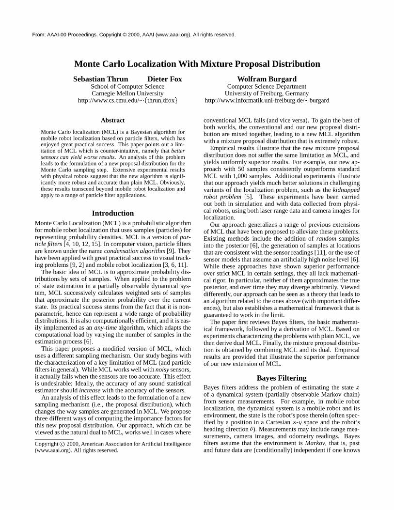
Figure 1: Global localization of a mobile robot using MCL (10,000 samples).

the current state.The key idea of Bayes filtering is to estimate a probability

density over the state space conditioned on the data. Thisposterior is typically called thebeliefand is denoted

Bel(x(t)) = p(x(t)jd(0:::t))

Herex denotes the state,x(t) is the state at timet, andd(0:::t)

denotes the data starting at time0 up to time t. For mo-bile robots, we distinguish two types of data:perceptual datasuch as laser range measurements, andodometry dataor con-trols, which carries information about robot motion. Denot-ing the former byo (for observation) and the latter bya (foraction), we have

Bel(x(t)) = p(x(t)jo(t); a(t�1); o(t�1); a(t�2) : : : ; o(0)) (1)

Without loss of generality, we assume that observations andactions arrive in an alternating sequence.

Bayes filters estimate the beliefrecursively. Theinitial be-lief characterizes the initial knowledge about the system state.In the absence of such, it is typically initialized by auni-form distributionover the state space. In mobile robotics, thestate estimation without initial knowledge is called thegloballocalization problem—which will be the focus throughoutmuch of this paper.

To derive a recursive update equation, we observe that Ex-pression (1) can be transformed by Bayes rule to

p(o(t)jx(t); a(t�1); : : : ; o(0)) p(x(t)ja(t�1); : : : ; o(0))

p(o(t)ja(t�1); : : : ; o(0))

Under our Markov assumption,p(o(t)jx(t); a(t�1); : : : ; o(0))can be simplified top(o(t)jx(t)), hence we have

p(o(t)jx(t)) p(x(t)ja(t�1); : : : ; o(0))

p(o(t)ja(t�1); : : : ; o(0))

We will now expand the rightmost term in the denominatorby integrating over the state at timet� 1

p(o(t)jx(t))

p(o(t)ja(t�1); : : : ; o(0))

Zp(x(t)jx(t�1); a(t�1); : : : ; o(0))

p(x(t�1)ja(t�1); : : : ; o(0)) dx(t�1)

Again, we can exploit the Markov assumption to simplifyp(x(t)jx(t�1); a(t�1); : : : ; o(0)) to p(x(t)jx(t�1); a(t�1)). Us-ing the definition of the beliefBel, we obtain the important

recursive equation

Bel(x(t)) =p(o(t)jx(t))

p(o(t)ja(t�1); : : : ; o(0))(2)Z

p(x(t)jx(t�1); a(t�1)) Bel(x(t�1)) dx(t�1)

= �p(o(t)jx(t))

Zp(x(t)jx(t�1); a(t�1))Bel(x(t�1))dx(t�1)

where� is a normalization constant. This equation is of cen-tral importance, as it is the basis for various MCL algorithmsstudied here.

We notice that to implement (2), one needs to know threedistributions: the initial beliefBel(x(0)) (e.g., uniform), thenext state probabilitiesp(x(t)jx(t�1); a(t�1)), and the percep-tual likelihoodp(o(t)jx(t)). MCL employs specific next stateprobabilitiesp(x(t)jx(t�1); a(t�1)) and perceptual likelihoodmodelsp(o(t)jx(t)) that describe robot motion and percep-tion probabilistically. Such models are described in detailelsewhere [7].

Monte Carlo LocalizationThe idea of MCL (and other particle filter algorithms) is torepresent the beliefBel(x) by a set ofm weighted samplesdistributed according toBel(x):

Bel(x) = fxi; wigi=1;:::;m

Here eachxi is a sample (a state), andwi is a non-negativenumerical factor (weight) calledimportance factors, whichsums up to one over alli.

In global mobile robot localization, theinitial belief is a setof poses drawn according to a uniform distribution over therobot’s universe, and annotated by the uniform importancefactor 1

m. The recursive update is realized in three steps.

1. Samplex(t�1)i �Bel(x(t�1)) using importance samplingfrom the (weighted) sample set representingBel(x(t�1)).

2. Samplex(t)i �p(x(t)jx(t�1)i ; a(t�1)). Obviously, the pair

hx(t)i ; x

(t�1)i i is distributed according to the product dis-

tribution

q(t) := p(x(t)jx(t�1); a(t�1))�Bel(x(t�1)) (3)

which is commonly calledproposal distribution.

0 20 40 60 80 100step

100

200

300

400

500

600

erro

r (i

n c

enti

met

er)

100 samples

1,000 samples

10,000 samples

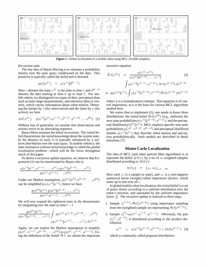
Figure 2: Average error of MCL as a function of the number ofrobot steps/measurements.

3. To offset the difference between the proposal distributionand the desired distribution (c.f., Equation (2))

� p(o(t)jx(t))p(x(t)jx(t�1); a(t�1))Bel(x(t�1)) (4)

the sample is weighted by the quotient

� p(o(t)jx(t)i )p(x

(t)i jx

(t�1)i ; a(t�1))Bel(x

(t�1)i )

Bel(x(t�1)i ) p(x

(t)i jx

(t�1)i ; a(t�1))

/ p(o(t)jx(t)i ) = wi (5)

This is exactly the new (non-normalized) importance factorwi.

After the generation ofm samples, the new importance fac-tors are normalized so that they sum up to 1 (hence definea probability distribution). It is known [17] that under mildassumptions (which hold in our work), the sample set con-verges to the true posteriorBel(x(t)) asm goes to infinity,with a convergence speed inO( 1p

m). The speed may vary by

a constant factor, which depends on the proposal distributionand can be significant.

ExamplesFigure 1 shows an example of MCL in the context of local-izing a mobile robot globally in an office environment. Thisrobot is equipped with sonar range finders, and it is also givena map of the environment. In Figure 1a, the robot is globallyuncertain; hence the samples are spread uniformly trough thefree-space (projected into 2D). Figure 1b shows the sampleset after approximately 1 meter of robot motion, at whichpoint MCL has disambiguated the robot’s position up to asingle symmetry. Finally, after another 2 meters of robot mo-tion the ambiguity is resolved, and the robot knows where itis. The majority of samples is now centered tightly aroundthe correct position, as shown in Figure 1c.

Unfortunately, data collected from a physical robot makesit impossible to freely vary the level of noise in sensing. Fig-ure 2 shows results obtained from a robot simulation, model-ing a B21 robot localizing an object in 3D with a mono cam-era while moving around. The noise simulation includes asimulation of measurement noise, false positives (phantoms)and false negatives (failures to detect the target object). MCLis directly applicable; with the added advantage that we canvary the level of noise arbitrarily. Figure 2 shows system-atic error curves for MCL in global localization for different

50.40.30.20.10.7.5.4.3.2.1.sensor noise level (in %)

100

200

300

400

500

erro

r (i

n c

enti

met

er)

50.40.30.20.10.7.5.4.3.2.1.

MCL

(dashed: high error model)

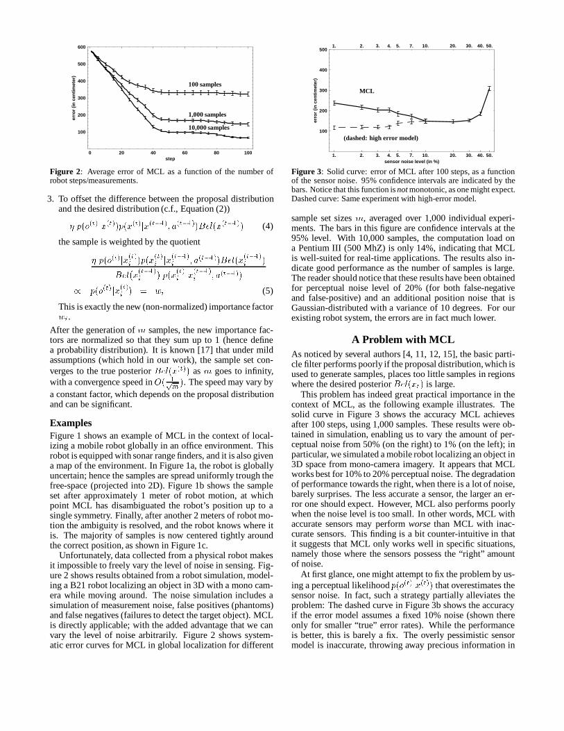
Figure 3: Solid curve: error of MCL after 100 steps, as a functionof the sensor noise. 95% confidence intervals are indicated by thebars. Notice that this function isnotmonotonic, as one might expect.Dashed curve: Same experiment with high-error model.

sample set sizesm, averaged over 1,000 individual experi-ments. The bars in this figure are confidence intervals at the95% level. With 10,000 samples, the computation load ona Pentium III (500 MhZ) is only 14%, indicating that MCLis well-suited for real-time applications. The results also in-dicate good performance as the number of samples is large.The reader should notice that these results have been obtainedfor perceptual noise level of 20% (for both false-negativeand false-positive) and an additional position noise that isGaussian-distributed with a variance of 10 degrees. For ourexisting robot system, the errors are in fact much lower.

A Problem with MCLAs noticed by several authors [4, 11, 12, 15], the basic parti-cle filter performs poorly if the proposal distribution,which isused to generate samples, places toolittle samples in regionswhere the desired posteriorBel(xt) is large.

This problem has indeed great practical importance in thecontext of MCL, as the following example illustrates. Thesolid curve in Figure 3 shows the accuracy MCL achievesafter 100 steps, using 1,000 samples. These results were ob-tained in simulation, enabling us to vary the amount of per-ceptual noise from 50% (on the right) to 1% (on the left); inparticular, we simulated a mobile robot localizing an object in3D space from mono-camera imagery. It appears that MCLworks best for 10% to 20% perceptual noise. The degradationof performance towards the right, when there is a lot of noise,barely surprises. The less accurate a sensor, the larger an er-ror one should expect. However, MCL also performs poorlywhen the noise level is too small. In other words, MCL withaccurate sensors may performworsethan MCL with inac-curate sensors. This finding is a bit counter-intuitive in thatit suggests that MCL only works well in specific situations,namely those where the sensors possess the “right” amountof noise.

At first glance, one might attempt to fix the problem by us-ing a perceptual likelihoodp(o(t)jx(t)) that overestimates thesensor noise. In fact, such a strategy partially alleviates theproblem: The dashed curve in Figure 3b shows the accuracyif the error model assumes a fixed 10% noise (shown thereonly for smaller “true” error rates). While the performanceis better, this is barely a fix. The overly pessimistic sensormodel is inaccurate, throwing away precious information in

50.40.30.20.10.7.5.4.3.2.1.sensor noise level (in %)

100

200

300

400

500

erro

r (i

n c

enti

met

er)

50.40.30.20.10.7.5.4.3.2.1.

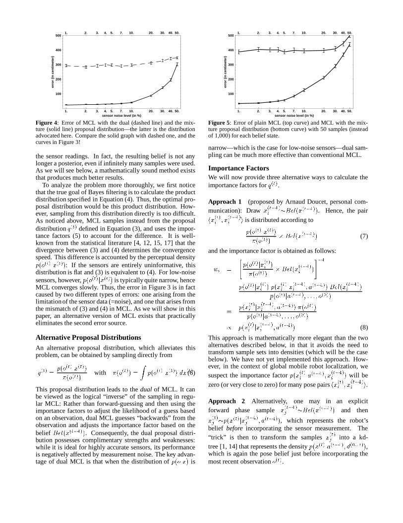
Figure 4: Error of MCL with the dual (dashed line) and the mix-ture (solid line) proposal distribution—the latter is the distributionadvocated here. Compare the solid graph with dashed one, and thecurves in Figure 3!

the sensor readings. In fact, the resulting belief is not anylonger a posterior, even if infinitely many samples were used.As we will see below, a mathematically sound method existsthat produces much better results.

To analyze the problem more thoroughly, we first noticethat the true goal of Bayes filtering is to calculate the productdistribution specified in Equation (4). Thus, the optimal pro-posal distribution would be this product distribution. How-ever, sampling from this distribution directly is too difficult.As noticed above, MCL samples instead from the proposaldistributionq(t) defined in Equation (3), and uses the impor-tance factors (5) to account for the difference. It is well-known from the statistical literature [4, 12, 15, 17] that thedivergence between (3) and (4) determines the convergencespeed. This difference is accounted by the perceptual densityp(o(t)jx(t)): If the sensors are entirely uninformative, thisdistribution is flat and (3) is equivalent to (4). For low-noisesensors, however,p(o(t)jx(t)) is typically quite narrow, henceMCL converges slowly. Thus, the error in Figure 3 is in factcaused by two different types of errors: one arising from thelimitationof the sensor data (=noise), and one that arises fromthe mismatch of (3) and (4) in MCL. As we will show in thispaper, an alternative version of MCL exists that practicallyeliminates the second error source.

Alternative Proposal DistributionsAn alternative proposal distribution, which alleviates thisproblem, can be obtained by sampling directly from

�q(t) =p(o(t)jx(t))

�(o(t))with �(o(t)) =

Zp(o(t)jx(t)) dx(t)(6)

This proposal distribution leads to thedual of MCL. It canbe viewed as the logical “inverse” of the sampling in regu-lar MCL: Rather than forward-guessing and then using theimportance factors to adjust the likelihood of a guess basedon an observation, dual MCL guesses “backwards” from theobservation and adjusts the importance factor based on thebelief Bel(x(t�1)). Consequently, the dual proposal distri-bution possesses complimentary strengths and weaknesses:while it is ideal for highly accurate sensors, its performanceis negatively affected by measurement noise. The key advan-tage of dual MCL is that when the distribution ofp(ojx) is

50.40.30.20.10.7.5.4.3.2.1.sensor noise level (in %)

100

200

300

400

500

erro

r (i

n c

enti

met

er)

50.40.30.20.10.7.5.4.3.2.1.

Figure 5: Error of plain MCL (top curve) and MCL with the mix-ture proposal distribution (bottom curve) with 50 samples (insteadof 1,000) for each belief state.

narrow—which is the case for low-noise sensors—dual sam-pling can be much more effective than conventional MCL.

Importance FactorsWe will now provide three alternative ways to calculate theimportance factors for�q(t).

Approach 1 (proposed by Arnaud Doucet, personal com-munication): Drawx

(t�1)i �Bel(x(t�1)). Hence, the pair

hx(t)i ; x(t�1)i i is distributed according to

p(o(t)jx(t))

�(o(t))� Bel(x(t�1)) (7)

and the importance factor is obtained as follows:

wi =

"p(o(t)jx(t)i )

�(o(t))�Bel(x(t�1)i )

#�1

p(o(t)jx(t)i ) p(x(t)i jx(t�1)i ; a(t�1)) Bel(x(t�1)i )

p(o(t)ja(t�1); : : : ; o(0))

=p(x

(t)i jx

(t�1)i ; a(t�1)) �(o(t))

p(o(t)ja(t�1); : : : ; o(0))

/ p(x(t)i jx

(t�1)i ; a(t�1)) (8)

This approach is mathematically more elegant than the twoalternatives described below, in that it avoids the need totransform sample sets into densities (which will be the casebelow). We have not yet implemented this approach. How-ever, in the context of global mobile robot localization, wesuspect the importance factorp(x(t)i ja(t�1); x

(t�1)i ) will be

zero (or very close to zero) for many pose pairshx(t)i ; x

(t�1)i i.

Approach 2 Alternatively, one may in an explicitforward phase samplex(t�1)j �Bel(x(t�1)) and then

x(t)j �p(x(t)jx

(t�1)j ; a(t�1)), which represents the robot’s

belief before incorporating the sensor measurement. The“trick” is then to transform the samplesx(t)j into a kd-tree [1, 14] that represents the densityp(x(t)ja(t�1); d(0:::t)),which is again the pose belief just before incorporating themost recent observationo(t).

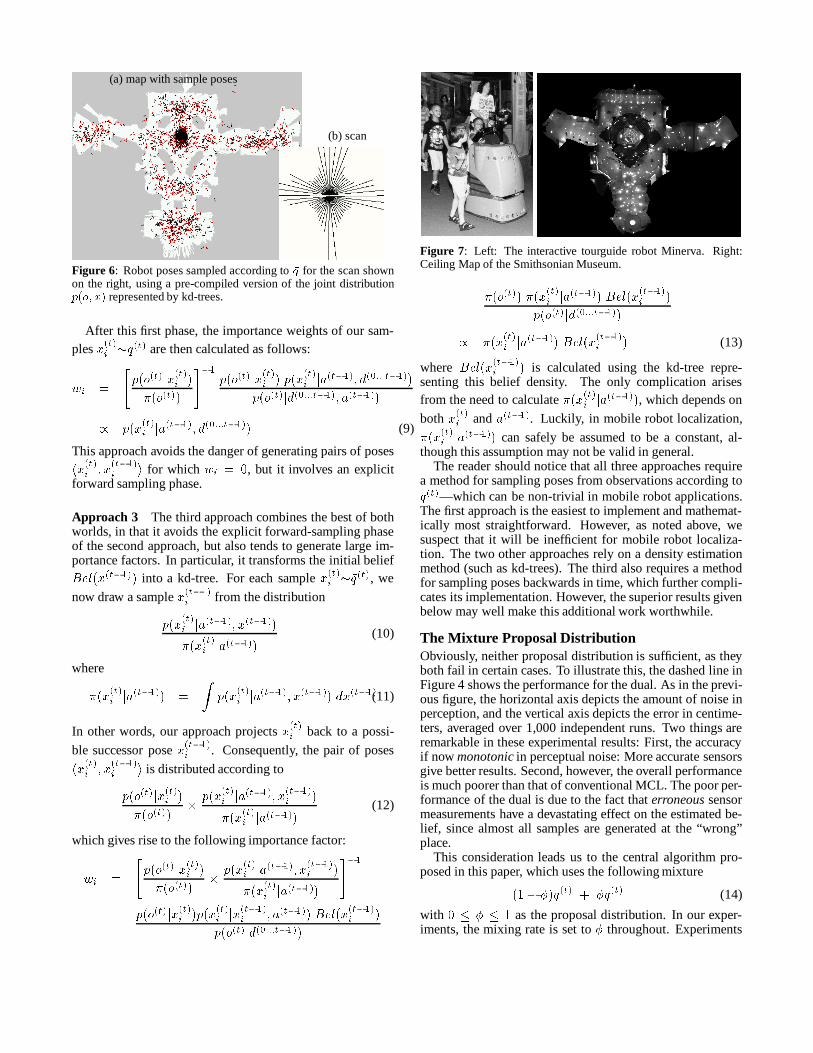
(a) map with sample poses

(b) scan

Figure 6: Robot poses sampled according to�q for the scan shownon the right, using a pre-compiled version of the joint distributionp(o; x) represented by kd-trees.

After this first phase, the importance weights of our sam-plesx(t)i ��q(t) are then calculated as follows:

wi =

"p(o(t)jx

(t)i )

�(o(t))

#�1p(o(t)jx

(t)i ) p(x

(t)i ja(t�1); d(0:::t�1))

p(o(t)jd(0:::t�1); a(t�1))

/ p(x(t)i ja(t�1); d(0:::t�1)) (9)

This approach avoids the danger of generating pairs of poseshx

(t)i ; x

(t�1)i i for which wi = 0, but it involves an explicit

forward sampling phase.

Approach 3 The third approach combines the best of bothworlds, in that it avoids the explicit forward-sampling phaseof the second approach, but also tends to generate large im-portance factors. In particular, it transforms the initial beliefBel(x(t�1)) into a kd-tree. For each samplex(t)i ��q(t), we

now draw a samplex(t�1)i from the distribution

p(x(t)i ja(t�1); x(t�1))

�(x(t)i ja(t�1))

(10)

where

�(x(t)i ja(t�1)) =

Zp(x

(t)i ja(t�1); x(t�1)) dx(t�1)(11)

In other words, our approach projectsx(t)i back to a possi-

ble successor posex(t�1)i . Consequently, the pair of poses

hx(t)i ; x

(t�1)i i is distributed according to

p(o(t)jx(t)i )

�(o(t))�

p(x(t)i ja(t�1); x(t�1)i )

�(x(t)i ja(t�1))(12)

which gives rise to the following importance factor:

wi =

"p(o(t)jx

(t)i )

�(o(t))�

p(x(t)i ja(t�1); x

(t�1)i )

�(x(t)i ja(t�1))

#�1

p(o(t)jx(t)i )p(x(t)i jx(t�1)i ; a(t�1)) Bel(x(t�1)i )

p(o(t)jd(0:::t�1))

Figure 7: Left: The interactive tourguide robot Minerva. Right:Ceiling Map of the Smithsonian Museum.

=�(o(t)) �(x

(t)i ja(t�1)) Bel(x

(t�1)i )

p(o(t)jd(0:::t�1))

/ �(x(t)i ja(t�1)) Bel(x

(t�1)i ) (13)

where Bel(x(t�1)i ) is calculated using the kd-tree repre-

senting this belief density. The only complication arisesfrom the need to calculate�(x(t)i ja(t�1)), which depends on

bothx(t)i anda(t�1). Luckily, in mobile robot localization,

�(x(t)i ja(t�1)) can safely be assumed to be a constant, al-though this assumption may not be valid in general.

The reader should notice that all three approaches requirea method for sampling poses from observations according to�q(t)—which can be non-trivial in mobile robot applications.The first approach is the easiest to implement and mathemat-ically most straightforward. However, as noted above, wesuspect that it will be inefficient for mobile robot localiza-tion. The two other approaches rely on a density estimationmethod (such as kd-trees). The third also requires a methodfor sampling poses backwards in time, which further compli-cates its implementation. However, the superior results givenbelow may well make this additional work worthwhile.

The Mixture Proposal DistributionObviously, neither proposal distribution is sufficient, as theyboth fail in certain cases. To illustrate this, the dashed line inFigure 4 shows the performance for the dual. As in the previ-ous figure, the horizontal axis depicts the amount of noise inperception, and the vertical axis depicts the error in centime-ters, averaged over 1,000 independent runs. Two things areremarkable in these experimental results: First, the accuracyif now monotonicin perceptual noise: More accurate sensorsgive better results. Second, however, the overall performanceis much poorer than that of conventional MCL. The poor per-formance of the dual is due to the fact thaterroneoussensormeasurements have a devastating effect on the estimated be-lief, since almost all samples are generated at the “wrong”place.

This consideration leads us to the central algorithm pro-posed in this paper, which uses the following mixture

(1� �)q(t) + ��q(t) (14)

with 0 � � � 1 as the proposal distribution. In our exper-iments, the mixing rate is set to� throughout. Experiments

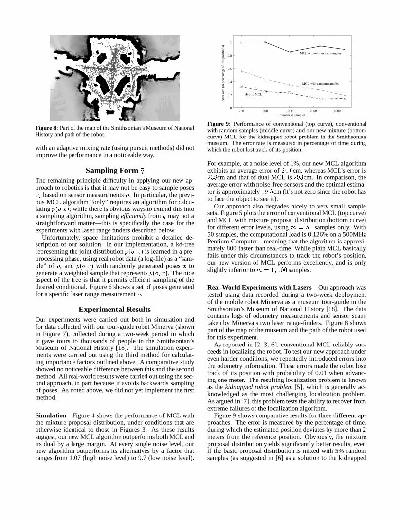
Figure 8: Part of the map of the Smithsonian’s Museum of NationalHistory and path of the robot.

with an adaptive mixing rate (using pursuit methods) did notimprove the performance in a noticeable way.

Sampling Form �q

The remaining principle difficulty in applying our new ap-proach to robotics is that it may not be easy to sample posesxi based on sensor measurementso. In particular, the previ-ous MCL algorithm “only” requires an algorithm for calcu-latingp(ojx); while there is obvious ways to extend this intoa sampling algorithm, samplingefficientlyfrom �q may not astraightforward matter—this is specifically the case for theexperiments with laser range finders described below.

Unfortunately, space limitations prohibit a detailed de-scription of our solution. In our implementation, a kd-treerepresenting the joint distributionp(o; x) is learned in a pre-processing phase, using real robot data (a log-file) as a “sam-ple” of o, andp(ojx) with randomly generated posesx togenerate a weighted sample that representsp(o; x). The niceaspect of the tree is that it permits efficient sampling of thedesired conditional. Figure 6 shows a set of poses generatedfor a specific laser range measuremento.

Experimental ResultsOur experiments were carried out both in simulation andfor data collected with our tour-guide robot Minerva (shownin Figure 7), collected during a two-week period in whichit gave tours to thousands of people in the Smithsonian’sMuseum of National History [18]. The simulation experi-ments were carried out using the third method for calculat-ing importance factors outlined above. A comparative studyshowed no noticeable difference between this and the secondmethod. All real-world results were carried out using the sec-ond approach, in part because it avoids backwards samplingof poses. As noted above, we did not yet implement the firstmethod.

Simulation Figure 4 shows the performance of MCL withthe mixture proposal distribution, under conditions that areotherwise identical to those in Figures 3. As these resultssuggest, our new MCL algorithm outperforms both MCL andits dual by a large margin. At every single noise level, ournew algorithm outperforms its alternatives by a factor thatranges from 1.07 (high noise level) to 9.7 (low noise level).

0

0.2

0.4

0.6

0.8

1

250 500 1000 2000 4000number of samples

Hybrid MCL

MCL without random samples

MCL with random samples

erro

r ra

te (

in p

erce

ntag

e of

lost

pos

ition

s)

Figure 9: Performance of conventional (top curve), conventionalwith random samples (middle curve) and our new mixture (bottomcurve) MCL for the kidnapped robot problem in the Smithsonianmuseum. The error rate is measured in percentage of time duringwhich the robot lost track of its position.

For example, at a noise level of 1%, our new MCL algorithmexhibits an average error of24:6cm, whereas MCL’s error is238cm and that of dual MCL is293cm. In comparison, theaverage error with noise-free sensors and the optimal estima-tor is approximately19:5cm (it’s not zero since the robot hasto face the object to see it).

Our approach also degrades nicely to very small samplesets. Figure 5 plots the error of conventional MCL (top curve)and MCL with mixture proposal distribution (bottom curve)for different error levels, usingm = 50 samples only. With50 samples, the computational load is 0.126% on a 500MHzPentium Computer—meaning that the algorithm is approxi-mately 800 faster than real-time. While plain MCL basicallyfails under this circumstances to track the robot’s position,our new version of MCL performs excellently, and is onlyslightly inferior tom = 1; 000 samples.

Real-World Experiments with Lasers Our approach wastested using data recorded during a two-week deploymentof the mobile robot Minerva as a museum tour-guide in theSmithsonian’s Museum of National History [18]. The datacontains logs of odometry measurements and sensor scanstaken by Minerva’s two laser range-finders. Figure 8 showspart of the map of the museum and the path of the robot usedfor this experiment.

As reported in [2, 3, 6], conventional MCL reliably suc-ceeds in localizing the robot. To test our new approach undereven harder conditions, we repeatedly introduced errors intothe odometry information. These errors made the robot losetrack of its position with probability of 0.01 when advanc-ing one meter. The resulting localization problem is knownas thekidnapped robot problem[5], which is generally ac-knowledged as the most challenging localization problem.As argued in [7], this problem tests the ability to recover fromextreme failures of the localization algorithm.

Figure 9 shows comparative results for three different ap-proaches. The error is measured by the percentage of time,during which the estimated position deviates by more than 2meters from the reference position. Obviously, the mixtureproposal distribution yields significantly better results, evenif the basic proposal distribution is mixed with 5% randomsamples (as suggested in [6] as a solution to the kidnapped

0

500

1000

1500

2000

2500

3000

3500

4000

4500

0 500 1000 1500 2000 2500 3000 3500 4000

Dis

tanc

e [c

m]

Time [sec]

Standard MCLMixture MCL

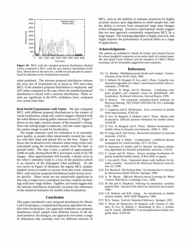
Figure 10: MCL with the standard proposal distribution (dashedcurve) compared to MCL with the new mixture distribution (solidline). Shown here is the error for a 4,000-second episode of camera-based localization in the Smithsonian museum.

robot problem). The mixture proposal distribution reducesthe error rate of localization by as much as 70% more thanMCL if the standard proposal distribution is employed; and32% when compared to the case where the standard proposaldistribution is mixed with a uniform distribution. These re-sults are significant at the 95% confidence level, evaluatedover actual robot data.

Real-World Experiments with Vision We also comparedMCL with different proposal distributions in the context ofvisual localization, using only camera imagery obtained withthe robot Minerva during public museum hours [2]. Figure 7shows on the right a texture mosaic of the museum’s ceiling.Since the ceiling height is unknown, only the center region inthe camera image is used for localization.

The image sequence used for evaluation is of extremelypoor quality, as people often intentionally covered the cam-era with their hand and placed dirt on the lens. Figure 10shows the localization error obtained when using vision only(calculated using the localization results from the laser asground truth). The data covers a period of approximately4,000 seconds, during which MCL processes a total of 20,740images. After approximately 630 seconds, a drastic error inthe robot’s odometry leads to a loss of the position (whichis an instance of the kidnapped robot problem). As thetwo curves in Figure 10 illustrate, the regular MCL sampler(dashed curve) is unable to recover from this event, whereasMCL with mixture proposal distribution (solid curve) recov-ers quickly. These result are not statistically significant inthat only a single run is considered, but they confirm our find-ings with laser range finders. Together, our result suggest thatthe mixture distribution drastically increases the robustnessof the statistical estimator for mobile robot localization.

ConclusionThis paper introduced a new proposal distribution for MonteCarlo localization, a randomized Bayesian algorithm for mo-bile robot localization. Our approach combines two proposaldistribution which sample from different factors of the de-sired posterior. By doing so, our approach overcomes a rangeof limitations that currently exist for different versions of

MCL, such as the inability to estimate posteriors for highlyaccurate sensors,poor degradation to small sample sets, andthe ability to recover from unexpected large state changes(robot kidnapping). Extensive experimental results suggestthat our new approach consistently outperforms MCL by alarge margin. The resulting algorithm is highly practical, andmight improve the performance of particle filters in a rangeof applications.

AcknowledgmentsThe authors are indebted to Nando de Freitas and Arnaud Doucetfor whose insightful comments on an earlier draft of a related paper.We also thank Frank Dellaert and the members of CMU’s RobotLearning Lab for invaluable suggestions and comments.

References[1] J.L. Bentley. Multidimensional divide and conquer.Commu-

nications of the ACM, 23(4), 1980.[2] F. Dellaert, W. Burgard, D. Fox, and S. Thrun. Using the con-

densation algorithm for robust, vision-based mobile robot lo-calization. CVPR-99.

[3] J. Denzler, B. Heigl, and H. Niemann. Combining com-puter graphics and computer vision for probabilistic self-localization. Rochester University, Internal Report, 1999.

[4] A Doucet. On sequential simulation-based methods forBayesian filtering. TR CUED/F-INFENG/TR 310, CambridgeUniv., 1998.

[5] S. Engelson and D. McDermott. Error correction in mobilerobot map learning. ICRA-92.

[6] D. Fox, W. Burgard, F. Dellaert, and S. Thrun. Monte carlolocalization: Efficient position estimation for mobile robots.AAAI-99.

[7] D. Fox, W. Burgard, and S. Thrun. Markov localization formobile robots in dynamic environments.JAIR11, 1999.

[8] R. Fung and B. Del Favero. Backward simulation in bayesiannetworks. UAI-94.

[9] M. Isard and A. Blake. Condensation: conditional densitypropagation for visual tracking.IJCV, In Press.

[10] K. Kanazawa, D. Koller, and S.J. Russell. Stochastic simula-tion algorithms for dynamic probabilistic networks. UAI-95.

[11] S. Lenser and M. Veloso. Sensor resetting localization forpoorly modelled mobile robots. ICRA-2000, to appear.

[12] J. Liu and R. Chen. Sequential monte carlo methods for dy-namic systems.Journal of the American Statistical Associa-tion, 93, 1998.

[13] P.S. Maybeck. The Kalman filter: An introduction to concepts.In Autonomous Robot Vehicles. Springer, 1990.

[14] A. W. Moore. Efficient Memory-based Learning for RobotControl. PhD thesis, Cambridge Univ., 1990.

[15] M. Pitt and N. Shephard. Filtering via simulation: auxiliaryparticle filter.Journal of the American Statistical Association,1999.

[16] L.R. Rabiner and B.H. Juang. An introduction to hiddenmarkov models.IEEE ASSP Magazine, 1986.

[17] M.A. Tanner.Tools for Statistical Inference. Springer, 1993.[18] S. Thrun, M. Bennewitz, W. Burgard, A.B. Cremers, F. Del-

laert, D. Fox, D. Hahnel, C. Rosenberg, N. Roy, J. Schulte,and D. Schulz. MINERVA: A second generation mobile tour-guide robot. ICRA-99.