Embed Size (px)
Citation preview
Monte Carlo Markov Chain Analysis ofCMB + LSS experimental data
within theEffective Field Theory of Inflation
Claudio [email protected]
Dipartimento di Fisica – Universita Milano–Bicocca
C.D., H.J. de Vega, N. Sanchez, astro-ph/0703417
Paris 17/05/2007 – p. 1/21

Outline of the talk
• Monte Carlo Markov Chains and cosmological parameters
• The COSMOMC program
• Current CMB and LSS data and ΛCDM model
• Effective Field Theory of Inflation
• Trinomial new inflation
• Trinomial chaotic inflation
• Summary and conclusions
Paris 17/05/2007 – p. 2/21

Outline of the talk
• Monte Carlo Markov Chains and cosmological parameters
• The COSMOMC program
• Current CMB and LSS data and ΛCDM model
• Effective Field Theory of Inflation
• Trinomial new inflation
• Trinomial chaotic inflation
• Summary and conclusions
Paris 17/05/2007 – p. 2/21
Outline of the talk
• Monte Carlo Markov Chains and cosmological parameters
• The COSMOMC program
• Current CMB and LSS data and ΛCDM model
• Effective Field Theory of Inflation
• Trinomial new inflation
• Trinomial chaotic inflation
• Summary and conclusions
Paris 17/05/2007 – p. 2/21

Outline of the talk
• Monte Carlo Markov Chains and cosmological parameters
• The COSMOMC program
• Current CMB and LSS data and ΛCDM model
• Effective Field Theory of Inflation
• Trinomial new inflation
• Trinomial chaotic inflation
• Summary and conclusions
Paris 17/05/2007 – p. 2/21

Outline of the talk
• Monte Carlo Markov Chains and cosmological parameters
• The COSMOMC program
• Current CMB and LSS data and ΛCDM model
• Effective Field Theory of Inflation
• Trinomial new inflation
• Trinomial chaotic inflation
• Summary and conclusions
Paris 17/05/2007 – p. 2/21

Outline of the talk
• Monte Carlo Markov Chains and cosmological parameters
• The COSMOMC program
• Current CMB and LSS data and ΛCDM model
• Effective Field Theory of Inflation
• Trinomial new inflation
• Trinomial chaotic inflation
• Summary and conclusions
Paris 17/05/2007 – p. 2/21

Outline of the talk
• Monte Carlo Markov Chains and cosmological parameters
• The COSMOMC program
• Current CMB and LSS data and ΛCDM model
• Effective Field Theory of Inflation
• Trinomial new inflation
• Trinomial chaotic inflation
• Summary and conclusions
Paris 17/05/2007 – p. 2/21
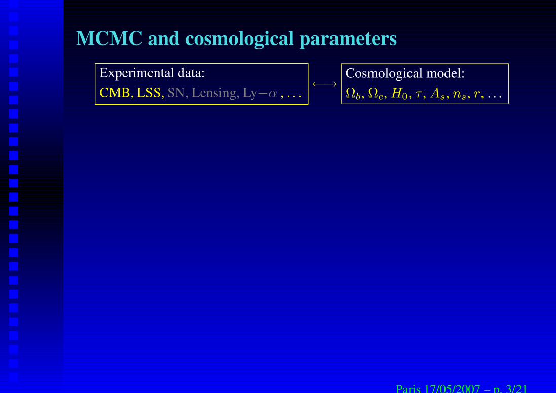
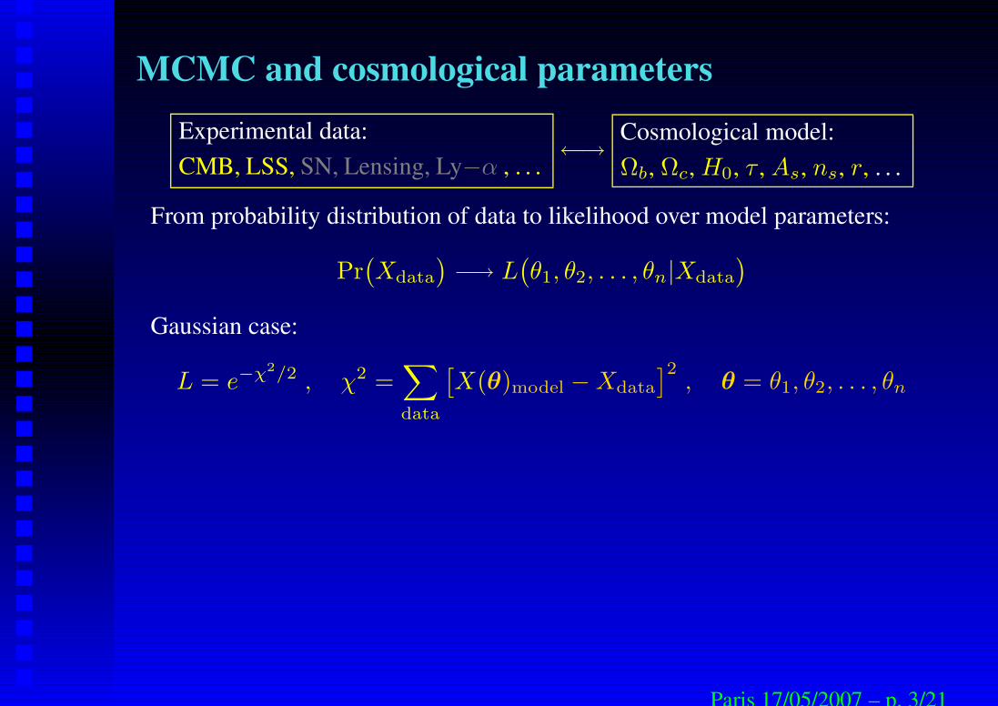
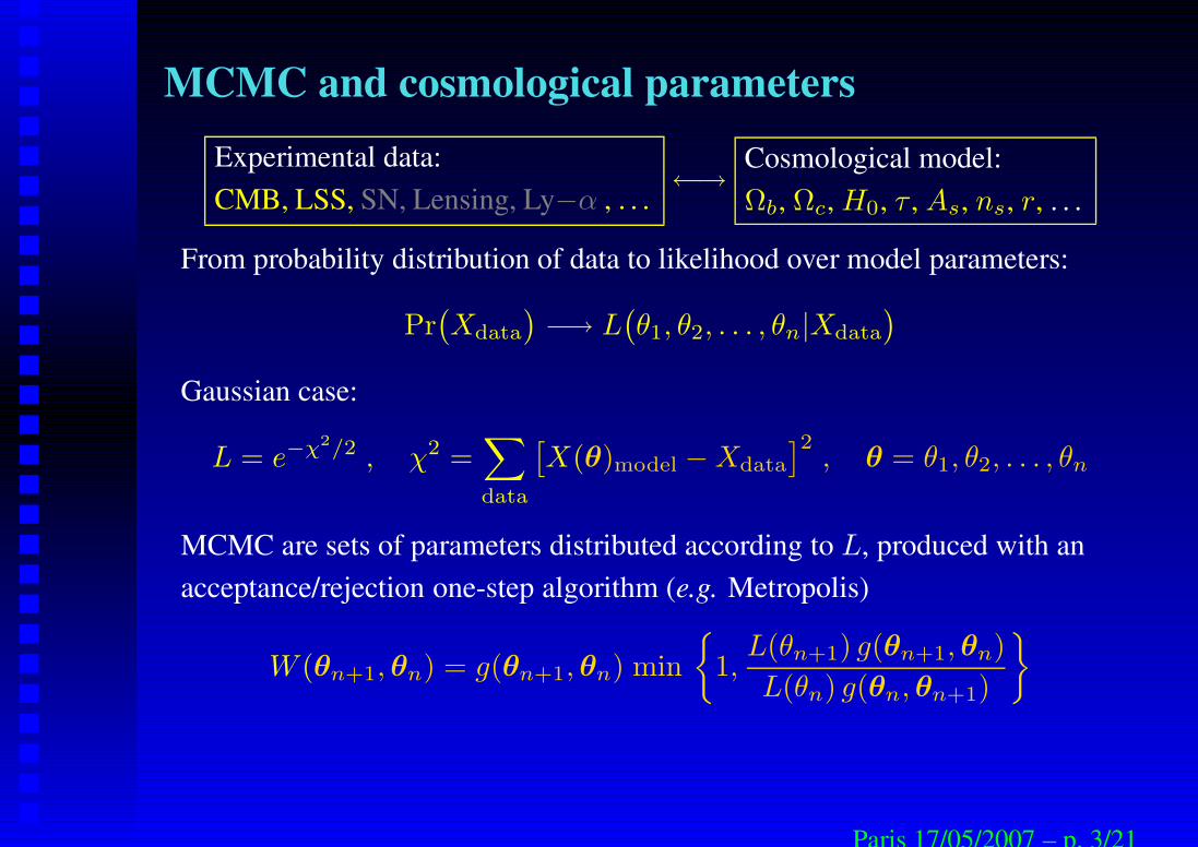
MCMC and cosmological parametersExperimental data:CMB, LSS, SN, Lensing, Ly−α , . . .
←→ Cosmological model:Ωb, Ωc, H0, τ , As, ns, r, . . .
Paris 17/05/2007 – p. 3/21
MCMC and cosmological parametersExperimental data:CMB, LSS, SN, Lensing, Ly−α , . . .
←→ Cosmological model:Ωb, Ωc, H0, τ , As, ns, r, . . .
From probability distribution of data to likelihood over model parameters:
Pr(
Xdata
)
−→ L(
θ1, θ2, . . . , θn|Xdata
)
Gaussian case:
L = e−χ2/2 , χ2 =∑
data
[
X(θ)model −Xdata
]2, θ = θ1, θ2, . . . , θn
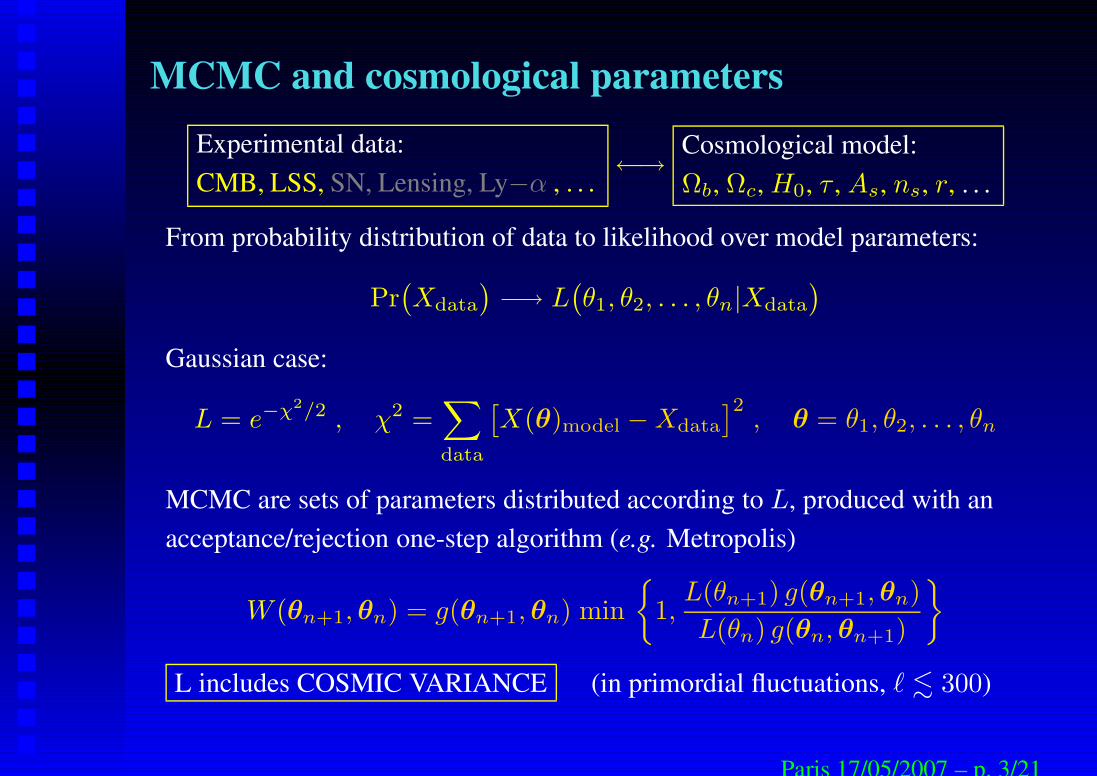
MCMC are sets of parameters distributed according to L, produced with anacceptance/rejection one-step algorithm (e.g. Metropolis)
W (θn+1, θn) = g(θn+1, θn) min
1,L(θn+1) g(θn+1, θn)
L(θn) g(θn, θn+1)
Paris 17/05/2007 – p. 3/21
MCMC and cosmological parametersExperimental data:CMB, LSS, SN, Lensing, Ly−α , . . .
←→ Cosmological model:Ωb, Ωc, H0, τ , As, ns, r, . . .
From probability distribution of data to likelihood over model parameters:
Pr(
Xdata
)
−→ L(
θ1, θ2, . . . , θn|Xdata
)
Gaussian case:
L = e−χ2/2 , χ2 =∑
data
[
X(θ)model −Xdata
]2, θ = θ1, θ2, . . . , θn
MCMC are sets of parameters distributed according to L, produced with anacceptance/rejection one-step algorithm (e.g. Metropolis)
W (θn+1, θn) = g(θn+1, θn) min
1,L(θn+1) g(θn+1, θn)
L(θn) g(θn, θn+1)
L includes COSMIC VARIANCE (in primordial fluctuations, ` . 300)
Paris 17/05/2007 – p. 3/21
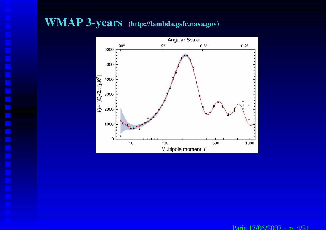
WMAP 3-years (http://lambda.gsfc.nasa.gov)
Paris 17/05/2007 – p. 4/21
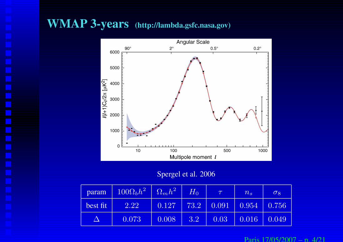
WMAP 3-years (http://lambda.gsfc.nasa.gov)
Spergel et al. 2006
param 100Ωbh2 Ωmh2 H0 τ ns σ8
best fit 2.22 0.127 73.2 0.091 0.954 0.756
∆ 0.073 0.008 3.2 0.03 0.016 0.049
Paris 17/05/2007 – p. 4/21

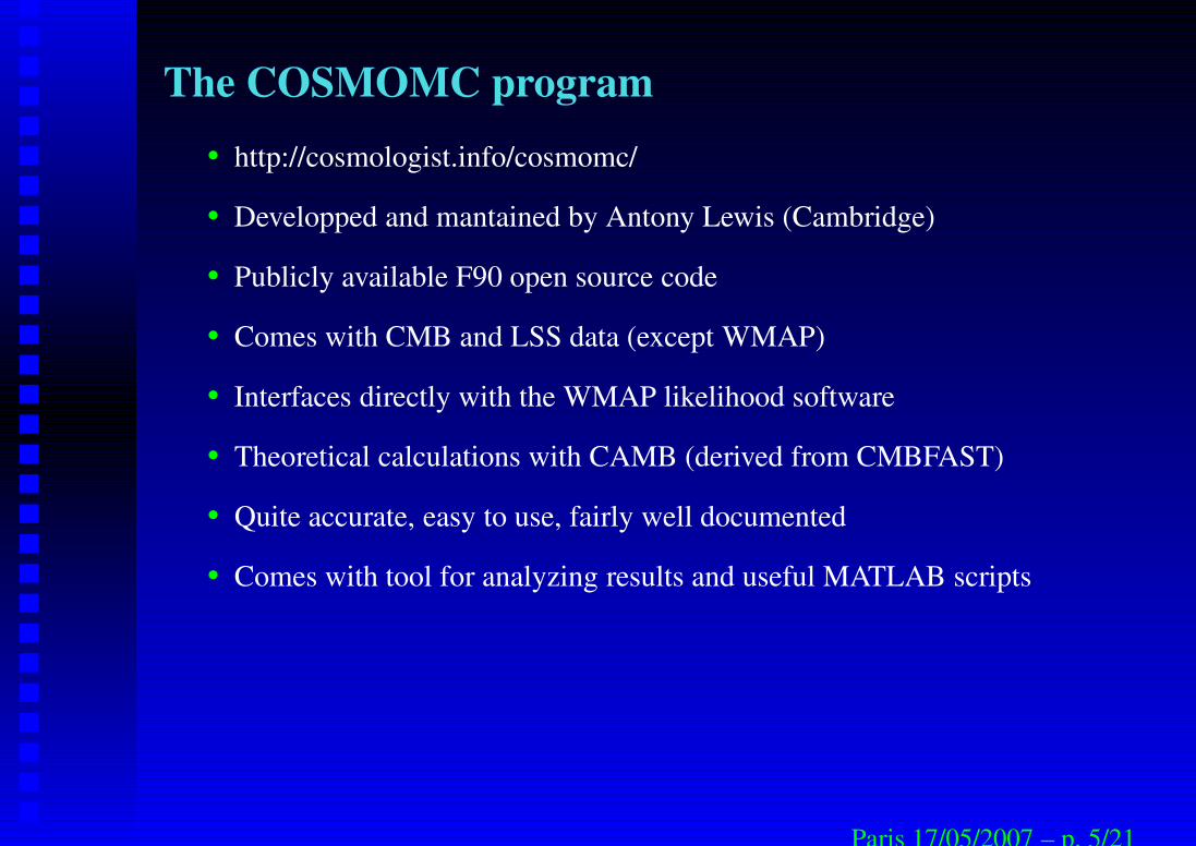
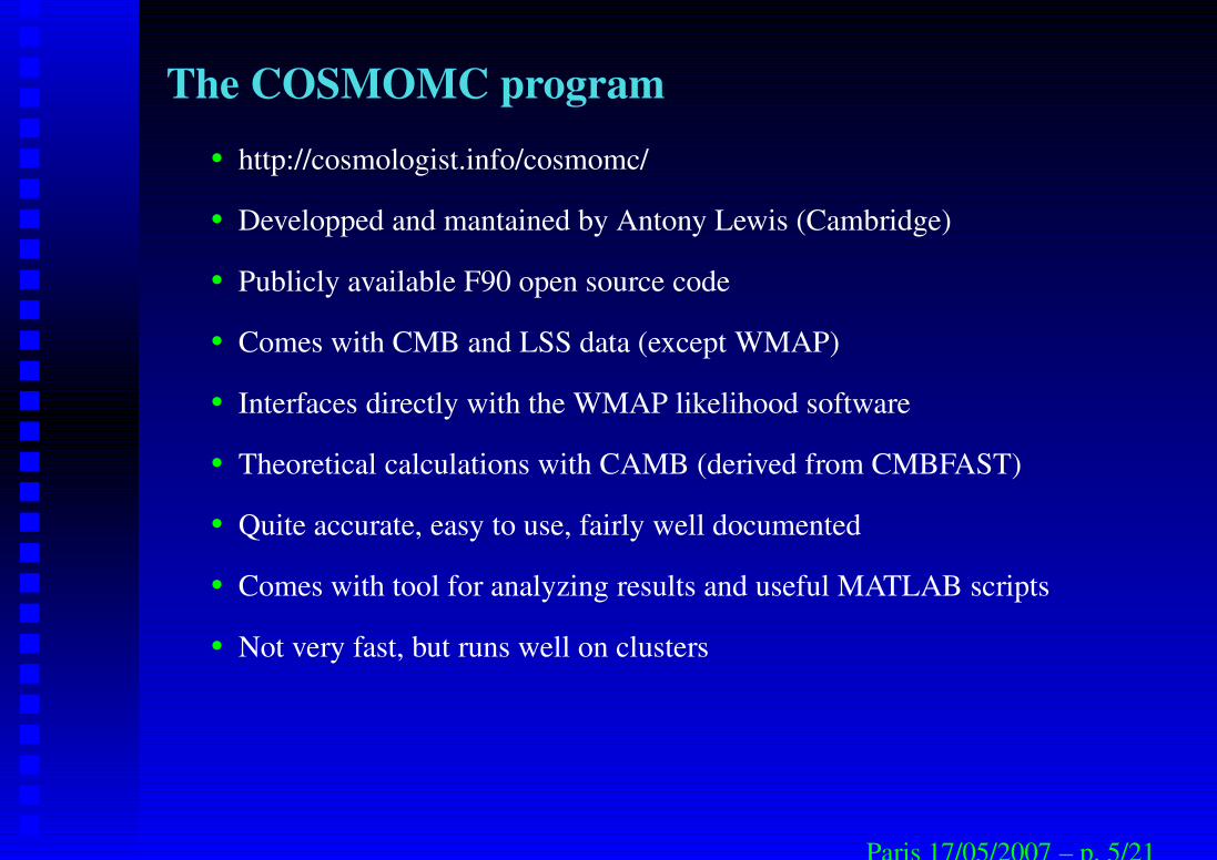
The COSMOMC program• http://cosmologist.info/cosmomc/
• Developped and mantained by Antony Lewis (Cambridge)
• Publicly available F90 open source code
• Comes with CMB and LSS data (except WMAP)
• Interfaces directly with the WMAP likelihood software
• Theoretical calculations with CAMB (derived from CMBFAST)
• Quite accurate, easy to use, fairly well documented
• Comes with tool for analyzing results and useful MATLAB scripts
• Not very fast, but runs well on clusters
Paris 17/05/2007 – p. 5/21
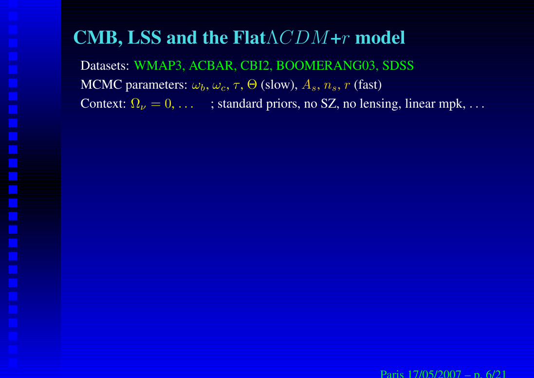
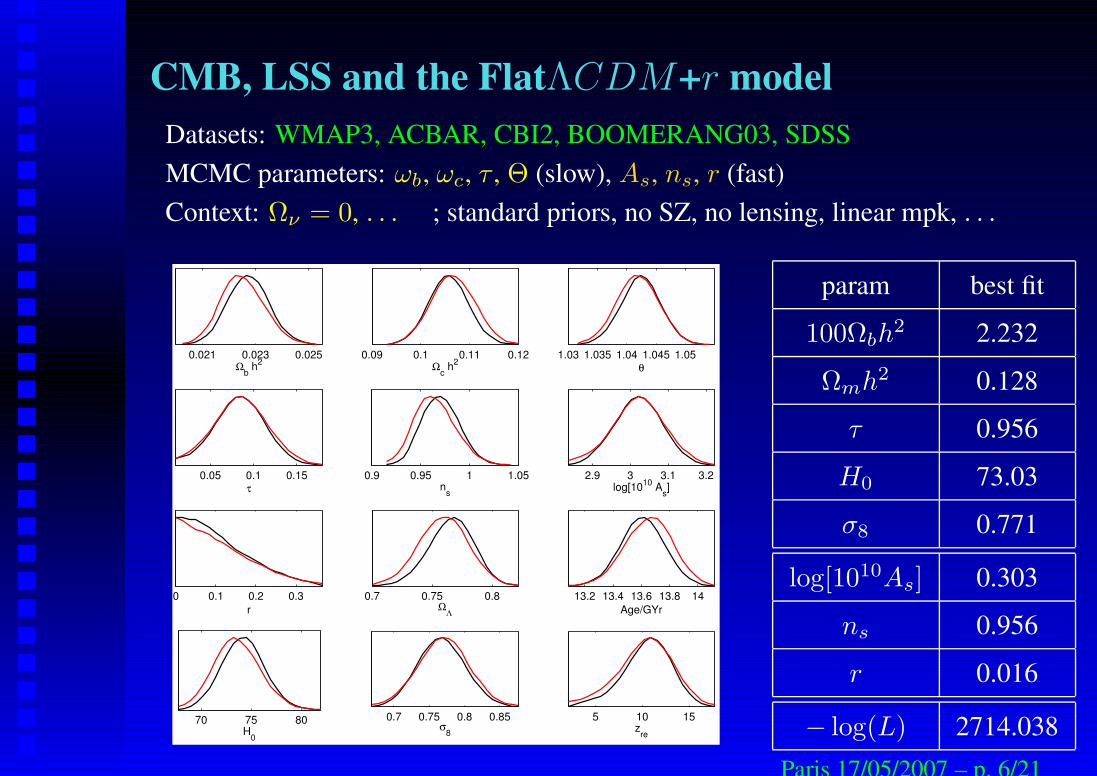
CMB, LSS and the FlatΛCDM+r modelDatasets: WMAP3, ACBAR, CBI2, BOOMERANG03, SDSSMCMC parameters: ωb, ωc, τ , Θ (slow), As, ns, r (fast)Context: Ων = 0, . . . ; standard priors, no SZ, no lensing, linear mpk, . . .
Paris 17/05/2007 – p. 6/21
CMB, LSS and the FlatΛCDM+r modelDatasets: WMAP3, ACBAR, CBI2, BOOMERANG03, SDSSMCMC parameters: ωb, ωc, τ , Θ (slow), As, ns, r (fast)Context: Ων = 0, . . . ; standard priors, no SZ, no lensing, linear mpk, . . .
0.021 0.023 0.025Ωb h2 0.09 0.1 0.11 0.12
Ωc h2 1.03 1.035 1.04 1.045 1.05
θ
0.05 0.1 0.15τ
0.9 0.95 1 1.05ns
2.9 3 3.1 3.2log[1010 As]
0 0.1 0.2 0.3r
0.7 0.75 0.8ΩΛ
13.2 13.4 13.6 13.8 14Age/GYr
0.7 0.75 0.8 0.85σ8
5 10 15zre
70 75 80H0
param best fit
100Ωbh2 2.232
Ωmh2 0.128
τ 0.956
H0 73.03
σ8 0.771
log[1010As] 0.303
ns 0.956
r 0.016
− log(L) 2714.038Paris 17/05/2007 – p. 6/21
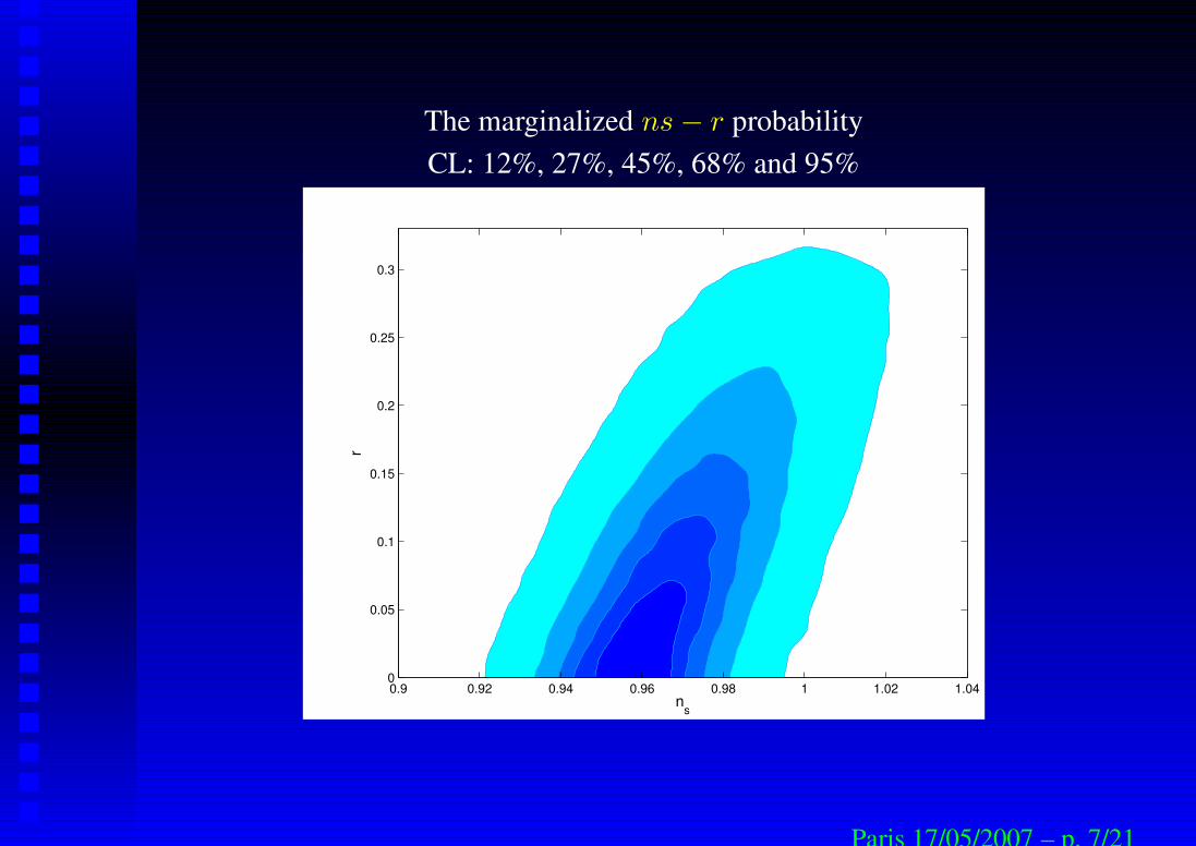
The marginalized ns− r probabilityCL: 12%, 27%, 45%, 68% and 95%
ns
r
0.9 0.92 0.94 0.96 0.98 1 1.02 1.040
0.05
0.1
0.15
0.2
0.25
0.3
Paris 17/05/2007 – p. 7/21
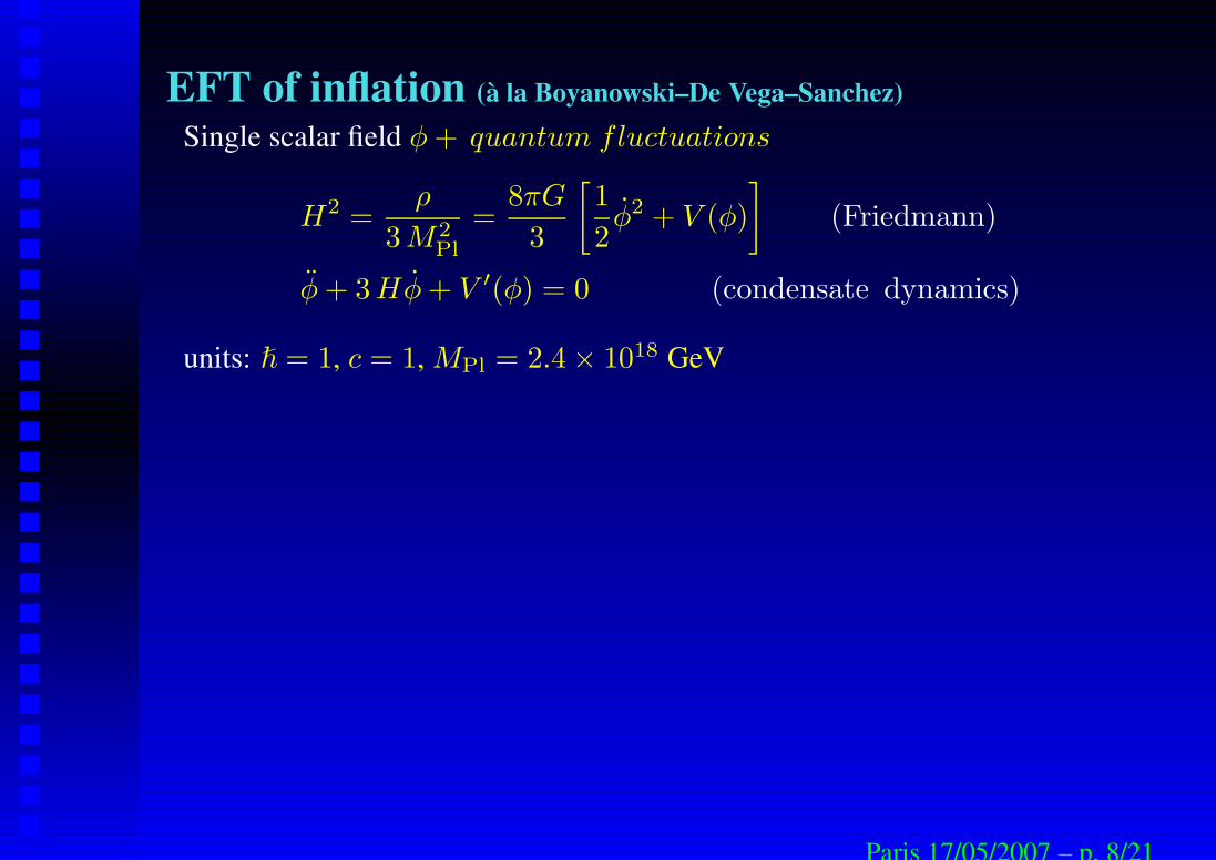
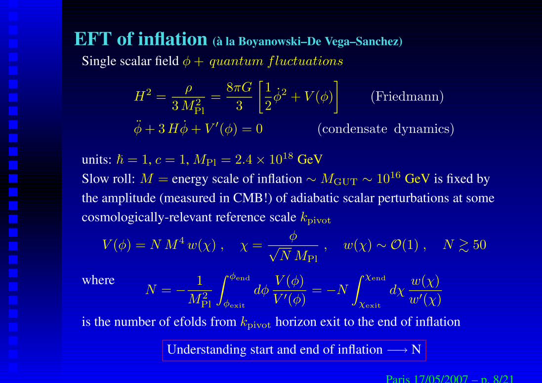
EFT of inflation (à la Boyanowski–De Vega–Sanchez)Single scalar field φ + quantum fluctuations
H2 =ρ
3 M2Pl
=8πG
3
[
1
2φ2 + V (φ)
]
(Friedmann)
φ + 3 Hφ + V ′(φ) = 0 (condensate dynamics)
units: = 1, c = 1, MPl = 2.4× 10¹⁸ GeV
Paris 17/05/2007 – p. 8/21
EFT of inflation (à la Boyanowski–De Vega–Sanchez)Single scalar field φ + quantum fluctuations
H2 =ρ
3 M2Pl
=8πG
3
[
1
2φ2 + V (φ)
]
(Friedmann)
φ + 3 Hφ + V ′(φ) = 0 (condensate dynamics)
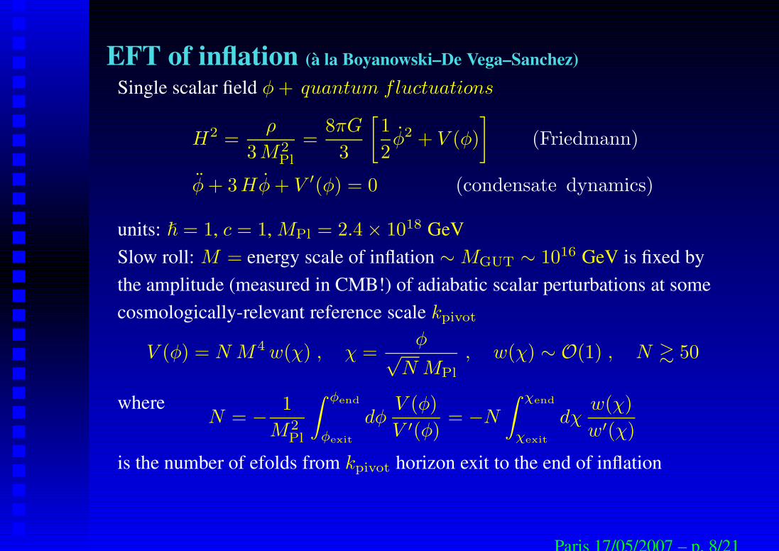
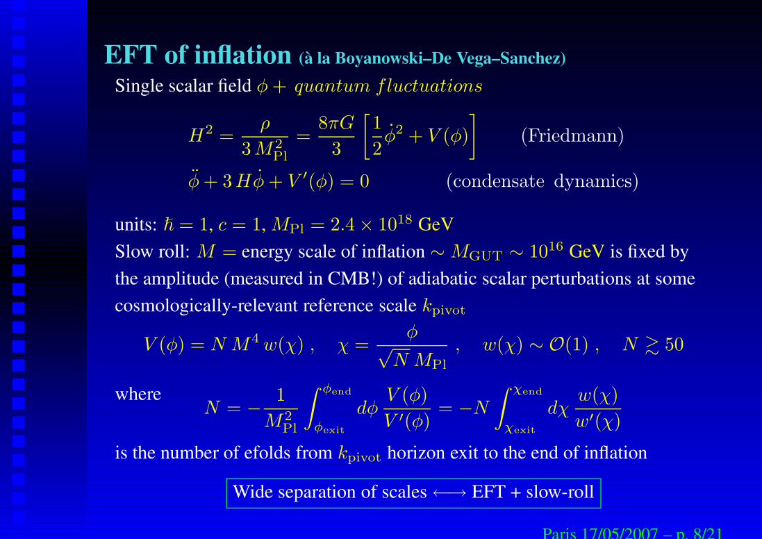
units: = 1, c = 1, MPl = 2.4× 10¹⁸ GeVSlow roll: M = energy scale of inflation ∼MGUT ∼ 1016 GeV is fixed bythe amplitude (measured in CMB!) of adiabatic scalar perturbations at somecosmologically-relevant reference scale kpivot
V (φ) = N M4 w(χ) , χ =φ√
N MPl
, w(χ) ∼ O(1) , N & 50
whereN = − 1
M2Pl
∫ φend
φexit
dφV (φ)
V ′(φ)= −N
∫ χend
χexit
dχw(χ)
w′(χ)
is the number of efolds from kpivot horizon exit to the end of inflation
Paris 17/05/2007 – p. 8/21
EFT of inflation (à la Boyanowski–De Vega–Sanchez)Single scalar field φ + quantum fluctuations
H2 =ρ
3 M2Pl
=8πG
3
[
1
2φ2 + V (φ)
]
(Friedmann)
φ + 3 Hφ + V ′(φ) = 0 (condensate dynamics)
units: = 1, c = 1, MPl = 2.4× 10¹⁸ GeVSlow roll: M = energy scale of inflation ∼MGUT ∼ 1016 GeV is fixed bythe amplitude (measured in CMB!) of adiabatic scalar perturbations at somecosmologically-relevant reference scale kpivot
V (φ) = N M4 w(χ) , χ =φ√
N MPl
, w(χ) ∼ O(1) , N & 50
whereN = − 1
M2Pl
∫ φend
φexit
dφV (φ)
V ′(φ)= −N
∫ χend
χexit
dχw(χ)
w′(χ)
is the number of efolds from kpivot horizon exit to the end of inflation
Wide separation of scales←→ EFT + slow-roll
Paris 17/05/2007 – p. 8/21
EFT of inflation (à la Boyanowski–De Vega–Sanchez)Single scalar field φ + quantum fluctuations
H2 =ρ
3 M2Pl
=8πG
3
[
1
2φ2 + V (φ)
]
(Friedmann)
φ + 3 Hφ + V ′(φ) = 0 (condensate dynamics)
units: = 1, c = 1, MPl = 2.4× 10¹⁸ GeVSlow roll: M = energy scale of inflation ∼MGUT ∼ 1016 GeV is fixed bythe amplitude (measured in CMB!) of adiabatic scalar perturbations at somecosmologically-relevant reference scale kpivot
V (φ) = N M4 w(χ) , χ =φ√
N MPl
, w(χ) ∼ O(1) , N & 50
whereN = − 1
M2Pl
∫ φend
φexit
dφV (φ)
V ′(φ)= −N
∫ χend
χexit
dχw(χ)
w′(χ)
is the number of efolds from kpivot horizon exit to the end of inflation
Understanding start and end of inflation −→ N
Paris 17/05/2007 – p. 8/21
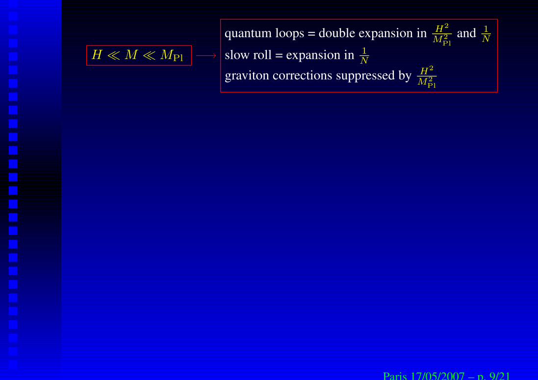
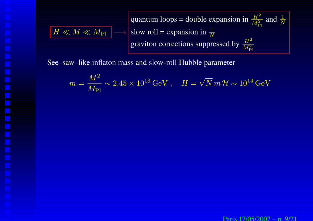
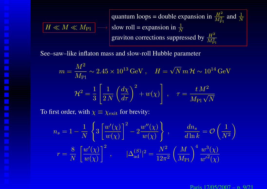
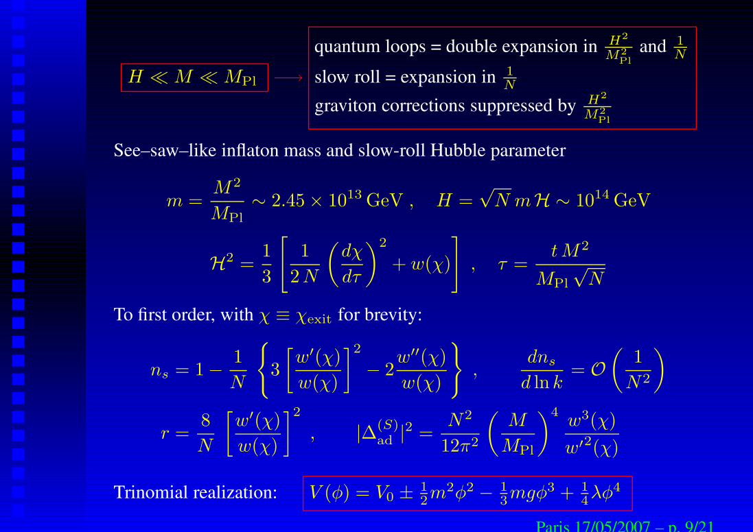
H M MPl −→quantum loops = double expansion in H2
M2
Pl
and 1N
slow roll = expansion in 1N
graviton corrections suppressed by H2
M2
Pl
Paris 17/05/2007 – p. 9/21
H M MPl −→quantum loops = double expansion in H2
M2
Pl
and 1N
slow roll = expansion in 1N
graviton corrections suppressed by H2
M2
Pl
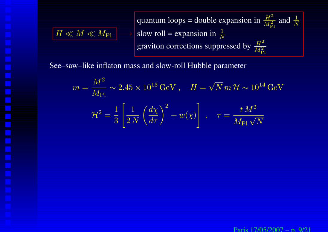
See–saw–like inflaton mass and slow-roll Hubble parameter
m =M2
MPl∼ 2.45× 10¹³ GeV , H =
√N mH ∼ 1014 GeV
Paris 17/05/2007 – p. 9/21
H M MPl −→quantum loops = double expansion in H2
M2
Pl
and 1N
slow roll = expansion in 1N
graviton corrections suppressed by H2
M2
Pl
See–saw–like inflaton mass and slow-roll Hubble parameter
m =M2
MPl∼ 2.45× 10¹³ GeV , H =
√N mH ∼ 1014 GeV
H2 =1
3
[
1
2 N
(
dχ
dτ
)2
+ w(χ)
]
, τ =t M2
MPl
√N
To first order, with χ ≡ χexit for brevity:
ns = 1− 1
N
3
[
w′(χ)
w(χ)
]2
− 2w′′(χ)
w(χ)
,dns
d ln k= O
(
1
N2
)
r =8
N
[
w′(χ)
w(χ)
]2
, |∆(S)ad |2 =
N2
12π2
(
M
MPl
)4w3(χ)
w′2(χ)
Trinomial realization: V (φ) = V0 ± 12m2φ2 − 1
3mgφ3 + 14λφ4
Paris 17/05/2007 – p. 9/21
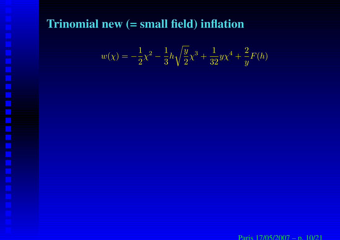
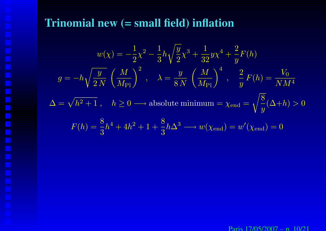
Trinomial new (= small field) inflation
w(χ) = −1
2χ2 − 1
3h
√
y
2χ3 +
1
32yχ4 +
2
yF (h)
Paris 17/05/2007 – p. 10/21
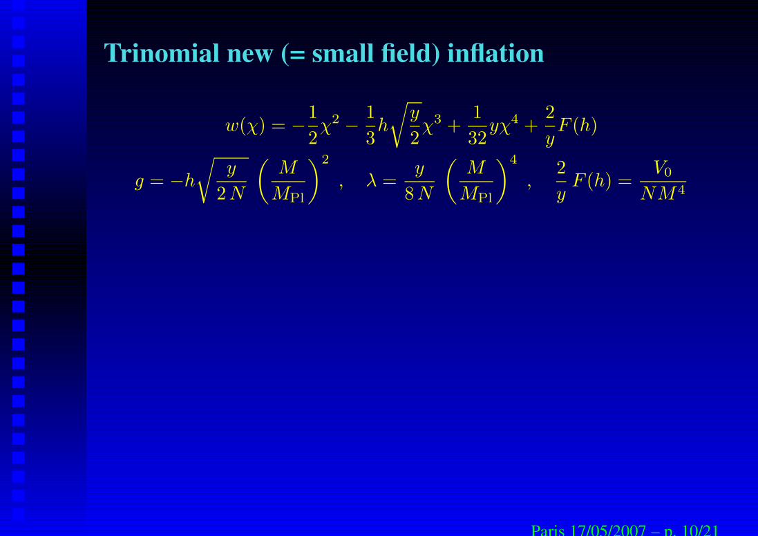
Trinomial new (= small field) inflation
w(χ) = −1
2χ2 − 1
3h
√
y
2χ3 +
1
32yχ4 +
2
yF (h)
g = −h
√
y
2 N
(
M
MPl
)2
, λ =y
8 N
(
M
MPl
)4
,2
yF (h) =
V0
NM4
Paris 17/05/2007 – p. 10/21
Trinomial new (= small field) inflation
w(χ) = −1
2χ2 − 1
3h
√
y
2χ3 +
1
32yχ4 +
2
yF (h)
g = −h
√
y
2 N
(
M
MPl
)2
, λ =y
8 N
(
M
MPl
)4
,2
yF (h) =
V0
NM4
∆ =√
h2 + 1 , h ≥ 0 −→ absolute minimum = χend =
√
8
y(∆+h) > 0
F (h) =8
3h4 + 4h2 + 1 +
8
3h∆3 −→ w(χend) = w′(χend) = 0
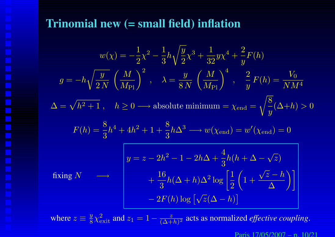
fixing N −→
y = z − 2h2 − 1− 2h∆ +4
3h(h + ∆−
√z)
+16
3h(∆ + h)∆2 log
[
1
2
(
1 +
√z − h
∆
)]
− 2F (h) log[√
z(∆− h)]
where z ≡ y8χ2
exit and z1 = 1− z(∆+h)2 acts as normalized effective coupling.
Paris 17/05/2007 – p. 10/21
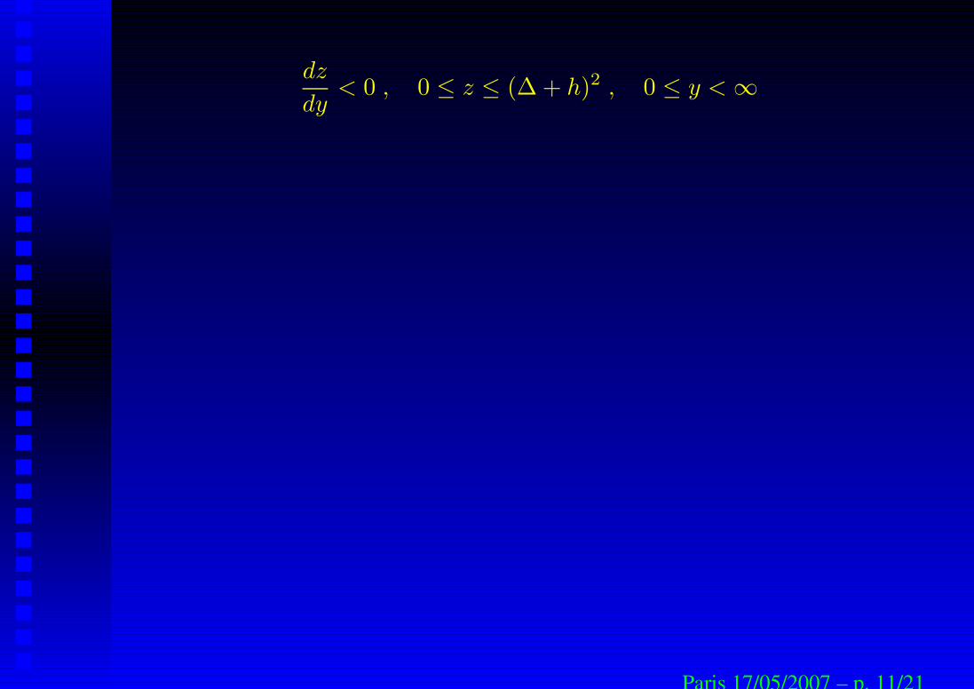
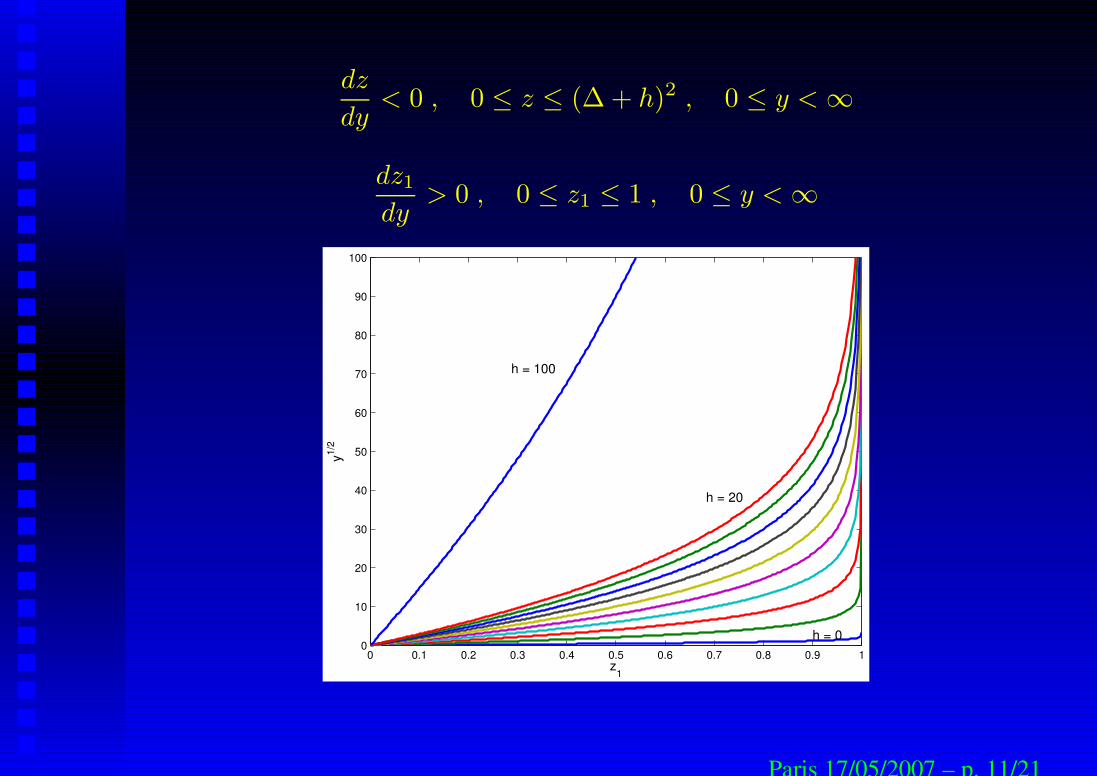
dz
dy< 0 , 0 ≤ z ≤ (∆ + h)2 , 0 ≤ y <∞
Paris 17/05/2007 – p. 11/21
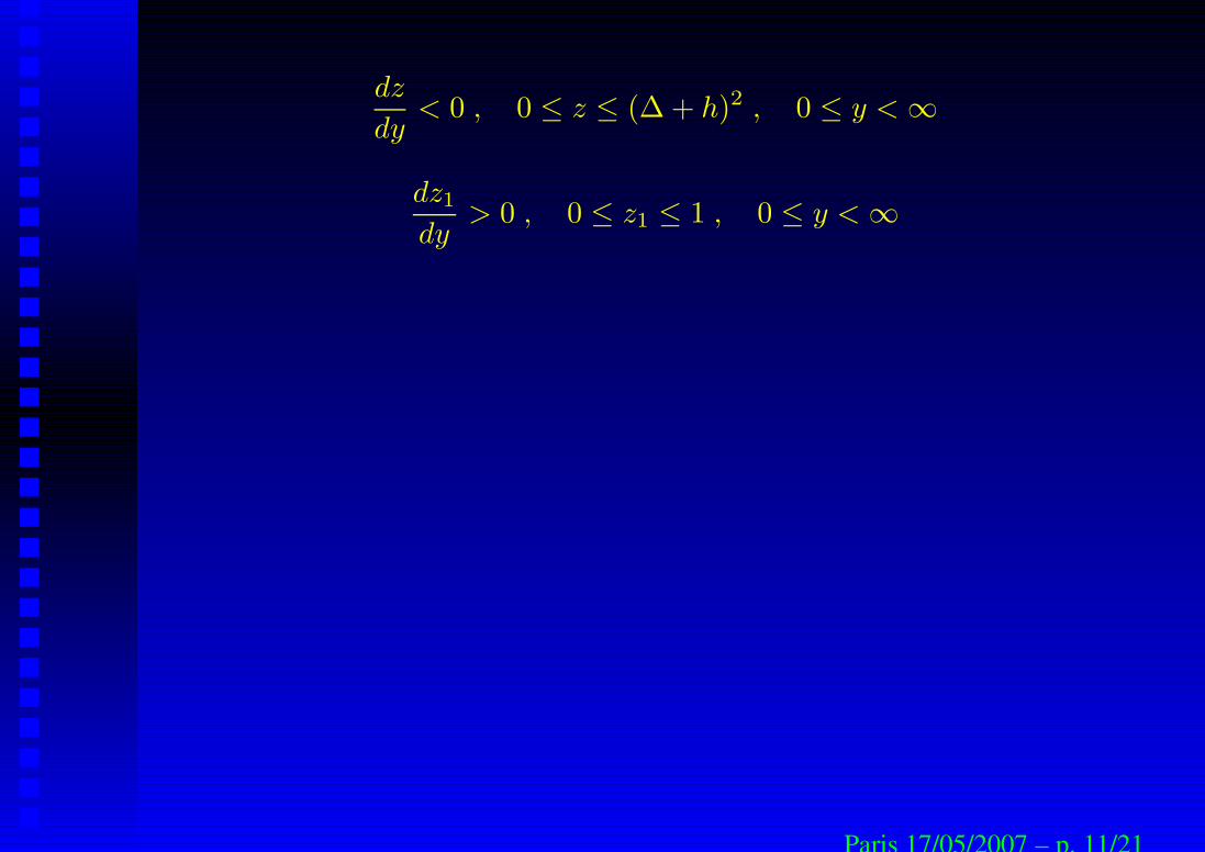
dz
dy< 0 , 0 ≤ z ≤ (∆ + h)2 , 0 ≤ y <∞
dz1
dy> 0 , 0 ≤ z1 ≤ 1 , 0 ≤ y <∞
Paris 17/05/2007 – p. 11/21
dz
dy< 0 , 0 ≤ z ≤ (∆ + h)2 , 0 ≤ y <∞
dz1
dy> 0 , 0 ≤ z1 ≤ 1 , 0 ≤ y <∞
0 0.1 0.2 0.3 0.4 0.5 0.6 0.7 0.8 0.9 10
10
20
30
40
50
60
70
80
90
100
z1
y1/2
h = 0
h = 20
h = 100
Paris 17/05/2007 – p. 11/21
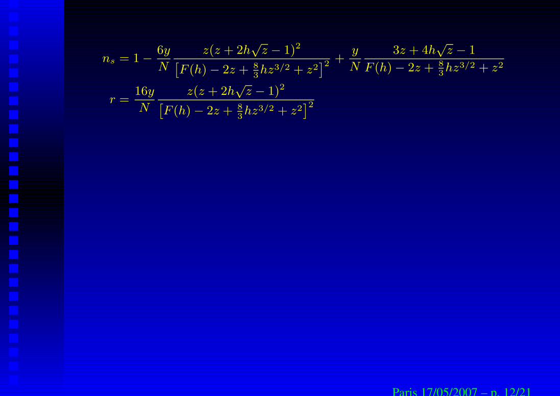
ns = 1 −6y
N
z(z + 2h√
z − 1)2ˆ
F (h) − 2z + 8
3hz3/2 + z2
˜
2+
y
N
3z + 4h√
z − 1
F (h) − 2z + 8
3hz3/2 + z2
r =16y
N
z(z + 2h√
z − 1)2ˆ
F (h) − 2z + 8
3hz3/2 + z2
˜
2
Paris 17/05/2007 – p. 12/21
ns = 1 −6y
N
z(z + 2h√
z − 1)2ˆ
F (h) − 2z + 8
3hz3/2 + z2
˜
2+
y
N
3z + 4h√
z − 1
F (h) − 2z + 8
3hz3/2 + z2
r =16y
N
z(z + 2h√
z − 1)2ˆ
F (h) − 2z + 8
3hz3/2 + z2
˜
2
0.88 0.89 0.9 0.91 0.92 0.93 0.94 0.95 0.96 0.970
0.02
0.04
0.06
0.08
0.1
0.12
0.14
0.16
ns
r
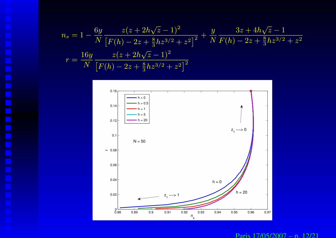
z1 −−> 1
z1 −−> 0
h = 0
h = 20
N = 50
h = 0h = 0.5h = 1h = 5h = 20
Paris 17/05/2007 – p. 12/21
ns = 1 −6y
N
z(z + 2h√
z − 1)2ˆ
F (h) − 2z + 8
3hz3/2 + z2
˜
2+
y
N
3z + 4h√
z − 1
F (h) − 2z + 8
3hz3/2 + z2
r =16y
N
z(z + 2h√
z − 1)2ˆ
F (h) − 2z + 8
3hz3/2 + z2
˜
2
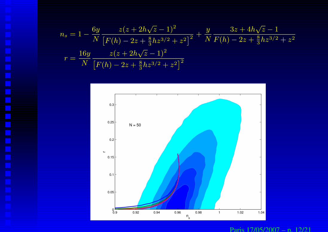
ns
r
N = 50
0.9 0.92 0.94 0.96 0.98 1 1.02 1.040
0.05
0.1
0.15
0.2
0.25
0.3
Paris 17/05/2007 – p. 12/21
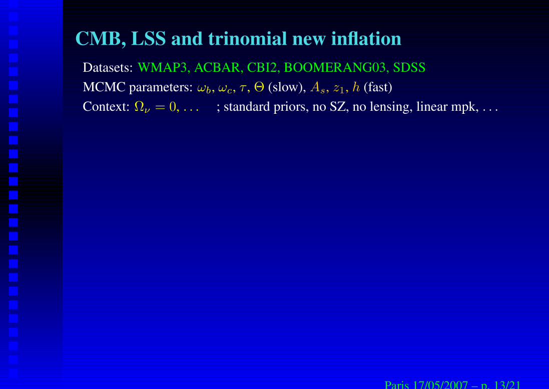
CMB, LSS and trinomial new inflationDatasets: WMAP3, ACBAR, CBI2, BOOMERANG03, SDSSMCMC parameters: ωb, ωc, τ , Θ (slow), As, z1, h (fast)Context: Ων = 0, . . . ; standard priors, no SZ, no lensing, linear mpk, . . .
Paris 17/05/2007 – p. 13/21
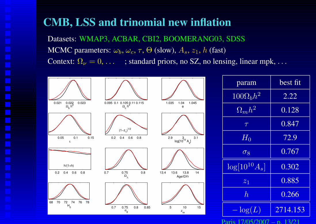
CMB, LSS and trinomial new inflationDatasets: WMAP3, ACBAR, CBI2, BOOMERANG03, SDSSMCMC parameters: ωb, ωc, τ , Θ (slow), As, z1, h (fast)Context: Ων = 0, . . . ; standard priors, no SZ, no lensing, linear mpk, . . .
0.021 0.022 0.023Ωb h2 0.095 0.1 0.105 0.11 0.115
Ωc h2 1.035 1.04 1.045
θ
0.05 0.1 0.15τ
0.2 0.4 0.6 0.8
(1−z1)1/2
2.9 3 3.1log[1010 As]
0.2 0.4 0.6 0.8
h/(1+h)
0.7 0.75 0.8ΩΛ
13.4 13.6 13.8 14Age/GYr
0.7 0.75 0.8 0.85σ8
5 10 15zre
68 70 72 74 76 78H0
param best fit
100Ωbh2 2.22
Ωmh2 0.128
τ 0.847
H0 72.9
σ8 0.767
log[1010As] 0.302
z1 0.885
h 0.266
− log(L) 2714.153Paris 17/05/2007 – p. 13/21
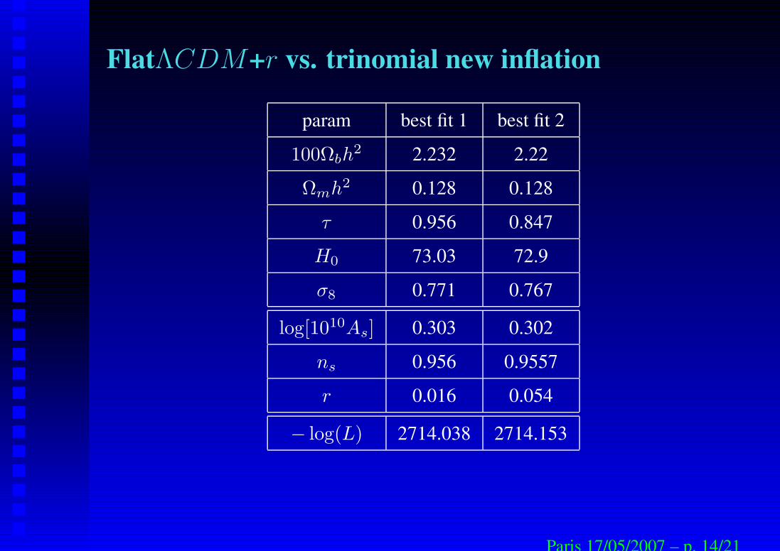
FlatΛCDM+r vs. trinomial new inflation
param best fit 1 best fit 2
100Ωbh2 2.232 2.22
Ωmh2 0.128 0.128
τ 0.956 0.847
H0 73.03 72.9
σ8 0.771 0.767
log[1010As] 0.303 0.302
ns 0.956 0.9557
r 0.016 0.054
− log(L) 2714.038 2714.153
Paris 17/05/2007 – p. 14/21

The lower bound on r
0 0.2 0.4 0.6 0.8 10
0.2
0.4
0.6
0.8
1
z1
0.94 0.945 0.95 0.955 0.96 0.9650
0.2
0.4
0.6
0.8
1
ns
0 0.05 0.1 0.150
0.2
0.4
0.6
0.8
1
r
0 5 10 15 200
0.2
0.4
0.6
0.8
1
y
Paris 17/05/2007 – p. 15/21
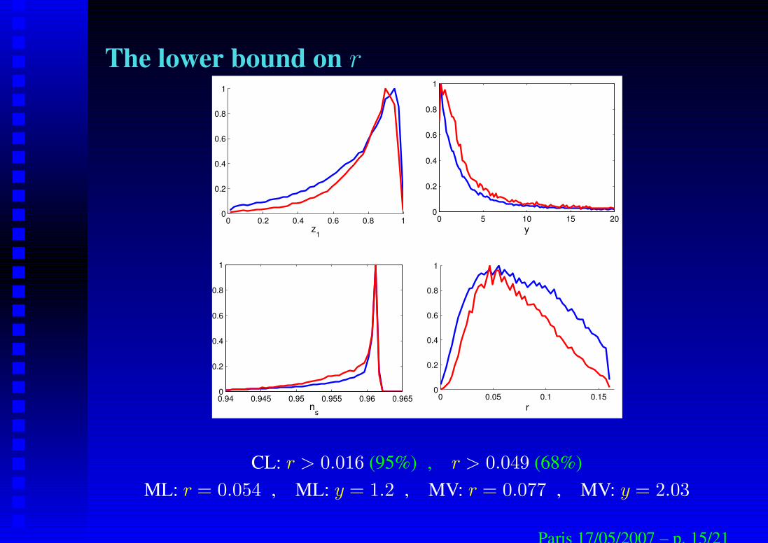
The lower bound on r
0 0.2 0.4 0.6 0.8 10
0.2
0.4
0.6
0.8
1
z1
0.94 0.945 0.95 0.955 0.96 0.9650
0.2
0.4
0.6
0.8
1
ns
0 0.05 0.1 0.150
0.2
0.4
0.6
0.8
1
r
0 5 10 15 200
0.2
0.4
0.6
0.8
1
y
CL: r > 0.016 (95%) , r > 0.049 (68%)ML: r = 0.054 , ML: y = 1.2 , MV: r = 0.077 , MV: y = 2.03
Paris 17/05/2007 – p. 15/21
Trinomial chaotic (= large field) inflation
w(χ) =1
2χ2 +
1
3h
√
y
2χ3 +
1
32yχ4 , −1 < h ≤ 0
Paris 17/05/2007 – p. 16/21
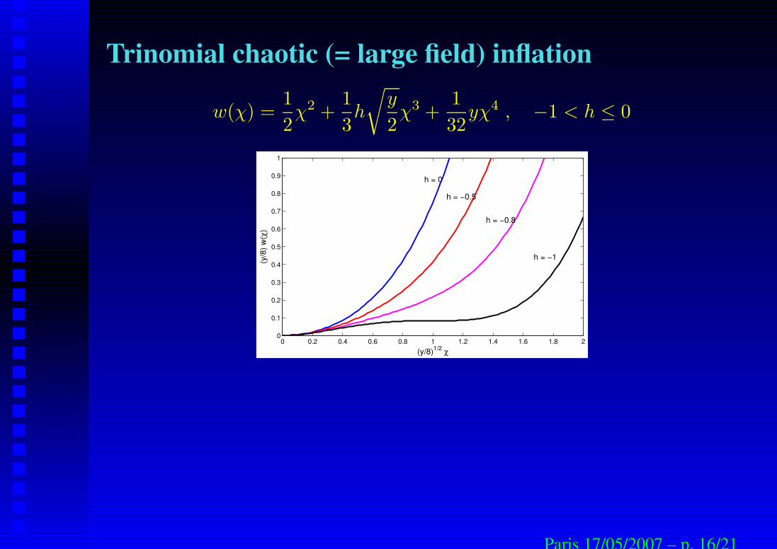
Trinomial chaotic (= large field) inflation
w(χ) =1
2χ2 +
1
3h
√
y
2χ3 +
1
32yχ4 , −1 < h ≤ 0
0 0.2 0.4 0.6 0.8 1 1.2 1.4 1.6 1.8 20
0.1
0.2
0.3
0.4
0.5
0.6
0.7
0.8
0.9
1
(y/8)1/2 χ
(y/8
) w(χ
)
h = 0
h = −0.5
h = −0.8
h = −1
Paris 17/05/2007 – p. 16/21
Trinomial chaotic (= large field) inflation
w(χ) =1
2χ2 +
1
3h
√
y
2χ3 +
1
32yχ4 , −1 < h ≤ 0
0 0.2 0.4 0.6 0.8 1 1.2 1.4 1.6 1.8 20
0.1
0.2
0.3
0.4
0.5
0.6
0.7
0.8
0.9
1
(y/8)1/2 χ
(y/8
) w(χ
)
h = 0
h = −0.5
h = −0.8
h = −1
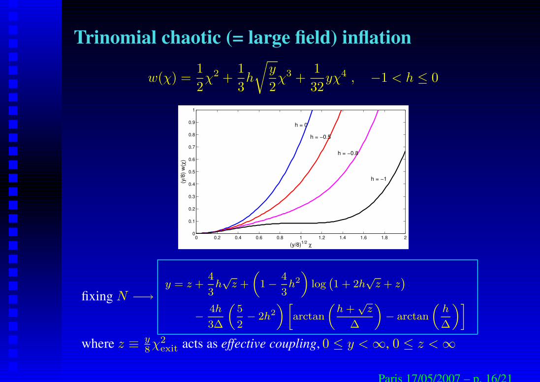
fixing N −→y = z +
4
3h√
z +
„
1 −4
3h2
«
log`
1 + 2h√
z + z´
−4h
3∆
„
5
2− 2h2
« »
arctan
„
h +√
z
∆
«
− arctan
„
h
∆
«–
where z ≡ y8χ2
exit acts as effective coupling, 0 ≤ y <∞, 0 ≤ z <∞
Paris 17/05/2007 – p. 16/21
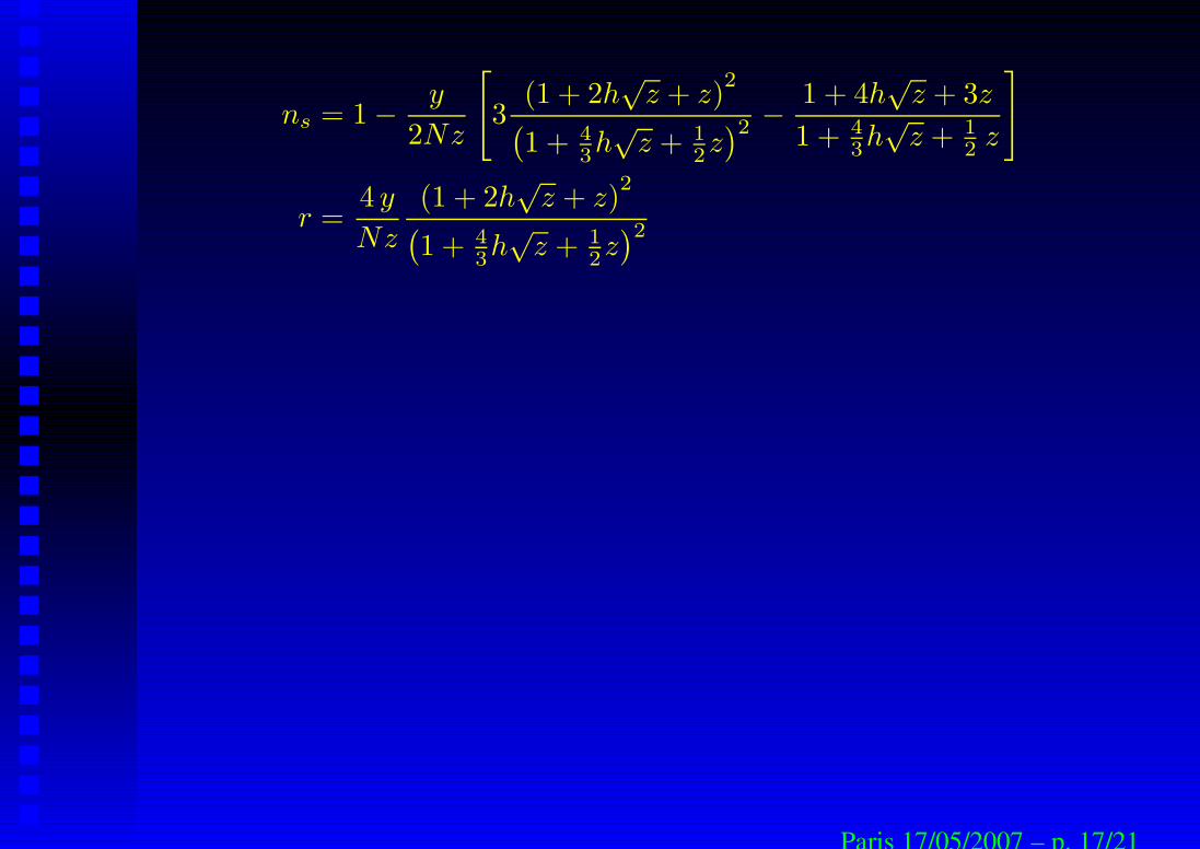
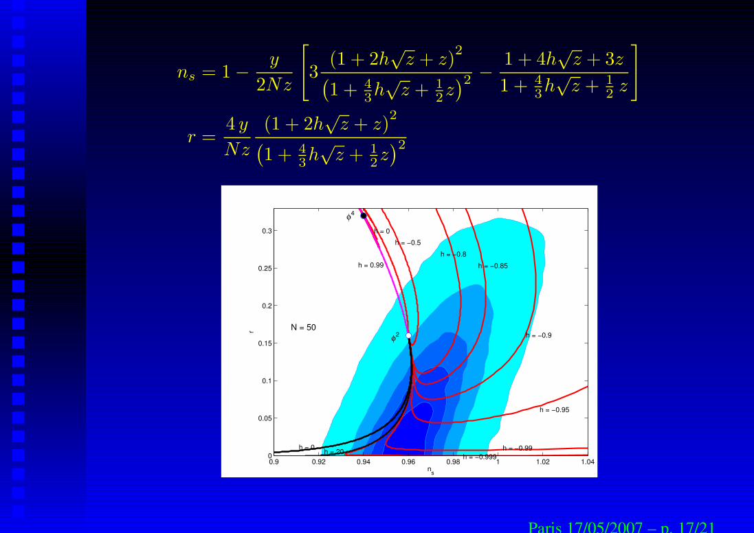
ns = 1− y
2Nz
[
3(1 + 2h
√z + z)
2
(
1 + 43h√
z + 12z)2 −
1 + 4h√
z + 3z
1 + 43h√
z + 12 z
]
r =4 y
Nz
(1 + 2h√
z + z)2
(
1 + 43h√
z + 12z)2
Paris 17/05/2007 – p. 17/21
ns = 1− y
2Nz
[
3(1 + 2h
√z + z)
2
(
1 + 43h√
z + 12z)2 −
1 + 4h√
z + 3z
1 + 43h√
z + 12 z
]
r =4 y
Nz
(1 + 2h√
z + z)2
(
1 + 43h√
z + 12z)2
ns
r
h = −0.999h = −0.99
h = −0.95
h = −0.9
h = −0.85h = −0.8
h = −0.5h = 0
h = 0.99
h = 0 h = 20
N = 50φ2
φ4
0.9 0.92 0.94 0.96 0.98 1 1.02 1.040
0.05
0.1
0.15
0.2
0.25
0.3
Paris 17/05/2007 – p. 17/21

Some limiting cases
Paris 17/05/2007 – p. 18/21
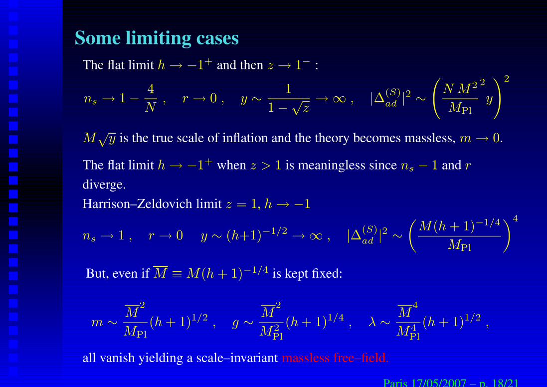
Some limiting casesThe flat limit h→ −1+ and then z → 1− :
ns → 1− 4
N, r → 0 , y ∼ 1
1−√z→∞ , |∆(S)
ad |2 ∼(
N M2
MPl
2
y
)2
M√
y is the true scale of inflation and the theory becomes massless, m→ 0.
Paris 17/05/2007 – p. 18/21
Some limiting casesThe flat limit h→ −1+ and then z → 1− :
ns → 1− 4
N, r → 0 , y ∼ 1
1−√z→∞ , |∆(S)
ad |2 ∼(
N M2
MPl
2
y
)2
M√
y is the true scale of inflation and the theory becomes massless, m→ 0.
The flat limit h→ −1+ when z > 1 is meaningless since ns − 1 and r
diverge.
Paris 17/05/2007 – p. 18/21
Some limiting casesThe flat limit h→ −1+ and then z → 1− :
ns → 1− 4
N, r → 0 , y ∼ 1
1−√z→∞ , |∆(S)
ad |2 ∼(
N M2
MPl
2
y
)2
M√
y is the true scale of inflation and the theory becomes massless, m→ 0.
The flat limit h→ −1+ when z > 1 is meaningless since ns − 1 and r
diverge.Harrison–Zeldovich limit z = 1, h→ −1
ns → 1 , r → 0 y ∼ (h+1)−1/2 →∞ , |∆(S)ad |2 ∼
(
M(h + 1)−1/4
MPl
)4
But, even if M ≡M(h + 1)−1/4 is kept fixed:
m ∼ M2
MPl(h + 1)1/2 , g ∼ M
2
M2Pl
(h + 1)1/4 , λ ∼ M4
M4Pl
(h + 1)1/2 ,
all vanish yielding a scale–invariant massless free–field.
Paris 17/05/2007 – p. 18/21
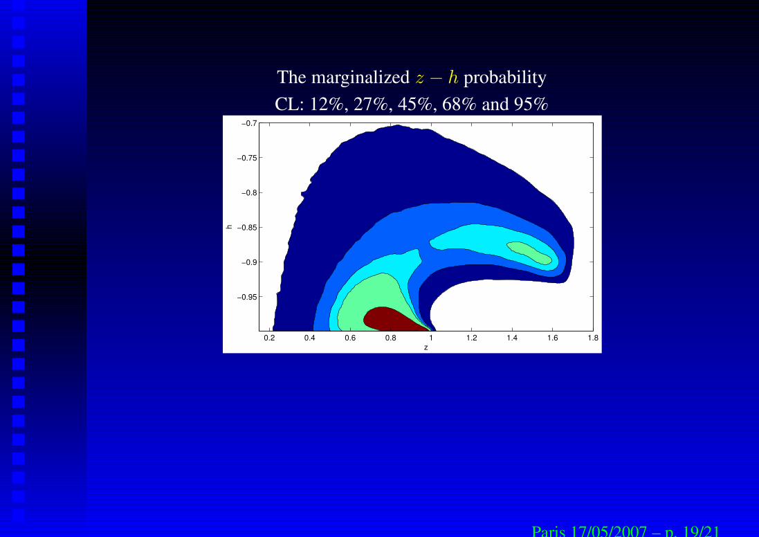
The marginalized z − h probabilityCL: 12%, 27%, 45%, 68% and 95%
z
h
0.2 0.4 0.6 0.8 1 1.2 1.4 1.6 1.8
−0.95
−0.9
−0.85
−0.8
−0.75
−0.7
Paris 17/05/2007 – p. 19/21

The marginalized z − h probabilityCL: 12%, 27%, 45%, 68% and 95%
z
h
0.2 0.4 0.6 0.8 1 1.2 1.4 1.6 1.8
−0.95
−0.9
−0.85
−0.8
−0.75
−0.7
Paris 17/05/2007 – p. 19/21

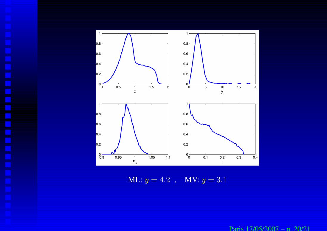
0 0.5 1 1.5 20
0.2
0.4
0.6
0.8
1
z0 5 10 15 20
0
0.2
0.4
0.6
0.8
1
y
0.9 0.95 1 1.05 1.10
0.2
0.4
0.6
0.8
1
ns0 0.1 0.2 0.3 0.4
0
0.2
0.4
0.6
0.8
1
r
ML: y = 4.2 , MV: y = 3.1
Paris 17/05/2007 – p. 20/21
0 0.5 1 1.5 20
0.2
0.4
0.6
0.8
1
z0 5 10 15 20
0
0.2
0.4
0.6
0.8
1
y
0.9 0.95 1 1.05 1.10
0.2
0.4
0.6
0.8
1
ns0 0.1 0.2 0.3 0.4
0
0.2
0.4
0.6
0.8
1
r
ML: y = 4.2 , MV: y = 3.1
Paris 17/05/2007 – p. 20/21
Summary and conclusions• Effective FT of inflation is not just phenomenology
• N plays a distingushed role
• Trinomial potentials are adequate
• Trinomial new inflation is- generically adequate (also when fully symmetric)- moderately coupled (Ginzburg–Landau safe)- provides a lower bound for r
• Trinomial chaotic inflation is- confined to a corner of parameter space- more strongly coupled- in tension with the Ginzburg–Landau picture
• Other potentials should be similarly studied (not reconstructed )
Paris 17/05/2007 – p. 21/21