Monte Carlo method for infinitely divisible random vectors ... · Monte Carlo method for infinitely divisible random vectors and Lévy processes via series representations WatRISQ

Monte Carlo method for infinitely divisible random vectors

and Lévy processes via series representations

WatRISQ Seminar at University of WaterlooSeptember 8, 2009

Junichi ImaiFaculty of Science and Technology, Keio University, JAPAN

Email:[email protected]

joint work with

Reiichiro KawaiDepartment of Mathematics, University of Leicester, United Kingdom

1

2

Purpose

The main purpose of the our research is (1)to investigate the structure of the series representation thoroughly from a simulation point of view.(2)to propose an efficient use of quasi-Monte Carlo method to the series representation of the infinitely divisible random variables.

We also discuss a Lévy process generated from a series representation of an infinitely divisible random variables and examine the efficiency of the QMC method based on the series representation.

An infinitely divisible random variable has representations of infinite sum of random variables. The existing researches in this area mainly focus on the theoretical analysis and few researches investigate a practical use of the infinite series of random variables.

• J.Imai and R.Kawai(2009), Quasi-Monte Carlo method for infinitely divisible random vectors via series representations, working paper.• J.Imai and R.Kawai(2009), Quasi-Monte Carlo method for Lévy process via series representations and its application, preworkingpaper.

Outline

1. An infinitely divisible random vector via series representation

2. Effectiveness of the QMC to the series representation

3. Numerical experiences1. moment estimation and tail probability estimation of

1. one-sided stable random variables2. gamma random variables

4. A Lévy process via series representation

5. Numerical experiences1. pricing plain vanilla options and Asian options under

1. variance gamma Lévy process2. CGMY Lévy process

1.1. An infinitely divisible random vector via series An infinitely divisible random vector via series representationrepresentation

2.2. Effectiveness of the QMC to the series representationEffectiveness of the QMC to the series representation

3.3. Numerical experiencesNumerical experiences1.1. moment estimation and tail probability estimation ofmoment estimation and tail probability estimation of

1.1. oneone--sided stable random variablessided stable random variables2.2. gamma random variablesgamma random variables

4.4. A A LLéévyvy process via series representationprocess via series representation

5.5. Numerical experiencesNumerical experiences1.1. pricing plain vanilla options and Asian options underpricing plain vanilla options and Asian options under

1.1. variance gamma variance gamma LLéévyvy processprocess2.2. CGMY CGMY LLéévyvy processprocess

3

Outline



3. Numerical experiences1. moment estimation and probability tail estimation of



5. Numerical experiences1. pricing plain vanilla and Asian options under




3.3. Numerical experiencesNumerical experiences1.1. moment estimation and probability tail estimation ofmoment estimation and probability tail estimation of



5.5. Numerical experiencesNumerical experiences1.1. pricing plain vanilla and Asian options underpricing plain vanilla and Asian options under


4

An infinite divisibility

Characteristic function of an infinitely divisible random vector X

DEFINITION: Infinite divisibility

A probability distribution F on is said to be infinitely divisible if for any integer, there exists n iid random variables such that has

distribution of F.

d

2n ≥ 1, , nY Y… 1 nY Y+ +

( ] ( ) ( )( )0

, ,12 0,1exp , , 1 , .

d

i y X i y zE e i y y Ay e i y z z dzγ ν⎡ ⎤⎡ ⎤ = − + − −⎣ ⎦ ⎢ ⎥⎣ ⎦∫ 1

where is the triplet( ), ,Aγ ν

0

,: a symmetric nonnegative-definite matrix

: Le vy measure on

d

d

A d dγ

ν

∈×

′

d-dimensional Euclidean space

5

Proposition: Infinite divisibility and Lévy processes( )

( )0

0

,Let be a Le vy process. Then, for every has an inifinite divisible distribution.

Conversely, if is an infinitely divisible distribution, then there exisits a Le vy process

such that t

t tt

t t

X t X

F X≥

≥

′

′

he distribution of is given by .tX F

Series representation via inverse Lévy measure method

Ferguson and Klass(1972) propose the inverse Lévy measure method.

[ ]( ) ( )

( ]1

0,

0, .

is an infinitely divisible random variable with Le vy measure

defined on

k kk

T dz dz

T

ν∞

=

′Γ Γ ∈ =∑ 1

Simple example: Poisson process

( ) ( ){ }( ) [ ]( )

( ) ( )( )

1

Let be the inverse of the tail as : inf 0 : . Then

: 1 0,

is an infinitely divisible random variable with Le'vy measure

defined on 0, . Note , represents arrival

u

k kk

k

H H r u h s ds r

X H T

dz h z dz

k

ν

∞

∞

=

= > <

= Γ Γ ∈

=

∞ Γ ∈

∫

∑

times of a standard Poisson process.

6

In principle, every infinitely divisible random vector has a series representation through the inverse Lévy measure method.

Example 1: stable random variable

An infinite divisible random vector X in without Gaussian component is called stable if its Lévy measure is given by

d

( ) ( ) ( ) ( )1 00,

1d

dBS

drB d r Bν σ ξ ξα−

∞= ∈

+∫ ∫ 1 BBorel sigma-field

( )1

0,2dS

α

σ −

∈where

is the stability index

: a finite positive measure on

The characteristic function of the stable random vector is given by

( ] ( ) ( )( )( ) ( )

( ) ( )

0

1

1

, ,12 0,1

2

21 2

exp , , 1 ,

exp , , 1 tan sgn , , if 1,

exp , , , ln , , if 1

d

d

d

i y X i y z

S

S

E e i y y Ay e i y z z dz

i c y i y d

i y i y y d

α παα α

ππ

γ ν

τ ξ ξ σ ξ α

τ ξ ξ ξ σ ξ α

−

−

⎡ ⎤⎡ ⎤ = − + − −⎣ ⎦ ⎢ ⎥⎣ ⎦⎧ ⎡ ⎤− − ≠⎪ ⎣ ⎦= ⎨

⎡ ⎤⎪ − + =⎣ ⎦⎩

∫

∫∫

1

Details are given in Imai and Kawai(2009)

The series representation of the stable random variable can be derived by inverse Lévy measure method.

7

( ) ( )1

1 10 01

1k kd

kX U k z z

S

α

α αα λσ

−+∞

− −−

=

⎛ ⎞⎜ ⎟= Γ − +⎜ ⎟⎝ ⎠

∑L

Series representation via “shot noise” methodBondesson(1982), Rosiński(1987)

Suppose Lévy measure can be decomposed in the form of

( ) ( ) ( )00Pr , , dB H r U B dr Bν

+∞= ∈ ∈⎡ ⎤⎣ ⎦∫ B

( ) ( )0

:

: 0, : , ,d

U

H u r H r u∞ × ∈

wherea random variable taking values in a suitable space

a function such that for each is nondecreasingU

U U

Then, an infinitely divisible random vector X generated by the triplet is identical in law to the series representation as

( )0,0,ν

( ){ }1

,k k kk

X H U c∞

=

= Γ −∑L

{ }{ }{ } ( ) ( )( ){ } { }

:

:

: : , , 1 .

wherearrival times of a standard Poisson process

sequence of iid copies of the random variable

sequence of constants defined by

and are independent

k k

k k

k k k kk

k kk k

U U

c c E H U H U

U

∈

∈

∈

∈ ∈

Γ

⎡ ⎤= Γ Γ <⎣ ⎦Γ

1

.8

• Unfortunately, the function H in the inverse Lévy measure method cannot always be given in closed form.• Alternatively, shot noise method can derive a series representation from the Lévy measure.

Example 2: gamma random variable

0, 0.a b> >where

( )0

exp 1bz

iyX iyz eE e e a dzz

−+∞⎡ ⎤⎡ ⎤ = −⎢ ⎥⎣ ⎦

⎣ ⎦∫

An infinitely divisible random variable X is called gamma if its characteristicFunction is given by

Bondesson(1982) shows that the series representation of a gamma random variable can be given by

1

k a k

k

VX e

b

+∞−Γ

=

=∑L

{ }where are arrival times of a standard Poisson process,

is a sequence of iid exponential random variables with unit mean.k

k kV

∈

Γ

9

• gamma process• variance gamma process

Note the expression is not unique.(i)Bondesson method(ii)Thinning method(iii)Rejection method

Example 3: CGMY random variable

0, 0, 0, 2C G M Y> > > <where

( ) ( ) ( )1 0 0Y G z M zdz C z e z e z dzν − − − −⎡ ⎤= < + >⎣ ⎦1 1

A CGMY random variables is characterized by Lévy measure in the form of

Carr, Geman, Madan and Yor(2002)

1 1

1 2

Y Yk k k k

k k k

Y E U VX

C V Vγ

−+∞

=

⎡ ⎤Γ⎛ ⎞= ∧ +⎢ ⎥⎜ ⎟⎝ ⎠⎢ ⎥⎣ ⎦

∑L

When then it is in a subclass of the tempered stable random vector of Rosiński(2007).

( )0,2Y ∈

{ }{ } [ ]{ }

: 0,1 ,

:

where are arrival times of a standard Poisson process:a sequence of iid exponential random variables with unit mean,

a sequence of iid uniform variables on

a sequence of iid ran

k

k k

k k

k k

E

U

V

∈

∈

∈

Γ

dom variables which take values and with equal probability,

: a suitable constantAll the random sequences are mutually independent.

G M

γ−

10CGMY process

Outline















11

Monte Carlo and quasi-Monte Carlo method

Theoretically, QMC attains a higher convergence rate than MC.QMC : O(N-1 logd N) in dimension dMC: O(N-1/2) However, the theoretical higher convergence rate of QMC is not realized for

practical sample size N, particularly for large dimension d.

Practically, the superiority of QMC lies in high uniformity of point sets in the lower dimension, which can be measured by “effective dimension”.

The accuracy of QMC is increased if the effective dimension is small enough.A couple of variance reduction methods can be utilized for decreasing or

minimizing the effective dimension.

Variance Reduction methods・Brownian Bridge：Moskowitz and Caflisch(1996), Caflisch, Morokoff and Owen(1997)

・Principal Component：Acworth, Broadie and Glasserman(1998)

・Linear Transformation：Imai and Tan(2006)

・Generalized Linear Transformation :Imai and Tan(2009)

13

ANOVA decomposition ( ) ( ){ }

( )1,2, ,

, su

u sf f f

⊆

= ∈ℜ∑x x x…

( )

( ) ( )

Function can be experessed as a sum of 2 additive functions. is a sub-function which depends on the components of in the set .

ANOVA is orthogonal;i.e., 0 .

s

u

u v

ff u

f f d for u v= ≠∫

xx

x x x

Variance ( ) ( ){ }

2 2

1,2, ,u

u sf fσ σ

⊆

= ∑…

( ) ( )[ )

( )[ )

( ) ( ){ }[ )( )

22 2

0,1 0,1

22 2

0,1

where : ,

: , : 0

s s

su u

f f d f d

f f d f

σ

σ σ ∅

⎡ ⎤= − ⎢ ⎥⎣ ⎦

= =

∫ ∫

∫

x x x x

x x

( ){ } ( )2 21,2, ,

T

.

Definition

T

T

uu d

he effective dimension of f , in the truncation sense, is the smallest integer d

such that f p fσ σ∈

≥ ⋅∑ …

[ ] ( )2Let be a function on 0,1 with 0.sf f d <∫ x x

: proportion of the variance contribution p

The effective dimension represents the number of “important” variables.It can be used for measuring the accuracy of the QMC method.

ANOVA and Effective dimensionEffective dimension can be defined through Analysis of variance(ANOVA).

14

Cumulative explanatory ratio up to dimension u can be given by

( ) ( )22 where :u

u u vv u

DCER D f

fσ

σ ⊆

= =∑

dimension dimension uu

uCER

0%0%

100%100%

Illustration of the CERIllustration of the CER

pp

Effective dimensionEffective dimension

Cumulative Explanatory Ratio(CER)

CER can capture the variance contribution of the first u dimensions.CER is used for measuring the accuracy of the QMC method.i.e., Larger CER with small u expects a success of the efficient QMC application.

15

By combining the series representation of an infinitely divisiblBy combining the series representation of an infinitely divisible random e random varibablevaribable with an with an idea of the efficient use of the QMC method, In our first paper idea of the efficient use of the QMC method, In our first paper we claim thatwe claim that

the QMC method can provide accurate estimation if we the QMC method can provide accurate estimation if we carefully assign the coordinate of the lowcarefully assign the coordinate of the low--discrepancy discrepancy sequence in simulating the infinitely divisible random variable.sequence in simulating the infinitely divisible random variable.

1. Truncation level of the series representation2. Simulation of Poisson process

Proposition

Toward an efficient simulation of the QMC

Toward efficient QMC 1: truncationSince a series representation of an infinitely indivisible random variables has a form of infinite sum we need to truncate the infinite sum up to a certain point for practical simulation.

Truncation 2: ( ) ( ){ }{ },

: ,k

k k knk n

X H U c∈ Γ ≤

= Γ −∑

kΓ

• closely related to the jump size argument in the Lévy measure• It corresponds to discarding small jumps

• difficult to implement, sorting involved

Question: How large should we take the truncation dimension N ?Examined in our numerical examples.

16

Truncation 1: ( ){ }1

: ,n

n k k kk

X H U c=

= Γ −∑

• straightforward to implement• reasonable if the function H is decreasing in

Toward the efficient QMC 2: Poisson processThe common and key building block for simulation of series representation is the sampling of the epochs of a standard Poisson process.

{ }1 2 3, , ,Γ Γ Γ … { }1 2 3

1 1 1, , ,k k kk k k

E E E= = =∑ ∑ ∑ …

L=

Gamma variable can be expressed as a sum of exponential variables.

For QMC method1.easy to use the inverse method for generating samples from exponential distribution

2.The structure naturally tends to decrease the effective dimension.

Example: sum of gamma variables

( )1 21 1 1

1n n k

k j nk k j

E nE n E E= = =

Γ = = + − + +∑ ∑∑

We can anticipate a small effective dimension if we assign the LD sequence naturally.

( )ln (0,1)j j jE U U U= − ∼ where

17

Outline















18

19

Simulation methodology

Numerical accuracy:

1. Compute relative errorto examine the effect of truncation of the series representation

2. Compute root mean square errors(RMSEs)to examine the effect of truncation of the series representation

3. Compute standard errors out of 30 iterationsto examine the accuracy of the MC and QMC

4. Compute CER(u =1,...,5) by MCto examine the efficiency of QMC

Estimation:1. Moment estimation2. Tail probability estimation

Numerical methods:1. Plain Monte Carlo

(4096 samples×30 iterations)2. RQMC(scrambled Sobol’ sequnece) + Latin Supercube sampling(LSS)

(4096 samples×30 iterations)3. Padding( QMC + MC)

( ) ( )( )

relative error Ng X g Xg X∞

∞

−=

20

1. One1. One--sided stable random variablesided stable random variable1

1

k

kX

b

αα −+∞

=

Γ⎛ ⎞= ⎜ ⎟⎝ ⎠

∑

1

1

Nk

Nk

Xb

αα −

=

Γ⎛ ⎞= ⎜ ⎟⎝ ⎠

∑truncation 1: is used where N is the truncation level.

Sato(1999)Moment estimation: ( ) ( )( ) ( )1 1

for ,1

bE X

η αη α η α

η αα η

Γ − Γ −⎛ ⎞⎡ ⎤ = ∈ −∞⎜ ⎟⎣ ⎦ Γ −⎝ ⎠

parameter values for simulation: { } { }1, 0.1,0.4,0.7 , 0.2, 4b α η α= = = −

Note is square integrable and Var is well defined.X Xη η⎡ ⎤⎣ ⎦

Tail probability estimation: [ ]lim Pr bXα

λλ λ

α↑+∞> = Samorodnitsky and Taqq(1994)

21

Moment estimation for one-sided stable random variable

The relative errors indicate that thetruncated Xn tends to X even if N is very small(N=10) for small alpha(alpha=0.1,0.4).

The comparison of the standard errors confirm QMC yields more accurate results than MC by a factor in the range of 10-200.

It is also supported by the comparison of RMSE.

The standard errors of QMC does not change against an increase of the truncation N.We conjecture that the effective dimension is small even in the high nominal dimensional problem such as N=1000.

22

CER of the moment for one-sided stable random variable

The CER is almost(round off to) 100% at the first dimension,i.e., effective dimension is 1.

These results support our claim that QMC is a good candidate for the simulation.

truncationN=1000Nominal dimension=1000

23

Tail probability estimation for one-sided stable random variable

•QMC yields more accurate estimates than MC.

• Tail probability can be accurately estimated with a small truncation level N.

24

CER of tail probability for one-sided stable random variable

The CERs are exactly 100% at the first dimension.

truncationN=1000

Samorodnitsky and Taqq(1994) discuss that the first term(k =1) of the series representation dominates the tail probability behavior.Intuitively, the first term controls the biggest jump that affect the tail probability.

1

1

Nk

Nk

Xb

αα −

=

Γ⎛ ⎞= ⎜ ⎟⎝ ⎠

∑

25

2. Gamma random variable2. Gamma random variable1

k ka

k

VX e

b

+∞ Γ−

=

=∑

1

kNka

Nk

VX e

b

Γ−

=

=∑truncation 1: is used where N is the truncation level.

Moment estimation: ( )( ) ( ) for ,

aE X b a

aη η η

η− Γ +⎡ ⎤ = ∈ − +∞⎣ ⎦ Γ

parameter values for simulation: { } { }1, 0.5,1.0,1.5 , 0.2,1b a η= = = −

Tail probability estimation: [ ] ( )11Pr for >0a z

bX z e dz

a λλ λ

+∞ − −> =Γ ∫

Note the nominal dimension is 2N.

26

Moment estimation for gamma random variable

Padding (QMC+MC)

{ } { } .W e apply QMC to the Poisson interval times while apply MC to k kk kE V

∈ ∈

1

k ka

k

VX e

b

+∞ Γ−

=

=∑truncation N=1000 nominal dimension=2000

QMC yields more accurate results than MCbut the factor is only in the range of 2-4.Similar results are confirmed even when N=50.

{ } { }We should apply QMC not only to but also to but how ?k kk kE V

∈ ∈

27

Assignment of the LD sequence in earlier dimensions

We examine the effect of the assignment of the low discrepancy sequence on the accuracy of the simulation results.

[ ] { } { }[ ] { } { }

( ), : 2

: both sequences and are generated from iid variates

: QMC solely for while MC for

Scheme I plain MC

Scheme II padding

Scheme I Prepare a -dimensional (raII QMC ndomized) LD

k kk k

k kk k

E V

E V

k k NN

∈ ∈

∈ ∈

+⎡ ⎤⎣ ⎦{ } { }

( ) : 22 1,2

sequence.

The first -dimensional poins are assgined to while the second -dimensinal points are to

Prepare a -dimensional (randomizScheme ed) LD sequence.

Every odd

IV QM

o

C

c mpo

k kk kN E N

k k

V

N∈ ∈

−⎡ ⎤⎣ ⎦{ } { }nent is assigned to while every even point is to k kk k

E V∈ ∈

Scheme III

( )1 2 3 4 5 6, , , , ,LD LD LD LD LD LD

Scheme VI

( )1 2 3 4 5 6, , , , ,LD LD LD LD LD LD

( )1 2 3, ,E E E ( )1 2 3, ,V V V ( )1 2 3, ,E E E ( )1 2 3, ,V V V

Illustration of Scheme III and Scheme VI(N=3)

The way of assignment is critical for an accuracy of the QMC.

28

Moment estimation for gamma random variable ( )0.2α = −

• QMC yields more accurate estimates than MC.• Scheme II is less accurate than Scheme III and Scheme VI. • Scheme VI is more accurate than Scheme III.

truncation N=1000Nominal dimension=2000

29

Moment estimation for gamma random variable ( )1α =

The difference is more significant in case of alpha=1.The same conclusion can be derived regardless of alpha.


30

CER of moment estimation for gamma random variable

The results of CER estimation support the fact Scheme VI is better than Scheme III.

( )( ),: ,k km nm E n VCER is # coordinates for is # coordinates for

Scheme III Scheme VI


Outline















31

32

An Infinitely divisible random variable to a Lévy process

( ){ }1

,k k kk

X H U c∞

=

= Γ −∑L

[ ]{ } ( ) { }( ) [ ]:1

1: 0, 00,, : ,t k k kk

kT TX t T H U c t t Tt∞

=

⎧ ⎫⎡ ⎤∈ = Γ − ∈⎨ ⎣ ⎦∈ ⎬⎩ ⎭∑

L

An infinitely divisible random variable

A Lévy process that are generated from the infinitely divisible random variable

{ } [ ]0,where is iid uniform variates on .k kT T

∈

represents arrival times of jumps of the Lévy process{ }k kT

∈

33

Example 1: Ornstein-Uhlenbeck process

( ),t tdX X dt z dz dtλ μ+

= − + ∫SDE:

( ) ( )0 0,

t t sttX e X e z dz dtλλ μ

+

− −−= + ∫ ∫Solution:

( )0 0, 1, , 0, 0bzX dz bae dz a bλ ν −= = = > >For simplicity, fix

( ) { }( )1

1 0,kTtt k k

k

X e e H T T tλλ∞

−

=

= Γ ∈∑Series representation:

We could estimate, for example, the first ext time with the series representation of the OU process.

34

Example 2: Variance Gamma Lévy process

Madan, Carr and Chang(1998): Option pricing under variance gamma Lévy processRibeiro and Webber(2003): use gamma subordinator, time changed gamma process

a gamma bridge is used to enhance QMCAvramidis and L’Ecuyer(2006) :generates VG process as a difference of two gamma process.

( ), ,

, , ;

t t p t n

tX Y Y

μ σ θ= −

Variance gamma process with parameter

{ } { }{ } { }{ } { }

, ,

, ,

, ,

where , are independent arrival times of a standard Poisson process

, are equences of iid exponential random variables with unit mean

, is independent sequences o

k p k pk k

k p k pk k

k p k n kk

V V

T T

∈ ∈

∈ ∈

∈∈

Γ Γ

[ ]

( ) ( )1 11 1

2 2 2 21 12 2

f iid uniform random variables on 0,

, , ,

2 2, 2 2.

p p p n n n

p n

T

a b a bν μ ν ν μ ν

μ θ σ ν θ μ θ σ ν θ

− −− −= = = =

= + + = + −

( ) ( ), ,

, ,, ,

1 1gamma process ,

k p k n

p na T k p k na Tt p k t n k

k kp n

V VY e T t Y e T t

b b

Γ Γ+∞ +∞− −

= =

= < = <∑ ∑1 1

35

Example 3: CGMY Lévy process

Carr, Geman, Madan and Yor(2002):propose CGMYRosinski(2007): derives series representation of tempered stable processes

shows that CGMY is a special case of tempered stable processes.Poirot and Tankov(2006) :Simulation of tempered stable process, including CGMY.

( ){ }, , , ; : 0tC G M Y t X t ν≥CGMY process with parameter has a Levy mesure

( ) [ ]1 1

1, 0,

2

Y Yk k k k

ktk k k

TY E U V

X tt TC

tVT V

γ−+∞

=

⎡ ⎤Γ⎛ ⎞= ∧ − ∈⎢ ⎥⎜ ⎟⎝ ⎠⎢

≤⎥⎣ ⎦

∑ 1

( ) ( ) ( )1 0 0 ,

0, 0, 0, 2.

Y G z M zdz C z e z e z dz

C G M Y

ν − − − −⎡ ⎤= < + >⎣ ⎦> ≥ ≥ <

1 1

{ }{ }{ } [ ]{ }

where is arrival times of a standard Poisson process

is a sequence of iid standard exponential random variables

is a sequence of iid uniform random variables on 0,1

is a sequence o

k k

k k

k k

k k

E

U

T

∈

∈

∈

∈

Γ

[ ]{ }

( )( ) ( )( )

1 1

f iid uniform random variables on 0,

is a sequence of iid random variables taking values , equally likely.

1 , 1,2

0, 0,1

k k

Y Y

T

V G M

C Y M G Y

Yγ

∈

− −

−

⎧ Γ − − ∈⎪= ⎨∈⎪⎩

1 1

1 2

Y Yk k k k

k k k

Y E U VX

C V Vγ

−+∞

=

⎡ ⎤Γ⎛ ⎞= ∧ +⎢ ⎥⎜ ⎟⎝ ⎠⎢ ⎥⎣ ⎦

∑L

Outline















36

37

Numerical illustrations

Numerical accuracy1. Compute standard errors out of 30 iterations

to examine the accuracy of the MC and QMC2. Compute CER(u =1,...,5) by MC

to examine the efficiency of QMC

Estimation:1. Pricing Asian call option at the money2. Pricing plain vanilla call options at the money

Numerical methods:1. Plain Monte Carlo

(4096 samples×30 iterations)2. RQMC(scrambled Sobol’ sequnce) + Latin Supercube sampling(LSS)

(4096 samples×30 iterations)

Note:Unlike using Euler method the number of nominal dimension for the LD sequencedoes not change if the number of monitoring periods increases.

38

1. Pricing option under VG 1. Pricing option under VG LLéévyvy processprocess

Parameter values are from Ribeiro and Webber(2003)

0-0.1436, 0.12136, 0.3, 1.0, 0.1, 100, 101.T r S Kμ σ θ= = = = = = =

Assignment of the LD sequence

( )1 2 3 4 5 6 7 8 9 10, , , , , , , , , ,LD LD LD LD LD LD LD LD LD LD ……

( )1, 2, 3,, , ,p p pE E E … ( )1, 2, 3,, , ,p p pV V V … ( )1, 2, 3,, , ,p p pT T T … ( )1, 2, 3,, , ,n n nE E E … ( )1, 2, 3,, , ,n n nV V V … ( )1, 2, 3,, , ,n n nT T T …

6When the number of truncation is fixed the nominal dimensions of LD sequence is .N N

For the QMC method(+) Easy to generate variates from uniform, exponential.

Note: The existing methods have to generate from complex distribution(-) The nominal dimension of the LD sequence could be huge.

The order of E,V,T is not well considered yet.

39

# truncation

# truncation

Asian call

Plain vanilla call

The effect of truncation level N

# monitoring periods for Asian =16.

• Estimation results are consistent with Ribeiro and Webber(2003).

• Both numerical results indicate that the truncated VG with finite N tends to converge rapidly, i.e., less than 30.

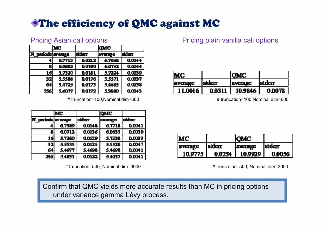
The efficiency of QMC against MC

Pricing Asian call options Pricing plain vanilla call options

# truncation=100,Nominal dim=600

# truncation=500, Nominal dim=3000 # truncation=500, Nominal dim=3000

Confirm that QMC yields more accurate results than MC in pricing options under variance gamma Lévy process.

# truncation=100,Nominal dim=600

41

CER in pricing options

Pricing Asian call options

Pricing plain vanilla call options

{ } { } { } { } { } { } { } { } { } { } { } { }, , , , , , 1,21,2 1,2 1,2 1,2 1,2

2

, , , ,k p k p k p k p k p k n kk k k k k

N

V V T T∈∈ ∈ ∈ ∈ ∈

=

Γ Γ

About 60% of the total variance can be caputured by up to the truncation level

i.e., ,

# truncation=100Nominal dim=600

# truncation=100Nominal dim=600

42

2. Pricing option under CGMY 2. Pricing option under CGMY LLéévyvy processprocess

Parameter values are from Pirot and Tankov(2006)

00.5, 2.0, 3.5, 0.5, 0.25, 0.04, 100, 100.C G M Y T r S K= = = = = = = =

Assignment of the LD sequence

( )1 2 3 4 5 6 7 8 9 10, , , , , , , , , ,LD LD LD LD LD LD LD LD LD LD ……

( )1 2 3, , ,E E E … ( )1 2 3, , ,V V V … ( )1 2 3, , ,T T T …

( )1 2 3, , ,Γ Γ Γ …

( )2 2 31 2 3, , ,E E E …

4When the number of truncation is fixed the nominal dimensions of LD sequence is .N N

6.344

6.346

6.348

6.350

6.352

6.354

6.356

6.358

6.360

6.362

6.364

0 100 200 300 400 500

3.400

3.402

3.404

3.406

3.408

3.410

3.412

3.414

3.416

0 100 200 300 400 500

43

# truncation

# truncation

Asian Put

Plain vanilla put

The effect of truncation level N

# monitoring periods for Asian =256.

• Estimation results are consistent with Poirot and Tankov(2006).

• Both numerical results indicate that the truncated CGMY with finite N tends to converge rapidly,i.e., around 40.

The efficiency of QMC against MC

Pricing Asian put options Pricing plain vanilla put options

# truncation=100, nominal dim=500

Confirm that QMC yields more accurate results than MC in pricing options under CGMY Lévy process.

# truncation=100, Nominal dim=500



45

CER in pricing optionsPricing Asian put options

Pricing plain vanilla put options



About 87% of the total variance can be captured by up to the truncation level N=2.


46

Concluding remarks

•• Series representation of an infinitely divisible random variablSeries representation of an infinitely divisible random variable is usefule is usefulfor computing moment estimates as well as tail probabilities.for computing moment estimates as well as tail probabilities.

••The estimation is accurate even if we compute with a relatively The estimation is accurate even if we compute with a relatively small small finite number of truncation level.finite number of truncation level.

•• Because of its natural structure of the series representation tBecause of its natural structure of the series representation the he effective dimension becomes very small, which enhances the effective dimension becomes very small, which enhances the efficiency of the QMC method against the MC method.efficiency of the QMC method against the MC method.

•• Numerical experiences implyNumerical experiences imply•• OneOne--sided stable random variables can be approximated by a very sided stable random variables can be approximated by a very small number of summation with its series representation.small number of summation with its series representation.

•• Gamma random variable is relatively difficult to simulate becauGamma random variable is relatively difficult to simulate because itse itinvolves two independent sequences. involves two independent sequences. But by assigning the LD sequence appropriately to each sequencBut by assigning the LD sequence appropriately to each sequence thee theefficiency of the QMC method can be significantly improved.efficiency of the QMC method can be significantly improved.

•• The idea of the series representation can be extended to a The idea of the series representation can be extended to a LLéévyvy process process by adding a sequence of jump arrival time.by adding a sequence of jump arrival time.

•• The efficiencies of the QMC method is maintained under VG and The efficiencies of the QMC method is maintained under VG and CGMY.CGMY.

Documents

Monte Carlo method for infinitely divisible random vectors ... · Monte Carlo method for infinitely divisible random vectors and Lévy processes via series representations WatRISQ