Embed Size (px)
Citation preview
Monte Carlo Modeling of Light Transport
in Multi-layered Tissues in Standard C
Lihong Wang, Ph. D.
Steven L. Jacques, Ph. D.
Laser Biology Research Laboratory
University of Texas M. D. Anderson Cancer Center
Supported by the Medical Free Electron Laser Program, the
Department of the Navy N00015-91-J-1354.
Copyright © University of Texas M. D. Anderson Cancer Center 1992

Monte Carlo Modeling of Light Transport
in Multi-layered Tissues in Standard C
Lihong Wang, Ph. D.
Steven L. Jacques, Ph. D.
Laser Biology Research Laboratory – 17
University of Texas M. D. Anderson Cancer Center
1515 Holcombe Blvd.
Houston, Texas 77030
Copyright © University of Texas
M. D. Anderson Cancer Center 1992
First printed August, 1992
Reprinted with corrections January, 1993 & November, 1995.


Abstract iii
Abstract
A Monte Carlo model of steady-state light transport in multi-layered tissue (mcml)
and the corresponding convolution program (conv) have been coded in ANSI Standard C.
The programs can therefore be executed on a variety of computers. Dynamic data
allocation is used for mcml, hence the number of tissue layers and the number of grid
elements of the grid system can be varied by users at run time as long as the total amount
of memory does not exceed what the system allows. The principle and the implementation
details of the model, and the instructions for using mcml and conv are presented here. We
have verified some of the mcml and conv computation results with those of other theories
or other investigators.

iv Acknowledgement
Acknowledgment
We would like to thank a group of people who have helped us with this package
directly or indirectly. Massoud Motamedi (University of Texas Medical Branch,
Galveston) has let us use his Sun SPARCstation 2. Scott A. Prahl (St. Vincent's Hospital,
Oregon) and Thomas J. Farrell (Hamilton Regional Cancer Center, Canada) have helped
us locate an insidious bug in the program. Craig M. Gardner (University of Texas, Austin)
provided us his Monte Carlo simulation and convolution results of a multi-layered
medium, which are compared with our results. We learned a lot from Marleen Keijzer and
Steven L. Jacques's Monte Carlo simulation program in PASCAL on Macintoshes.
Liqiong Zheng (University of Houston) has helped us greatly improve the speed of the
convolution program. They all deserve our thanks.
This work is supported by the Medical Free Electron Laser Program, the
Department of the Navy N00015-91-J-1354.

Table of Contents v
Table of Contents
Abstract ........................................................................................................... iii
Acknowledgment ............................................................................................. iv
0. Introduction ................................................................................................. 1
Part I. Description of Monte Carlo Simulation ..........................................41. The Problem and Coordinate Systems .......................................................... 4
2. Sampling Random Variables......................................................................... 7
3. Rules for Photon Propagation....................................................................... 11
3.1 Launching a photon packet ............................................................ 11
3.2 Photon's step size........................................................................... 12
3.3 Moving the photon packet ............................................................. 14
3.4 Photon absorption.......................................................................... 15
3.5 Photon scattering........................................................................... 15
3.6 Reflection or transmission at boundary........................................... 17
3.7 Reflection or transmission at interface............................................ 19
3.8 Photon termination ........................................................................ 20
4. Scored Physical Quantities ........................................................................... 22
4.1 Reflectance and transmittance ........................................................ 22
4.2 Internal photon distribution............................................................ 24
4.3 Issues regarding grid system .......................................................... 27
5. Programming mcml ...................................................................................... 32
5.1 Programming rules and conventions............................................... 32
5.2 Several constants ........................................................................... 33
5.3 Data structures and dynamic allocations......................................... 34
5.4 Flowchart of photon tracing........................................................... 38
5.5 Flow of the program mcml............................................................. 41
5.6 Multiple simulations....................................................................... 43
5.7 Timing profile of the program ........................................................ 43
6. Computation Results of mcml and Verification ............................................. 47
6.1 Total diffuse reflectance and total transmittance ............................. 47
6.2 Angularly resolved diffuse reflectance and transmittance ................ 48
6.3 Radially resolved diffuse reflectance............................................... 49
6.4 Depth resolved internal fluence ...................................................... 50
6.5 Computation times vs optical properties......................................... 52
6.6 Scored Physical Quantities of Multi-layered Tissues....................... 62

vi Table of Contents
7. Convolution for Photon Beams of Finite Size................................................67
7.1 Principles of convolution ................................................................67
7.2 Convolution over Gaussian beams ..................................................71
7.3 Convolution over circularly flat beams............................................72
7.4 Numerical solution to the convolution ............................................73
7.5 Computation results of conv and verification ..................................80
Part II. User Manual..................................................................................878. Installing mcml and conv...............................................................................87
8.1 Installing on Sun workstations........................................................87
8.2 Installing on IBM PC compatibles ..................................................88
8.3 Installing on Macintoshes ...............................................................88
8.4 Installing by Electronic Mail ...........................................................89
9. Instructions for mcml....................................................................................91
9.1 File of input data ............................................................................91
9.2 Execution.......................................................................................93
9.3 File of output data ..........................................................................95
9.4 Subset of output data .....................................................................96
9.5 Bugs of mcml .................................................................................97
10. Instructions for conv...................................................................................99
10.1 Start conv....................................................................................99
10.2 Main menu of conv......................................................................99
10.3 Command "i" of conv ..................................................................100
10.4 Command "b" of conv .................................................................100
10.5 Command "r" of conv..................................................................101
10.6 Command "e" of conv .................................................................101
10.7 Command "oo" of conv ...............................................................101
10.8 Command "oc" of conv ...............................................................103
10.9 Command "co" of conv ...............................................................104
10.10 Command "cc" of conv...............................................................105
10.11 Command "so" of conv...............................................................106
10.12 Command "sc" of conv ...............................................................107
10.13 Command "q" of conv ................................................................109
10.14 Bugs of conv ..............................................................................109
11. How to Modify mcml..................................................................................110
Appendices ................................................................................................113Appendix A. Cflow Output of the Program mcml.............................................113
Table of Contents vii
Appendix B. Source Code of the Program mcml.............................................. 117
B.1 mcml.h .......................................................................................... 117
B.2 mcmlmain.c................................................................................... 121
B.3 mcmlio.c ....................................................................................... 125
B.4 mcmlgo.c ...................................................................................... 142
B.5 mcmlnr.c ....................................................................................... 154
Appendix C. Makefile for the Program mcml................................................... 156
Appendix D. A Template of mcml Input Data File ........................................... 157
Appendix E. A Sample Output Data File of mcml............................................ 158
Appendix F. Several C Shell Scripts ................................................................ 160
F.1 conv.bat for batch processing conv ................................................ 160
F.2 p1 for pasting files of 1D arrays ..................................................... 161
Appendix G. Where to Get the Programs mcml and conv ................................ 163
Appendix H. Future Developments of the Package .......................................... 164
References .................................................................................................166Index..........................................................................................................169

Chapter 0 Introduction 1
0. Introduction
Monte Carlo simulation has been used to solve a variety of physical problems.
However, there is no succinct well-established definition. We would like to adopt the
definition by Lux et al. (1991). In all applications of the Monte Carlo method, a
stochastic model is constructed in which the expected value of a certain random variable
(or of a combination of several variables) is equivalent to the value of a physical quantity
to be determined. This expected value is then estimated by the average of multiple
independent samples representing the random variable introduced above. For the
construction of the series of independent samples, random numbers following the
distribution of the variable to be estimated are used.
Monte Carlo simulations of photon propagation offer a flexible yet rigorous
approach toward photon transport in turbid tissues. The method describes local rules of
photon propagation that are expressed, in the simplest case, as probability distributions
that describe the step size of photon movement between sites of photon-tissue interaction,
and the angles of deflection in a photon's trajectory when a scattering event occurs. The
simulation can score multiple physical quantities simultaneously. However, the method is
statistical in nature and relies on calculating the propagation of a large number of photons
by the computer. As a result, this method requires a large amount of computation time.
The number of photons required depends largely on the question being asked, the
precision needed, and the spatial resolution desired. For example, to simply learn the total
diffuse reflectance from a tissue of specified optical properties, typically about 3,000
photons can yield a useful result. To map the spatial distribution of photons, φ(r, z), in a
cylindrically symmetric problem, at least 10,000 photons are usually required to yield an
acceptable answer. To map spatial distributions in a more complex three-dimensional
problem such as a finite diameter beam irradiating a tissue with a buried blood vessel, the
required photons may exceed 100,000. The point to be remembered in these introductory
remarks is that Monte Carlo simulations are rigorous, but necessarily statistical and
therefore require significant computation time to achieve precision and resolution.
Nevertheless, the flexibility of the method makes Monte Carlo modeling a powerful tool.
Another aspect of the Monte Carlo simulations presented in this paper deserves
emphasis. The simulations described here do not treat the photon as a wave phenomenon,
and ignore such features as phase and polarization. The motivation for these simulations
2 Chapter 0 Introduction
is to predict radiant energy transport in turbid tissues. The photons are multiply scattered
by most tissues, therefore phase and polarization are quickly randomized, and play little
role in energy transport. Although the Monte Carlo simulations may be capable of
bookkeeping phase and polarization and treating wave phenomena statistically, this
manual will not consider these issues.
The Monte Carlo simulations are based on macroscopic optical properties that are
assumed to extend uniformly over small units of tissue volume. Mean free paths between
photon-tissue interaction sites typically range from 10-1000 µm, and 100 µm is a very
typical value in the visible spectrum (Cheong et al., 1990). The simulations do not treat
the details of radiant energy distribution within cells, for example.
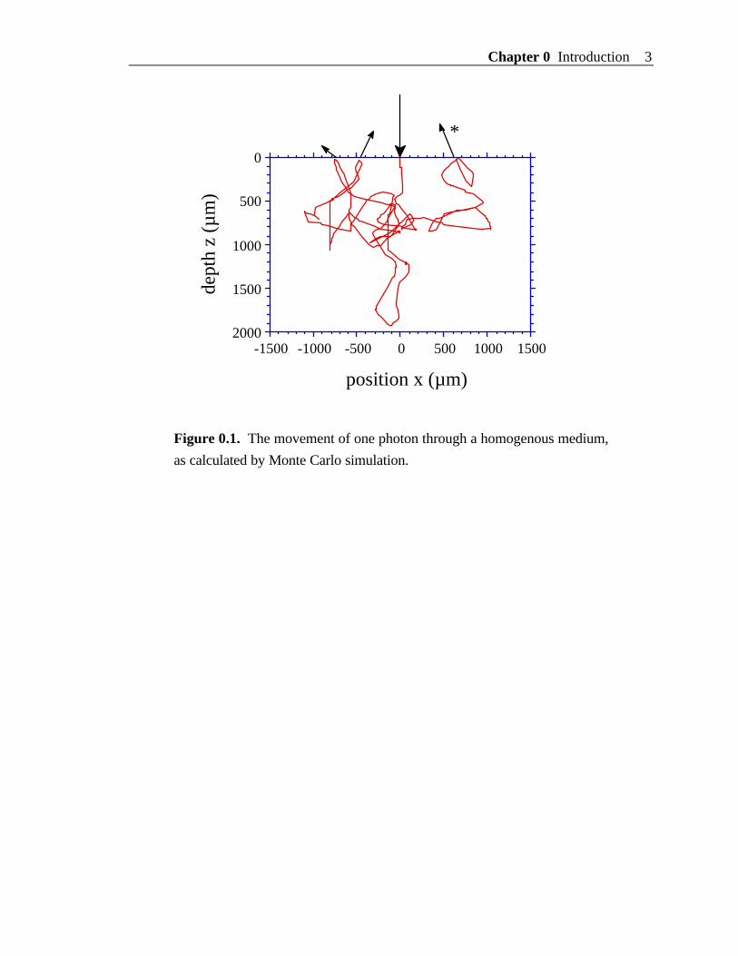
As a simple example of the Monte Carlo simulation. We would like to present a
typical trajectory of a single photon packet in Fig. 0.1. Each step between photonpositions (dots) is variable and equals –ln(ξ)/(µa + µs) where ξ is a random number and µa
and µs are the absorption and scattering coefficients, respectively (in this example, µa =
0.5 cm−1, µs = 15 cm−1, g = 0.90). The value g is the anisotropy of scattering. The
weight of the photon is decreased from an initial value of 1 as it moves through the tissue,and equals an after n steps, where a is the albedo (a = µs/(µa + µs)). When the photon
strikes the surface, a fraction of the photon weight escapes as reflectance and the
remaining weight is internally reflected and continues to propagate. Eventually, the
photon weight drops below a threshold level and the simulation for that photon is
terminated. In this example, termination occurred when the last significant fraction of
remaining photon weight escaped at the surface at the position indicated by the asterisk
(*). Many photon trajectories (104 to 106) are typically calculated to yield a statistical
description of photon distribution in the medium.
This manual is roughly divided into two major parts. Part I describes the principles
of Monte Carlo simulations of photon transport in tissues, how to realize the simulation in
ANSI Standard C, and some computation results and verifications. Part II provides users
detailed instructions of using mcml and modifying mcml to suit special need, where mcml
stands for Monte Carlo simulations for multi-layered tissues. The appendices furnish the
flow graph and the whole source code of mcml, and some other useful information.
Chapter 0 Introduction 3
2000
1500
1000
500
0
-1500 -1000
dept
h z
(µm
)
-500 0 500 1000 1500
*
position x (µm)
Figure 0.1. The movement of one photon through a homogenous medium,
as calculated by Monte Carlo simulation.
4 Chapter 1 The Problem and Coordinate Systems
Part I. Description of Monte Carlo Simulation
1. The Problem and Coordinate Systems
The Monte Carlo simulation described in this paper deals with the transport of an
infinitely narrow photon beam perpendicularly incident on a multi-layered tissue. Each
layer is infinitely wide, and is described by the following parameters: the thickness, therefractive index, the absorption coefficient µa, the scattering coefficient µs, and the
anisotropy factor g. The refractive indices of the top ambient medium (e.g., air) and
bottom ambient medium (if exists) have to be given as well. Although the real tissue can
never be infinitely wide, it can be so treated if it is much larger than the spatial extent ofthe photon distribution. The absorption coefficient µa is defined as the probability of
photon absorption per unit infinitesimal pathlength, and the scattering coefficient µs is
defined as the probability of photon scattering per unit infinitesimal pathlength. For thesimplicity of notation, the total interaction coefficient µ t, which is the sum of the
absorption coefficient µa and the scattering coefficient µs, is sometimes used.
Correspondingly, the interaction coefficient means the probability of photon interaction
per unit infinitesimal pathlength. The anisotropy g is the average of the cosine value of the
deflection angle (see Section 3.5).
Photon absorption, fluence, reflectance and transmittance are the physical
quantities to be simulated. The simulation propagates photons in three dimensions,
records photon deposition, A(x , y, z), (J/cm3 per J of delivered energy or cm−3) due to
absorption in each grid element of a spatial array, and finally calculates fluence, φ(x , y, z),
(J/cm2 per J of delivered energy or cm−2) by dividing deposition by the local absorptioncoefficient, µa in cm−1: φ(x , y, z) = A(x , y, z)/µa. Since the photon absorption and the
photon fluence can be converted back and forth through the local absorption coefficient of
the tissue, we only report the photon absorption in mcml (see Section 4.2 and Section
9.3). The photon fluence can be obtained by converting the photon absorption in another
program conv. The simulation also records the escape of photons at the top (and bottom)
surface as local reflectance (and transmittance) (cm–2sr–1) (see Section 4.1).
In this first version of mcml, we consider cylindrically symmetric tissue models.
Therefore, we chose to record photon deposition in a two-dimensional array, A(r, z)
although the photon propagation of this simulation is conducted in three-dimensions.
Chapter 1 The Problem and Coordinate Systems 5
Three coordinate systems are used in the Monte Carlo simulation at the same time.
A Cartesian coordinate system is used to trace photon packets. The origin of the
coordinate system is the photon incident point on the tissue surface, the z-axis is always
the normal of the surface pointing toward the inside of the tissue, and the xy-plane is
therefore on the tissue surface (Fig. 1.1). A cylindrical coordinate system is used to score
internal photon absorption A(r, z), where r and z are the radial and z axis coordinates of
the cylindrical coordinate system respectively. The Cartesian coordinate system and the
cylindrical coordinate system share the origin and the z axis. The r coordinate of the
cylindrical coordinate system is also used for the diffuse reflectance and totaltransmittance. They are recorded on tissue surface in Rd(r, α) and Tt(r, α) respectively,
where α is the angle between the photon exiting direction and the normal (–z axis for
reflectance and z axis for transmittance) to the tissue surfaces. A moving spherical
coordinate system, whose z axis is aligned with the photon propagation direction
dynamically, is used for sampling of the propagation direction change of a photon packet.
In this spherical coordinate system, the deflection angle θ and the azimuthal angle ψ due
to scattering are first sampled. Then, the photon direction is updated in terms of the
directional cosines in the Cartesian coordinate system (see Section 3.5).
For photon absorption, a two-dimensional homogeneous grid system is setup in z
and r directions. The grid line separations are ∆z and ∆r in z and r directions respectively.The total numbers of grid elements in z and r directions are Nz and Nr respectively. For
diffuse reflectance and transmittance, a two-dimensional homogeneous grid system is
setup in r and α directions. This grid system can share the r direction with the grid system
for photon absorption. Therefore, we only need to set up an extra one dimensional grid
system for the diffuse reflectance and transmittance in the α direction. In our simulation,
we always choose the range of α to be [0, π/2], i.e., 0 ≤ α ≤ π/2. The total number of grid
elements is Nα. Therefore the grid line separation is ∆α = π/(2 Nα).
This is an appropriate time to mention that we always use cm as the basic unit of
length throughout the simulation for consistency. For example, the thickness of each layer
and the grid line separations in r and z directions are in cm. The absorption coefficient and
scattering coefficient are in cm−1.
6 Chapter 1 The Problem and Coordinate Systems
y
z
x
Photon Beam
Layer 1
Layer N
Layer 2
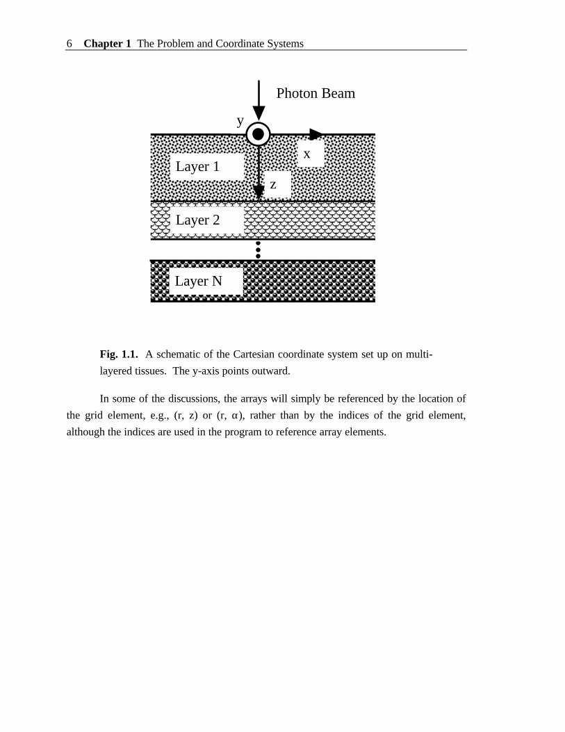
Fig. 1.1. A schematic of the Cartesian coordinate system set up on multi-
layered tissues. The y-axis points outward.
In some of the discussions, the arrays will simply be referenced by the location of
the grid element, e.g., (r, z) or (r, α), rather than by the indices of the grid element,
although the indices are used in the program to reference array elements.
Chapter 2 Sampling Random Variables 7
2. Sampling Random Variables
The Monte Carlo method, as its name implies ("throwing the dice"), relies on the
random sampling of variables from well-defined probability distributions. Several books
(Cashew et al., 1959; Lux et al., 1991; and Kalos et al., 1986) provide good references
for the principles of Monte Carlo modeling. Let us briefly review the method for sampling
random variables in a Monte Carlo simulation.
Consider a random variable χ, which is needed by the Monte Carlo simulation of
photon propagation in tissue. This variable may be the variable step size a photon will
take between photon-tissue interaction sites, or the angle of deflection a scattered photon
may experience due to a scattering event. There is a probability density function that
defines the distribution of χ over the interval (a, b). The probability density function is
normalized such that:
⌡⌠a
b p(χ) dχ = 1 (2.1)
To simulate propagation, we wish to be able to choose a value for χ repeatedly
and randomly based on a pseudo-random number generator. The computer provides a
random variable, ξ, which is uniformly distributed over the interval (0, 1). The cumulative
distribution function of this uniformly distributed random variable is:
Fξ(ξ) = 0 if ξ ≤ 0
ξ if 0 < ξ ≤ 1 1 if ξ > 1
(2.2)
To sample a generally non-uniformly distributed function p(χ), we assume there
exists a nondecreasing function χ = f(ξ) (Kalos et al., 1986), which maps ξ ∈ (0, 1) to χ ∈(a, b) (Fig. 2.1). The variable χ and variable ξ then have a one-to-one mapping. This
subsequently leads to the following equality of probabilities:
Pf(0) < χ ≤ f(ξ1) = P0 < ξ ≤ ξ1 (2.3a)
or
Pa < χ ≤ χ1 = P0 < ξ ≤ ξ1 (2.3b)
8 Chapter 2 Sampling Random Variables
According to the definition of cumulative distribution functions, Eq. 2.3b can be changed
to an equation of cumulative distribution functions:
Fχ(χ1) = Fξ(ξ1) (2.4)
Expanding the cumulative distribution function Fχ(χ1) in terms of the corresponding
probability density function for the left-hand side of Eq. 2.4 and employing Eq. 2.2 for the
right-hand side, we convert Eq. 2.4 into:
⌡⌠a
χ1
p(χ) dχ = ξ1 for ξ1 ∈ (0, 1) (2.5)
Eq. 2.5 is then used to solve for χ1 to get the function f(ξ1). If the function χ =
f(ξ) is assumed nonincreasing, a similar derivation will lead to the counterpart of Eq. 2.5
as:
⌡⌠a
χ1
p(χ) dχ = 1 – ξ1 for ξ1 ∈ (0, 1) (2.6)
However, since (1 − ξ1) and ξ1 have the same distribution, they can be interchanged.
Therefore, Eq. 2.5 and Eq. 2.6 are equivalent. In the following chapter, Eq. 2.5 will be
repeatedly invoked for sampling propagation variables.
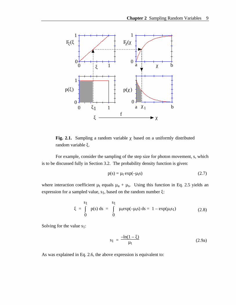
The whole sampling process can be understood from Fig. 2.1. The key to the
Monte Carlo selection of χ using ξ is to equate the probability that ξ is in the interval [0,ξ1] with the probability that χ is in the interval [a, χ1]. In Fig. 2.1, we are equating the
shaded area depicting the integral of p(χ) over [0, χ1] with the shaded area depicting the
integral p(ξ) over [0, ξ1]. Keep in mind that the total areas under the curves p(χ) and p(ξ)
each equal unity, as is appropriate for probability density functions. The result is a one-to-one mapping between the upper boundaries ξ1 and χ1 based on the equality of the shaded
areas in Fig. 2. In other words, we have equated Fχ(χ1) with Fξ(ξ1) (Eq. 2.4) which is
equivalent to Eq. 2.5. The transformation process χ1 = f(ξ1) is shown by the arrows. For
each ξ1, a χ1 is chosen such that the cumulative distribution functions for ξ1 and χ1 have
the same value. Correspondingly, the hatched areas are equal. It can also be seen in Fig.
2.1 that the monotonic function f(ξ) always exists because both cumulative distribution
functions of ξ and χ are monotonic.
Chapter 2 Sampling Random Variables 9
p(ξ)
F (ξ)
0a b
p(χ)
0
1
a bχ
0
1
0 1
ξ
0
1
0 1ξ
ξ F (χ)χ
χ1ξ1
χf
Fig. 2.1. Sampling a random variable χ based on a uniformly distributed
random variable ξ.
For example, consider the sampling of the step size for photon movement, s, which
is to be discussed fully in Section 3.2. The probability density function is given:
p(s) = µ t exp(–µ ts) (2.7)
where interaction coefficient µt equals µa + µs. Using this function in Eq. 2.5 yields an
expression for a sampled value, s1, based on the random number ξ:
ξ = ⌡⌠0
s1
p(s) ds = ⌡⌠0
s1
µ texp(–µ ts) ds = 1 – exp(µ ts1) (2.8)
Solving for the value s1:
s1 = –ln(1 – ξ)
µ t (2.9a)
As was explained in Eq. 2.6, the above expression is equivalent to:

10 Chapter 2 Sampling Random Variables
s1 = –ln(ξ)
µ t (2.9b)
Chapter 3 Rules for Photon Propagation 11
3. Rules for Photon Propagation
This chapter presents the rules that define photon propagation in the Monte Carlo
model as applied to tissues. The treatment is based upon Prahl et al. (1989) except that
we deal with a multi-layered tissue instead of a semi-infinite tissue.
3.1 Launching a photon packet
A simple variance reduction technique, implicit photon capture, is used to improve
the efficiency of the Monte Carlo simulation. This technique allows one to equivalently
propagate many photons as a packet along a particular pathway simultaneously. Each
photon packet is initially assigned a weight, W, equal to unity. The photon is injected
orthogonally into the tissue at the origin, which corresponds to a collimated arbitrarily
narrow beam of photons.
The current position of the photon is specified by the Cartesian coordinates (x, y,
z). The current photon direction is specified by a unit vector, r, which can be equivalentlydescribed by the directional cosines (µx, µy, µz):
µx = r • x
µy = r • y
µz = r • z
(3.1)
where x, y, and z are unit vectors along each axis. The photon position is initialized to (0,
0, 0,) and the directional cosines are set to (0, 0, 1). This description of photon position
and direction in a Cartesian coordinate system (Witt, 1977) turned out to be simpler than
the counterpart in a cylindrical coordinate system (Keijzer et al., 1989).
When the photon is launched, if there is a mismatched boundary at the tissue
surface, then some specular reflectance will occur. If the refractive indices of the outsidemedium and tissue are n1 and n2, respectively, then the specular reflectance, Rsp, is
specified (Born et al., 1986; Hecht, 1987):
Rsp = (n1 – n2)2
(n1 + n2)2 (3.2a)
12 Chapter 3 Rules for Photon Propagation
If the first layer is glass, which is on top of a layer of medium whose refractive index is n3,
multiple reflections and transmissions on the two boundaries of the glass layer are
considered. The specular reflectance is then computed by:
Rsp = r1 + (1–r1)2 r2 1–r1 r2
(3.2b)
where r1 and r2 are the Fresnel reflectances on the two boundaries of the glass layer:
r1 = (n1 – n2)2
(n1 + n2)2 (3.3)
r2 = (n3 – n2)2
(n3 + n2)2 (3.4)
Note that if the specular reflectance is defined as the probability of photons being
reflected without interactions with the tissue, then Eqs. 3.2a and 3.2b are not strictly
correct although they may be very good estimates of the real specular reflectance for thick
tissues. If we want to strictly distinguish the specular reflectance and the diffuse
reflectance, we can keep track of the number of interactions experienced by a photon
packet. When we score the reflectance, if the number of interactions is not zero, the
reflectance is diffuse reflectance. Otherwise, it is specular reflectance. The transmittances
can be distinguished similarly.
The photon weight is decremented by Rsp, and the specular reflectance Rsp will be
reported to the file of output data.
W = 1 – Rsp (3.5)
3.2 Photon's step size
The step size of the photon packet is calculated based on a sampling of the
probability distribution for photon's free path s ∈ [0, ∞), which means 0 ≤ s < ∞.According to the definition of interaction coefficient µ t, the probability of interaction per
unit pathlength in the interval (s', s' + ds') is:
µ t = – dPs ≥ s' Ps ≥ s' ds'
(3.6a)
Chapter 3 Rules for Photon Propagation 13
or
d(ln(Ps ≥ s')) = – µ t ds' (3.6b)
The above Eq. 3.6b can be integrated over s' in the range (0, s1), and lead to an
exponential distribution, where Ps ≥ 0 = 1 is used:
Ps ≥ s1 = exp(– µ t s1) (3.7)
Eq. 3.7 can be rearranged to yield the cumulative distribution function of free path s:
Ps < s1 = 1 – exp(– µ t s1) (3.8)
This cumulative distribution function can be assigned to the uniformly distributed random
number ξ as discussed in Chapter 2. The equation can be rearranged to provide a means
of choosing step size:
s1 = –ln(1 –ξ)
µ t (3.9a)
or substituting ξ for (1–ξ):
s1 = –ln(ξ)
µ t (3.9b)
Eq. 3.9b gives a mean free path between photon-tissue interaction sites of 1/µ t because the
statistical average of –ln(ξ) is 1, i.e., <–ln (ξ)> = 1. There is another approach to obtain
Eq. 3.9b. Employing Eq. 3.8, the probability density function of free path s is:
p(s1) = dPs < s1/ds1 = µ t exp(– µ t s1) (3.10)
p(s1) can be substituted into Eq. 2.5 to yield Eq. 3.9b, where the integration in Eq. 2.5 will
be recovered to Eq. 3.8.
In multi-layered turbid media, the photon packet may experience free flights over
multiple layers of media before an interaction occurs. In this case, the counterpart of Eq.
3.7 becomes:
Ps ≥ ssum = exp(– ∑i
µ ti si ) (3.11)
14 Chapter 3 Rules for Photon Propagation
where i is an index to a layer, the symbols µti is the interaction coefficient for the ith layer,
and si is the step size in the ith layer. The total step size ssum is:
ssum = ∑i
si (3.12)
The summation is over all the layers in which the photon packet has traveled. Eq. 3.11
does not take photon reflection and transmission at boundaries into account because they
are processed separately. The sampling equation is obtained by equating Eq. 3.11 to ξ:
∑i
µ ti si = – ln(ξ) (3.13)
As you may have seen, Eq. 3.9b is just a special case of Eq. 3.13. The sampling can be
interpreted as that the total dimensionless step size is –ln(ξ), where dimensionless step sizeis defined as the product of the dimensional step size si and the interaction coefficient µti.
Since the absorption coefficient and the scattering coefficient of a glass layer are zeros, it
does not contribute to the left hand side of Eq. 3.13. The detailed process of Eq. 3.13 will
be discussed in Section 3.6 and 3.7. Although Eq. 3.13 looks complicated, it is the
theoretical ground for the process in Section 3.6 and 3.7 which looks simpler.
From now on, we will use step size s instead of s1 or ssum for simplicity. Note that
this sampling method involves computation of a logarithm function, which is time-
consuming. This is reflected in Section 5.7. Faster methods can be used to avoid the
logarithmic computation (Ahrens et al., 1972; Marsaglia, 1961; MacLaren et al., 1964).
3.3 Moving the photon packet
Once the step size s is specified, the photon is ready to be moved in the tissue.
The position of the photon packet is updated by:
x ← x + µx s
y ← y + µy s
z ← z + µz s
(3.14)
The arrows indicate quantity substitutions. The variables on the left hand side have the
new values, and the variables on the right hand side have the old values. In an actual

Chapter 3 Rules for Photon Propagation 15
program in C, an equal sign is used for this purpose. The simplicity of Eqs. 3.14 is a
major reason for using Cartesian coordinates.
3.4 Photon absorption
Once the photon has taken a step, some attenuation of the photon weight due to
absorption by the interaction site must be calculated. A fraction of the photon's current
weight, W, will be deposited in the local grid element. The amount of deposited photon
weight, ∆W, is calculated:
∆W = W µaµ t
(3.15)
The total accumulated photon weight A(r, z) deposited in that local grid element is
updated by adding ∆W:
A(r, z) ← A(r, z) + ∆W (3.16)
The photon weight has to be updated as well by:
W ← W – ∆W (3.17)
The photon packet with the new weight W will suffer scattering at the interaction
site (discussed later). Note that the whole photon packet experiences interaction at the
end of the step, either absorption or scattering.
3.5 Photon scattering
Once the photon packet has been moved, and its weight decremented, the photon
packet is ready to be scattered. There will be a deflection angle, θ ∈ [0, π), and an
azimuthal angle, ψ ∈ [0, 2 π) to be sampled statistically. The probability distribution for
the cosine of the deflection angle, cosθ, is described by the scattering function 1) that
Henyey and Greenstein (1941) originally proposed for galactic scattering:
p(cosθ) = 1 – g2
2 (1 + g2 – 2gcosθ)3/2 (3.18)
1) Note that the scattering function we defined here is a probability density function of cosθ. It has a
difference of a constant 1/2 with the phase function defined by van de Hulst (1980).
16 Chapter 3 Rules for Photon Propagation
where the anisotropy, g, equals <cosθ> and has a value between –1 and 1. A value of 0
indicates isotropic scattering and a value near 1 indicates very forward directed scattering.
Jacques et al. (1987) determined experimentally that the Henyey-Greenstein function
described single scattering in tissue very well. Values of g range between 0.3 and 0.98 for
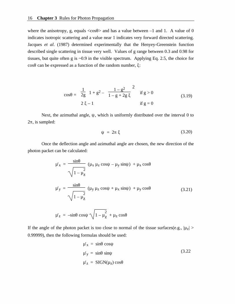
tissues, but quite often g is ~0.9 in the visible spectrum. Applying Eq. 2.5, the choice for
cosθ can be expressed as a function of the random number, ξ:
cosθ =
1
2g
1 + g2 –
1 – g2
1 – g + 2g ξ
2
if g > 0
2 ξ – 1 if g = 0
(3.19)
Next, the azimuthal angle, ψ, which is uniformly distributed over the interval 0 to
2π, is sampled:
ψ = 2π ξ (3.20)
Once the deflection angle and azimuthal angle are chosen, the new direction of the
photon packet can be calculated:
µ'x = sinθ
1 – µ
2z
(µx µz cosψ – µy sinψ) + µx cosθ
µ'y = sinθ
1 – µ
2z
(µy µz cosψ + µx sinψ) + µy cosθ
µ'z = –sinθ cosψ
1 – µ2z + µz cosθ
(3.21)
If the angle of the photon packet is too close to normal of the tissue surfaces(e.g., |µz| >
0.99999), then the following formulas should be used:
µ'x = sinθ cosψ
µ'y = sinθ sinψ
µ'z = SIGN(µz) cosθ
(3.22)
Chapter 3 Rules for Photon Propagation 17
where SIGN(µz) returns 1 when µz is positive, and it returns –1 when µz is negative.
Finally, the current photon direction is updated: µx = µ'x, µy = µ'y, µz = µ'z.
In the sampling of the two angles θ and ψ and the updating of the directional
cosines, trigonometric operations are involved. Because trigonometric operations are
computation-intensive, we should try to avoid them whenever possible. The detailed
process of the sampling can be found in the function Spin() written in the file "mcmlgo.c"
(See Appendix A and Appendix B.4).
3.6 Reflection or transmission at boundary
During a step, the photon packet may hit a boundary of the tissue, which is
between the tissue and the ambient medium, where the step size s is computed by Eq.
3.9b. For example, the photon packet may attempt to escape the tissue at the air/tissue
interface. If this is the case, then the photon packet may either escape as observed
reflectance (or transmittance if a rear boundary is also included) or be internally reflected
by the boundary. There are different methods of dealing with this problem when the step
size is large enough to hit the boundary. Let us present one of the two approaches used in
the program mcml first.
First, a foreshortened step size s1 is computed:
s1 = (z – z0)/µz if µz < 0 (z – z1)/µz if µz > 0 (3.23)
where z0 and z1 are the z coordinates of the upper and lower boundaries of the current
layer (See Fig. 1.1 for the Cartesian coordinate system). The foreshortened step size s1 is
the distance between the current photon location and the boundary in the direction of thephoton propagation. Since the photon direction is parallel with the boundary when µz is
zero, the photon will not hit the boundary. Therefore, Eq. 3.23 does not include the casewhen µz is zero. We move the photon packet s1 to the boundary with a flight free of
interactions with the tissue (see Section 3.3 for moving photon packet). The remainingstep size to be taken in the next step is updated to s ← s – s1. The photon packet will
travel the remaining step size if being internally reflected.
Second, we compute the probability of a photon packet being internally reflected,which depends on the angle of incidence, αi, onto the boundary, where αi = 0 means
orthogonal incidence. The value of αi is calculated:
18 Chapter 3 Rules for Photon Propagation
αi = cos–1(|µz|) (3.24)
Snell's law indicates the relationship between the angle of incidence, αi, the angle
of transmission, αt, and the refractive indices of the media that the photon is incident from,
ni, and transmitted to, nt:
ni sinαi = nt sinαt (3.25)
The internal reflectance, R(αi), is calculated by Fresnel's formulas (Born et al., 1986;
Hecht, 1987):
R(αi) = 12
sin2(ai –at)
sin2(ai +at) +
tan2(ai –at)
tan2(ai +at) (3.26)
which is an average of the reflectances for the two orthogonal polarization directions.
Third, we determine whether the photon is internally reflected by generating a
random number, ξ, and comparing the random number with the internal reflectance, i.e.:
If ξ ≤ R(αi), then photon is internally reflected;
If ξ > R(αi), then photon escapes the tissue(3.27)
If the photon is internally reflected, then the photon packet stays on the surfaceand its directional cosines (µx, µy, µz) must be updated by reversing the z component:
(µx, µy, µz) ← (µx, µy, –µz) (3.28)
At this point, the remaining step size has to been checked again. If it is large
enough to hit the other boundary, we should repeat the above process. If it hits a
tissue/tissue interface, we will have to process it according to the following section.
Otherwise, if the step size is small enough to fit in this layer of tissue, the photon packet
will move with the small step size. At the end of this small step, the absorption and
scattering are processed correspondingly.
On the other hand, if the photon packet escapes the tissue, the reflectance ortransmittance at the particular grid element (r, αt) must be incremented. The reflectance,
Rd(r, αt), or transmittance, Tt(r, αt), is updated by the amount of escaped photon weight,
W:
Chapter 3 Rules for Photon Propagation 19
Rd(r, αt) ← Rd(r, αt) + W if z = 0
Tt(r, αt) ← Tt(r, αt) + W if z = the bottom of the tissue.(3.29)
Since the photon has completely escaped, the tracing of this photon packet ends here. A
new photon may be launched into the tissue and traced thereafter. Note that in our
simulation, both unscattered transmittance, if any, and diffuse transmittance are scoredinto Tt(r, αt) without distinction although they could be distinguished as we discussed in
Section 3.1.
An alternative approach toward modeling internal reflectance deserves mention.
Rather than making the internal reflection of the photon packet an all-or-none event, a
partial reflection approach can be used each time a photon packet strikes the surfaceboundary. A fraction 1 – R(αi) of the current photon weight successfully escapes the
tissue, and increments the local reflectance or transmittance array, e.g., Rd(r, αt) ← Rd(r,
αt) + W (1–R(αi)). All the rest of the photon weight will be reflected, and the photon
weight is updated as W ← W R(αi).
Both approaches are available in the program mcml, and the users have the option
to use either approach depending on the physical quantities that they want to score. A
flag in the program can be changed to switch between these two approaches (see Section
5.2). The all-or-none approach is faster, but the partial reflection approach should be able
to reduce the variance of the reflectance or transmittance. It is uninvestigated how much
variance can be reduced by using the partial reflection approach.
Similar to Section 3.5, the number of trigonometric operations in Eqs. 3.24-3.26
should be minimized for the sake of computation speed. The detailed process of these
computations can be found in the function RFresnel() written in the file "mcmlgo.c" (See
Appendix A and Appendix B.4).
3.7 Reflection or transmission at interface
If a photon step size is large enough to hit a tissue/tissue interface, this step may
cross several layers of tissue. Consider a photon packet that attempts to make a step ofsize s within tissue 1 with µa1, µs1, n1, but hits an interface with tissue 2 with µa2, µs2, n2
after a foreshortened step s1. Similar to the discussion in the last section, the photon
packet is first moved to the interface without interactions, and the remaining photon stepsize to be taken in the next step is updated to s ← s – s1. Then, we have to determine
20 Chapter 3 Rules for Photon Propagation
statistically whether the photon packet should be reflected or transmitted according to the
Fresnel's formulas. If the photon packet is reflected, it is processed the same way as in the
last section. However, if the photon packet is transmitted to the next layer of tissue, it has
to continue propagation instead of being terminated. Based on Eq. 3.13, the remaining
step size has to be converted for the new tissue according to its optical properties:
s ← s µ t1µ t2
(3.30)
where µ t1 and µ t2 are the interaction coefficients for tissue 1 and tissue 2 correspondingly.
The current step size s is again checked for another boundary or interface crossing. The
above process is repeated until the step size is small enough to fit in one layer of tissue.
At the end of this small step, the absorption and scattering are processed correspondingly.
If the photon packet is in a layer of glass, the photons are moved to the boundary
of the glass layer without updating the remaining photon step size because the path length
in the glass layer does not contribute to the left hand side of Eq. 3.13. It is important to
understand that if a photon packet traverses several layers of tissues, the use of Eq. 3.9b
for the step size and the repetitive uses of Eq. 3.30 are based on Eq. 3.13.
3.8 Photon termination
After a photon packet is launched, it can be terminated naturally by reflection or
transmission out of the tissue. For a photon packet that is still propagating inside the
tissue, if the photon weight, W, has been sufficiently decremented after many steps of
interaction such that it falls below a threshold value (e.g., Wth = 0.0001), then further
propagation of the photon yields little information unless you are interested in the very late
stage of the photon propagation. However, proper termination must be executed to
ensure conservation of energy (or number of photons) without skewing the distribution of
photon deposition. A technique called roulette is used to terminate the photon packet
when W ≤ Wth. The roulette technique gives the photon packet one chance in m (e.g., m
= 10) of surviving with a weight of mW. If the photon packet does not survive the
roulette, the photon weight is reduced to zero and the photon is terminated.
W = mW if ξ ≤ 1/m0 if ξ > 1/m
(3.31)

Chapter 3 Rules for Photon Propagation 21
where ξ is the uniformly distributed pseudo-random number (see Chapter 2). This method
conserves energy yet terminates photons in an unbiased manner. The combination of
photon roulette and splitting that is contrary to roulette, may be properly used to reduce
variance (Hendricks et al., 1985).
22 Chapter 4 Scored Physical Quantities
4. Scored Physical Quantities
As we mentioned earlier, we record the photon reflectance, transmittance, and
absorption during the Monte Carlo simulation. In this chapter, we will discuss the
process of these physical quantities in detail. The dimensions of some of the quantities are
shown in square brackets at the end of their formulas.
The last cells in z and r directions require special attention. Because photons can
propagate beyond the grid system, when the photon weight is recorded into the diffuse
reflectance or transmittance array, or absorption array, the physical location may not fit
into the grid system. In this case, the last cell in the direction of the overflow is used to
collect the photon weight. Therefore, the last cell in the z and r directions do not give the
real value at the corresponding locations. However, the angle α is always within the
bound we choose for it, i.e., 0 ≤ α ≤ π/2, hence does not cause a problem in the scoring of
diffuse reflectance and transmittance.
4.1 Reflectance and transmittance
When a photon packet is launched, the specular reflectance is computed
immediately. The photon weight after the specular reflection is transmitted into the tissue.
During the simulation, some photon packets may exit the media and their weights are
accordingly scored into the diffuse reflectance array or the transmittance array depending
on where the photon packet exits. After tracing multiple photon packets (N), we havetwo scored arrays Rd(r, α) and Tt(r, α) for diffuse reflectance and transmittance
respectively. They are internally represented by Rd-rα[ir, iα] and Tt-rα[ir, iα] respectively
in the program. The coordinates of the center of a grid element are computed by:
r = (ir + 0.5) ∆r [cm] (4.1)
α = (iα + 0.5) ∆α [rad] (4.2)
where ir and iα are the indices for r and α. The raw data give the total photon weight in
each grid element in the two-dimensional grid system. To get the total photon weight in
the grid elements in each direction of the two-dimensional grid system, we sum the 2D
arrays in the other dimension:
Chapter 4 Scored Physical Quantities 23
Rd-r[ir] = ∑iα=0
Nα–1 Rd-rα [ir, iα] (4.3)
Rd-α[iα] = ∑ir=0
Nr–1 Rd-rα [ir, iα] (4.4)
Tt-r[ir] = ∑iα=0
Nα–1 Tt-rα [ir, iα] (4.5)
Tt-α[iα] = ∑ir=0
Nr–1 Tt-rα [ir, iα] (4.6)
To get the total diffuse reflectance and transmittance, we sum the 1D arrays again:
Rd = ∑ir=0
Nr–1 Rd-r [ir] (4.7)
Tt = ∑ir=0
Nr–1 Tt-r [ir] (4.8)
All these arrays give the total photon weight per grid element, based on N initialphoton packets with weight unity. To convert Rd-rα[ir, iα] and Tt-rα[ir, iα] into photon
probability per unit area perpendicular to the photon direction per solid angle, they are
divided by the projection of the annular area onto a plane perpendicular to the photon
exiting direction (∆a cosα), the solid angle (∆Ω) spanned by a grid line separation in the αdirection around an annular ring, and the total number of photon packets (N):
Rd-rα[ir, iα] ← Rd-rα[ir, iα] / (∆α cosα ∆Ω N) [cm–2 sr–1] (4.9)
Tt-rα[ir, iα] ← Tt-rα[ir, iα] / (∆α cosα ∆Ω N) [cm–2 sr–1] (4.10)
24 Chapter 4 Scored Physical Quantities
where
∆α = 2 π r ∆r = 2 π (ir + 0.5) (∆r)2 [cm2] (4.11)
∆Ω = 4 π sinα sin(∆α/2) = 4 π sin[(iα + 0.5) ∆α] sin(∆α/2) [sr] (4.12)
where r and α are computed from Eq. 4.1 and Eq. 4.2 respectively. The radially resolveddiffuse reflectance Rd-r[ir] and total transmittance Tt-r[ir] are divided by the area of the
annular ring (∆a) and the total number of photon packets (N) to convert them into photon
probability per unit area:
Rd-r[ir] ← Rd-r[ir] / (∆α N) [cm–2] (4.13)
Tt-r[ir] ← Tt-r[ir] / (∆α N) [cm–2] (4.14)
The angularly resolved diffuse reflectance Rd-α[iα] and total transmittance Tt-α[iα] are
divided by the solid angle (∆Ω) and the total number of photon packets (N) to convert
them into photon probability per unit solid angle:
Rd-α[iα] ← Rd-α[iα] / (∆Ω N) [sr–1] (4.15)
Tt-α[iα] ← Tt-α[iα] / (∆Ω N) [sr–1] (4.16)
The total diffuse reflectance and transmittance are divided by the total number of photon
packets (N) to get the probabilities:
Rd ← Rd / N [–] (4.17)
Tt ← Tt / N [–] (4.18)
where [–] means dimensionless units.
4.2 Internal photon distribution
During the simulation, the absorbed photon weight is scored into the absorptionarray A(r, z). A(r, z) is internally represented by a 2D array Arz[ir, iz], where ir and iz are
the indices for grid elements in r and z directions. The coordinates of the center of a grid
element can be computed by Eq. 4.1 and the following:
Chapter 4 Scored Physical Quantities 25
z = (iz + 0.5) ∆z (4.19)
The raw data Arz[ir, iz] give the total photon weight in each grid element in the two-
dimensional grid system. To get the total photon weight in each grid element in the z
direction, we sum the 2D array in the r direction:
Az[iz] = ∑ir=0
Nr–1 Arz [ir, iz] (4.20)
The total photon weight absorbed in each layer Al[layer] and the total photon weight
absorbed in the tissue A can be computed from Az[iz]:
Al[layer] = ∑iz in layer
Az [iz] (4.21)
A = ∑iz=0
Nz–1 Az [iz] (4.22)
where the summation range "iz in layer" includes all iz's that lead to a z coordinate in the
layer. Then, these quantities are scaled properly to get the densities:
Arz[ir, iz] ← Arz[ir, iz] / (∆α ∆z N) [cm–3] (4.23)
Az[iz] ← Az[iz] / (∆z N) [cm–1] (4.24)
Al[layer] ← Al[layer] / N [–] (4.25)
A ← A / N [–] (4.26)
The quantity A gives the photon probability of absorption by the tissue. The 1D arrayAl[layer] gives the photon probability of absorption in each layer. At this point, Arz[ir, iz]
gives the absorbed photon probability density (cm−3), and can be converted into photonfluence, φrz, (cm−2) by dividing it by the absorption coefficient µa (cm−1) of the layer
where the current location resides:
26 Chapter 4 Scored Physical Quantities
φrz[ir, iz] = Arz[ir, iz] / µa [cm–2] (4.27)
The 1D array Az[iz] gives the photon probability per unit length in the z direction (cm−1).
It can also be divided by the absorption coefficient µa (cm−1) to yield a dimensionless
quantity φz[iz]:
φz[iz] = Az[iz] / µa [–] (4.28)
This quantity may seem hard to understand or redundant at first glance. However, the
summation of the raw data in Eq. 4.20 is equivalent to the convolution for an infinitely
wide flat beam in Eq. 7.15 to be discussed in Chapter 7. The equivalence can be shown asfollows. According to Eqs. 4.20, 4.23 and 4.24, the final converted Az[iz] and Arz[ir, iz]
have the following relation:
Az[iz] = ∑ir=0
Nr–1 Arz [ir, iz] ∆α(ir) (4.29)
where ∆a(ir) is computed in Eq. 4.11, but we stress that it is a function of ir in Eq. 4.29.
Employing Eqs. 4.27 and 4.28, Eq. 4.29 can be converted to:
φz[iz] = ∑ir=0
Nr–1 frz [ir, iz] ∆α(ir) (4.30)
This is a numerical solution of the following integral:
φz(z) = ⌡⌠ 0
∞ frz(r, z) 2 π r dr (4.31)
Eq. 4.31 is essentially Eq. 7.15 for an infinitely wide flat beam with a difference of
constant S, where S is the power density of the infinitely wide flat beam. The equivalencebetween Eq. 4.31 and Eq. 7.15 can be seen after substituting φz(z) for F(r, z), φrz(r, z) for
G(r'', z), and r for r''. Therefore, φz[iz] gives the fluence for an infinitely wide flat beam
with a difference of a constant which is the power density S.
The program mcml will only report Arz[ir, iz] and Az[iz] instead of φrz[ir, iz] and
φz[iz]. The program conv will be set up to convert Arz[ir, iz] and Az[iz] into φrz[ir, iz] and
φz[iz].

Chapter 4 Scored Physical Quantities 27
4.3 Issues regarding grid system
In our Monte Carlo simulation, we always set up a grid system. The computation
results will be limited by the finite grid size. This section will discuss what is the best that
one can do.
Position of average value for each grid element
The simulation provides the average value of the scored physical quantities in each
grid element. Now, the question is at what position should that averaged value be
assigned? One can argue that there is no best point because the exact answer to the
physical quantities is unknown. However, under linear approximations of the physical
quantities in each grid element, we can find the best point for each grid point. The linear
approximations can be justified for small grid size in most cases because the higher order
terms are considerably less than the linear term. Some special occasions will be discussed
subsequently.
Let us discuss the grid system in the r direction first because r is the variable over
which the convolution for photon beams of finite size will be implemented (see Chapter 7).
The grid system in the r direction uses ∆r as the grid separation with a total of N grid
elements. The index to each grid element is denoted by n. The center of each gridelement is denoted by rn:
rn = (n + 0.5) ∆r (4.32)
As we have mentioned, the Monte Carlo simulation actually approximates the
average of the physical quantity Y(r) in each grid element, where Y(r) can be the diffusereflectance, diffuse transmittance, and internal fluence Arz(r, z) for a particualr z value.
<Y(r)> = 1
2 π rn ∆r ⌡
⌠
rn – ∆r/2
rn + ∆r/2
Y(r) 2 π r dr (4.33)
where 2 π rn ∆r is the area of the ring or the circle when n = 0.
If Y(r) in each grid element is approximated linearly, we can prove that there existsa best point rb to satisfy:
28 Chapter 4 Scored Physical Quantities
<Y(r)> = Y(rb) (4.34)
where
rb = rn + ∆r
12 rn ∆r (4.35)
Proof: Y(r) is approximated by a Taylor series about rb expanded to the first order:
Y(r) = Y(rb) + (r – rb) Y'(rb) (4.36)
Substituting Eq. 4.36 into Eq. 4.33 yields:
<Y(r)> = 1
2 π rn ∆r ⌡
⌠
rn – ∆r/2
rn + ∆r/2
[Y(rb) + (r – rb) Y'(rb)] 2 π r dr
= Y(rb)
2 π rn ∆r ⌡
⌠
rn – ∆r/2
rn + ∆r/2
2 π r dr + Y'(rb)
2 π rn ∆r ⌡
⌠
rn – ∆r/2
rn + ∆r/2
(r – rb) 2 π r dr
= Y(rb)
2 π rn ∆r [π r2]
rn + ∆r/2
rn – ∆r/2 +
Y'(rb) 2 π rn ∆r
(π/3) [2 r3 – 3 rb r2] rn + ∆r/2
rn – ∆r/2
= Y(rb)
2 π rn ∆r [2 π rn ∆r] +
Y'(rb) 2 π rn ∆r
(π/3) [2 ∆r (3 rn2 + (∆r)2
4 – 3 rb rn)]
= Y(rb) + Y'(rb) [rn + (∆r)2
12 rn – rb]
or
<Y(r)> = Y(rb) + Y'(rb) [rn + (∆r)2
12 rn – rb] (4.37)
If we set the term in the square bracket in Eq. 4.37 to zero, and solve for rb, we obtain:

Chapter 4 Scored Physical Quantities 29
rb = rn + (∆r)2
12 rn (4.38a)
and Eq. 4.37 becomes:
<Y(r)> = Y(rb) (4.39)
Eq. 4.38a can be reformulated:
rb = rn + ∆r
12 rn ∆r (4.38b)
Q.E.D.
We can substitute Eq. 4.32 into the second term of Eq. 4.38b:
rb = [(n + 0.5) + 1
12 (n + 0.5) ] ∆r (4.38c)
When n = 0, rb = [0.5 + 16 ] ∆r =
23 ∆r
When n = 1, rb = [1.5 + 118 ] ∆r ≈ 1.556 ∆r
When n = 2, rb = [2.5 + 130 ] ∆r ≈ 2.533 ∆r
When n = 3, rb = [3.5 + 142 ] ∆r ≈ 3.524 ∆r
When n = 4, rb = [4.5 + 154 ] ∆r ≈ 4.519 ∆r
...
It is observed that the best point deviates from the center of each grid element, and
the smaller the index to the grid box, the larger the deviation. As the index n becomes
large, the best point approaches the center of the grid element. This behavior is due to the
2 π r factor in Eq. 4.33. A similar factor does not exist for the z direction, and the best
points for the z direction should be the centers of each grid element.
30 Chapter 4 Scored Physical Quantities
The computation results of a Monte Carlo simulation with a selected grid system
always have finite precision which is fundamentally limited by the finite grid size. The
above theorem only gives the points where the function values are best represented by the
simulated results.
Effects of the first photon-tissue interaction
The above theorem assumed differentiability of Y(r), where Y(r) can represent thediffuse reflectance Rd(r), the diffuse transmittance Td(r), and the internal fluence φrz(r, z)
at a particular z value. This assumption should hold for the diffuse reflectance and the
diffuse transmittance. However, for the internal fluence, the on-z-axis fluence is a delta
function for an impulse response (responses to an infinitely narrow photon beam).Therefore, you cannot assume the differentiability of the function φrz(r, z) at r equal zero,
i.e., φrz(r=0, z). The best solution to this problem has been provided by Gardner et al.
(1992b). They keep track of the first photon interactions with the medium, which are
always on the z-axis, separately from the rest of the interactions. Therefore, the functionφrz(r, z) will not include the first photon-tissue interaction which yield a delta function.
This approach ensures a differentiable φrz(r, z) at r equal zero besides its better accuracy.
In the current version (version 1.0) of mcml, Gardner et al.'s approach is not yet
implemented although we intend to add this in the later version. However, the result from
mcml will still be correct within the spatial resolution of the grid size in the r direction.
Although nobody will use Monte Carlo to simulate the responses in an absorption-only
semi-infinite medium, let us use this simple example to illustrate what we mean. In this
case, Gardner et al.'s approach will yield an exponentially decaying response on the z axis
which is a delta function of r. The version 1.0 of mcml will yield the same exponentially
decaying response in the first grid elements which is not a delta function because of the
finite volume of the grid elements. However, as the grid separation ∆r is made sufficiently
small, the result approaches Gardner et al.'s.
So far the discussion has nothing to do with convolution for photon beams of finite
size which will be discussed in Chapter 7. According to Gardner et al. (1992b), the error
in the convolution caused by not scoring the first interactions separately will be small for
Gaussian beams whose radius is at least three times larger than the grid separation ∆r. As
we will discuss in Section 7.4, our extended trapezoidal integration, instead of integrating
over the original grid points, in the convolution program conv should further decrease the
error. Of course, when the on-z-axis interactions are considered separately, our

Chapter 4 Scored Physical Quantities 31
convolution program conv is not subject to this limitation on the radius of the Gaussian
beam. In contrast, if the integration is approximated by computing the integrand over the
original grid points, the radius of the photon beam should still be large enough to yield
reasonable integration accuracy.
Since this theorem is a late development, it has not been implemented in the
programs (mcml and conv) yet. We plan to implement it in the next release (see Appendix
H).

32 Chapter 5 Programming mcml
5. Programming mcml
The simulation is written in ANSI Standard C (Plauger et al., 1989, Kelley et al.,
1990), which makes it possible to execute the program on any computers that support
ANSI Standard C. So far, the program has been successfully tested on Macintosh, IBM
PC compatibles, Sun SPARCstation 2, IBM RISC/6000 POWERstation 320, and Silicon
Graphics IRIS workstation. This chapter mainly describes several rules, the important
constants and the data structures used in the program, the algorithm to trace photon
packets, flow of the program, and the timing profile of the program. Prior knowledge of
C is assumed to fully understand this chapter. The flow of the program is listed in detail in
Appendix A. The complete source code is listed in Appendix B file by file. In Appendix
C, we have provided a make file used by make utilities on UNIX machines. Appendix D
and E are a template of input data file and a sample output data file respectively.
Appendix F gives several C Shell scripts for UNIX users. The information needed to
obtain the program is detailed in Appendix G.
5.1 Programming rules and conventions
When we write this program, we have followed the following rules and
conventions:
1. Conform to ANSI Standard C so that the program can be executed on a variety of
computers.
2. Avoid global variables whenever possible. This program has not defined any
global variables so far.
3. Avoid hard limits on the program. For example, we removed the limits on the
number of array elements by dynamic allocation at run time. This means that the
program can accept any number of layers or gridlines as long as the memory
permits.
4. Preprocessor names are all capital letters, e.g.,
#define PREPROCESSORS
5. For global variables, function names, or data types, first letter of each word is
capital, and words are connected without underscores, e.g.,
Chapter 5 Programming mcml 33
short GlobalVar;
6. For dummy variables, first letter of each word is capital, and words are connected
by underscores, e.g.,
void NiceFunction(char Dummy_Var);
7. Local variables are all lower cases, and words are connected by underscores, e.g.,
short local_var;
5.2 Several constants
There are several important constants defined in the header file mcml.h or the
source files mcmlmain.c and mcmlgo.c. They are listed in Table 5.1, and may be altered
according to your special need.
The constant STRLEN is used in the program to define string length. WEIGHT is the
threshold photon weight, below which the photon packet will go through a roulette. This
photon packet with small weight W has a chance of CHANCE to survive with a new weight
of W/CHANCE. COSZERO and COS90D are used for the computation of reflection with
Fresnel's formulas, and for the computation of new photon directional cosines. When
|cosα| > COSZERO, α is considered very close to 0 or 180o. When |cosα| < COS90D, α is
considered very close to 90o.
When THINKCPROFILER is 1, the profiler of THINK C compiler (Symantec, 1991)
on Macintosh can be used to monitor the timing profile of the program regarding each
function (see Section 5.7). When GNUCC is 1, the code can be compiled with GNU C
compiler (gcc) from the Free Software Foundation, which does not support several
functions such as difftime() although being claimed to conform to ANSI C standards.
Therefore, the timing modules in the program will not work when GNUCC is 1, although the
program will otherwise operate normally. When STANDARDTEST is 1, the random number
generator will generate a fixed sequence of random numbers after being fed a fixed seed.
This feature is used to debug the program. STANDARDTEST should be set to 0 normally,
which makes the random number generator use the current time as the seed. When
PARTIALREFLECTION is set to 0, the all-or-none simulation mechanism of photon internal
reflection at a boundary (e.g., air/tissue boundary) described in Section 3.6 is used, where
the photon packet is either totally reflected or totally transmitted determined by the
comparison of the Fresnel reflectance and a random number. Otherwise when
PARTIALREFLECTION is set to 1, the photon packet will be partially reflected and
34 Chapter 5 Programming mcml
transmitted. Normally we set PARTIALREFLECTION to 0 because the all-or-none simulation
is faster.
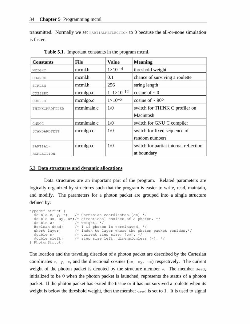
Table 5.1. Important constants in the program mcml.
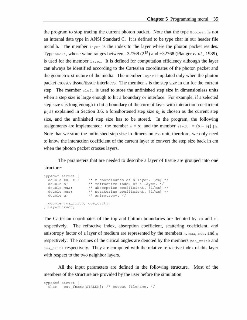
5.3 Data structures and dynamic allocations
Data structures are an important part of the program. Related parameters are
logically organized by structures such that the program is easier to write, read, maintain,
and modify. The parameters for a photon packet are grouped into a single structure
defined by:
typedef struct double x, y, z; /* Cartesian coordinates.[cm] */ double ux, uy, uz;/* directional cosines of a photon. */ double w; /* weight. */ Boolean dead; /* 1 if photon is terminated. */ short layer; /* index to layer where the photon packet resides.*/ double s; /* current step size. [cm]. */ double sleft; /* step size left. dimensionless [-]. */ PhotonStruct;
The location and the traveling direction of a photon packet are described by the Cartesian
coordinates x, y, z, and the directional cosines (ux, uy, uz) respectively. The current
weight of the photon packet is denoted by the structure member w. The member dead,
initialized to be 0 when the photon packet is launched, represents the status of a photon
packet. If the photon packet has exited the tissue or it has not survived a roulette when its
weight is below the threshold weight, then the member dead is set to 1. It is used to signal
Constants File Value Meaning
WEIGHT mcml.h 1×10 –4 threshold weight
CHANCE mcml.h 0.1 chance of surviving a roulette
STRLEN mcml.h 256 string length
COSZERO mcmlgo.c 1–1×10–12 cosine of ~ 0
COS90D mcmlgo.c 1×10⁻⁶ cosine of ~ 90o
THINKCPROFILER mcmlmain.c 1/0 switch for THINK C profiler on
Macintosh
GNUCC mcmlmain.c 1/0 switch for GNU C compiler
STANDARDTEST mcmlgo.c 1/0 switch for fixed sequence of
random numbers
PARTIAL-
REFLECTION
mcmlgo.c 1/0 switch for partial internal reflection
at boundary
Chapter 5 Programming mcml 35
the program to stop tracing the current photon packet. Note that the type Boolean is not
an internal data type in ANSI Standard C. It is defined to be type char in our header file
mcml.h. The member layer is the index to the layer where the photon packet resides.
Type short, whose value ranges between –32768 (215) and +32768 (Plauger et al., 1989),
is used for the member layer. It is defined for computation efficiency although the layer
can always be identified according to the Cartesian coordinates of the photon packet and
the geometric structure of the media. The member layer is updated only when the photon
packet crosses tissue/tissue interfaces. The member s is the step size in cm for the current
step. The member sleft is used to store the unfinished step size in dimensionless units
when a step size is large enough to hit a boundary or interface. For example, if a selected
step size s is long enough to hit a boundary of the current layer with interaction coefficientµ t as explained in Section 3.6, a foreshortened step size s1 is chosen as the current step
size, and the unfinished step size has to be stored. In the program, the followingassignments are implemented: the member s = s1 and the member sleft = (s – s1) µ t.
Note that we store the unfinished step size in dimensionless unit, therefore, we only need
to know the interaction coefficient of the current layer to convert the step size back in cm
when the photon packet crosses layers.
The parameters that are needed to describe a layer of tissue are grouped into one
structure:
typedef struct double z0, z1; /* z coordinates of a layer. [cm] */ double n; /* refractive index of a layer. */ double mua; /* absorption coefficient. [1/cm] */ double mus; /* scattering coefficient. [1/cm] */ double g; /* anisotropy. */
double cos_crit0, cos_crit1; LayerStruct;
The Cartesian coordinates of the top and bottom boundaries are denoted by z0 and z1
respectively. The refractive index, absorption coefficient, scattering coefficient, and
anisotropy factor of a layer of medium are represented by the members n, mua, mus, and g
respectively. The cosines of the critical angles are denoted by the members cos_crit0 and
cos_crit1 respectively. They are computed with the relative refractive index of this layer
with respect to the two neighbor layers.
All the input parameters are defined in the following structure. Most of the
members of the structure are provided by the user before the simulation.
typedef struct char out_fname[STRLEN]; /* output filename. */
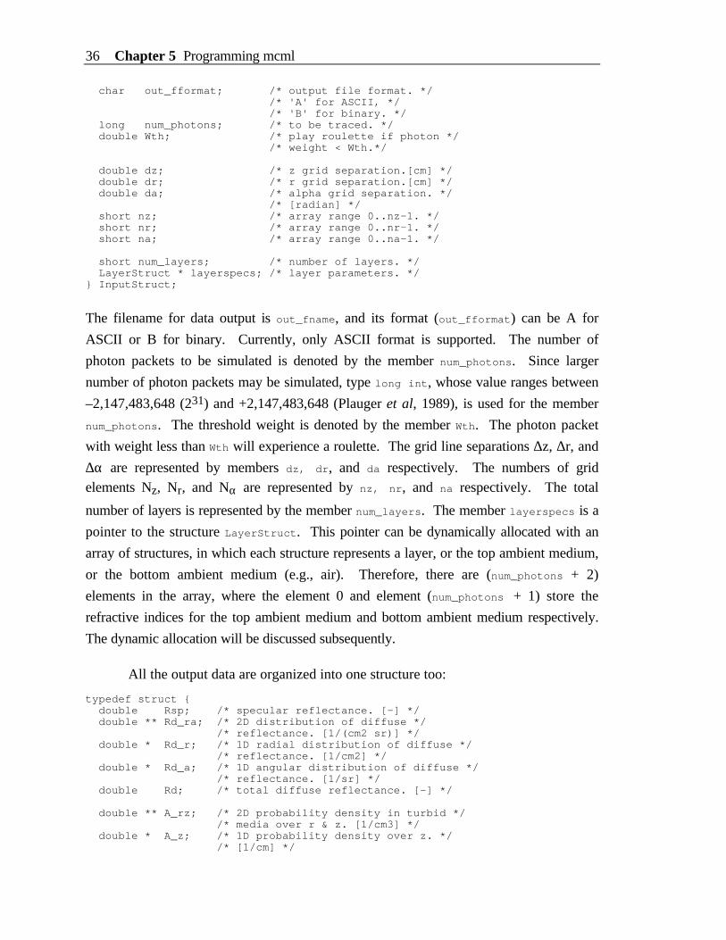
36 Chapter 5 Programming mcml
char out_fformat; /* output file format. */ /* 'A' for ASCII, */ /* 'B' for binary. */ long num_photons; /* to be traced. */ double Wth; /* play roulette if photon */ /* weight < Wth.*/
double dz; /* z grid separation.[cm] */ double dr; /* r grid separation.[cm] */ double da; /* alpha grid separation. */ /* [radian] */ short nz; /* array range 0..nz-1. */ short nr; /* array range 0..nr-1. */ short na; /* array range 0..na-1. */
short num_layers; /* number of layers. */ LayerStruct * layerspecs; /* layer parameters. */ InputStruct;
The filename for data output is out_fname, and its format (out_fformat) can be A for
ASCII or B for binary. Currently, only ASCII format is supported. The number of
photon packets to be simulated is denoted by the member num_photons. Since larger
number of photon packets may be simulated, type long int, whose value ranges between
–2,147,483,648 (231) and +2,147,483,648 (Plauger et al, 1989), is used for the member
num_photons. The threshold weight is denoted by the member Wth. The photon packet
with weight less than Wth will experience a roulette. The grid line separations ∆z, ∆r, and
∆α are represented by members dz, dr, and da respectively. The numbers of gridelements Nz, Nr, and Nα are represented by nz, nr, and na respectively. The total
number of layers is represented by the member num_layers. The member layerspecs is a
pointer to the structure LayerStruct. This pointer can be dynamically allocated with an
array of structures, in which each structure represents a layer, or the top ambient medium,
or the bottom ambient medium (e.g., air). Therefore, there are (num_photons + 2)
elements in the array, where the element 0 and element (num_photons + 1) store the
refractive indices for the top ambient medium and bottom ambient medium respectively.
The dynamic allocation will be discussed subsequently.
All the output data are organized into one structure too:
typedef struct double Rsp; /* specular reflectance. [-] */ double ** Rd_ra; /* 2D distribution of diffuse */ /* reflectance. [1/(cm2 sr)] */ double * Rd_r; /* 1D radial distribution of diffuse */ /* reflectance. [1/cm2] */ double * Rd_a; /* 1D angular distribution of diffuse */ /* reflectance. [1/sr] */ double Rd; /* total diffuse reflectance. [-] */
double ** A_rz; /* 2D probability density in turbid */ /* media over r & z. [1/cm3] */ double * A_z; /* 1D probability density over z. */ /* [1/cm] */
Chapter 5 Programming mcml 37
double * A_l; /* each layer's absorption */ /* probability. [-] */ double A; /* total absorption probability. [-] */
double ** Tt_ra; /* 2D distribution of total */ /* transmittance. [1/(cm2 sr)] */ double * Tt_r; /* 1D radial distribution of */ /* transmittance. [1/cm2] */ double * Tt_a; /* 1D angular distribution of */ /* transmittance. [1/sr] */ double Tt; /* total transmittance. [-] */ OutStruct;
The member Rsp is the specular reflectance. The pointer Rd_ra will be allocated
dynamically, and used equivalently as if it is a 2D array over r and α. Rd_ra is the internalrepresentation of diffuse reflectance Rd(r, α) discussed in Section 4.1. The members Rd_r
and Rd_a are the 1D diffuse reflectance distributions over r and α respectively. Themember Rd is the total diffuse reflectance Rd. The member A_rz is the representation of the
2D internal photon distribution A(r, z) (see Section 4.2). The members A_z and A_l are
the corresponding 1D internal photon distributions with respect to z and layers
respectively. The member A is the probability of photon absorption by the whole tissue.
The members for transmittance are analogous to these for reflectance except that there is
no distinction between unscattered transmittance and diffuse transmittance. All the
transmitted photon weight is scored into the arrays.
In the above defined structures, pointers are used to denote the 2D or 1D arrays.
These pointers are dynamically allocated at run time according to user's specifications.
Therefore, the user can use different numbers of layers or numbers of grid elements
without changing the source code of the program. This provides the flexibility of the
program and the efficiency of memory utilization. The dynamic allocation procedures are
modified from Press (1988). Only 1D array allocation will be presented here, and the
matrix allocation can be found in Appendix B.5 -- "mcmlnr.c".
double *AllocVector(short nl, short nh) double *v; short i;
v=(double *)malloc((unsigned) (nh-nl+1)*sizeof(double)); if (!v) nrerror("allocation failure in vector()");
v -= nl; for(i=nl;i<=nh;i++) v[i] = 0.0; /* init. */ return v;
This function returns a pointer, which points to an array of elements. Each element is a
double precision floating point number. The index range of the array is from nl to nh
38 Chapter 5 Programming mcml
inclusive. In our simulation, nl is always 0, which is the default value in C. This function
also initializes all the elements equal to zero.
5.4 Flowchart of photon tracing
Fig. 5.1 indicates the basic flowchart for the photon tracing part of the Monte
Carlo calculation as described in Chapter 3. Many boxes in the flowchart are direct
implementations of the discussions in Chapter 3. This chart also includes the situation
where the photon packet is in a glass, in which absorption and scattering do not exist. In
this case, the photon packet will be moved to the boundary of the glass layer in the current
photon direction. Then, we have to determine statistically whether the photon packet will
cross the boundary or be reflected according to the Fresnel's formulas.
The box "Launch photon" initializes the photon packet position, direction, weight,
and several other structure members including ds and dsleft in PhotonStruct. The flow
control box "Photon in glass?" determines whether the current layer is a glass layer or
tissue layer.
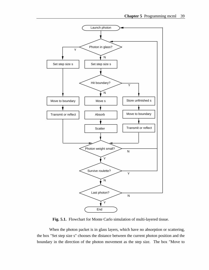
Chapter 5 Programming mcml 39
Fig. 5.1. Flowchart for Monte Carlo simulation of multi-layered tissue.
When the photon packet is in glass layers, which have no absorption or scattering,
the box "Set step size s" chooses the distance between the current photon position and the
boundary in the direction of the photon movement as the step size. The box "Move to
Y
Photon in glass?
Hit boundary?
Move s
Absorb
Scatter
Y
N
N
Launch photon
N
Photon weight small?
Survive roulette?
Last photon?
Y
N
Y
End
N
Y
Set step size sSet step size s
Move to boundary
Transmit or reflect
Store unfinished sMove to boundary
Transmit or reflect
40 Chapter 5 Programming mcml
boundary" updates the position of the photon packet. Now, as the photon packet is on the
boundary, two approaches of processing photon transmission and reflection are supported
in the box "Transmit or reflect" as discussed in Section 3.6. If the constant
PARTIALREFLECTION is zero, the box determines whether the photon packet should cross
the boundary or be reflected according to the Fresnel reflectance in an all-or-none fashion.
If the photon packet is reflected, the propagation direction should be updated. Otherwise,
if the photon packet crosses the interface into another layer of tissue, the propagation
direction and the index to the layer are updated. If the photon packet crosses the
boundary and moves out of the medium, the photon packet is terminated and the photon
weight is scored into the array for reflectance or transmittance depending on where the
photon packet exits. If the constant PARTIALREFLECTION is one, the box "Transmit or
reflect" deals with ambient medium/tissue interface differently. Part of the photon weight
is transmitted to the ambient medium as reflectance or transmittance, and the rest of the
weight will be reflected and continue propagation. Normally we set PARTIALREFLECTION
to 0 because the all-or-none simulation is faster (see Section 3.6).
In tissue layers, the box "Set step size s" sets the step size to the unfinished step
size according to the structure member sleft if sleft is not zero. Otherwise, it sets the
step size according to the interaction coefficient of the medium. With the chosen step size
s, the box "Hit boundary?" identifies whether the step size is long enough to hit the
boundary of the current layer.
If the step does not hit the boundary, then the box "Move s" will update the
position of the photon packet. Then, the box "Absorb" will deposit a portion of the
photon packet weight in the local grid element, and the box "Scatter" will determine the
new traveling direction for the rest of the photon packet after absorption.
If the step hits the boundary, then the step size s is foreshortened. The
foreshortened step size is the distance between the photon position and the boundary in
the direction of the photon movement, and the unfinished step size is stored by the box
"Store unfinished s". The stored unfinished step size in dimensionless units will be used by
the box "Set step size s" for tissue layers to generate the next step size. The next two
boxes "Move to boundary" and "Transmit or reflect" function the same as for the glass
layer.
At this point, the photon weight and the structure member dead are checked in the
box "Photon weight small?". If the photon packet is dead, it will jump to the box "Last
Chapter 5 Programming mcml 41
photon?" (transition not shown in the flowchart). If the photon packet is still alive and its
weight exceeds Wth, it will start the next step of propagation. If the photon packet is still
alive and its weight is lower than Wth, it has to experience a roulette in the box "Survive
roulette?". If the photon packet survives the roulette, it will start the next step of
propagation. Otherwise, the photon packet is terminated and the box "Last photon?"
determines whether to end the simulation or to start tracing a new photon packet.
5.5 Flow of the program mcml
A flow graph of the mcml source code has been generated using the UNIX
command cflow under SunOS. Each line of output begins with a reference number, i.e., a
line number, followed by a suitable number of tabs indicating the level, then the name of
the global (normally only a function not defined as an external or beginning with an
underscore), a colon, and its definition. The definition consists of an abstract type
declaration (for example, char *), and delimited by angle brackets, the name of the source
file and the line number where the definition was found.
Once a definition of a name has been printed, subsequent references to that
name contain only the reference number of the line where the definition may be found.
For undefined references, only <> is printed.
The list in Fig. 5.2 is generated by command: cflow -d2 mcml*.c. The option "-
d2" limits the nesting depth to 2. The command output with all the nesting levels is shown
in Appendix A.
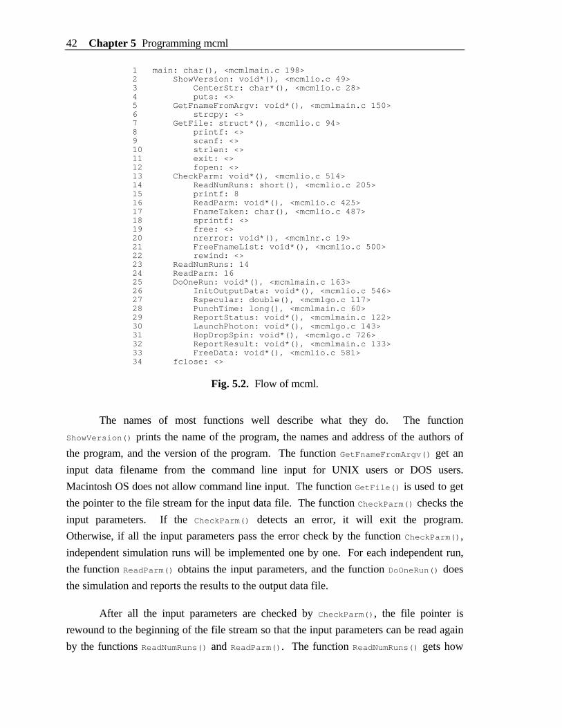
42 Chapter 5 Programming mcml
1 main: char(), <mcmlmain.c 198>2 ShowVersion: void*(), <mcmlio.c 49>3 CenterStr: char*(), <mcmlio.c 28>4 puts: <>5 GetFnameFromArgv: void*(), <mcmlmain.c 150>6 strcpy: <>7 GetFile: struct*(), <mcmlio.c 94>8 printf: <>9 scanf: <>10 strlen: <>11 exit: <>12 fopen: <>13 CheckParm: void*(), <mcmlio.c 514>14 ReadNumRuns: short(), <mcmlio.c 205>15 printf: 816 ReadParm: void*(), <mcmlio.c 425>17 FnameTaken: char(), <mcmlio.c 487>18 sprintf: <>19 free: <>20 nrerror: void*(), <mcmlnr.c 19>21 FreeFnameList: void*(), <mcmlio.c 500>22 rewind: <>23 ReadNumRuns: 1424 ReadParm: 1625 DoOneRun: void*(), <mcmlmain.c 163>26 InitOutputData: void*(), <mcmlio.c 546>27 Rspecular: double(), <mcmlgo.c 117>28 PunchTime: long(), <mcmlmain.c 60>29 ReportStatus: void*(), <mcmlmain.c 122>30 LaunchPhoton: void*(), <mcmlgo.c 143>31 HopDropSpin: void*(), <mcmlgo.c 726>32 ReportResult: void*(), <mcmlmain.c 133>33 FreeData: void*(), <mcmlio.c 581>34 fclose: <>
Fig. 5.2. Flow of mcml.
The names of most functions well describe what they do. The function
ShowVersion() prints the name of the program, the names and address of the authors of
the program, and the version of the program. The function GetFnameFromArgv() get an
input data filename from the command line input for UNIX users or DOS users.
Macintosh OS does not allow command line input. The function GetFile() is used to get
the pointer to the file stream for the input data file. The function CheckParm() checks the
input parameters. If the CheckParm() detects an error, it will exit the program.
Otherwise, if all the input parameters pass the error check by the function CheckParm(),
independent simulation runs will be implemented one by one. For each independent run,
the function ReadParm() obtains the input parameters, and the function DoOneRun() does
the simulation and reports the results to the output data file.
After all the input parameters are checked by CheckParm(), the file pointer is
rewound to the beginning of the file stream so that the input parameters can be read again
by the functions ReadNumRuns() and ReadParm(). The function ReadNumRuns() gets how
Chapter 5 Programming mcml 43
many independent simulations are to be specified in this input data file. The function
ReadParm() only reads the input parameters for one independent run.
Under the function DoOneRun(), the function PunchTime() provides the user time
and the real time used so far by the current simulation run. The function ReportStatus()
fetches the real time and predicts when the current simulation run will finish. However,
these timing functions will not work if the source code is compiled by a GNU C compiler.
The function LaunchPhoton() initializes a photon packet. The function HopDropSpin()
moves the photon packet, deposits some photon packet weight, scatters the packet, and
deals with the boundary. After the given number of photon packets are traced, the results
are properly processed (see Chapter 4) and then written to an output file by the function
ReportResult().
5.6 Multiple simulations
The program can do any number of independent simulations sequentially without
being subject to memory limit. It checks the parameters of one simulation after another
before starting the simulation. If it detects an error in the input data file, the program
stops the execution. Otherwise, it reads in the parameters of one independent simulation
at a time and starts the simulation. At the end of the simulation, it writes the results to the
output data file whose name is specified by the input data file. The next independent run
will be processed thereafter. The users should try to make sure not to use the same output
filenames for different simulations, although the program checks against duplicated output
filenames.
To check against duplicated filenames specified in an input data file, we set up a
linear linked list to store the filenames specified in the input data file. Each new filename
is compared with every node of the filename list. If the name is already taken, the
program notifies the user of the name, and exits to the system. Otherwise, if no filename
is duplicated, the program deletes the filename list to release the memory, and continues
execution.
5.7 Timing profile of the program
The timing profile of the program mcml indicates how to improve the efficiency of
the program by logging how much time the program spends on each function. Profilers
are available in a few compilers including C compilers of UNIX operating systems, and
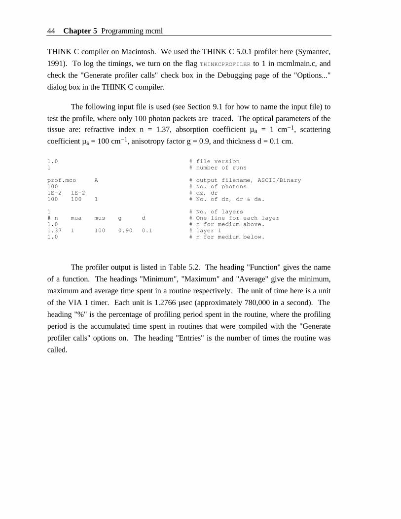
44 Chapter 5 Programming mcml
THINK C compiler on Macintosh. We used the THINK C 5.0.1 profiler here (Symantec,
1991). To log the timings, we turn on the flag THINKCPROFILER to 1 in mcmlmain.c, and
check the "Generate profiler calls" check box in the Debugging page of the "Options..."
dialog box in the THINK C compiler.
The following input file is used (see Section 9.1 for how to name the input file) to
test the profile, where only 100 photon packets are traced. The optical parameters of thetissue are: refractive index n = 1.37, absorption coefficient µa = 1 cm−1, scattering
coefficient µs = 100 cm−1, anisotropy factor g = 0.9, and thickness d = 0.1 cm.
1.0 # file version1 # number of runs
prof.mco A # output filename, ASCII/Binary100 # No. of photons1E-2 1E-2 # dz, dr100 100 1 # No. of dz, dr & da.
1 # No. of layers# n mua mus g d # One line for each layer1.0 # n for medium above.1.37 1 100 0.90 0.1 # layer 11.0 # n for medium below.
The profiler output is listed in Table 5.2. The heading "Function" gives the name
of a function. The headings "Minimum", "Maximum" and "Average" give the minimum,
maximum and average time spent in a routine respectively. The unit of time here is a unit
of the VIA 1 timer. Each unit is 1.2766 µsec (approximately 780,000 in a second). The
heading "%" is the percentage of profiling period spent in the routine, where the profiling
period is the accumulated time spent in routines that were compiled with the "Generate
profiler calls" options on. The heading "Entries" is the number of times the routine was
called.
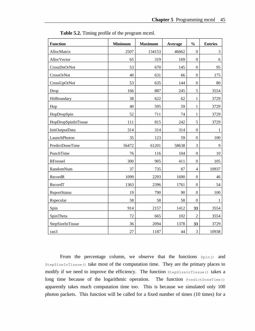
Chapter 5 Programming mcml 45
Table 5.2. Timing profile of the program mcml.
Function Minimum Maximum Average % Entries
AllocMatrix 2507 134153 46662 0 3
AllocVector 65 319 169 0 6
CrossDnOrNot 53 670 145 0 95
CrossOrNot 40 631 66 0 175
CrossUpOrNot 53 635 144 0 80
Drop 166 887 245 5 3554
HitBoundary 38 622 62 1 3729
Hop 40 595 59 1 3729
HopDropSpin 52 711 74 1 3729
HopDropSpinInTissue 111 815 242 5 3729
InitOutputData 314 314 314 0 1
LaunchPhoton 35 123 59 0 100
PredictDoneTime 56472 61201 58638 3 9
PunchTime 76 116 104 0 10
RFresnel 300 905 411 0 105
RandomNum 37 735 67 4 10937
RecordR 1099 2293 1690 0 46
RecordT 1363 2396 1761 0 54
ReportStatus 19 790 90 0 100
Rspecular 58 58 58 0 1
Spin 914 2157 1412 33 3554
SpinTheta 72 665 102 2 3554
StepSizeInTissue 36 2094 1378 33 3729
ran3 27 1187 44 3 10938
From the percentage column, we observe that the functions Spin() and
StepSizeInTissue() take most of the computation time. They are the primary places to
modify if we need to improve the efficiency. The function StepSizeinTissue() takes a
long time because of the logarithmic operation. The function PredictDoneTime()
apparently takes much computation time too. This is because we simulated only 100
photon packets. This function will be called for a fixed number of times (10 times) for a

46 Chapter 5 Programming mcml
simulation no matter how many photon packets are simulated. Therefore, its percentage
will decrease linearly with the number of photon packets to be simulated. Note that we
made the profiler include only the main part of the simulation (See file mcmlmain.c in
Appendix B). Therefore, the functions for input or output of data are not included since
they do not scale up as the number of photon packets to be simulated increases.

Chapter 6 Computation Results of mcml and Verification 47
6. Computation Results of mcml and Verification
Some computation results are described in this chapter as examples, and some of
them are compared with the results from other theory or with the Monte Carlo simulation
results from other investigators to verify the program.
6.1 Total diffuse reflectance and total transmittance
We computed the total diffuse reflectance and total transmittance of a slab of
turbid medium with the following optical properties: relative refractive index n = 1,absorption coefficient µa = 10 cm−1, scattering coefficient µs = 90 cm−1, anisotropy factor
g = 0.75, and thickness d = 0.02 cm. Ten Monte Carlo simulations of 50,000 photon
packets each are completed. Then, the averages and the standard errors of the total
diffuse reflectance and total transmittance are computed (Table 6.1). The table also lists
the results from van de Hulst's table (van de Hulst, 1980) and from Monte Carlo
simulations by Prahl et al. (1989). All results agree with each other.
Table 6.1. Verification of the total diffuse reflectance and the total
transmittance in a slab with a matched boundary.
The columns "Rd Average" and "Rd Error" are the average and the standard error of the
total diffuse reflectance respectively, while the columns "Tt Average" and "Tt Error" are
the average and the standard error of the total transmittance.
For a semi-infinite turbid medium that has mismatched refractive index with the
ambient medium, the average and the standard error of the total diffuse reflectance are
computed similarly, and compared in Table 6.2 with Giovanelli's (1955) results and Monte
Carlo simulation results by Prahl et al. (1989). The medium has the following opticalproperties: relative refractive index n = 1.5, µa = 10 cm−1, µs = 90 cm−1, g = 0 (isotropic
scattering). Ten Monte Carlo simulations of 5,000 photon packets each are completed to
compute the average and the standard error of the total diffuse reflectance.
Source Rd Average Rd Error Tt Average Tt Error
van de Hulst, 1980 0.09739 0.66096
mcml 0.09734 0.00035 0.66096 0.00020
Prahl et al., 1989 0.09711 0.00033 0.66159 0.00049
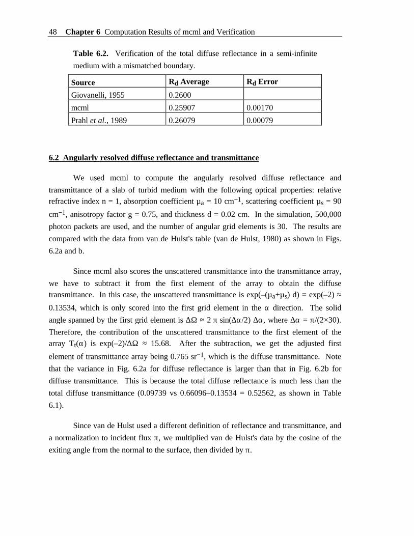
48 Chapter 6 Computation Results of mcml and Verification
Table 6.2. Verification of the total diffuse reflectance in a semi-infinite
medium with a mismatched boundary.
Source Rd Average Rd Error
Giovanelli, 1955 0.2600
mcml 0.25907 0.00170
Prahl et al., 1989 0.26079 0.00079
6.2 Angularly resolved diffuse reflectance and transmittance
We used mcml to compute the angularly resolved diffuse reflectance and
transmittance of a slab of turbid medium with the following optical properties: relativerefractive index n = 1, absorption coefficient µa = 10 cm−1, scattering coefficient µs = 90
cm−1, anisotropy factor g = 0.75, and thickness d = 0.02 cm. In the simulation, 500,000
photon packets are used, and the number of angular grid elements is 30. The results are
compared with the data from van de Hulst's table (van de Hulst, 1980) as shown in Figs.
6.2a and b.
Since mcml also scores the unscattered transmittance into the transmittance array,
we have to subtract it from the first element of the array to obtain the diffusetransmittance. In this case, the unscattered transmittance is exp(–(µa+µs) d) = exp(–2) ≈
0.13534, which is only scored into the first grid element in the α direction. The solid
angle spanned by the first grid element is ∆Ω ≈ 2 π sin(∆α/2) ∆α, where ∆α = π/(2×30).
Therefore, the contribution of the unscattered transmittance to the first element of thearray Tt(α) is exp(–2)/∆Ω ≈ 15.68. After the subtraction, we get the adjusted first
element of transmittance array being 0.765 sr−1, which is the diffuse transmittance. Note
that the variance in Fig. 6.2a for diffuse reflectance is larger than that in Fig. 6.2b for
diffuse transmittance. This is because the total diffuse reflectance is much less than the
total diffuse transmittance (0.09739 vs 0.66096–0.13534 = 0.52562, as shown in Table
6.1).
Since van de Hulst used a different definition of reflectance and transmittance, and
a normalization to incident flux π, we multiplied van de Hulst's data by the cosine of the
exiting angle from the normal to the surface, then divided by π.
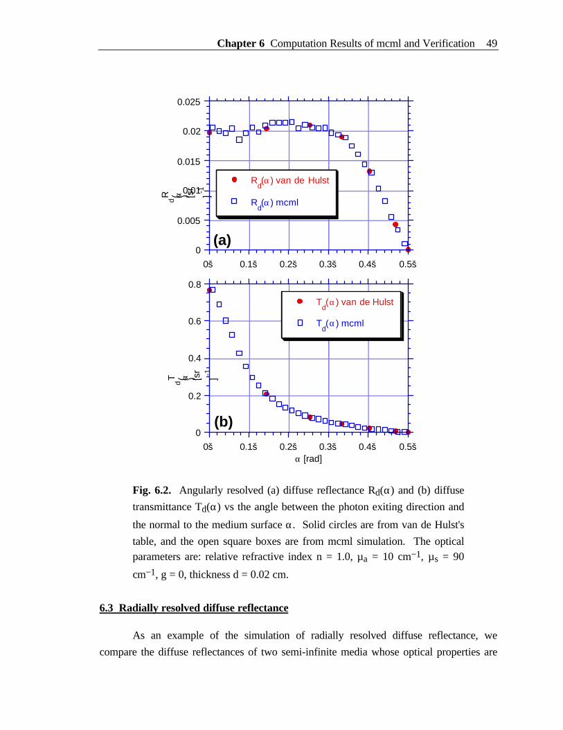
Chapter 6 Computation Results of mcml and Verification 49
0
0.005
0.01
0.015
0.02
0.025
Rd( α ) [s
r -1 ]
0š 0.1š 0.2š 0.3š 0.4š 0.5š
Rd(α) van de Hulst
Rd(α) mcml
(a)
0
0.2
0.4
0.6
0.8
0š
Td( α ) [s
r -1 ]
0.1š 0.2š 0.3š 0.4š 0.5š
(b)
Td(α) van de Hulst
Td(α) mcml
α [rad]
Fig. 6.2. Angularly resolved (a) diffuse reflectance Rd(α) and (b) diffuse
transmittance Td(α) vs the angle between the photon exiting direction and
the normal to the medium surface α. Solid circles are from van de Hulst's
table, and the open square boxes are from mcml simulation. The opticalparameters are: relative refractive index n = 1.0, µa = 10 cm−1, µs = 90
cm−1, g = 0, thickness d = 0.02 cm.
6.3 Radially resolved diffuse reflectance
As an example of the simulation of radially resolved diffuse reflectance, we
compare the diffuse reflectances of two semi-infinite media whose optical properties are
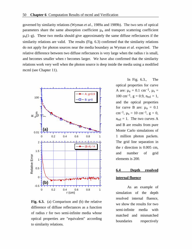
50 Chapter 6 Computation Results of mcml and Verification
governed by similarity relations (Wyman et al., 1989a and 1989b). The two sets of opticalparameters share the same absorption coefficient µa and transport scattering coefficient
µs(1–g). These two media should give approximately the same diffuse reflectances if the
similarity relations are valid. The results (Fig. 6.3) confirmed that the similarity relations
do not apply for photon sources near the media boundary as Wyman et al. expected. The
relative difference between two diffuse reflectances is very large when the radius r is small,
and becomes smaller when r becomes larger. We have also confirmed that the similarity
relations work very well when the photon source is deep inside the media using a modified
mcml (see Chapter 11).
In Fig. 6.3., The
optical properties for curveA are: µa = 0.1 cm−1, µs =
100 cm−1, g = 0.9, nrel = 1,
and the optical propertiesfor curve B are: µa = 0.1
cm−1, µs = 10 cm−1, g = 0,
nrel = 1. The two curves A
and B are results from pure
Monte Carlo simulations of
1 million photon packets.
The grid line separation in
the r direction is 0.005 cm,
and number of grid
elements is 200.
6.4 Depth resolved
internal fluence
As an example of
simulation of the depth
resolved internal fluence,
we show the results for two
semi-infinite media with
matched and mismatched
boundaries respectively
0.01
1
100
0 0.2
R d (cm
-2 )
0.4 0.6 0.8 1
A: g=0.9
B: g=0
(a)
-0.5
0
0.5
1
1.5
2
Rel
ativ
e E
rror
0 0.2 0.4 0.6 0.8 1r (cm)
(b)
(B-A) / A
Fig. 6.3. (a) Comparison and (b) the relative
difference of diffuse reflectances as a function
of radius r for two semi-infinite media whose
optical properties are "equivalent" according
to similarity relations.
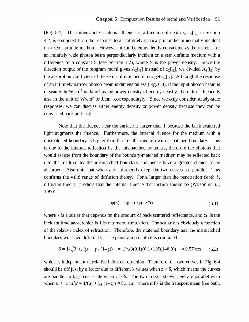
Chapter 6 Computation Results of mcml and Verification 51
(Fig. 6.4). The dimensionless internal fluence as a function of depth z, φz[iz] in Section
4.2, is computed from the response to an infinitely narrow photon beam normally incident
on a semi-infinite medium. However, it can be equivalently considered as the response of
an infinitely wide photon beam perpendicularly incident on a semi-infinite medium with a
difference of a constant S (see Section 4.2), where S is the power density. Since thedirection output of the program mcml gives Az[iz] instead of φz[iz], we divided Az[iz] by
the absorption coefficient of the semi-infinite medium to get φz[iz]. Although the response
of an infinitely narrow photon beam is dimensionless (Fig. 6.4), if the input photon beam is
measured in W/cm2 or J/cm2 as the power density of energy density, the unit of fluence is
also in the unit of W/cm2 or J/cm2 correspondingly. Since we only consider steady-state
responses, we can discuss either energy density or power density because they can be
converted back and forth.
Note that the fluence near the surface is larger than 1 because the back scattered
light augments the fluence. Furthermore, the internal fluence for the medium with a
mismatched boundary is higher than that for the medium with a matched boundary. This
is due to the internal reflection by the mismatched boundary, therefore the photons that
would escape from the boundary of the boundary-matched medium may be reflected back
into the medium by the mismatched boundary and hence have a greater chance to be
absorbed. Also note that when z is sufficiently deep, the two curves are parallel. This
confirms the valid range of diffusion theory. For z larger than the penetration depth δ,
diffusion theory predicts that the internal fluence distribution should be (Wilson et al.,
1990):
φ(z) = φ0 k exp(–z/δ) (6.1)
where k is a scalar that depends on the amount of back scattered reflectance, and φ0 is the
incident irradiance, which is 1 in our mcml simulation. The scalar k is obviously a function
of the relative index of refraction. Therefore, the matched boundary and the mismatched
boundary will have different k. The penetration depth δ is computed:
δ = 1/ 3 µa (µs + µs (1–g)) = 1/ 3(0.1)(0.1+100(1–0.9)) ≈ 0.57 cm (6.2)
which is independent of relative index of refraction. Therefore, the two curves in Fig. 6.4
should be off just by a factor due to different k values when z > δ, which means the curves
are parallel in log-linear scale when z > δ. The two curves shown here are parallel evenwhen z > 1 mfp' = 1/(µs + µs (1–g)) ≈ 0.1 cm, where mfp' is the transport mean free path.
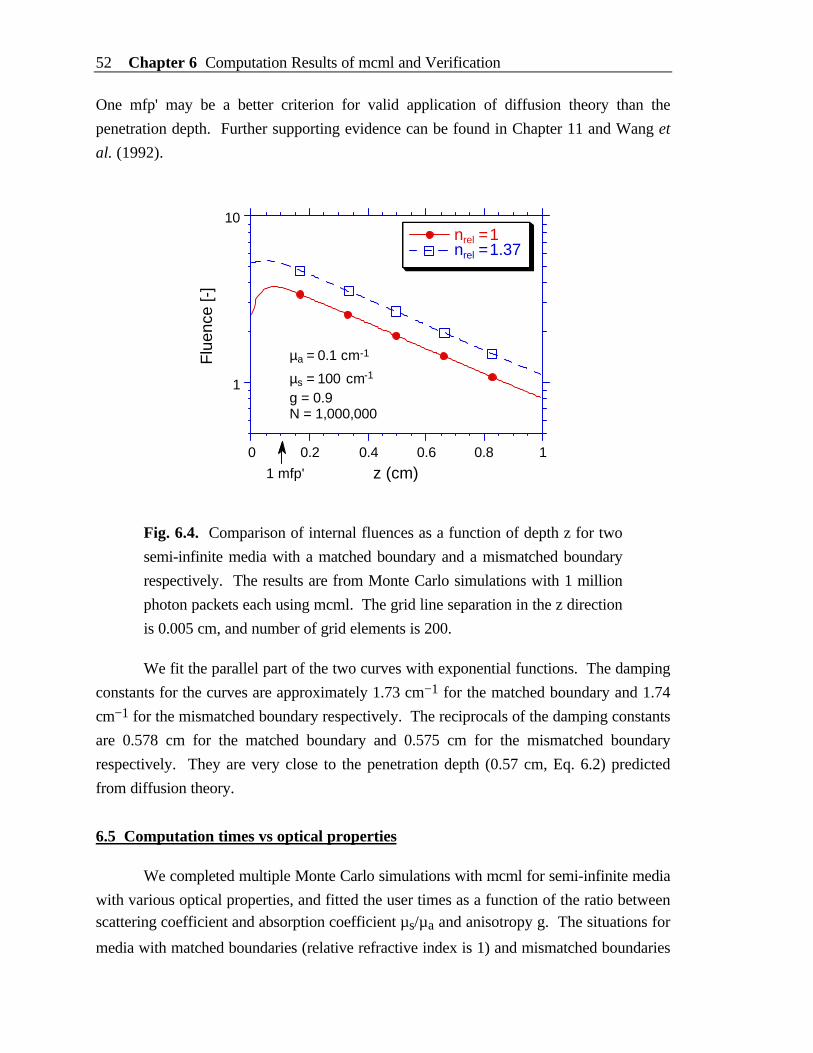
52 Chapter 6 Computation Results of mcml and Verification
One mfp' may be a better criterion for valid application of diffusion theory than the
penetration depth. Further supporting evidence can be found in Chapter 11 and Wang et
al. (1992).
1
10
0 0.2
Flu
ence
[-]
0.4 0.6 0.8 1
nrel = 1nrel = 1.37
z (cm)
µa = 0.1 cm-1
µs = 100 cm-1
g = 0.9N = 1,000,000
1 mfp'
Fig. 6.4. Comparison of internal fluences as a function of depth z for two
semi-infinite media with a matched boundary and a mismatched boundary
respectively. The results are from Monte Carlo simulations with 1 million
photon packets each using mcml. The grid line separation in the z direction
is 0.005 cm, and number of grid elements is 200.
We fit the parallel part of the two curves with exponential functions. The damping
constants for the curves are approximately 1.73 cm−1 for the matched boundary and 1.74
cm−1 for the mismatched boundary respectively. The reciprocals of the damping constants
are 0.578 cm for the matched boundary and 0.575 cm for the mismatched boundary
respectively. They are very close to the penetration depth (0.57 cm, Eq. 6.2) predicted
from diffusion theory.
6.5 Computation times vs optical properties
We completed multiple Monte Carlo simulations with mcml for semi-infinite media
with various optical properties, and fitted the user times as a function of the ratio betweenscattering coefficient and absorption coefficient µs/µa and anisotropy g. The situations for
media with matched boundaries (relative refractive index is 1) and mismatched boundaries
Chapter 6 Computation Results of mcml and Verification 53
(relative refractive index is not 1) will be presented separately. Note that the user time is
whatever the system allocates to the running of the program, as opposed to the real time
which is wall-clock time. In a time-shared system, they need not be the same, and the real
time of the same run may not be reproduced depending on the status of the system. In
mcml, the user time is reported to the output data file, and the real time is used to predict
when the simulation finishes during the simulation.
Before starting multiple mcml simulations for various optical properties, we know
that the time required to finish tracing a photon packet is proportional to the number of
steps that a photon packet takes until being terminated. According to the rules for photon
propagation described in Chapter 3, this number of steps should not be dependent on theabsolute values of scattering coefficient µs and absorption coefficient µa, but their ratio.
Therefore, we keep one of the two parameters constant (e.g., µs = 100 cm−1), and vary
the other one (e.g., µa).
Matched boundary
For media with matched boundaries (relative refractive index nrel is 1), we finished
multiple mcml simulations of 10,000 photon packets each for various absorptioncoefficients µa and anisotropy factors while keeping the scattering coefficient µs fixed to
100 cm−1. The results are listed in Table 6.3, where the ratios between the scattering
coefficient and the absorption coefficient are tabulated, instead of the two coefficients
themselves separately, and the user

54 Chapter 6 Computation Results of mcml and Verification
Table. 6.3. Computation times for various media with matched
boundaries. The column "Predicted User Time" is the computed values
using Eqs. 6.1-6.3 presented later. The column "Error" is equal to
(Predicted User Time – User Time)/(User Time)*100.
µs/µa g User Time(sec./1000 photons)
Predicted User Time(sec./1000 photons)
Error(%)
0.2 0 0.43 0.36 –16.151 0 0.78 0.81 3.582 0 1.10 1.15 4.4210 0 2.59 2.56 –0.9920 0 3.66 3.62 –0.97100 0 8.46 8.10 –4.23200 0 12.27 11.46 –6.641000 0 29.61 25.61 –13.49
0.2 0.1 0.40 0.38 –5.041 0.1 0.80 0.86 7.192 0.1 1.10 1.22 10.7010 0.1 2.80 2.75 –1.8220 0.1 3.90 3.90 0.10100 0.1 9.80 8.81 –10.07200 0.1 13.20 12.52 –5.191000 0.1 28.60 28.25 –1.21
0.2 0.5 0.50 0.45 –9.541 0.5 1.00 1.08 7.712 0.5 1.40 1.57 11.8010 0.5 3.50 3.73 6.4920 0.5 5.30 5.42 2.19100 0.5 12.10 12.90 6.60200 0.5 17.90 18.74 4.711000 0.5 40.60 44.63 9.93
0.2 0.9 0.50 0.49 –1.831 0.9 1.20 1.35 12.742 0.9 1.90 2.09 10.2010 0.9 6.30 5.77 –8.3920 0.9 9.80 8.93 –8.86100 0.9 25.80 24.62 –4.58200 0.9 38.10 38.10 0.001000 0.9 95.30 105.02 10.20
0.2 0.99 0.50 0.42 –16.181 0.99 1.20 1.42 18.682 0.99 2.10 2.41 14.8510 0.99 8.80 8.20 –6.8720 0.99 16.50 13.88 –15.89100 0.99 60.60 47.16 –22.18200 0.99 97.20 79.86 –17.841000 0.99 248.80 271.37 9.07
Chapter 6 Computation Results of mcml and Verification 55
times are converted to seconds per 1000, instead of 10,000, photon packets. The columns
"Predicted User Time" and "Error" will be discussed subsequently
We plotted the user times as a function of the ratio between the scattering
coefficient and the absorption coefficient for each anisotropy factor g in a log-log scale
(Fig. 6.5). For each anisotropy factor g, the higher the ratio between the scattering
coefficient and the absorption coefficient, the longer the user time. This is because thephoton packets in media of higher ratio µs/µa, compared with media of lower ratio, can
jump more steps before reaching the threshold weight and hence having a chance to be
terminated. Therefore, the Monte Carlo simulation of low absorbing medium is very slow.
If the diffuse reflectance as a function of r in a low absorption semi-infinite turbid medium
is the only physical quantity to be computed, a hybrid model of pure Monte Carlo
simulation and diffusion theory (Wang et al., 1992) is a much faster model than pure
Monte Carlo simulations. The speed of the hybrid model is not so sensitive to the ratio
between the scattering coefficient and the absorption coefficient.
For the same ratio between the scattering coefficient and the absorption
coefficient, the larger the anisotropy factor g, the longer the user time. This is because
that the photon packets in media of larger anisotropy factors g have less chance to be
reflected out of the media because the scatterings are more forward directed, and hence to
be terminated.
For each anisotropy factor g, the data points are well aligned in the log-log plot.
This means that we can fit the data points for each anisotropy factor g with a power
function. The fitted lines are presented in Fig. 6.5.
The two fitting coefficients C1(g) and C2(g) are dependent on the anisotropy
factor g. The fitting coefficients C1(g) are plotted against the anisotropy factor g in a log-
linear scale (Fig. 6.6a), and can be fitted with an exponential function. Similarly, thefitting coefficients C2(g) are plotted against (1 – g) in a linear-log scale (Fig. 6.6b), and
can be fitted with a logarithmic function. These three fittings are summarized as the
following empirical formulas:
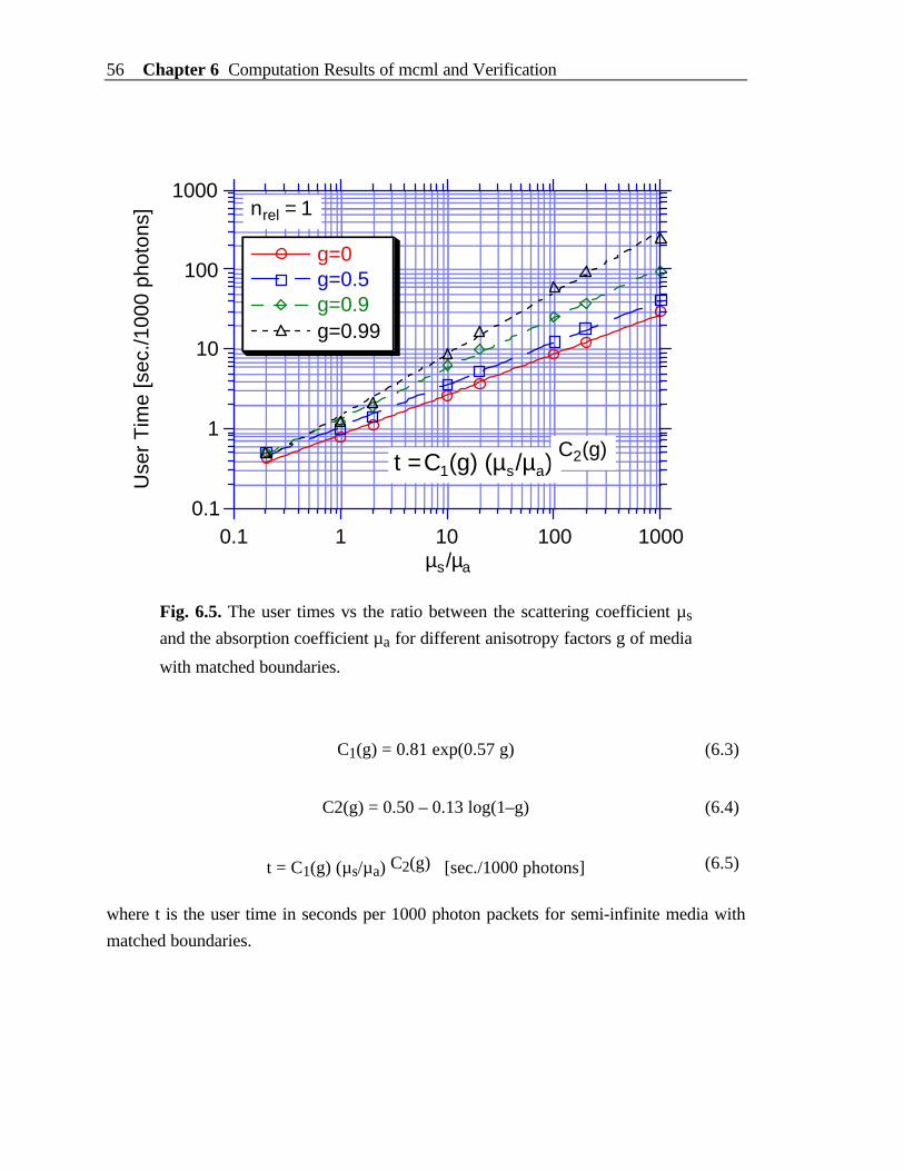
56 Chapter 6 Computation Results of mcml and Verification
0.1
1
10
100
Use
r T
ime
[sec
./100
0 ph
oton
s]
1000
0.1 1 10 100µs/µa
1000
g=0g=0.5g=0.9g=0.99
t = C1(g) (µs/µa)C2(g)
nrel = 1
Fig. 6.5. The user times vs the ratio between the scattering coefficient µs
and the absorption coefficient µa for different anisotropy factors g of media
with matched boundaries.
C1(g) = 0.81 exp(0.57 g) (6.3)
C2(g) = 0.50 – 0.13 log(1–g) (6.4)
t = C1(g) (µs/µa) C2(g) [sec./1000 photons] (6.5)
where t is the user time in seconds per 1000 photon packets for semi-infinite media with
matched boundaries.
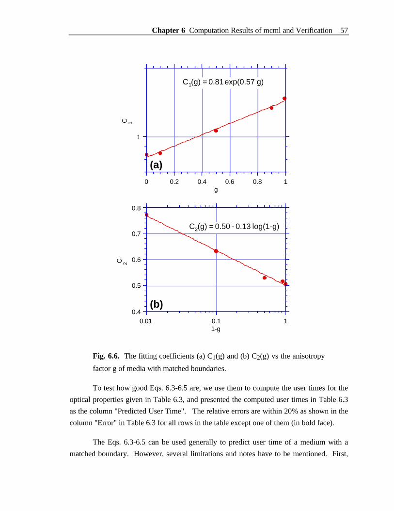
Chapter 6 Computation Results of mcml and Verification 57
1
0
C 1
0.2 0.4 0.6 0.8 1
C1(g) = 0.81 exp(0.57 g)
g
(a)
0.4
0.5
0.6C 2
0.7
0.8
0.01 0.1
C2(g) = 0.50 - 0.13 log(1-g)
1-g1
(b)
Fig. 6.6. The fitting coefficients (a) C1(g) and (b) C2(g) vs the anisotropy
factor g of media with matched boundaries.
To test how good Eqs. 6.3-6.5 are, we use them to compute the user times for the
optical properties given in Table 6.3, and presented the computed user times in Table 6.3
as the column "Predicted User Time". The relative errors are within 20% as shown in the
column "Error" in Table 6.3 for all rows in the table except one of them (in bold face).
The Eqs. 6.3-6.5 can be used generally to predict user time of a medium with a
matched boundary. However, several limitations and notes have to be mentioned. First,
58 Chapter 6 Computation Results of mcml and Verification
the anisotropy factor g is limited to less than 0.99, and the accuracy is unknown for g >0.99 because the fitting coefficient C2(g) approaches infinity when g approaches 1.
Second, these equations are based on mcml simulations on a Sun SPARCstation 2.
Therefore, we expect a scale factor for Eq. 6.5 or the values in Table 6.3 on a different
computer system. This scale factor can be determined by simulating one or several media
with optical properties in Table 6.3 using mcml running on your computer system and
taking the ratio between the user time on your machine and the user time in Table 6.3.
Third, the speed of mcml is related to the threshold weight in the program mcml (WEIGHT
in Table 5.1), which is normally 1×10 –4 (See Table 5.1), and the chance of surviving a
roulette (CHANCE in Table 5.1), which is normally 0.1 (See Table 5.1). If these two
parameters are changed, Eqs. 6.3-6.5 are no longer valid. It is unexplored yet how these
two parameters will affect the user times.
Mismatched boundary
We repeat the above process to media with mismatched boundaries (relativerefractive index nrel 1). We finished multiple mcml simulations of 1,000 (instead of
10,000 for matched boundaries) photon packets each for various absorption coefficients
and anisotropy factors while keeping the scattering coefficient fixed to 100 cm−1 and the
relative refractive index to 1.37, which is typical for human tissues in visible or infrared
wavelength. The results are listed in Table 6.4.
We plotted the user times as a function of the ratio between the scattering
coefficient and the absorption coefficient for each anisotropy factor g in a log-log scale(Fig. 6.7). Then, the fitting coefficients C1(g) and C2(g) are plotted with respect to g and
(1–g) respectively (Fig. 6.8a and b), and fitted with an exponential function and a
logarithmic function correspondingly. The fittings give the following empirical formulas:
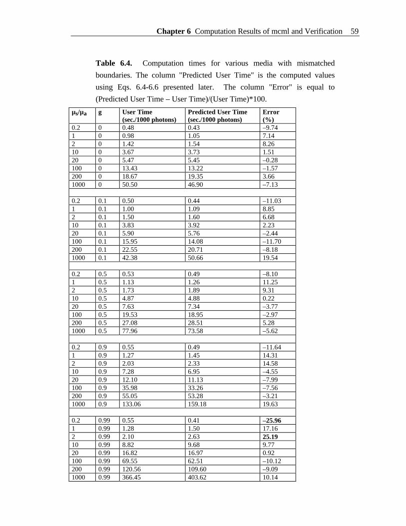
Chapter 6 Computation Results of mcml and Verification 59
Table 6.4. Computation times for various media with mismatched
boundaries. The column "Predicted User Time" is the computed values
using Eqs. 6.4-6.6 presented later. The column "Error" is equal to
(Predicted User Time – User Time)/(User Time)*100.
µs/µa g User Time(sec./1000 photons)
Predicted User Time(sec./1000 photons)
Error(%)
0.2 0 0.48 0.43 –9.741 0 0.98 1.05 7.142 0 1.42 1.54 8.2610 0 3.67 3.73 1.5120 0 5.47 5.45 –0.28100 0 13.43 13.22 –1.57200 0 18.67 19.35 3.661000 0 50.50 46.90 –7.13
0.2 0.1 0.50 0.44 –11.031 0.1 1.00 1.09 8.852 0.1 1.50 1.60 6.6810 0.1 3.83 3.92 2.2320 0.1 5.90 5.76 –2.44100 0.1 15.95 14.08 –11.70200 0.1 22.55 20.71 –8.181000 0.1 42.38 50.66 19.54
0.2 0.5 0.53 0.49 –8.101 0.5 1.13 1.26 11.252 0.5 1.73 1.89 9.3110 0.5 4.87 4.88 0.2220 0.5 7.63 7.34 –3.77100 0.5 19.53 18.95 –2.97200 0.5 27.08 28.51 5.281000 0.5 77.96 73.58 –5.62
0.2 0.9 0.55 0.49 –11.641 0.9 1.27 1.45 14.312 0.9 2.03 2.33 14.5810 0.9 7.28 6.95 –4.5520 0.9 12.10 11.13 –7.99100 0.9 35.98 33.26 –7.56200 0.9 55.05 53.28 –3.211000 0.9 133.06 159.18 19.63
0.2 0.99 0.55 0.41 –25.961 0.99 1.28 1.50 17.162 0.99 2.10 2.63 25.1910 0.99 8.82 9.68 9.7720 0.99 16.82 16.97 0.92100 0.99 69.55 62.51 –10.12200 0.99 120.56 109.60 –9.091000 0.99 366.45 403.62 10.14
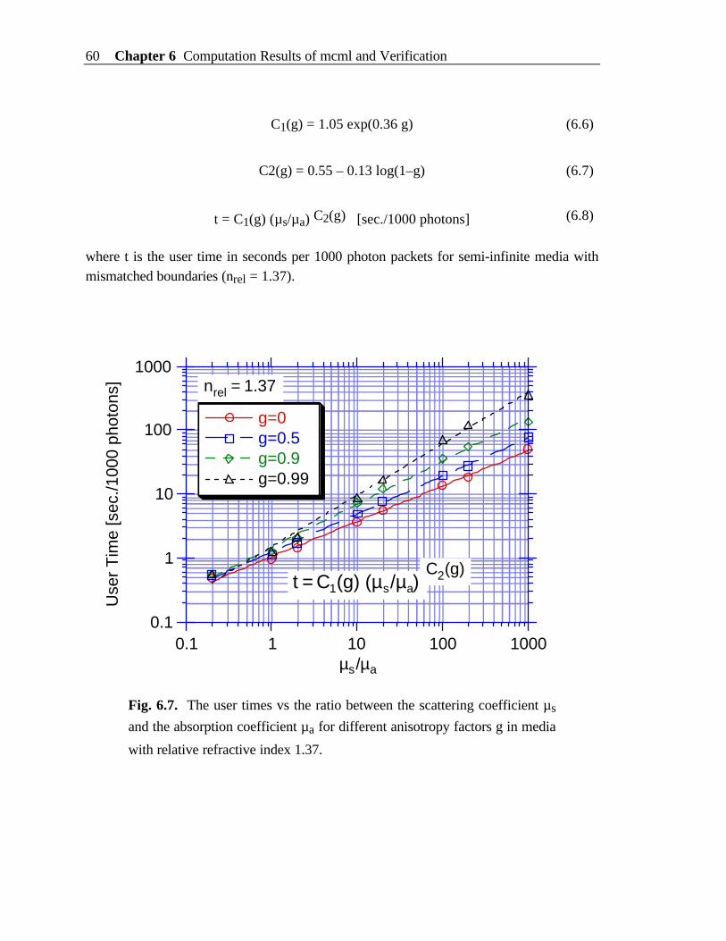
60 Chapter 6 Computation Results of mcml and Verification
C1(g) = 1.05 exp(0.36 g) (6.6)
C2(g) = 0.55 – 0.13 log(1–g) (6.7)
t = C1(g) (µs/µa) C2(g) [sec./1000 photons] (6.8)
where t is the user time in seconds per 1000 photon packets for semi-infinite media withmismatched boundaries (nrel = 1.37).
0.1
1
10
100
1000
0.1 1
Use
r T
ime
[sec
./100
0 ph
oton
s]
10 100 1000
g=0g=0.5g=0.9g=0.99
µs/µa
C2(g)
nrel = 1.37
t = C1(g) (µs/µa)
Fig. 6.7. The user times vs the ratio between the scattering coefficient µs
and the absorption coefficient µa for different anisotropy factors g in media
with relative refractive index 1.37.
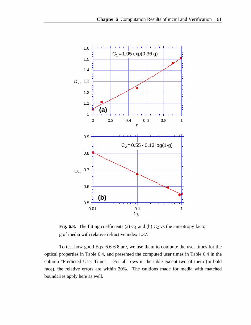
Chapter 6 Computation Results of mcml and Verification 61
1
1.1
C 1
1.2
1.3
1.4
1.5
1.6
0g
C1 = 1.05 exp(0.36 g)
0.2 0.4 0.6 0.8 1
(a)
0.5
0.6
0.7
0.8
0.9
0.01
C2 = 0.55 - 0.13 log(1-g)
C 2
0.1 1
(b)
1-g
Fig. 6.8. The fitting coefficients (a) C1 and (b) C2 vs the anisotropy factor
g of media with relative refractive index 1.37.
To test how good Eqs. 6.6-6.8 are, we use them to compute the user times for the
optical properties in Table 6.4, and presented the computed user times in Table 6.4 in the
column "Predicted User Time". For all rows in the table except two of them (in bold
face), the relative errors are within 20%. The cautions made for media with matched
boundaries apply here as well.
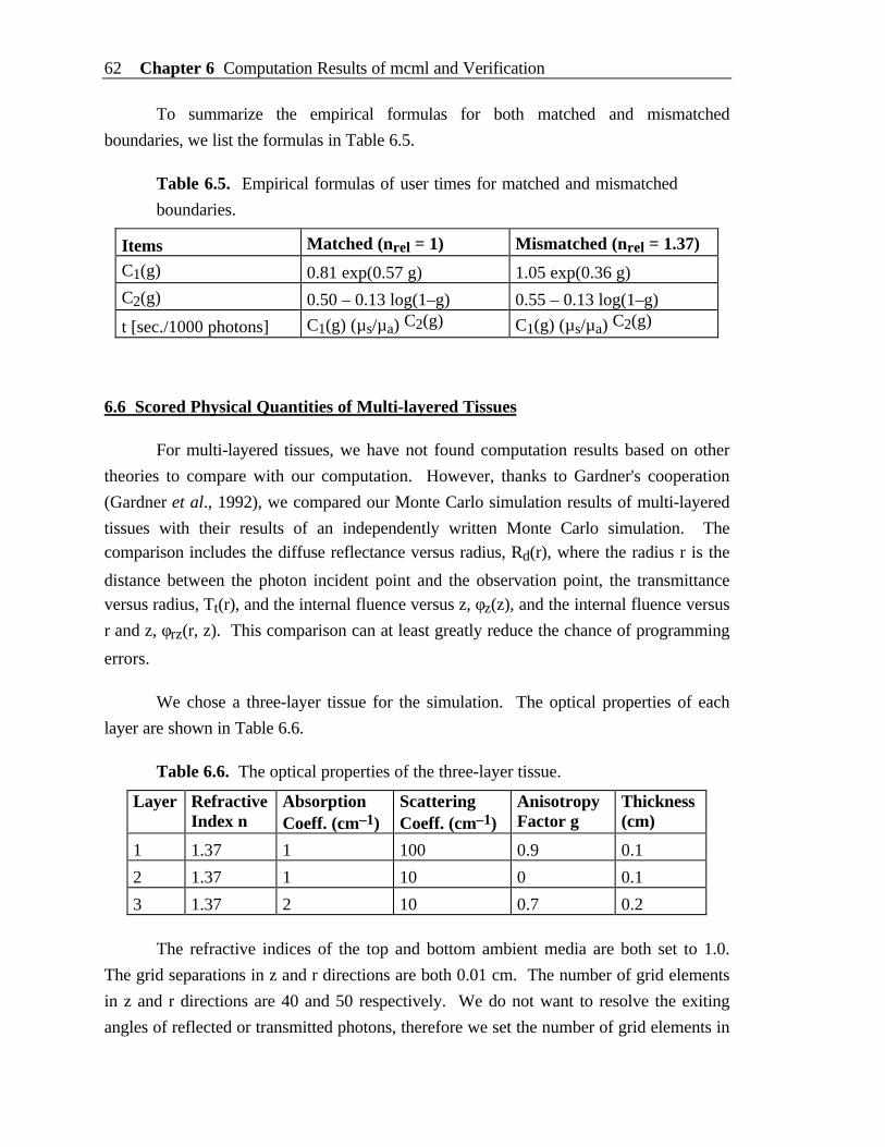
62 Chapter 6 Computation Results of mcml and Verification
To summarize the empirical formulas for both matched and mismatched
boundaries, we list the formulas in Table 6.5.
Table 6.5. Empirical formulas of user times for matched and mismatched
boundaries.
Items Matched (nrel = 1) Mismatched (nrel = 1.37)
C1(g) 0.81 exp(0.57 g) 1.05 exp(0.36 g)
C2(g) 0.50 – 0.13 log(1–g) 0.55 – 0.13 log(1–g)
t [sec./1000 photons] C1(g) (µs/µa) C2(g) C1(g) (µs/µa) C2(g)
6.6 Scored Physical Quantities of Multi-layered Tissues
For multi-layered tissues, we have not found computation results based on other
theories to compare with our computation. However, thanks to Gardner's cooperation
(Gardner et al., 1992), we compared our Monte Carlo simulation results of multi-layered
tissues with their results of an independently written Monte Carlo simulation. Thecomparison includes the diffuse reflectance versus radius, Rd(r), where the radius r is the
distance between the photon incident point and the observation point, the transmittanceversus radius, Tt(r), and the internal fluence versus z, φz(z), and the internal fluence versus
r and z, φrz(r, z). This comparison can at least greatly reduce the chance of programming
errors.
We chose a three-layer tissue for the simulation. The optical properties of each
layer are shown in Table 6.6.
Table 6.6. The optical properties of the three-layer tissue.
Layer RefractiveIndex n
AbsorptionCoeff. (cm–1)
ScatteringCoeff. (cm–1)
AnisotropyFactor g
Thickness(cm)
1 1.37 1 100 0.9 0.1
2 1.37 1 10 0 0.1
3 1.37 2 10 0.7 0.2
The refractive indices of the top and bottom ambient media are both set to 1.0.
The grid separations in z and r directions are both 0.01 cm. The number of grid elements
in z and r directions are 40 and 50 respectively. We do not want to resolve the exiting
angles of reflected or transmitted photons, therefore we set the number of grid elements in
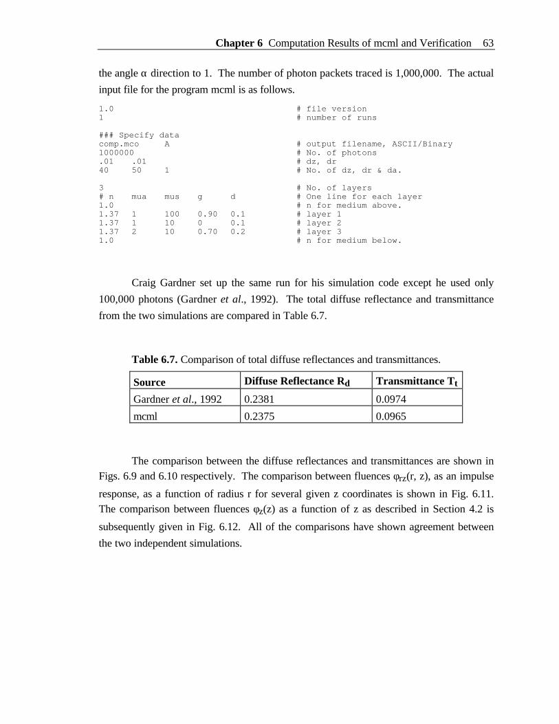
Chapter 6 Computation Results of mcml and Verification 63
the angle α direction to 1. The number of photon packets traced is 1,000,000. The actual
input file for the program mcml is as follows.
1.0 # file version1 # number of runs
### Specify datacomp.mco A # output filename, ASCII/Binary1000000 # No. of photons.01 .01 # dz, dr40 50 1 # No. of dz, dr & da.
3 # No. of layers# n mua mus g d # One line for each layer1.0 # n for medium above.1.37 1 100 0.90 0.1 # layer 11.37 1 10 0 0.1 # layer 21.37 2 10 0.70 0.2 # layer 31.0 # n for medium below.
Craig Gardner set up the same run for his simulation code except he used only
100,000 photons (Gardner et al., 1992). The total diffuse reflectance and transmittance
from the two simulations are compared in Table 6.7.
Table 6.7. Comparison of total diffuse reflectances and transmittances.
Source Diffuse Reflectance Rd Transmittance Tt
Gardner et al., 1992 0.2381 0.0974
mcml 0.2375 0.0965
The comparison between the diffuse reflectances and transmittances are shown inFigs. 6.9 and 6.10 respectively. The comparison between fluences φrz(r, z), as an impulse
response, as a function of radius r for several given z coordinates is shown in Fig. 6.11.The comparison between fluences φz(z) as a function of z as described in Section 4.2 is
subsequently given in Fig. 6.12. All of the comparisons have shown agreement between
the two independent simulations.
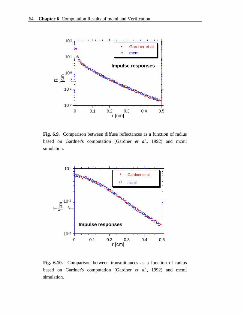
64 Chapter 6 Computation Results of mcml and Verification
10-2
10-1
10 0
10 1
10 2
R d [cm
-2 ]
0 0.1 0.2 0.3 0.4 0.5r [cm]
Gardner et al.
mcml
Impulse responses
Fig. 6.9. Comparison between diffuse reflectances as a function of radius
based on Gardner's computation (Gardner et al., 1992) and mcml
simulation.
10-2
10-1
10 0
0 0.1
T t [cm
-2 ]
0.2 0.3 0.4 0.5
Gardner et al.
mcml
r [cm]
Impulse responses
Fig. 6.10. Comparison between transmittances as a function of radius
based on Gardner's computation (Gardner et al., 1992) and mcml
simulation.
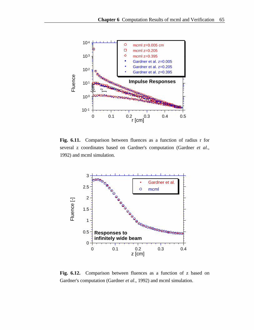
Chapter 6 Computation Results of mcml and Verification 65
10-1
10 0
10 1
10 2
10 3
10 4
Flu
ence
[cm
-2 ]
0 0.1 0.2 0.3 0.4 0.5r [cm]
mcml z=0.005 cmmcml z=0.205mcml z=0.395Gardner et al. z=0.005Gardner et al. z=0.205Gardner et al. z=0.395
Impulse Responses
Fig. 6.11. Comparison between fluences as a function of radius r for
several z coordinates based on Gardner's computation (Gardner et al.,
1992) and mcml simulation.
0
0.5
1
1.5
2
Flu
ence
[-]
2.5
3
0 0.1 0.2 0.3z [cm]
0.4
Gardner et al.
Responses to infinitely wide beam
mcml
Fig. 6.12. Comparison between fluences as a function of z based on
Gardner's computation (Gardner et al., 1992) and mcml simulation.
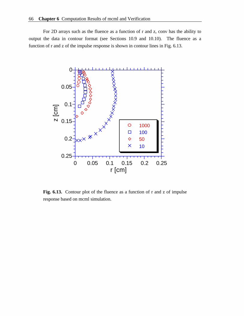
66 Chapter 6 Computation Results of mcml and Verification
For 2D arrays such as the fluence as a function of r and z, conv has the ability to
output the data in contour format (see Sections 10.9 and 10.10). The fluence as a
function of r and z of the impulse response is shown in contour lines in Fig. 6.13.
0.25
0.2
0.15
0.1
0.05
0
z [c
m]
0 0.05 0.1 0.15 0.2 0.25r [cm]
100010050
10
Fig. 6.13. Contour plot of the fluence as a function of r and z of impulse
response based on mcml simulation.
Chapter 7 Convolution for Photon Beams of Finite Size 67
7. Convolution for Photon Beams of Finite Size
This chapter will discuss the principles and implementation of convolving Monte
Carlo simulation results for an infinitely narrow photon beam to yield the responses to
photon beams of finite size. Gaussian beams and circularly flat beams are considered as
special cases.
7.1 Principles of convolution
So far we have only dealt with the response to an infinitely narrow photon beam
normally incident on the surface of a multi-layered tissue. This response is also called the
impulse response. However, all photon beams have finite size in reality. Theoretically, we
can use the Monte Carlo simulation to compute the response to a finite size photon beam
directly by distributing the initial positions of the launched photon packets. The only
problem is that it requires a larger number of photon packets to be traced to get
acceptable variance than simulating the responses of an infinitely narrow photon beam.
Therefore, this method is not efficient although sometimes it might be the only approach
for some types of tissue configurations which can not be convolved, such as a tissue with
an irregular buried object.
Fortunately, the system we are dealing with is linear and invariant. The linearity
means that if the input intensity of the infinitely narrow photon beam is multiplied by a
factor, the responses will be multiplied by the same factor. It also means that the response
to two photon beams is the sum of the responses to each photon beam. The invariance
means that when the infinitely narrow photon beam is shifted horizontally by a distance in
a certain direction, the responses will be shifted also horizontally by the same distance in
the same direction. Therefore, if we assume the photon beam of finite size is collimated,
the response of an infinitely narrow photon beam will be a Green's function of the tissue
system, and the response of the finite size photon beam can be computed from the
convolution of the Green's function according to the profile of the finite size photon beam.
Note that the responses mentioned above can be the internal absorption
distribution, or the reflectance or transmittance distributions. We denote the responses
generally as C(x, y, z) although it may not be a three-variable function of all three
coordinates. Such degeneracy due to the symmetry will be discussed subsequently. We
denote the Green's function corresponding to the type of response under consideration as
68 Chapter 7 Convolution for Photon Beams of Finite Size
G(x, y, z). Since the photon beam is normally incident on the tissue surface, the function
G(x, y, z) possesses cylindrical symmetry. If the collimated photon beam as the source has
the intensity profile S(x, y), the responses can be obtained through convolution (Prahl,
1988; Prahl et al., 1989):
C(x, y, z) = ⌡⌠–∞
∞ ⌡⌠
–∞
∞ G(x–x', y–y', z) S(x', y') dx' dy' (7.1a)
or through variable transformation with x'' = x – x' and y'' = y – y':
C(x, y, z) = ⌡⌠–∞
∞ ⌡⌠
–∞
∞ G(x'', y'', z) S(x–x'', y–y'') dx'' dy'' (7.1b)
In Eq. 7.1a the Green's function is a function of the distance between the source
point (x', y') and the observation point (x, y), where the distance is:
d' = (x–x')2 + (y–y')2 (7.2)
If the intensity profile S(x', y') of the source also has cylindrical symmetry, S(x', y') is only
a function of the radius of the source point (x', y') with respect to the origin point of the
coordinate system, where the radius is:
r' = x'2 + y'2 (7.3)
Therefore, Eq. 7.1a can be reformulated considering these symmetries:
C(x, y, z) = ⌡⌠–∞
∞ ⌡⌠
–∞
∞ G( (x–x')2 + (y–y')2 , z) S( x'2 + y'2) dx' dy' (7.4a)
Similarly, Eq. 7.1b can also be reformulated with these symmetries:
C(x, y, z) = ⌡⌠–∞
∞ ⌡⌠–∞
∞ G( x''2 + y''2 , z) S( (x–x'')2 + (y–y'')2) dx'' dy'' (7.4b)
Since the response C(x, y, z) will have the same cylindrical symmetry, the problem
can be more easily handled in a cylindrical coordinate system, where Eqs. 7.4a and 7.4b
can be written:
Chapter 7 Convolution for Photon Beams of Finite Size 69
C(r, z) = ⌡⌠
0
∞
S(r') r'
⌡⌠
0
2 π
G( )r2 + r'2 – 2rr'cosθ' , z dθ' dr' (7.5a)
C(r, z) = ⌡⌠
0
∞
G(r'', z) r''
⌡⌠
0
2 π
S( )r2 + r''2 – 2rr''cosθ'' dθ'' dr'' (7.5b)
Eq. 7.5b is more advantageous than Eq. 7.5a in computation because the integration over
θ'' is independent of z. This integration hence need only be computed once for all depths
z. In some cases as presented subsequently, the integral over θ'' can be expressed
analytically, therefore the two-dimensional integral is converted into a one dimensional
integral.
The transformation of variables is illustrated in Fig. 7.1. The first coordinate
system (r', θ', z) has its origin at the center of the source, as in Fig. 7.1A and Eq. 7.5a.
The point of observation is at (r, 0). An incremental region of source is located at (r', θ')
and has a value S(r'). The distance between the source point and the observation point is
d' equal
r2 + r'2 – 2rr'cosθ' .
The second coordinate system (r", θ", z) has its origin at the center of the point of
observation, as in Fig. 7.1B and Eq. 7.5b. The source is centered at (r, 0). The
incremental region of source is located at (r", θ") and has a value S(d"), where d" equals
r2 + r"2 – 2rr"cosθ" . The distance between the source point and the observation point
is r".
In the following sections, we will consider a Gaussian beam and a circularly flat
beam as examples of cylindrical symmetry to further simplify Eq. 7.5b.
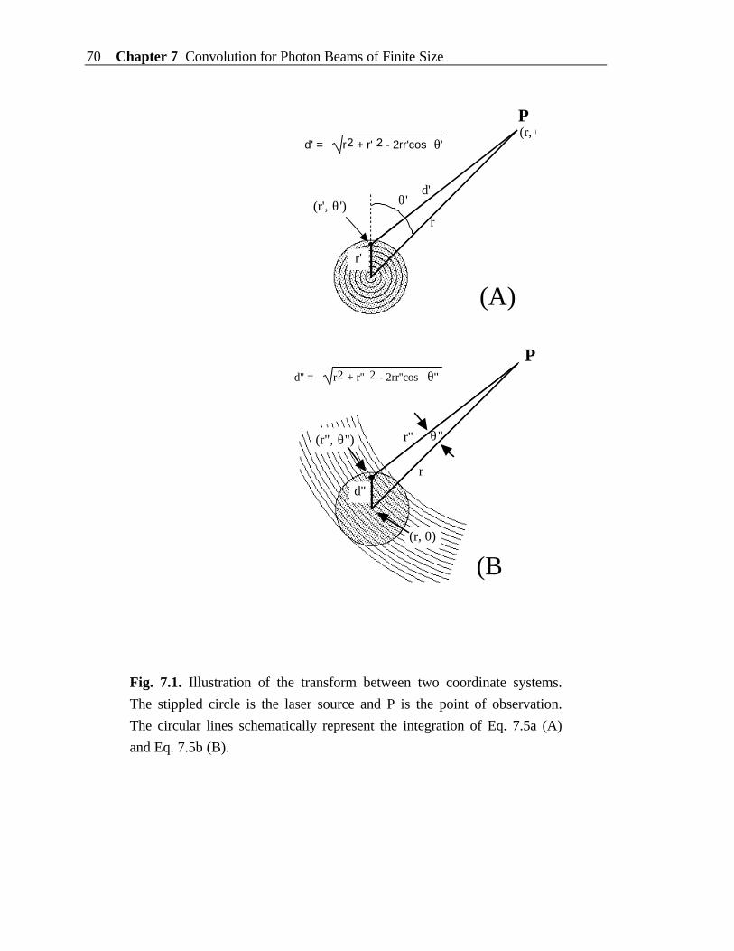
70 Chapter 7 Convolution for Photon Beams of Finite Size
Fig. 7.1. Illustration of the transform between two coordinate systems.
The stippled circle is the laser source and P is the point of observation.
The circular lines schematically represent the integration of Eq. 7.5a (A)
and Eq. 7.5b (B).
(A)
r
(r, 0)
θ"(r", θ") r"
d"
(Β)
d'
r'
r
(r, 0)
θ'(r', θ')
d'' =
r2 + r'' 2 - 2rr''cos θ''
d' =
r2 + r' 2 - 2rr'cos θ'
P
P

Chapter 7 Convolution for Photon Beams of Finite Size 71
7.2 Convolution over Gaussian beams
In the case of a Gaussian beam, if the divergence is ignored, the above convolution
can be applied. If the 1/e2 radius of the Gaussian beam is denoted by R, the beam intensity
profile is:
S(r') = S0 exp(–2 (r'/R)2) (7.6)
where the intensity in the center (r=0), S0, is related to the total power P by:
S0 = 2 P / (π R2) (7.7)
Substituting Eq. 7.6 into Eq. 7.5b, the convolution becomes:
C(r, z) = S(r)
⌡⌠
0
∞
G(r'', z)exp(–2 (r''/R)2)
⌡⌠ 0
2 π exp(4rr''cosθ''/R2) dθ'' r''dr'' (7.8)
The integration in the square brackets resembles the integral representation of the
modified Bessel function (Spiegel, 1968):
I0(x) = 1
2 π ⌡⌠ 0
2π exp(x sinθ) dθ (7.9a)
which can be reformatted to be:
I0(x) = 1
2 π ⌡⌠ 0
2π exp(x cosθ) dθ (7.9b)
Eq. 7.8 can be written by substituting Eq. 7.9b into it:
C(r, z) = S(r) ⌡⌠ 0
∞ G(r'', z) exp(–2 (r''/R)2) I0(4rr''/R2) 2 π r'' dr'' (7.10)
where I0 is the zero order modified Bessel function.

72 Chapter 7 Convolution for Photon Beams of Finite Size
7.3 Convolution over circularly flat beams
If the photon beam is homogeneous within a radius R and collimated, the source
function becomes:
S(r') = P/(π R2) if r' ≤ R 0 if r' > R (7.11)
where P is the total power of the beam. Substituting Eq. 7.11 into Eq. 7.5b, the
convolution becomes:
C(r, z) = P/(π R2) ⌡⌠ 0
∞ G(r'', z) Iθ(r, r'') 2 π r'' dr'' (7.12)
where the function Iθ(r, r'') is:
Iθ(r, r'') =
1 if R ≥ r + r''
1π cos–1((r2 + r''2 – R2)/(2rr'')) if |r – r''| ≤ R < r + r''
0 if R < |r – r''|
(7.13)
From Eq. 7.13 and Fig. 7.1B, the limits of integration in Eq. 7.12 can be changed to a
finite region:
C(r, z) = P/(π R2) ⌡⌠ a
r + R G(r'', z) Iθ(r, r'') 2 π r'' dr'' (7.14a)
where
a = Max(0, r – R) (7.14b)
where the function Max takes the larger of the two arguments.
The circular lines in Fig. 7.1B illustrated the second case in Eq. 7.13 when the
observation point P is outside of the source. When the point P is outside the source, the
first case of Eq. 7.13 is never satisfied. Readers can similarly draw the pictures for the
case where the point P is inside the source. Note that much of the region of integration
lies outside the source and therefore the value of S in the integrand is zero.
Chapter 7 Convolution for Photon Beams of Finite Size 73
As a special case of a circularly flat beam, we let the radius R approach infinity,
which represents an infinitely wide flat beam. In this case the total power P also
approaches infinity, but we can use the power density to describe the intensity of the
beam. The convolution for this case can be accomplished by simply letting R → ∞ and
P/(π R2) → S, where S is the power density or irradiance (W/cm2), in Eq. 7.14. Iθ(r, r'')
will be 1 constantly. Eq. 7.14 becomes:
C(r, z) = S ⌡⌠ 0
∞ G(r'', z) 2 π r'' dr'' (7.15)
7.4 Numerical solution to the convolution
In these two special cases of photon beams, the two-dimensional integrations are
converted into one-dimensional integrations, which are significantly faster in numerical
computation. Since the Monte Carlo simulation scores physical quantities to discrete grid
points, the best choice of integration algorithm is the extended trapezoidal rule, which is
written in C called qtrap() by Press et al. (1988). "Increased sophistication will usually
translate into a higher order method whose efficiency will greater only for sufficiently
smooth integrands. qtrap is the method of choice, e.g., for an integrand which is a
function of a variable that is linearly interpolated between measured data points." Press et
al. (1988) state.
The simplest choice of the integration is the summation of the integrand values at
the original grid points multiplied by the grid separation. However, this approach does not
have any control over the integration accuracy. For a given accuracy, sometimes this
approach gives more accuracy than required, which is a waste of computation time, and
sometimes it gives less accuracy, which does not meet the expectation. For example, the
number of original grid elements in the r direction is 50, and we want to convolve the
responses over a circularly flat beam with a radius of R which is about 5 ∆r, where ∆r is
the grid separation in the r direction. To compute C(0, z) in Eq. 7.14a, the integral range,
from 0 and R, only covers 5 ∆r. This means only 5 function evaluations will be
completed, which may yield unacceptable answer. On the contrary, the extended
trapezoidal rule does the right amount of computation until it reaches the user specified
accuracy.
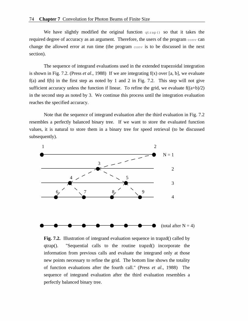
74 Chapter 7 Convolution for Photon Beams of Finite Size
We have slightly modified the original function qtrap() so that it takes the
required degree of accuracy as an argument. Therefore, the users of the program conv can
change the allowed error at run time (the program conv is to be discussed in the next
section).
The sequence of integrand evaluations used in the extended trapezoidal integration
is shown in Fig. 7.2. (Press et al., 1988) If we are integrating f(x) over [a, b], we evaluate
f(a) and f(b) in the first step as noted by 1 and 2 in Fig. 7.2. This step will not give
sufficient accuracy unless the function if linear. To refine the grid, we evaluate f((a+b)/2)
in the second step as noted by 3. We continue this process until the integration evaluation
reaches the specified accuracy.
Note that the sequence of integrand evaluation after the third evaluation in Fig. 7.2
resembles a perfectly balanced binary tree. If we want to store the evaluated function
values, it is natural to store them in a binary tree for speed retrieval (to be discussed
subsequently).
1 2
3
4 5
6 7 8 9
N = 1
2
3
4
(total after N = 4)
Fig. 7.2. Illustration of integrand evaluation sequence in trapzd() called by
qtrap(). "Sequential calls to the routine trapzd() incorporate the
information from previous calls and evaluate the integrand only at those
new points necessary to refine the grid. The bottom line shows the totality
of function evaluations after the fourth call." (Press et al., 1988) The
sequence of integrand evaluation after the third evaluation resembles a
perfectly balanced binary tree.
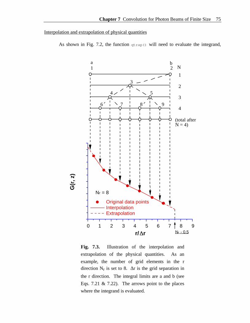
Chapter 7 Convolution for Photon Beams of Finite Size 75
Interpolation and extrapolation of physical quantities
As shown in Fig. 7.2, the function qtrap() will need to evaluate the integrand,
Original data pointsInterpolationExtrapolation
Nr = 8
G(r
, z)
0 1 2 3 4 5 6
r/ ∆∆r7 8 9
Nr - 0.5
1 21
2
3
4
(total after N = 4)
N
3
4 5
6 7 8 9
a b
Fig. 7.3. Illustration of the interpolation and
extrapolation of the physical quantities. As an
example, the number of grid elements in the rdirection Nr is set to 8. ∆r is the grid separation in
the r direction. The integral limits are a and b (see
Eqs. 7.21 & 7.22). The arrows point to the places
where the integrand is evaluated.
76 Chapter 7 Convolution for Photon Beams of Finite Size
hence the physical quantities, at points which may not be the original grid points. Linear
interpolations are used for those points that fall between two original grid points. Linear
extrapolations are used for those points that fall beyond the original grid system. The
interpolation and extrapolation are illustrated in Fig. 7.3. The solid circles represent the
original score values at the grid points. The solid lines and the dashed lines represent the
interpolation and extrapolation respectively. For a given number of grid elements in the rdirection (e.g., Nr = 8 in this picture), the extrapolation is only computed up to (Nr - 0.5)
because the linear extrapolation can be unreliable for points beyond (Nr - 0.5). Therefore,
the physical quantity is set to zero beyond (Nr - 0.5). Sometimes, the data may be so
noisy that the function at the last point is even higher than the function at the second to the
last point. In this case, the extrapolation is not used. Instead, we simply set the function
values to zero. Note that as we mentioned in the beginning of Chapter 4, the last cells in
the r direction are used to collect the photons that do not fit into the grid system.
Therefore, the values in the last cell are usually much higher than the values in the second
to the last cells, and hence are not used in the convolution process. In a word, thephysical quantities are non-zero in the interval [0, rmax], where rmax is:
rmax = (Nr – 0.5) ∆r (7.16)
where ∆r is the grid separation in the r direction.
Integrand evaluation for Gaussian beams
As shown in Eq. 7.10, the evaluation of the physical quantities is only part of the
integrand evaluation for convolution over the Gaussian beam. Although the integration
has to converge due to physical reasons, the form of Eq. 7.10 may not be directly
computed numerically because the modified Bessel function increases rapidly as the
argument increases, and it can exceed the limit which the computer can hold (e.g., 10+38
for some computers). Therefore, a proper reformulation is required to compute Eq. 7.10.
We note that the modified Bessel function in the region where the argument is large has
the following approximation:
I0(x) ≈ exp(x) / 2 π x for large x (7.17)
Therefore, if we extract the exponential term from I0(), we can make sure the modified
Bessel function decreases as the argument increases. We define the following newfunction based on I0():
Chapter 7 Convolution for Photon Beams of Finite Size 77
I0e(x) = I0(x) exp(–x) (7.18a)
or
I0(x) = I0e(x) exp(x) (7.18b)
I0e() should always be bounded. Note that Eq. 7.17 is presented just to show the
asymptotic behavior of the function I0(). Eq. 7.18a by no means carries any
approximations. Substituting Eqs. 7.6, 7.7 and 7.18b into Eq. 7.10, it becomes:
C(r, z) = 4 PR2 ⌡
⌠
0
∞
G(r'', z) exp[–2 (r''– r R )2] I0e(
4rr''R2 ) r'' dr'' (7.19)
Since both the exponential term and the I0e() term decrease, the integrand can be
computed without being out of bound.
Up to now, we have just solved the problem of how to compute the convolution
without overflow. However, the computation speed is another issue. We found that theevaluation of the exp() I0e() in Eq. 7.19 is a major part of the computation for each
integration, which can be up to 90% depending on the specific problem being solved. For
multi-variant physical quantities (e.g., A(r, z)), the convolution may repeatedly evaluatethe exp() I0e() in Eq. 7.19 at the same point as the integration is computed for different z
coordinates.
Therefore, if we can save the function evaluations, i.e. the computations ofexp() I0e() in Eq. 7.19, for one z coordinate, then we can save a lot computation time.
However, the integration is executed iteratively until a given precision is reached. Hence,
the number of function evaluations is unknown in advance. We can only save the function
evaluations with dynamic data allocation. Furthermore, since the evaluation sequence of
the trapezoidal integration qtrap() resembles a binary tree as in Fig. 7.2., a well-balanced
binary tree can be used to store the function evaluations for searching speed.
Integral Limits for Gaussian beams
Since the integral limits in Eq. 7.14a for circularly flat beams are finite, the
integration can be computed directly using the function qtrap(). In contrast, the upper
integral limit in Eq. 7.19 for Gaussian beams is infinity. This problem can be solved using
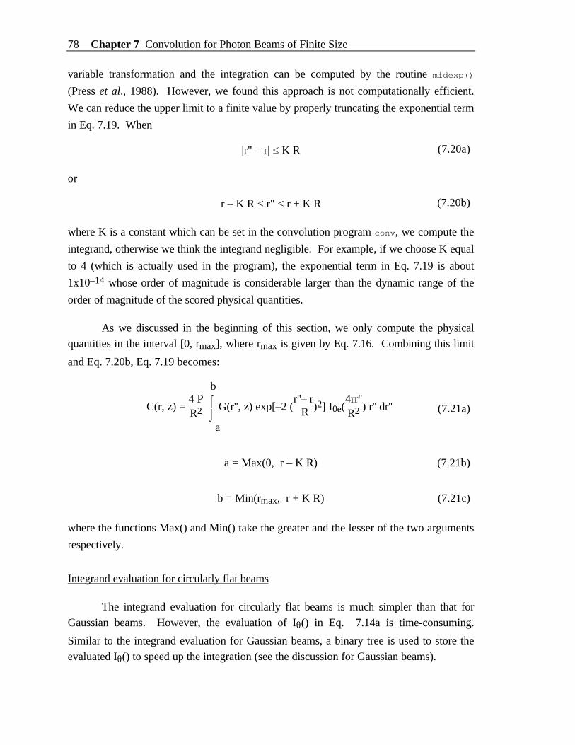
78 Chapter 7 Convolution for Photon Beams of Finite Size
variable transformation and the integration can be computed by the routine midexp()
(Press et al., 1988). However, we found this approach is not computationally efficient.
We can reduce the upper limit to a finite value by properly truncating the exponential term
in Eq. 7.19. When
|r" – r| ≤ K R (7.20a)
or
r – K R ≤ r" ≤ r + K R (7.20b)
where K is a constant which can be set in the convolution program conv, we compute the
integrand, otherwise we think the integrand negligible. For example, if we choose K equal
to 4 (which is actually used in the program), the exponential term in Eq. 7.19 is about
1x10–14 whose order of magnitude is considerable larger than the dynamic range of the
order of magnitude of the scored physical quantities.
As we discussed in the beginning of this section, we only compute the physicalquantities in the interval [0, rmax], where rmax is given by Eq. 7.16. Combining this limit
and Eq. 7.20b, Eq. 7.19 becomes:
C(r, z) = 4 PR2 ⌡
⌠
a
b
G(r'', z) exp[–2 (r''– r R )2] I0e(
4rr''R2 ) r'' dr'' (7.21a)
a = Max(0, r – K R) (7.21b)
b = Min(rmax, r + K R) (7.21c)
where the functions Max() and Min() take the greater and the lesser of the two arguments
respectively.
Integrand evaluation for circularly flat beams
The integrand evaluation for circularly flat beams is much simpler than that for
Gaussian beams. However, the evaluation of Iθ() in Eq. 7.14a is time-consuming.
Similar to the integrand evaluation for Gaussian beams, a binary tree is used to store the
evaluated Iθ() to speed up the integration (see the discussion for Gaussian beams).

Chapter 7 Convolution for Photon Beams of Finite Size 79
Integral Limits for circularly flat beams
Since the integral limits in Eq. 7.14a for circularly flat beams are finite, the
integration can be computed directly using the function qtrap(). As we discussed in thebeginning of this section, we only compute the physical quantities in the interval [0, rmax],
where rmax is given by Eq. 7.16. Considering this limit, Eq. 7.14a becomes:
C(r, z) = P/(π R2) ⌡⌠ a
b G(r'', z) Iθ(r, r'') 2 π r'' dr'' (7.22a)
a = Max(0, r – R) (7.22b)
b = Min(rmax, r + R) (7.22c)
where the functions Max() and Min() take the greater and the lesser of the two arguments
respectively.
Source of error in convolution
In Eqs. 7.21c and 7.22c, the upper limit of the integration may be limited by rmax
which is the grid limit in the r direction during the Monte Carlo simulation. The physical
quantities beyond the original grid limit in the r direction do not contribute to the
convolution, which leads an error.
Let us discuss the case for circularly flat beams first because it is easier. From Eq.
7.22c, we know that when
rmax ≥ r + R (7.23a)
or
r ≤ rmax – R (7.23b)
the limited grid in the r direction does not affect the convolution. Otherwise, the
convolution is truncated by the limited grid in the r direction. This effect can be see in thenext section. Therefore, we should not trust the convolution data for r ≥ rmax – R. In
other words, if you want to observe the physical quantity at r in response to a circularly

80 Chapter 7 Convolution for Photon Beams of Finite Size
flat beam of radius R, the grid limit in the r direction should be large enough so that Eq.
7.23a holds when you perform the Monte Carlo simulation with mcml.
For Gaussian beams, there are no clean formulas like Eqs. 7.23 to describe the
valid range because the Gaussian beams theoretically extend to infinity in the r direction.
However, the convolution results of a Gaussian beam with a 1/e2 radius of R is so close
to those of a circularly flat beam with a radius of R for r >> R (shown in the next section).
Therefore, we can use the same criteria for circularly flat beams (Eqs. 7.23) for Gaussian
beams to certain precision.
The other source of error is due to the Monte Carlo simulation by mcml 1.0. This
version of mcml does not score the first interactions separately (see Section 4.3) as
Gardner et al. (1992b) did. This may make considerable error if the radius of the
Gaussian beam is less than three times the grid separation ∆r. In other words, the
following equation should be satisfied to get reliable convolution:
R ≥ 3 ∆r (7.24)
In summary, when Eqs. 7.23 and 7.24 hold, the convolution should be reliable.
7.5 Computation results of conv and verification
The convolution process of the Monte Carlo simulation results from mcml is
implemented in another program called "conv". Like the program mcml, it is written in
ANSI Standard C, hence it can be executed on a variety of computers.
Convolution results of Gaussian beams
We do not have any standard data to verify the convolution program. However,
Craig Gardner kindly provided some convolution results using his convolution program
(Gardner et al., 1992). The impulse responses are based on the simulation discussed in
Section 6.6 where we have used the same turbid media and grid system. He computed his
convolution on his Monte Carlo simulation results, and we did it on ours after we
compared the Monte Carlo simulation results in Section 6.6.
The incident photon beam is a Gaussian beam with total energy of 1 J and radius of
0.1 cm. The convolved diffuse reflectances and transmittance are compared in Figs. 7.4
and 7.5 respectively. The convolved fluences are compared in Fig. 7.6. Note that the
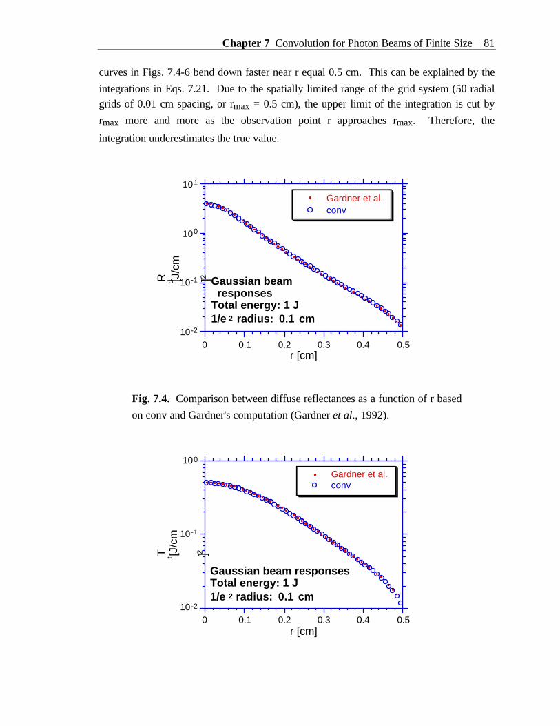
Chapter 7 Convolution for Photon Beams of Finite Size 81
curves in Figs. 7.4-6 bend down faster near r equal 0.5 cm. This can be explained by the
integrations in Eqs. 7.21. Due to the spatially limited range of the grid system (50 radialgrids of 0.01 cm spacing, or rmax = 0.5 cm), the upper limit of the integration is cut by
rmax more and more as the observation point r approaches rmax. Therefore, the
integration underestimates the true value.
10 -2
10 -1
100
101
0
R d [J/c
m
2 ]
0.1 0.2 0.3 0.4 0.5
Gardner et al.
r [cm]
conv
Gaussian beam responsesTotal energy: 1 J1/e 2 radius: 0.1 cm
Fig. 7.4. Comparison between diffuse reflectances as a function of r based
on conv and Gardner's computation (Gardner et al., 1992).
10 -2
10 -1
100
0 0.1
T t [J/c
m
2 ]
0.2 0.3 0.4 0.5
Gardner et al.conv
r [cm]
Gaussian beam responsesTotal energy: 1 J1/e 2 radius: 0.1 cm
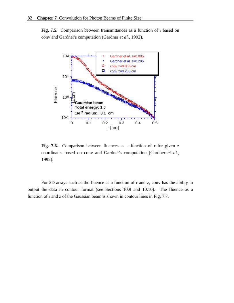
82 Chapter 7 Convolution for Photon Beams of Finite Size
Fig. 7.5. Comparison between transmittances as a function of r based on
conv and Gardner's computation (Gardner et al., 1992).
10 -1
100
101
102
0
Flu
ence
[J/c
m
2 ]
0.1 0.2 0.3 0.4 0.5
Gardner et al. z=0.005
r [cm]
Gardner et al. z=0.205
conv z=0.005 cm
conv z=0.205 cm
Gaussian beamTotal energy: 1 J
1/e 2 radius: 0.1 cm
Fig. 7.6. Comparison between fluences as a function of r for given z
coordinates based on conv and Gardner's computation (Gardner et al.,
1992).
For 2D arrays such as the fluence as a function of r and z, conv has the ability to
output the data in contour format (see Sections 10.9 and 10.10). The fluence as a
function of r and z of the Gaussian beam is shown in contour lines in Fig. 7.7.
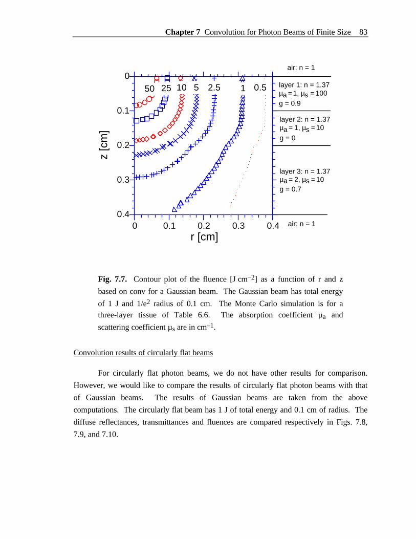
Chapter 7 Convolution for Photon Beams of Finite Size 83
0.4
0.3
0.2
0.1
0
0 0.1
z [c
m]
0.2 0.3 0.4
air: n = 1
layer 1: n = 1.37µa = 1, µs = 100
g = 0.9
layer 2: n = 1.37µa = 1, µs = 10
g = 0
r [cm]
layer 3: n = 1.37µa = 2, µs = 10g = 0.7
air: n = 1
50 25 10 5 2.5 1 0.5
Fig. 7.7. Contour plot of the fluence [J cm−2] as a function of r and z
based on conv for a Gaussian beam. The Gaussian beam has total energy
of 1 J and 1/e2 radius of 0.1 cm. The Monte Carlo simulation is for athree-layer tissue of Table 6.6. The absorption coefficient µa and
scattering coefficient µs are in cm–1.
Convolution results of circularly flat beams
For circularly flat photon beams, we do not have other results for comparison.
However, we would like to compare the results of circularly flat photon beams with that
of Gaussian beams. The results of Gaussian beams are taken from the above
computations. The circularly flat beam has 1 J of total energy and 0.1 cm of radius. The
diffuse reflectances, transmittances and fluences are compared respectively in Figs. 7.8,
7.9, and 7.10.
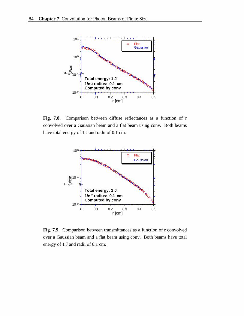
84 Chapter 7 Convolution for Photon Beams of Finite Size
10 -2
10 -1
100
101
0
R d [J/c
m
2 ]
0.1 0.2 0.3 0.4 0.5
Flat
r [cm]
Gaussian
Total energy: 1 J1/e 2 radius: 0.1 cmComputed by conv
Fig. 7.8. Comparison between diffuse reflectances as a function of r
convolved over a Gaussian beam and a flat beam using conv. Both beams
have total energy of 1 J and radii of 0.1 cm.
10 -2
10 -1
100
0 0.1
T t [J/c
m
2 ]
0.2 0.3 0.4 0.5
FlatGaussian
r [cm]
Total energy: 1 J1/e 2 radius: 0.1 cmComputed by conv
Fig. 7.9. Comparison between transmittances as a function of r convolved
over a Gaussian beam and a flat beam using conv. Both beams have total
energy of 1 J and radii of 0.1 cm.
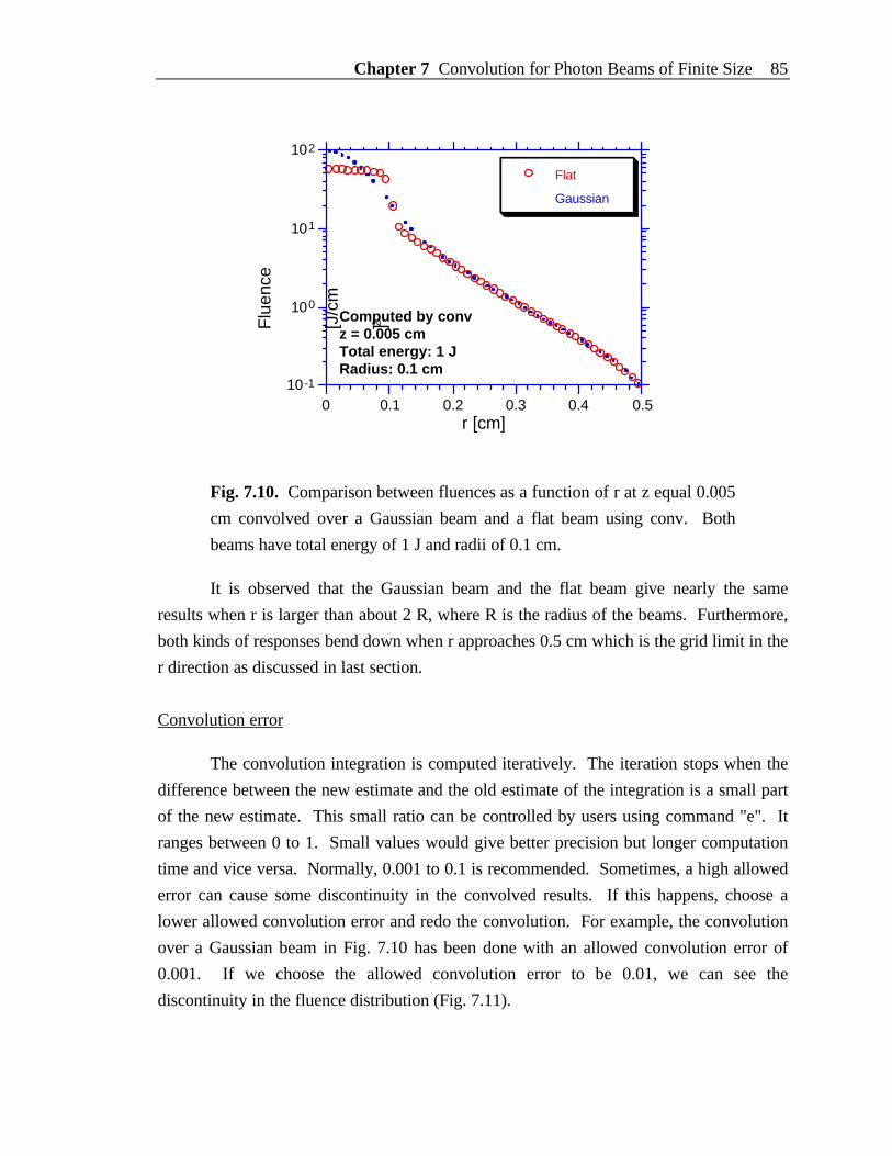
Chapter 7 Convolution for Photon Beams of Finite Size 85
10 -1
100
101
102
0
Flu
ence
[J/c
m
2 ]0.1 0.2 0.3 0.4 0.5
Flat
r [cm]
Gaussian
Computed by convz = 0.005 cmTotal energy: 1 JRadius: 0.1 cm
Fig. 7.10. Comparison between fluences as a function of r at z equal 0.005
cm convolved over a Gaussian beam and a flat beam using conv. Both
beams have total energy of 1 J and radii of 0.1 cm.
It is observed that the Gaussian beam and the flat beam give nearly the same
results when r is larger than about 2 R, where R is the radius of the beams. Furthermore,
both kinds of responses bend down when r approaches 0.5 cm which is the grid limit in the
r direction as discussed in last section.
Convolution error
The convolution integration is computed iteratively. The iteration stops when the
difference between the new estimate and the old estimate of the integration is a small part
of the new estimate. This small ratio can be controlled by users using command "e". It
ranges between 0 to 1. Small values would give better precision but longer computation
time and vice versa. Normally, 0.001 to 0.1 is recommended. Sometimes, a high allowed
error can cause some discontinuity in the convolved results. If this happens, choose a
lower allowed convolution error and redo the convolution. For example, the convolution
over a Gaussian beam in Fig. 7.10 has been done with an allowed convolution error of
0.001. If we choose the allowed convolution error to be 0.01, we can see the
discontinuity in the fluence distribution (Fig. 7.11).
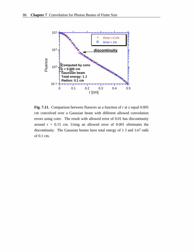
86 Chapter 7 Convolution for Photon Beams of Finite Size
10 -1
100
101
102
0
Flu
ence
[J/c
m
2 ]
0.1 0.2 0.3 0.4 0.5
Error = 0.1%
r [cm]
Error = 1%
discontinuity
Computed by convz = 0.005 cmGaussian beamTotal energy: 1 JRadius: 0.1 cm
Fig. 7.11. Comparison between fluences as a function of r at z equal 0.005
cm convolved over a Gaussian beam with different allowed convolution
errors using conv. The result with allowed error of 0.01 has discontinuity
around r = 0.15 cm. Using an allowed error of 0.001 eliminates the
discontinuity. The Gaussian beams have total energy of 1 J and 1/e2 radii
of 0.1 cm.
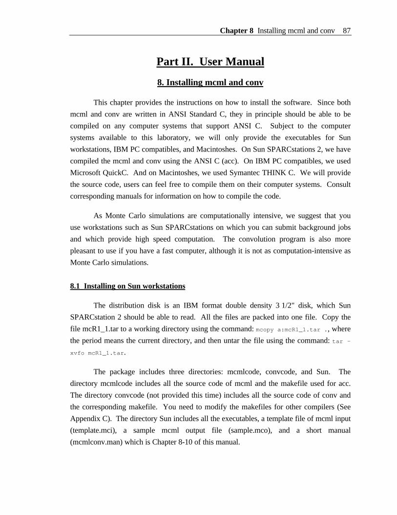
Chapter 8 Installing mcml and conv 87
Part II. User Manual
8. Installing mcml and conv
This chapter provides the instructions on how to install the software. Since both
mcml and conv are written in ANSI Standard C, they in principle should be able to be
compiled on any computer systems that support ANSI C. Subject to the computer
systems available to this laboratory, we will only provide the executables for Sun
workstations, IBM PC compatibles, and Macintoshes. On Sun SPARCstations 2, we have
compiled the mcml and conv using the ANSI C (acc). On IBM PC compatibles, we used
Microsoft QuickC. And on Macintoshes, we used Symantec THINK C. We will provide
the source code, users can feel free to compile them on their computer systems. Consult
corresponding manuals for information on how to compile the code.
As Monte Carlo simulations are computationally intensive, we suggest that you
use workstations such as Sun SPARCstations on which you can submit background jobs
and which provide high speed computation. The convolution program is also more
pleasant to use if you have a fast computer, although it is not as computation-intensive as
Monte Carlo simulations.
8.1 Installing on Sun workstations
The distribution disk is an IBM format double density 3 1/2" disk, which Sun
SPARCstation 2 should be able to read. All the files are packed into one file. Copy the
file mcR1_1.tar to a working directory using the command: mcopy a:mcR1_1.tar ., where
the period means the current directory, and then untar the file using the command: tar -
xvfo mcR1_1.tar.
The package includes three directories: mcmlcode, convcode, and Sun. The
directory mcmlcode includes all the source code of mcml and the makefile used for acc.
The directory convcode (not provided this time) includes all the source code of conv and
the corresponding makefile. You need to modify the makefiles for other compilers (See
Appendix C). The directory Sun includes all the executables, a template file of mcml input
(template.mci), a sample mcml output file (sample.mco), and a short manual
(mcmlconv.man) which is Chapter 8-10 of this manual.

88 Chapter 8 Installing mcml and conv
To install the executables, copy the executables to the sub directory ~/bin under
your home directory. Then, put the directory ~/bin under the search path in .cshrc or
.login if you are using C Shell. Consult manual if you are using other shells.
Having finished copying, you can eject the disk using the command eject. If your
Sun workstation does not have a floppy drive, you can transfer the files through a
networked IBM PC or a compatible. If you have an electronic mail address, we can also
send the package to you through mail.
8.2 Installing on IBM PC compatibles
For IBM PC's or compatibles, the distribution disk is a double density 3 1/2" disk.
An alternative 5 1/4" disk can be sent upon request. All the files are packed into one file.
Copy the self-extracting file mcR1_1.exe to your working directory on your hard drive
and run the file to extract all packed files using the command: mcR1_1.exe -d, where the
option "-d" keeps the directory structure.
The package includes three directories: mcmlcode, convcode, and IBMPC. The
directory mcmlcode includes all the source code of mcml. The directory convcode (not
provided for now) includes all the source code of conv. The directory IBMPC includes all
the executables, a template file of mcml input (template.mci), a sample mcml output file
(sample.mco), and a short manual (mcmlconv.man) which is Chapter 8-10 of this manual.
The executables include mcml.exe and conv.exe. The code was compiled and linked using
Microsoft QuickC 2.5. The executables will be able to detect whether your computer has
math coprocessor, and take advantage of the math coprocessors if they are present.
If you want to be able to execute the programs under any directory, you should
put the directory IBMPC in the search path. The search path can be changed in the file
autoexec.bat.
8.3 Installing on Macintoshes
For Macintoshes, the distribution disk is a double density 3 1/2" disk. All the files
are packed into one file. Copy the self-extracting file mcR1.1.sea to a working folder on
you hard drive, and double click on the icon to extract the files.
The package includes three folders: mcmlcode, convcode, and Mac. The folder
mcmlcode includes all the source code of mcml. The folder convcode includes all the

Chapter 8 Installing mcml and conv 89
source code of conv. The folder Mac includes all the executables, a template file of mcml
input (template.mci), a sample mcml output file (sample.mco), and a short manual
(mcmlconv.man) which is Chapter 8-10 of this manual. The executables include
mcml.fpu, conv.fpu, mcml.020, conv.020, mcml.000, and conv.000 for different types of
computers as discussed subsequently.
Before you install the executables, you need to know what kind of Macintosh you
are using. You can test the following conditions to decide which executables to use:
A. MC68040
B. MC68020 or MC68030
C. MC68881 or MC68882
If your Macintosh meets condition A, or conditions B and C, you should copy the
executables with extensions ".fpu". If your Macintosh meets condition B only, you should
keep the executables with extensions ".020". Otherwise, you should use the executables
with extensions ".000". We suggest that you remove the extensions of the executables on
your hard drive to keep consistency with the manual.
8.4 Installing by Electronic Mail
For these users who have electronic mail access on UNIX machines, we can
deliver the software package through electronic mails. The package is archived using the
command tar, compressed using the command compress, then encoded using the
command uuencode before it is mailed out using the mail utilities. After you receive the
mail, you need to do the following.
1. Save the mail as a file, e.g., mc.mail.
2. Decode the file (mc.mail) to get a file named mc.tar.Z using
uudecode mc.mail
3. Uncompress the file mc.tar.Z to get the file mc.tar
uncompress mc.tar.Z
4. Unarchive the file mc.tar to get the package using:

90 Chapter 8 Installing mcml and conv
tar -xvfo mc.tar
At this moment, you should have three directories under the working directory. They are
mcmlcode, convcode, and Sun, or IBMPC, or Mac.
If you ordered a Sun version of the package, you only need to put the executables
under the proper directory., e.g., ~/bin (see Section 8.1).
If you ordered an IBM PC version or a Mac version of the package, you need to
transfer the files to your local computer using FTP or modem. Then refer to Section 8.2
or 8.3 for details.
It is appropriate to describe in more detail how we send the package through
electronic mails which is exactly the opposite of the above procedure. We put the
package in a working directory which include three subdirectories: mcmlcode, convcode,
and Sun, or IBMPC, or Mac. Then:
tar -cvf mc.tar
compress mc.tar
uuencode mc.tar.Z mc.tar.Z > mc.mail
mail your_address
In the mail utility, you can add in any messages in the beginning of the mail, then you need
to use the command r to read in the file mc.mail. Then, you can send the file by typing a
period "." and a return in a new line (see the manual page of mail).
Chapter 9 Instructions for mcml 91
9. Instructions for mcml
This chapter describes the actual instructions to use mcml. Macintoshes, IBM PC
compatibles and UNIX machines are used as examples of computer systems, although
mcml can execute on any computer systems that support ANSI Standard C. The reader is
assumed to be familiar with the operating system and comfortable with at least one of the
text editors on the computer system to be used to execute mcml. Three steps involved in
the Monte Carlo simulation using mcml are included in the following sections: preparing
the input data file, executing the program mcml with the input data file, processing the
output data in the data files named in the input data file. We will also show some known
bugs.
9.1 File of input data
The first step to do the simulation using mcml is to prepare an input data file (e.g.,
"filename.mci"). Any valid filenames on your system without spaces will be acceptable,
but extension ".mci" is recommended. In ANSI C, spaces are used as separators.
Therefore, filenames with spaces may not be accepted by mcml, although they are allowed
by some operating systems themselves such as the Macintosh System. We will use
"filename.mci" as an example in the following discussions.
This input data file may be edited with any text editors such as Apple Edit,
MockWrite or Microsoft Word on Macintoshes, Norton editor NE or Microsoft Word on
IBM PC compatibles, vi editor or EMACS on UNIX systems. However, if you use word
processors like Microsoft Word to edit the file, make sure that you save the file in text
format since mcml does not accept binary files as input. If you are using the UNIX system
and are uncomfortable with vi or other editors available on UNIX, you can use editors on
your personal computer, then transfer the file using Kermit if you use modem or FTP if
your personal computer is on a network. Make sure to use ASCII or text mode when you
transfer this file.
The best way to write an input data file is to make a copy of the template file
called "template.mci" (See Appendix D), then modify the parameters in the file. The input
data file is organized line by line. All parameters must be in the right order. The lines with
parameters in order must also be in order themselves. However, feel free to insert
comment lines or space lines in between to make the file more readable. Comment lines

92 Chapter 9 Instructions for mcml
start with the symbol "#". The symbol "#" can also be used after the parameters in a line
to mark the start of comments.
The parameters in the input data file are read by mcml line by line. If there are
multiple parameters in a line, use tabs or spaces to separate them. A tab is preferred,
because it aligns the parameters for better readability. All dimensional quantities are in cm
or derived from cm. The thickness of each layer is in cm. The grid line separations are
also in cm. Absorption coefficient and scattering coefficient are in 1/cm. Each line of the
input file is explained in the order that they appear in the input data file as follows.
1. File version of the input data file. Always use "1.0" for now.
2. Number of runs (integer). Each run is an independent simulation. You can specify
any number of runs, which is not subject to memory limit. Make sure you use an
integer instead of a floating point number for this parameter, e.g., 5 instead of 5.0.
3. Output filename and file format. Extension ".mco" is recommended for the output
filenames, e.g., "output1.mco". The program mcml currently only supports ASCII
format, therefore always use "A" as the second parameter in this line. Make sure
that you use different output filenames if you have multiple runs in an input data
file, although mcml checks for this mistake. What is more important is that the
filenames should not be the same as the names of existent ones unless you want to
overwrite the existent files on purpose. Since the program mcml does not check
this error, you will lose the existent files.
4. Number of photon packets to be traced (integer).
5. Separations (in cm) between grid lines in z and r direction of the cylindrical
coordinate system. These are floating point numbers. Both z and r originate from
the photon incident point on the surface of first layer, and the z axis points down
into the turbid medium. Make sure these parameters are large enough to give you
an acceptable variance, and small enough to give you an acceptable resolution.
These parameters should be determined coordinately with the number of photons
to achieve both accuracy and resolution. Also note that users should try to choose
grid size in the z direction so that grid boxes do not cross tissue-tissue interfaces
or boundaries (see Section 9.5).

Chapter 9 Instructions for mcml 93
6. Number of grid elements (integers) in the z, r directions of the cylindrical
coordinate system and in the alpha direction, where alpha is the angle spanned
between the photon exiting direction and the surface normal. Since the angle
always covers 0 through 90 degrees, the angular separation is 90 degrees divided
by the number of angular grid elements specified in this line. Be careful with this
line, if the numbers are too large, the output file will be very big because 2D arrays
are written into the output file. If you do not need to resolve one of the directions
(z or r) or the angle, use 1 (not 0) for that parameter. Make sure to use integers
for these three parameters.
7. Number of layers (integer). This number does not include the ambient media above
or below the tissue.
8. Refractive index for the top ambient medium above the first layer (e.g., 1.0 for
air).
9. Layer parameter lines. One line for each layer. In each line are the refractive
index, the absorption coefficient (1/cm), the scattering coefficient (1/cm), the
anisotropy factor, and the thickness (cm). To simulate semi-infinite tissue, use a
very large thickness (e.g., 1E8 cm) compared with the mean free path of the tissue.
10. Refractive index for the bottom ambient medium below the last layer (e.g., 1.0 for
air).
11. Repeat lines 3 through 10 for each additional run if you have multiple runs.
Note: Two points are worth noting. The only limit to the number of grid elements
and layers is the amount of memory allocated to mcml in your system because the arrays
are dynamically allocated according to these parameters. Do not use floating point
numbers for the integers. Otherwise, the program may interpret them incorrectly.
However, you may use integers for floating point numbers, e.g., 100 instead of 100.0.
9.2 Execution
Once the input data file is prepared, the program mcml can be executed using the
input data file. During the execution, the program mcml will report an output message
which gives the number of photons remaining in the simulation, the number of runs left,
and the time of ending the job. The first report is after 10 photon packets are traced, then

94 Chapter 9 Instructions for mcml
it is updated when every 1/10 of the total number of photon packets are traced. The
methods of execution are slightly different on different operating systems.
Macintosh
To run mcml on Macintosh System 6, you have to copy or move the executable
mcml to your working folder where the input data file resides, then double click on the
mcml icon to start the program. The program mcml will prompt for the input data
filename, which is entered through the keyboard. If the input data file cannot be found,
the program will prompt you again until it finds the file or a period "." is typed, where "."
is used to abort the program. If you use Macintosh System 7, you may use an alias of
mcml instead of a copy of it.
IBM PC compatibles
For IBM PC compatibles, make sure that the directory with mcml is in the search
path, which can be checked by typing the command "path" or the file "autoexec.bat". To
run mcml with the input data file as a command parameter under DOS command prompt,
type:
mcml filename.mci
If you want to save the output message as a file (e.g., message.out), type:
mcml filename.mci > message.out
which redirects the output message to the file "message.out". To run mcml in the
interactive mode, type the following command without input data filename:
mcml
Then, the program mcml will prompt for the input data file.
UNIX
On a UNIX system, you should place the executable mcml in a directory that is in
the search path. The directory ~/bin is a good choice. The search path can be found and
modified in the file ".cshrc" if you are using C Shell or the file ".login". The three ways of
Chapter 9 Instructions for mcml 95
invoking mcml under DOS can be used under UNIX operating systems. Moreover, if you
wish to discard the messages during the execution, use the command:
mcml filename.mci > /dev/null
which redirects the output to the "bit bucket" (/dev/null). You can also simply submit a
background job using:
mcml filename.mci > /dev/null &
Refer to your UNIX manual for how to inquire about the status of a background
job. If you are still in the same session, the command "jobs" can be used in C Shell.
Otherwise, you should use the UNIX command "ps" to check for background processes.
You can also directly look for the output files to check if the job is done.
9.3 File of output data
When the job is completed, the results will be written into the output data files as
you named in your input data file. A sample output data file is shown in Appendix E. The
output data files can be read with any text editors if they are ASCII as a result of using
"A" for the file format in the input data file. They may be big if your numbers of grid
elements are large.
The contents of output files are self explanatory. The same policy for the input
data file is used for the output data file, that is, comment lines starting with a symbol "#"
and space lines are written to the file for clarity. The first line is used for file type
identification when the file is read by other applications. Then, the user time spent on the
simulation is reported in a comment line. Then, a few categories of data are reported
sequentially in the following order: pure numbers, 1D arrays and 2D arrays. The
definitions of the output data can be found in Chapter 4. The category "InParm" reports
all the input parameters specified in the input data file again so that the output file is a
complete reference and the input parameters may also be double checked against any
errors in the input data file. The category "RAT" reports the specular reflectance, the
total diffuse reflectance, the total absorption, and the total transmittance. The category
"A_l" is the absorption as a function of layer. The category "A_z" is the absorption as a
function of depth z. The categories "Rd_r" and "Rd_a" are the diffuse reflectances as a
function of radius r and angle alpha respectively. The categories "Tt_r" and "Tt_a" are the
transmittance as a function of radius r and angle alpha respectively. The 2D arrays A_rz,
96 Chapter 9 Instructions for mcml
Rd_ra, and Tt_ra are then reported. The category A_rz is the absorption as a function of
depth z and radius r. The categories Rd_ra and Tt_ra are correspondingly the diffuse
reflectance and transmittance as a function of radius r and angle alpha. The name of each
category is written before the data, such that the data can be easily identified. The units
for these data were discussed in Chapter 4.
9.4 Subset of output data
Sometimes, only a subset of the output data is needed for presentation or
processing. For example, we may need to print a 1D array into a file in XY format,
namely two columns of data, or a 2D array in XYZ format. These files can then be read
into some commercial applications such as AXUM on IBM PC compatibles and
KaleidaGraph on Macintoshes. This subset extraction can be done using another program
-- conv. The program conv is intended to read in the output data file of mcml that gives
responses of infinitely narrow photon beam, and convolve the output data if the responses
of finite size beam are to be computed. The program conv can output the original data or
the convolved data in various formats. The convolution part of the program conv has not
been finished, although it can be used to extract subsets of the original output data.
The program conv is made to be interactive. After the program is invoked, the
menu system will direct the data input, output, or process. On Macintosh, copy or move
the program conv to your working folder. Start conv by double clicking on the icon. On
IBM PC compatibles or UNIX machines, invoke the program conv by typing:
conv
Follow the menu to input an mcml output file (e.g., "filename.mco"). Then, output
specific data to new files. However, for the sake of efficiency, we wrote a C Shell script
file "conv.bat" for UNIX users. For shell programming, refer to Anderson et al. (1986) or
Arthur (1990). A similar file can be written on MS-DOS operating system. The file
"conv.bat" is used for fast batch process. For example, if there are several mcml output
files named "outfile1.mco", "outfile2.mco"... "outfilen.mco", and you need to select the
diffuse reflectance as a function of radius r of these mcml output files on a UNIX system,
then you can use the command:
conv.bat "outfile*.mco" Rr
Chapter 9 Instructions for mcml 97
This command takes two arguments. The first one gives the mcml output files to be
processed. If wild cards, such as * or ?, are used, the argument has to be within quotes to
prevent immediate file expansion. The second argument gives the type of subsets to be
extracted. In this case, it is the diffuse reflectance as a function of r. The files of the
subsets will be named as "outfile*.Rr". In each of these output files, there are two
columns, the first one is the radius, and the second one is the reflectance. To check the
complete usage of "conv.bat", type "conv.bat" on command line. More examples are:
conv.bat "outfile*.mco" Az
for 1D absorption as a function of z. In each of the output files of this command, there
are two columns representing z and the internal absorption respectively.
conv.bat "outfile*.mco" Azr
for 2D absorption as a function of z and r. In each of the output files of this command,
there are three columns representing z, r, and the internal absorption respectively.
If you use UNIX to do the simulation and want to present the results using
Macintosh or IBM PC compatibles, transfer the smaller subset files using KERMIT if you
use modem or FTP if you use Ethernet.
9.5 Bugs of mcml
1. Users have to be careful with several known bugs about the program mcml version
1.0. If a grid element crosses a medium interface, e.g., a glass/tissue interface, the
photon absorption within this grid element is considered to be the absorption in the
medium where the center of the grid element is located. Therefore, if the center is
on the side of the glass, mcml may report small absorption in the glass.
Sometimes, this problem may be avoided by choosing the z-grid system carefully
so that the boundaries of elements align with the layer interfaces.
2. The user time of a simulation can be reported as zero if the simulation is long
enough to overflow the timer (See the function clock() in the file "mcmlmain.c").
3. The input parameters in the input data file have to be in the order as specified.
Furthermore, you have to use integers for number of photon packets, number of
layers, and number of grid elements in the input data file. If floating point numbers

98 Chapter 9 Instructions for mcml
are inadvertently used, mcml can not detect the error and may read in the wrong
parameters.
If you find any new bugs, please report to us using the information in Appendix G.
It is very important that you provide us enough information about the bug so that we can
reproduce it.

Chapter 10 Instructions for conv 99
10. Instructions for conv
This chapter describes the instructions to use the program conv, which is used to
convolve the impulse responses of mcml over incident beams of finite size. This program
reads the output of mcml, then convolves the impulse responses according to the user
specified incident beams. The program can output the original data from mcml or the
convolved data in various ASCII formats as discussed subsequently.
10.1 Start conv
To start conv on IBM PC compatibles or UNIX machines, invoke the program
conv by typing:
conv
To use conv on Macintoshes, copy or move the program conv to your working folder.
Then, double click the conv icon to start it. If you are using System 7, you may take
advantage of the alias mechanism.
10.2 Main menu of conv
Once conv is started, it is in the main menu of the program after showing some
information about the program. In the main menu, the program prompts for a command
as:
> Main menu (h for help) =>
To show all the available command, type "h" and return key. It will show you the
following information and prompt for the next command. You only need to show the help
information when you forget the commands.
i = Input filename of mcml outputb = specify laser Beamr = convolution Resolution.e = convolution Error.oo = Output Original dataoc = Output Convolved dataco = Contour output of Original datacc = Contour output of Convolved dataso = Scanning output of Original datasc = Scanning output of Convolved dataq = Quit* Commands in conv are not case-sensitive
> Main menu (h for help) =>

100 Chapter 10 Instructions for conv
Each command will be introduced subsequently.
10.3 Command "i" of conv
You have to provide the filename of the mcml output to conv. This can be done
by typing "i" and return key in the main menu prompt, then type in the filename of the
mcml output. For example:
> Main menu (h for help) => iInput filename of mcml output(or . to quit): example.mco
> Main menu (h for help) =>
The program returns to the main menu automatically. If the file cannot be located or
opened, the program will prompt you to type in another filename. You can also type "."
and return key to quit inputting the filename. If the file is not the output of mcml, the
program will quit to the operating system. You need to start the program again.
10.4 Command "b" of conv
You need to specify the type and parameters of the incident beam. In version 1.0
of conv, only Gaussian beams and circularly flat (rectangular) beams are supported. To
enter the incident beam, use command "b". Then you have to choose from "f" for flat
beam, "g" for Gaussian beam, or "q" to quit this command. If you choose either flat beam
or Gaussian beam., conv asks the total energy and the radius of the beam. For example:
> Main menu (h for help) => bBeam profile:f=flat, g=Gaussian. q=quit: fTotal energy of the flat beam [J]: 1Radius of the flat beam [cm]: .1Total power: 1 J, and radius: 0.1 cm.
> Main menu (h for help) =>
It returns to the main menu automatically. Although we specify units of energy for the
incident beam, you can substitute units of power throughout the program. To get reliable
results, the radius should be much larger than the grid separation in the r direction of the
original mcml output, and much less than the total covered radius by the grid system in the
r direction of the original mcml output. As a rule of thumb, the radius should be in the
range between about 3 times the grid separation in the r direction and the total grid
coverage in the r direction minus the maximum radius of observation (see Eqs. 7.23 &
7.24 in Section 7.4).
Chapter 10 Instructions for conv 101
10.5 Command "r" of conv
This command is used to change the grid separation and the number of grid elements in
the r direction for the convolution. Since they take the values of the mcml output as the
default, you do not have to enter this command if you do not want to change them. The
maximum convolution radius should not be larger than that of the original mcml output to
get reliable results. For example:
> Main menu (h for help) => rCurrent resolution: 0.01 cm and number of points: 50Input resolution in r direction [cm]: .02Input number of points in r direction: 20Resolution: 0.02 cm and number of points: 20
> Main menu (h for help) =>
Note that if the number of points is chosen too large, the program can exit due to
the lack of memory. This is a bug in the current version of conv.
10.6 Command "e" of conv
The integration is computed iteratively. The iteration stops when the difference
between the new estimate and the old estimate of the integration is a small part of the new
estimate. This small ratio can be controlled by users using command "e". It ranges
between 0 to 1. Small values would give better precision but longer computation time and
vice versa. Normally, 0.001 to 0.1 is recommended. The default value is 0.1. For
example:
> Main menu (h for help) => eRelative convolution errorCurrent value is 0.05 (0.001-0.1 recommended): .01
Special attention has to be paid to this command. The convolution results may
have weird discontinuities if the allowed convolution error is too high (see Fig. 7.11), and
the convolution process may take too long if the convolution error is too low. The rule of
thumb is that you choose the lowest convolution error that does not make the convolution
too long to compute. If the convolution results still have any discontinuities which should
not be there, you need to decrease the convolution error and redo the convolution.
10.7 Command "oo" of conv
After you input the filename of the mcml output , you can output the original data
of the mcml output with various formats. One of the formats can be obtained by the
command "oo". For example:
102 Chapter 10 Instructions for conv
> Main menu (h for help) => oo
> Output mcml data (h for help) => hI = Input parameters of mcml3 = reflectance, absorption, and transmittanceAL = absorption vs layer [-]Az = absorption vs z [1/cm]Arz = absorption vs r & z [1/cm3]Fz = fluence vs z [-]Frz = fluence vs r & z [1/cm2]Rr = diffuse reflectance vs radius r [1/cm2]Ra = diffuse reflectance vs angle alpha [1/sr]Rra = diffuse reflectance vs radius and angle [1/(cm2 sr)]Tr = transmittance vs radius r [1/cm2]Ta = transmittance vs angle alpha [1/sr]Tra = transmittance vs radius and angle [1/(cm2 sr)]K = Keijzer's formatQ = Quit to main menu* input filename: example.mco
> Output mcml data (h for help) =>
At this point, you can output various physical quantities by inputting the
subcommands, which can be listed by command "h" as shown above. After you type the
command, the program will ask you for the output filename. The exact physical meanings
of these physical quantities can be found in Chapter 4. The command "i" outputs the input
parameters of mcml to a file. The command "3" outputs three quantities to a file including
specular reflectance, total diffuse reflectance, absorption probability, and total
transmittance, which are actually four numbers. The command "Al" outputs the
absorption probability as a function layer to a file. The command "Az" outputs the
absorption as a function of z coordinate whose dimension is cm–1. The command "Arz"
outputs the absorption probability density as a function of r and z whose dimension is cm–
3. The commands "Fz" and "Frz" output the results of the commands "Az" and "Arz"
divided by the absorption coefficients. The command "Rr" outputs the diffuse reflectance
as a function of r whose unit is cm–2. The command "Ra" outputs the diffuse reflectance
as a function of the exit angle α, whose dimension is sr–1. The command "Rra" outputs
the diffuse reflectance as a function of r and α, whose unit is cm–2 sr–1. Similarly, the
commands "Tr", "Ta" and "Tra" are the corresponding commands for the transmittance.
The command "K" is used to convert the format of the mcml output to the format of
Marleen Keijzer's convolution program (in PASCAL on Macintoshes) which was used by
our group before the program conv was written. This command is only useful if you have
Marleen Keijzer's program. The command "q" will return the program to the main menu.
For 1D arrays, the outputs are in two columns. The first column gives the
independent variable, and the second column gives the physical quantities. For example,

Chapter 10 Instructions for conv 103
the output of the command "Rr" will have two columns. The first column gives the radius
in cm, and the second column gives the diffuse reflectance in cm–2.
For 2D arrays, the outputs are in three columns. The first two columns give the
first and the second independent variables, and the third column gives the physical
quantities. For example, the command "Arz" will give three columns. The first two
columns give r and z in cm respectively, and the third column gives the absorption
probability density in cm–2 sr–1 as a function of r and z.
An example is shown as follows:
> Output mcml data (h for help) => RrEnter output filename with extension .Rr (or . to quit): example.Rr
> Output mcml data (h for help) =>
This command will output the diffuse reflectance as a function of r to the file named
"example.Rr".
10.8 Command "oc" of conv
After you input the filename of the mcml output and specify the incident photon
beam, you can output the convolved data with various formats. One of the formats is
writing data in columns, which can be obtained using the command "oc". For example:
> Main menu (h for help) => oc
> Output convolved data (h for help) => hArz = absorption vs r & z [J/cm3]Frz = fluence vs r & z [J/cm2]Rr = diffuse reflectance vs radius r [J/cm2]Rra = diffuse reflectance vs radius and angle [J/(cm2 sr)]Tr = transmittance vs radius r [J/cm2]Tra = transmittance vs radius and angle [J/(cm2 sr)]Q = Quit to main menu* input filename: example.mco
> Output convolved data (h for help) =>
At this point, you can output various physical quantities by inputting the
subcommands, which can be listed by command "h" as shown above. After you type the
command, the program will ask you for the output filename. The exact physical meanings
of these physical quantities can be found in Chapters 4 and 7. The command "Arz"
outputs the absorption energy density as a function of r and z whose dimension is J cm–3.
The command "Frz" outputs the results of the command "Arz" divided by the absorption
coefficients, which is the fluence in J cm–2. Since we consider steady-state responses only

104 Chapter 10 Instructions for conv
in mcml and conv, you can systematically replace the energy [Joules] with power [Watts]
in conv.
The command "Rr" outputs the diffuse reflectance as a function of r whose unit is
J cm–2. The command "Rra" outputs the diffuse reflectance as a function of r and α,
whose unit is J cm–2 sr–1. Similarly, the commands "Tr" and "Tra" are the corresponding
commands for the transmittance. The command "q" will return the program to the main
menu.
For 1D arrays, the outputs are in two columns. The first column gives the
independent variable, and the second column gives the physical quantities. For example,
the output of the command "Rr" will have two columns. The first column gives the radius
in cm, and the second column gives the diffuse reflectance in J cm–2.
For 2D arrays, the outputs are in three columns. The first two columns give the
first and the second independent variables respectively, and the third column gives the
physical quantities. For example, the command "Arz" will give three columns. The first
two columns give r and z in cm respectively, and the third column gives the absorption
energy density in J cm–2 sr–1 as a function of r and z.
An example is shown as follows:
> Output convolved data (h for help) => RrEnter output filename with extension .Rrc (or . to quit): example.Rrc
> Output convolved data (h for help) =>
This command will output the diffuse reflectance as a function of r to the file named
"example.Rrc".
10.9 Command "co" of conv
After you input the filename of the mcml output, you can output the original data
of the mcml output with various formats. One of the formats for 2D arrays is writing data
in contour lines. Every contour line will be given by two columns. This format can be
obtained using the command "co" standing for "contours of the original data". Then, the
output file can be imported to some plotting software such as KaleidaGraph on
Macintoshes, and the contour lines can be drawn. For example:
> Main menu (h for help) => co
> Contour output of mcml data (h for help) => h
Chapter 10 Instructions for conv 105
A = absorption vs r & z [1/cm3]F = fluence vs r & z [1/cm2]R = diffuse reflectance vs radius and angle [1/(cm2 sr)]T = transmittance vs radius and angle [1/(cm2 sr)]Q = Quit to main menu* input filename: example.mco
> Contour output of mcml data (h for help) =>
Since only the 2D arrays need to be presented in contour lines, there are only four
physical quantities. The command "A" outputs the absorption probability density as a
function of r and z whose dimension is cm–3. The command "F" outputs the probability
fluence as a function of r and z in cm–2. The commands "R" and "T" output diffuse
reflectance and transmittance as a function of r and α in cm–2 sr–1.
After you input one of the commands, the program will prompt for the output
filename and the isovalues for the contour output. The value range of the physical
quantity is shown so that valid isovalues can be provided by users. You can enter as many
isovalues as you want. System memory is the only thing that limits the number of
isovalues. Stop entering isovalues by inputting a period ".". For example:
> Contour output of mcml data (h for help) => AEnter output filename with extension .iso (or . to quit): example.isoThe range of the value is 0.156280 to 3294.800000.Input an isovalue or . to stop: 1000Input an isovalue or . to stop: 100Input an isovalue or . to stop: 10Input an isovalue or . to stop: 1Input an isovalue or . to stop: .
> Contour output of mcml data (h for help) =>
The output file of this example will have eight columns, each pair of columns describe one
contour line. The values of the contour lines are 1000, 100, 10, and 1 respectively.
10.10 Command "cc" of conv
After you input the filename of the mcml output and specify the incident photon
beam, you can output the convolved data with various formats. One of the formats for 2D
arrays is writing data in contour lines. Every contour line will be given by two columns.
This format can be obtained using the command "cc". The output file can be imported to
some plotting software such as KaleidaGraph, and the contour lines can be drawn. For
example:
> Main menu (h for help) => cc
> Contour output of convolved data (h for help) => hA = absorption vs r & z [J/cm3]F = fluence vs r & z [J/cm2]
106 Chapter 10 Instructions for conv
R = diffuse reflectance vs radius and angle [J/(cm2 sr)]T = transmittance vs radius and angle [J/(cm2 sr)]Q = Quit to main menu* input filename: example.mco
> Contour output of convolved data (h for help) =>
Since only the 2D arrays need to be presented in contour lines, there are only four
physical quantities. The command "A" outputs the absorption energy density as a function
of r and z whose dimension is J cm–3. The command "F" outputs the fluence as a function
of r and z in J cm–2. The commands "R" and "T" output diffuse reflectance and
transmittance as a function of r and α in J cm−2 sr–1 respectively.
After you input one of the commands, the program will prompt for the output
filename and the isovalues for the contour output. The value range of the physical
quantity is shown so that valid isovalues can be provided by users. You can enter as many
isovalues as you want. System memory is the only thing that limits the number of
isovalues. Stop entering isovalues by inputting a period ".". For example:
> Contour output of convolved data (h for help) => AEnter output filename with extension .iso (or . to quit): exampleAc.isoThe range of the value is 0.048200 to 95.624939.Input an isovalue or . to stop: 80Input an isovalue or . to stop: 8Input an isovalue or . to stop: 0.8Input an isovalue or . to stop: .
> Contour output of convolved data (h for help) =>
The output file of this example will have six columns, each pair of columns describe one
contour line. The values of the contour lines are 80, 8, and 0.8 respectively.
10.11 Command "so" of conv
After you input the filename of the mcml output, you can output the original data
of the mcml output with various formats. One of the formats for 2D arrays is writing data
in two columns, where the two columns give the physical quantity as a function of one of
two independent variables. The other variable is fixed at a certain value which can be
chosen by users. This format, we call scanning output, can be obtained using the
command "so". The output file can be imported to some plotting software such as
KaleidaGraph. For example:
> Main menu (h for help) => so
> Scans of mcml data (h for help) => hAr = absorption vs r @ fixed z [1/cm3]Az = absorption vs z @ fixed r [1/cm3]Fr = fluence vs r @ fixed z [1/cm2]
Chapter 10 Instructions for conv 107
Fz = fluence vs z @ fixed r [1/cm2]Rr = diffuse reflectance vs r @ fixed angle [1/(cm2 sr)]Ra = diffuse reflectance vs angle @ fixed r [1/(cm2 sr)]Tr = transmittance vs r @ fixed angle [1/(cm2 sr)]Ta = transmittance vs angle @ fixed r [1/(cm2 sr)]Q = quit* input filename: example.mco
> Scans of mcml data (h for help) =>
The command "Ar" outputs the absorption probability density as a function of r for
a fixed z, whose dimension is cm–3. The command "Az" outputs the absorption
probability density as a function of z for a fixed r, whose dimension is cm–3. The
command "Fr" outputs the probability fluence as a function of r for a fixed z in cm–2. The
command "Fz" outputs the probability fluence as a function of z for a fixed r in cm–2. The
command "Rr" outputs the diffuse reflectance as a function of r for a fixed α in cm–2sr–1.
The command "Ra" outputs the diffuse reflectance as a function of α for a fixed r in cm–
2sr–1. The commands "Tr" and "Ta" output the transmittance in the same format as for
the diffuse reflectance. The command "q" returns to the main menu.
After you input one of the commands, the program will prompt for the output
filename and the grid index to the value of the fixed variable. If you want to abort this
output, you can input a period "." as the filename. For example:
> Scans of mcml data (h for help) => ArEnter output filename with extension .Ars (or . to quit): example.Arsz grid separation is 0.01 cm.Input fixed z index (0 - 39): 0
> Scans of mcml data (h for help) =>
This command outputs the absorption as a function of r for a fixed z. The
program shows that the z grid separation is 0.01 cm. The number of grid elements in the z
direction is 40. The grid index in the z direction is in the range from 0 to 39. The
command will generate two columns. The first column is r, and the second is the
absorption.
10.12 Command "sc" of conv
After you input the filename of the mcml output and specify the incident photon
beam, you can output the convolved data with various formats. One of the formats for 2D
arrays is writing data in two columns, where the two columns give the physical quantity as
a function of one of two independent variables. The other variable is fixed at a certain
value which can be chosen by users. This format, we call scanning output, can be
108 Chapter 10 Instructions for conv
obtained using the command "sc". Then, the output file can be imported to some plotting
software such as KaleidaGraph. For example:
> Main menu (h for help) => sc
> Scans of convolved data (h for help) => hAr = absorption vs r @ fixed z [J/cm3]Az = absorption vs z @ fixed r [J/cm3]Fr = fluence vs r @ fixed z [J/cm2]Fz = fluence vs z @ fixed r [J/cm2]Rr = diffuse reflectance vs r @ fixed angle [J/(cm2 sr)]Ra = diffuse reflectance vs angle @ fixed r [J/(cm2 sr)]Tr = transmittance vs r @ fixed angle [J/(cm2 sr)]Ta = transmittance vs angle @ fixed r [J/(cm2 sr)]Q = quit* input filename: example.mco
> Scans of convolved data (h for help) =>
The command "Ar" outputs the absorption energy density as a function of r for a
fixed z, whose dimension is J cm–3. The command "Az" outputs the absorption energy
density as a function of z for a fixed r, whose dimension is J cm−3. The command "Fr"
outputs the fluence as a function of r for a fixed z in J cm–2. The command "Fz" outputs
the fluence as a function of z for a fixed r in J cm–2. The command "Rr" outputs the
diffuse reflectance as a function of r for a fixed α in J cm−2 sr−1. The command "Ra"
outputs the diffuse reflectance as a function of α for a fixed r in J cm–2 sr–1. The
commands "Tr" and "Ta" output the transmittance in the same format as for the diffuse
reflectance. The command "q" returns to the main menu.
After you input one of the commands, the program will prompt for the output
filename and the grid index to the value of the fixed variable. If you want to abort this
output, you can input a period "." as the filename. For example:
> Scans of convolved data (h for help) => ArEnter output filename with extension .Arsc (or . to quit): example.Arscz grid separation is 0.01 cm.Input fixed z index (0 - 39): 0
> Scans of convolved data (h for help) =>
This command outputs the absorption as a function of r for a fixed z. The
program shows that the z grid separation is 0.01 cm. The number of grids in the z
direction is 40. The grid index in the z direction is in the range from 0 to 39. The
command will generate two columns. The first column is r, and the second is the
absorption.
Chapter 10 Instructions for conv 109
10.13 Command "q" of conv
If you want to quit the program conv, use the command "q" in the main menu.
The program will ask you if you really mean to quit. You can answer yes or no. The
program will quit if the answer is "y". Otherwise, the program will return to the main
menu. For example:
> Main menu (h for help) => qDo you really want to quit conv (y/n): n
> Main menu (h for help) => qDo you really want to quit conv (y/n): y
10.14 Bugs of conv
The convolution results may have weird discontinuities if the allowed convolution
error is too high, and the convolution process may take too long if the convolution error is
too low. We do not have a good way to predict the best convolution error yet. The rule
of thumb is that you choose the lowest convolution error that does not make the
convolution too long to compute. If the convolution results still have any discontinuities
which should not be there, you need to decrease the convolution error and redo the
convolution.
As we discussed in Section 7.5, the radius of the incident beam has to be in the
right range to get reliable convolution integration due to the spatial resolution and the
range of grid system. As a rule of thumb, the radius should be in the range between about
3 times the grid separation in the r direction and the total grid coverage in the r direction
minus the maximum radius of observation (see Eqs. 7.23 & 7.24 in Section 7.4).
If the number of points in the r direction is chosen too large in the command "r",
the program can exit due to the lack of memory.
110 Chapter 11 How to Modify mcml
11. How to Modify mcml
The current version of program mcml simulates responses of an infinitely narrow
photon beam normally incident on multi-layered turbid media. We intend to make mcml
more general in the future. However, if you need to solve a different problem, such as
responses of isotropic photon sources instead of infinitely narrow photon beams,
responses of buried beams instead of externally incident beams, or time-resolved
simulations, then you will need to modify the program slightly. To do so, you need to
have prior knowledge of C language and understand Chapter 5. Appendix A and
Appendix B are provided to aid you in modifying the program. Appendix A gives you an
overall flow of the program, and Appendix B provides line-numbered source codes, which
can be used in combination with Appendix A for quick reference of the detail of the
program.
As an example, let us modify several places of the program mcml to compute the
responses of buried isotropic photon sources. First, we need to allow users to provide the
depth of the isotropic photon source inside the tissue, which can be entered in the input
data file. For example, we can add the depth of the source as the second parameter in the
line for the number of photon packets. Second, we define one more member called
source_z in the structure InputStruct to store the depth of the source. Third, we read the
depth into the member source_z of structure InputStruct in function ReadParm() which is
in the file "mcmlio.c". Fourth, we need to modify the function LaunchPhoton() in the file
"mcmlgo.c" such that the photons are initialized isotropically at the correct depth
according to source_z. If you know the program well, you will know that you can make
the source isotropic utilizing the function Spin() in the file "mcmlgo.c". To do so, we can
initialize the photon packet to be unidirectional (e.g., +z direction) temporarily, then
pretend that the whole photon packet suffers an isotropic scattering on the same spot as
initialized using the function Spin(). All you need to do is to provide an anisotropy factor
g equal 0 as the real parameter for the function. The propagation simulation functions
need no change, and the scoring procedures need no change either because the problem is
still cylindrically symmetric. After you modify the source code, you need to recompile and
link (refer to the manual with the compiler and linker).
After we modified mcml like this, we simulated the diffuse reflectances of a buried
isotropic photon source in two media separately, whose optical properties are equivalent
according to the similarity relations (Wyman et al., 1989a and 1989b). The optical
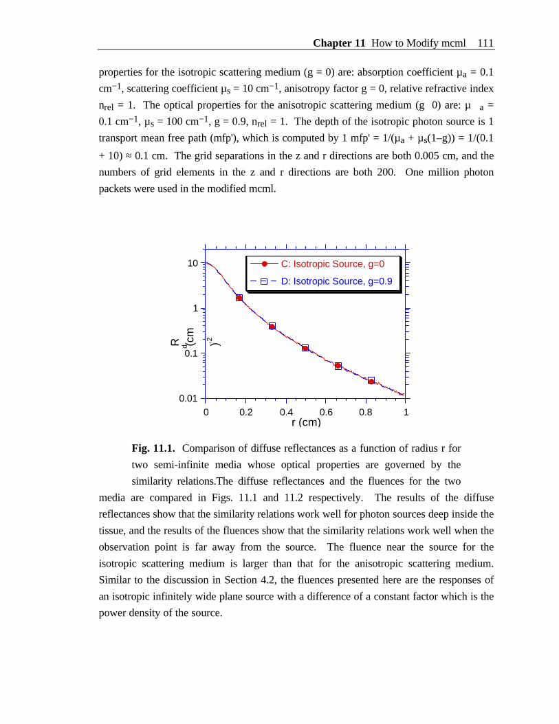
Chapter 11 How to Modify mcml 111
properties for the isotropic scattering medium (g = 0) are: absorption coefficient µa = 0.1
cm−1, scattering coefficient µs = 10 cm−1, anisotropy factor g = 0, relative refractive index
nrel = 1. The optical properties for the anisotropic scattering medium (g 0) are: µ a =
0.1 cm−1, µs = 100 cm−1, g = 0.9, nrel = 1. The depth of the isotropic photon source is 1
transport mean free path (mfp'), which is computed by 1 mfp' = 1/(µa + µs(1–g)) = 1/(0.1
+ 10) ≈ 0.1 cm. The grid separations in the z and r directions are both 0.005 cm, and the
numbers of grid elements in the z and r directions are both 200. One million photon
packets were used in the modified mcml.
0.01
0.1
1
10
0
R d (cm
-2 )
0.2 0.4 0.6 0.8 1r (cm)
C: Isotropic Source, g=0
D: Isotropic Source, g=0.9
Fig. 11.1. Comparison of diffuse reflectances as a function of radius r for
two semi-infinite media whose optical properties are governed by the
similarity relations.The diffuse reflectances and the fluences for the two
media are compared in Figs. 11.1 and 11.2 respectively. The results of the diffuse
reflectances show that the similarity relations work well for photon sources deep inside the
tissue, and the results of the fluences show that the similarity relations work well when the
observation point is far away from the source. The fluence near the source for the
isotropic scattering medium is larger than that for the anisotropic scattering medium.
Similar to the discussion in Section 4.2, the fluences presented here are the responses of
an isotropic infinitely wide plane source with a difference of a constant factor which is the
power density of the source.
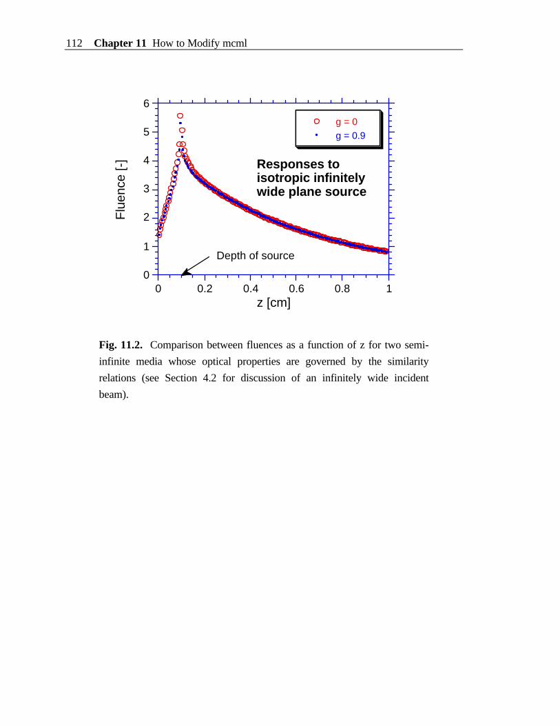
112 Chapter 11 How to Modify mcml
0
1
2
3
4
5
6
Flu
ence
[-]
0 0.2 0.4 0.6 0.8 1z [cm]
g = 0g = 0.9
Responses to isotropic infinitely wide plane source
Depth of source
Fig. 11.2. Comparison between fluences as a function of z for two semi-
infinite media whose optical properties are governed by the similarity
relations (see Section 4.2 for discussion of an infinitely wide incident
beam).

Appendix A Cflow Output of the Program mcml 113
Appendices
Appendix A. Cflow Output of the Program mcml
We have listed the short format of the UNIX command cflow output in Section
5.5. To show all depth of the nesting levels, we list here the results of the UNIX
command:
cflow mcmlgo.c
1 main: char(), <mcmlmain.c 198>2 ShowVersion: void*(), <mcmlio.c 49>3 CenterStr: char*(), <mcmlio.c 28>4 strlen: <>5 strcpy: <>6 strcat: <>7 puts: <>8 GetFnameFromArgv: void*(), <mcmlmain.c 150>9 strcpy: 510 GetFile: struct*(), <mcmlio.c 94>11 printf: <>12 scanf: <>13 strlen: 414 exit: <>15 fopen: <>16 CheckParm: void*(), <mcmlio.c 514>17 ReadNumRuns: short(), <mcmlio.c 205>18 FindDataLine: char*(), <mcmlio.c 184>19 fgets: <>20 printf: 1121 CheckChar: char(), <mcmlio.c 139>22 strlen: 423 nrerror: void*(), <mcmlnr.c 19>24 fprintf: <>25 exit: 1426 KillChar: void*(), <mcmlio.c 123>27 CommentLine: char(), <mcmlio.c 165>28 strspn: <>29 strcspn: <>30 strcpy: 531 nrerror: 2332 sscanf: <>33 printf: 1134 ReadParm: void*(), <mcmlio.c 425>35 ReadFnameFormat: void*(), <mcmlio.c 225>36 FindDataLine: 1837 strcpy: 538 nrerror: 2339 sscanf: 3240 toupper: <>41 ReadNumPhotons: void*(), <mcmlio.c 243>42 FindDataLine: 1843 strcpy: 544 nrerror: 2345 sscanf: 3246 ReadDzDr: void*(), <mcmlio.c 260>47 FindDataLine: 1848 strcpy: 549 nrerror: 2350 sscanf: 32
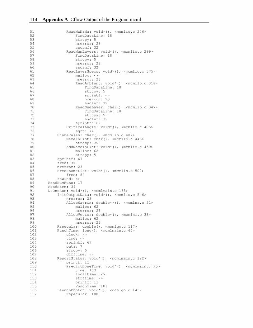
114 Appendix A Cflow Output of the Program mcml
51 ReadNzNrNa: void*(), <mcmlio.c 276>52 FindDataLine: 1853 strcpy: 554 nrerror: 2355 sscanf: 3256 ReadNumLayers: void*(), <mcmlio.c 299>57 FindDataLine: 1858 strcpy: 559 nrerror: 2360 sscanf: 3261 ReadLayerSpecs: void*(), <mcmlio.c 375>62 malloc: <>63 nrerror: 2364 ReadAmbient: void*(), <mcmlio.c 318>65 FindDataLine: 1866 strcpy: 567 sprintf: <>68 nrerror: 2369 sscanf: 3270 ReadOneLayer: char(), <mcmlio.c 347>71 FindDataLine: 1872 strcpy: 573 sscanf: 3274 sprintf: 6775 CriticalAngle: void*(), <mcmlio.c 405>76 sqrt: <>77 FnameTaken: char(), <mcmlio.c 487>78 NameInList: char(), <mcmlio.c 446>79 strcmp: <>80 AddNameToList: void*(), <mcmlio.c 459>81 malloc: 6282 strcpy: 583 sprintf: 6784 free: <>85 nrerror: 2386 FreeFnameList: void*(), <mcmlio.c 500>87 free: 8488 rewind: <>89 ReadNumRuns: 1790 ReadParm: 3491 DoOneRun: void*(), <mcmlmain.c 163>92 InitOutputData: void*(), <mcmlio.c 546>93 nrerror: 2394 AllocMatrix: double**(), <mcmlnr.c 52>95 malloc: 6296 nrerror: 2397 AllocVector: double*(), <mcmlnr.c 33>98 malloc: 6299 nrerror: 23100 Rspecular: double(), <mcmlgo.c 117>101 PunchTime: long(), <mcmlmain.c 60>102 clock: <>103 time: <>104 sprintf: 67105 puts: 7106 strcpy: 5107 difftime: <>108 ReportStatus: void*(), <mcmlmain.c 122>109 printf: 11110 PredictDoneTime: void*(), <mcmlmain.c 95>111 time: 103112 localtime: <>113 strftime: <>114 printf: 11115 PunchTime: 101116 LaunchPhoton: void*(), <mcmlgo.c 143>117 Rspecular: 100
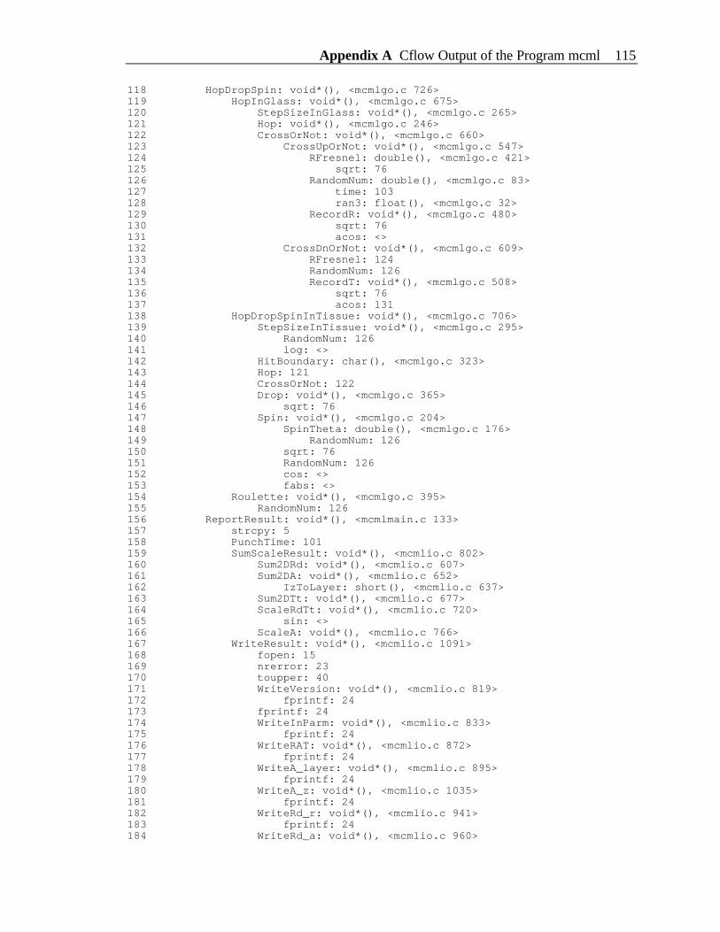
Appendix A Cflow Output of the Program mcml 115
118 HopDropSpin: void*(), <mcmlgo.c 726>119 HopInGlass: void*(), <mcmlgo.c 675>120 StepSizeInGlass: void*(), <mcmlgo.c 265>121 Hop: void*(), <mcmlgo.c 246>122 CrossOrNot: void*(), <mcmlgo.c 660>123 CrossUpOrNot: void*(), <mcmlgo.c 547>124 RFresnel: double(), <mcmlgo.c 421>125 sqrt: 76126 RandomNum: double(), <mcmlgo.c 83>127 time: 103128 ran3: float(), <mcmlgo.c 32>129 RecordR: void*(), <mcmlgo.c 480>130 sqrt: 76131 acos: <>132 CrossDnOrNot: void*(), <mcmlgo.c 609>133 RFresnel: 124134 RandomNum: 126135 RecordT: void*(), <mcmlgo.c 508>136 sqrt: 76137 acos: 131138 HopDropSpinInTissue: void*(), <mcmlgo.c 706>139 StepSizeInTissue: void*(), <mcmlgo.c 295>140 RandomNum: 126141 log: <>142 HitBoundary: char(), <mcmlgo.c 323>143 Hop: 121144 CrossOrNot: 122145 Drop: void*(), <mcmlgo.c 365>146 sqrt: 76147 Spin: void*(), <mcmlgo.c 204>148 SpinTheta: double(), <mcmlgo.c 176>149 RandomNum: 126150 sqrt: 76151 RandomNum: 126152 cos: <>153 fabs: <>154 Roulette: void*(), <mcmlgo.c 395>155 RandomNum: 126156 ReportResult: void*(), <mcmlmain.c 133>157 strcpy: 5158 PunchTime: 101159 SumScaleResult: void*(), <mcmlio.c 802>160 Sum2DRd: void*(), <mcmlio.c 607>161 Sum2DA: void*(), <mcmlio.c 652>162 IzToLayer: short(), <mcmlio.c 637>163 Sum2DTt: void*(), <mcmlio.c 677>164 ScaleRdTt: void*(), <mcmlio.c 720>165 sin: <>166 ScaleA: void*(), <mcmlio.c 766>167 WriteResult: void*(), <mcmlio.c 1091>168 fopen: 15169 nrerror: 23170 toupper: 40171 WriteVersion: void*(), <mcmlio.c 819>172 fprintf: 24173 fprintf: 24174 WriteInParm: void*(), <mcmlio.c 833>175 fprintf: 24176 WriteRAT: void*(), <mcmlio.c 872>177 fprintf: 24178 WriteA_layer: void*(), <mcmlio.c 895>179 fprintf: 24180 WriteA_z: void*(), <mcmlio.c 1035>181 fprintf: 24182 WriteRd_r: void*(), <mcmlio.c 941>183 fprintf: 24184 WriteRd_a: void*(), <mcmlio.c 960>
116 Appendix A Cflow Output of the Program mcml
185 fprintf: 24186 WriteTt_r: void*(), <mcmlio.c 1054>187 fprintf: 24188 WriteTt_a: void*(), <mcmlio.c 1073>189 fprintf: 24190 WriteA_rz: void*(), <mcmlio.c 1008>191 fprintf: 24192 WriteRd_ra: void*(), <mcmlio.c 914>193 fprintf: 24194 WriteTt_ra: void*(), <mcmlio.c 980>195 fprintf: 24196 fclose: <>197 FreeData: void*(), <mcmlio.c 581>198 free: 84199 FreeMatrix: void*(), <mcmlnr.c 86>200 free: 84201 FreeVector: void*(), <mcmlnr.c 77>202 free: 84203 fclose: 196
Section B.1 mcml.h 117
Appendix B. Source Code of the Program mcml
The whole program is divided into several files. The file "mcml.h" is the header
file, which defines data structures and some constants. The file "mcmlmain.c" contains the
function main(). It also deals with the timings and status report. The file "mcmlio.c"
reads or writes data from or to data files. The file "mcmlgo.c" does most of the Monte
Carlo simulations. The file "mcmlnr.c" (nr stands for numerical recipes) contains several
functions for dynamical data allocations and error report.
B.1 mcml.h
1 /*********************************************************** 2 * Copyright Univ. of Texas M.D. Anderson Cancer Center 3 * 1992. 4 * 5 * Monte Carlo simulation of photon distribution in 6 * multi-layered turbid media in ANSI Standard C. 7 **** 8 * Starting Date: 10/1991. 9 * Current Date: 6/1992. 10 * 11 * Lihong Wang, Ph. D. 12 * Steven L. Jacques, Ph. D. 13 * Laser Biology Research Laboratory - 17 14 * M.D. Anderson Cancer Center 15 * University of Texas 16 * 1515 Holcombe Blvd. 17 * Houston, TX 77030 18 * USA 19 * 20 * This program was based on: 21 * (1) The Pascal code written by Marleen Keijzer and 22 * Steven L. Jacques in this laboratory in 1989, which 23 * deals with multi-layered turbid media. 24 * 25 * (2) Algorithm for semi-infinite turbid medium by 26 * S.A. Prahl, M. Keijzer, S.L. Jacques, A.J. Welch, 27 * SPIE Institute Series Vol. IS 5 (1989), and by 28 * A.N. Witt, The Astrophysical journal Supplement 29 * Series 35, 1-6 (1977). 30 * 31 * Major modifications include: 32 * . Conform to ANSI Standard C. 33 * . Removal of limit on number of array elements, 34 * because arrays in this program are dynamically 35 * allocated. This means that the program can accept 36 * any number of layers or gridlines as long as the 37 * memory permits. 38 * . Avoiding global variables whenever possible. This 39 * program has not used global variables so far. 40 * . Grouping variables logically using structures. 41 * . Top-down design, keep each subroutine clear & 42 * short. 43 * . Reflectance and transmittance are angularly 44 * resolved. 45 **** 46 * General Naming Conventions:
118 Appendix B Source Code of the Program mcml
47 * Preprocessor names: all capital letters, 48 * e.g. #define PREPROCESSORS 49 * Globals: first letter of each word is capital, no 50 * underscores, 51 * e.g. short GlobalVar; 52 * Dummy variables: first letter of each word is capital, 53 * and words are connected by underscores, 54 * e.g. void NiceFunction(char Dummy_Var); 55 * Local variables: all lower cases, words are connected 56 * by underscores, 57 * e.g. short local_var; 58 * Function names or data types: same as Globals. 59 * 60 **** 61 * Dimension of length: cm. 62 * 63 ****/ 64 65 #include <math.h> 66 #include <stdlib.h> 67 #include <stdio.h> 68 #include <stddef.h> 69 #include <time.h> 70 #include <string.h> 71 #include <ctype.h> 72 73 #define PI 3.1415926 74 #define WEIGHT 1E-4 /* Critical weight for roulette. */ 75 #define CHANCE 0.1 /* Chance of roulette survival. */ 76 #define STRLEN 256 /* String length. */ 77 78 #define Boolean char 79 80 #define SIGN(x) ((x)>=0 ? 1:-1) 81 82 /****************** Stuctures *****************************/ 83 84 /**** 85 * Structure used to describe a photon packet. 86 ****/ 87 typedef struct 88 double x, y ,z; /* Cartesian coordinates.[cm] */ 89 double ux, uy, uz;/* directional cosines of a photon. */ 90 double w; /* weight. */ 91 Boolean dead; /* 1 if photon is terminated. */ 92 short layer; /* index to layer where the photon */ 93 /* packet resides. */ 94 double s; /* current step size. [cm]. */ 95 double sleft; /* step size left. dimensionless [-]. */ 96 PhotonStruct; 97 98 /**** 99 * Structure used to describe the geometry and optical 100 * properties of a layer. 101 * z0 and z1 are the z coordinates for the upper boundary 102 * and lower boundary respectively. 103 * 104 * cos_crit0 and cos_crit1 are the cosines of the 105 * critical angle of total internal reflection for the 106 * upper boundary and lower boundary respectively. 107 * They are set to zero if no total internal reflection 108 * exists. 109 * They are used for computation speed. 110 ****/ 111 typedef struct 112 double z0, z1; /* z coordinates of a layer. [cm] */ 113 double n; /* refractive index of a layer. */
Section B.1 mcml.h 119
114 double mua; /* absorption coefficient. [1/cm] */ 115 double mus; /* scattering coefficient. [1/cm] */ 116 double g; /* anisotropy. */ 117 118 double cos_crit0, cos_crit1; 119 LayerStruct; 120 121 /**** 122 * Input parameters for each independent run. 123 * 124 * z and r are for the cylindrical coordinate system. [cm] 125 * a is for the angle alpha between the photon exiting 126 * direction and the surface normal. [radian] 127 * 128 * The grid line separations in z, r, and alpha 129 * directions are dz, dr, and da respectively. The numbers 130 * of grid lines in z, r, and alpha directions are 131 * nz, nr, and na respectively. 132 * 133 * The member layerspecs will point to an array of 134 * structures which store parameters of each layer. 135 * This array has (number_layers + 2) elements. One 136 * element is for a layer. 137 * The layers 0 and (num_layers + 1) are for top ambient 138 * medium and the bottom ambient medium respectively. 139 ****/ 140 typedef struct 141 char out_fname[STRLEN]; /* output file name. */ 142 char out_fformat; /* output file format. */ 143 /* 'A' for ASCII, */ 144 /* 'B' for binary. */ 145 long num_photons; /* to be traced. */ 146 double Wth; /* play roulette if photon */ 147 /* weight < Wth.*/ 148 149 double dz; /* z grid separation.[cm] */ 150 double dr; /* r grid separation.[cm] */ 151 double da; /* alpha grid separation. */ 152 /* [radian] */ 153 short nz; /* array range 0..nz-1. */ 154 short nr; /* array range 0..nr-1. */ 155 short na; /* array range 0..na-1. */ 156 157 short num_layers; /* number of layers. */ 158 LayerStruct * layerspecs; /* layer parameters. */ 159 InputStruct; 160 161 /**** 162 * Structures for scoring physical quantities. 163 * z and r represent z and r coordinates of the 164 * cylindrical coordinate system. [cm] 165 * a is the angle alpha between the photon exiting 166 * direction and the normal to the surfaces. [radian] 167 * See comments of the InputStruct. 168 * See manual for the physcial quantities. 169 ****/ 170 typedef struct 171 double Rsp; /* specular reflectance. [-] */ 172 double ** Rd_ra; /* 2D distribution of diffuse */ 173 /* reflectance. [1/(cm2 sr)] */ 174 double * Rd_r; /* 1D radial distribution of diffuse */ 175 /* reflectance. [1/cm2] */ 176 double * Rd_a; /* 1D angular distribution of diffuse */ 177 /* reflectance. [1/sr] */ 178 double Rd; /* total diffuse reflectance. [-] */ 179 180 double ** A_rz; /* 2D probability density in turbid */
120 Appendix B Source Code of the Program mcml
181 /* media over r & z. [1/cm3] */ 182 double * A_z; /* 1D probability density over z. */ 183 /* [1/cm] */ 184 double * A_l; /* each layer's absorption */ 185 /* probability. [-] */ 186 double A; /* total absorption probability. [-] */ 187 188 double ** Tt_ra; /* 2D distribution of total */ 189 /* transmittance. [1/(cm2 sr)] */ 190 double * Tt_r; /* 1D radial distribution of */ 191 /* transmittance. [1/cm2] */ 192 double * Tt_a; /* 1D angular distribution of */ 193 /* transmittance. [1/sr] */ 194 double Tt; /* total transmittance. [-] */ 195 OutStruct; 196 197 /*********************************************************** 198 * Routine prototypes for dynamic memory allocation and 199 * release of arrays and matrices. 200 * Modified from Numerical Recipes in C. 201 ****/ 202 double *AllocVector(short, short); 203 double **AllocMatrix(short, short,short, short); 204 void FreeVector(double *, short, short); 205 void FreeMatrix(double **, short, short, short, short); 206 void nrerror(char *);
Section B.2 mcmlmain.c 121
B.2 mcmlmain.c
1 /*********************************************************** 2 * Copyright Univ. of Texas M.D. Anderson Cancer Center 3 * 1992. 4 * 5 * main program for Monte Carlo simulation of photon 6 * distribution in multi-layered turbid media. 7 * 8 ****/ 9 10 /**** 11 * THINKCPROFILER is defined to generate profiler calls in 12 * Think C. If 1, remember to turn on "Generate profiler 13 * calls" in the options menu. 14 ****/ 15 #define THINKCPROFILER 0 16 17 /* GNU cc does not support difftime() and CLOCKS_PER_SEC.*/ 18 #define GNUCC 0 19 20 #if THINKCPROFILER 21 #include <profile.h> 22 #include <console.h> 23 #endif 24 25 #include "mcml.h" 26 27 /* Declare before they are used in main(). */ 28 FILE *GetFile(char *); 29 short ReadNumRuns(FILE* ); 30 void ReadParm(FILE* , InputStruct * ); 31 void CheckParm(FILE* , InputStruct * ); 32 void InitOutputData(InputStruct, OutStruct *); 33 void FreeData(InputStruct, OutStruct *); 34 double Rspecular(LayerStruct * ); 35 void LaunchPhoton(double, LayerStruct *, PhotonStruct *); 36 void HopDropSpin(InputStruct *,PhotonStruct *,OutStruct *); 37 void SumScaleResult(InputStruct, OutStruct *); 38 void WriteResult(InputStruct, OutStruct, char *); 39 40 41 /*********************************************************** 42 * If F = 0, reset the clock and return 0. 43 * 44 * If F = 1, pass the user time to Msg and print Msg on 45 * screen, return the real time since F=0. 46 * 47 * If F = 2, same as F=1 except no printing. 48 * 49 * Note that clock() and time() return user time and real 50 * time respectively. 51 * User time is whatever the system allocates to the 52 * running of the program; 53 * real time is wall-clock time. In a time-shared system, 54 * they need not be the same. 55 * 56 * clock() only hold 16 bit integer, which is about 32768 57 * clock ticks. 58 ****/ 59 time_t PunchTime(char F, char *Msg) 60 61 #if GNUCC 62 return(0);
122 Appendix B Source Code of the Program mcml
63 #else 64 static clock_t ut0; /* user time reference. */ 65 static time_t rt0; /* real time reference. */ 66 double secs; 67 char s[STRLEN]; 68 69 if(F==0) 70 ut0 = clock(); 71 rt0 = time(NULL); 72 return(0); 73 74 else if(F==1) 75 secs = (clock() - ut0)/(double)CLOCKS_PER_SEC; 76 if (secs<0) secs=0; /* clock() can overflow. */ 77 sprintf(s, "User time: %8.0lf sec = %8.2lf hr. %s\n", 78 secs, secs/3600.0, Msg); 79 puts(s); 80 strcpy(Msg, s); 81 return(difftime(time(NULL), rt0)); 82 83 else if(F==2) return(difftime(time(NULL), rt0)); 84 else return(0); 85 #endif 86 87 88 /*********************************************************** 89 * Print the current time and the estimated finishing time. 90 * 91 * P1 is the number of computed photon packets. 92 * Pt is the total number of photon packets. 93 ****/ 94 void PredictDoneTime(long P1, long Pt) 95 96 time_t now, done_time; 97 struct tm *date; 98 char s[80]; 99 100 now = time(NULL); 101 date = localtime(&now); 102 strftime(s, 80, "%H:%M %x", date); 103 printf("Now %s, ", s); 104 105 done_time = now + 106 (time_t) (PunchTime(2,"")*(Pt-P1)/(double)P1); 107 date = localtime(&done_time); 108 strftime(s, 80, "%H:%M %x", date); 109 printf("End %s\n", s); 110 111 112 /*********************************************************** 113 * Report estimated time, number of photons and runs left 114 * after calculating 10 photons or every 1/10 of total 115 * number of photons. 116 * 117 * Num_Runs is the number of runs left. 118 * Pi is the index to the current photon, counting down. 119 * Pt is the total number of photons. 120 ****/ 121 void ReportStatus(short Num_Runs,long Pi,long Pt) 122 123 if(Pt-Pi == 10 || Pi*10%Pt == 0 && Pi != Pt) 124 printf("%ld photons & %hd runs left, ", Pi, Num_Runs); 125 PredictDoneTime(Pt-Pi, Pt); 126 127 128 129 /***********************************************************
Section B.2 mcmlmain.c 123
130 * Report time and write results. 131 ****/ 132 void ReportResult(InputStruct In_Parm, OutStruct Out_Parm) 133 134 char time_report[STRLEN]; 135 136 strcpy(time_report, " Simulation time of this run."); 137 PunchTime(1, time_report); 138 139 SumScaleResult(In_Parm, &Out_Parm); 140 WriteResult(In_Parm, Out_Parm, time_report); 141 142 143 /*********************************************************** 144 * Get the file name of the input data file from the 145 * argument to the command line. 146 ****/ 147 void GetFnameFromArgv(int argc, 148 char * argv[], 149 char * input_filename) 150 151 if(argc>=2) /* filename in command line */ 152 strcpy(input_filename, argv[1]); 153 154 else 155 input_filename[0] = '\0'; 156 157 158 159 /*********************************************************** 160 * Execute Monte Carlo simulation for one independent run. 161 ****/ 162 void DoOneRun(short NumRuns, InputStruct *In_Ptr) 163 164 register long i_photon; 165 /* index to photon. register for speed.*/ 166 OutStruct out_parm; /* distribution of photons.*/ 167 PhotonStruct photon; 168 169 #if THINKCPROFILER 170 InitProfile(200,200); cecho2file("prof.rpt",0, stdout); 171 #endif 172 173 InitOutputData(*In_Ptr, &out_parm); 174 out_parm.Rsp = Rspecular(In_Ptr->layerspecs); 175 i_photon = In_Ptr->num_photons; 176 PunchTime(0, ""); 177 178 do 179 ReportStatus(NumRuns, i_photon, In_Ptr->num_photons); 180 LaunchPhoton(out_parm.Rsp, In_Ptr->layerspecs, &photon); 181 do HopDropSpin(In_Ptr, &photon, &out_parm); 182 while (!photon.dead); 183 while(--i_photon); 184 185 #if THINKCPROFILER 186 exit(0); 187 #endif 188 189 ReportResult(*In_Ptr, out_parm); 190 FreeData(*In_Ptr, &out_parm); 191 192 193 /*********************************************************** 194 * The argument to the command line is filename, if any. 195 * Macintosh does not support command line. 196 ****/

124 Appendix B Source Code of the Program mcml
197 char main(int argc, char *argv[]) 198 199 char input_filename[STRLEN]; 200 FILE *input_file_ptr; 201 short num_runs; /* number of independent runs. */ 202 InputStruct in_parm; 203 204 ShowVersion("Version 1.1, 1992"); 205 GetFnameFromArgv(argc, argv, input_filename); 206 input_file_ptr = GetFile(input_filename); 207 CheckParm(input_file_ptr, &in_parm); 208 num_runs = ReadNumRuns(input_file_ptr); 209 210 while(num_runs--) 211 ReadParm(input_file_ptr, &in_parm); 212 DoOneRun(num_runs, &in_parm); 213 214 215 fclose(input_file_ptr); 216 return(0); 217
Section B.3 mcmlio.c 125
B.3 mcmlio.c
1 /*********************************************************** 2 * Copyright Univ. of Texas M.D. Anderson Cancer Center 3 * 1992. 4 * 5 * Input/output of data. 6 ****/ 7 8 #include "mcml.h" 9 10 /*********************************************************** 11 * Structure used to check against duplicated file names. 12 ****/ 13 struct NameList 14 char name[STRLEN]; 15 struct NameList * next; 16 ; 17 18 typedef struct NameList NameNode; 19 typedef NameNode * NameLink; 20 21 22 /*********************************************************** 23 * Center a string according to the column width. 24 ****/ 25 char * CenterStr(short Wid, 26 char * InStr, 27 char * OutStr) 28 29 size_t nspaces; /* number of spaces to be filled */ 30 /* before InStr. */ 31 32 nspaces = (Wid - strlen(InStr))/2; 33 if(nspaces<0) nspaces = 0; 34 35 strcpy(OutStr, ""); 36 while(nspaces--) strcat(OutStr, " "); 37 38 strcat(OutStr, InStr); 39 40 return(OutStr); 41 42 43 /*********************************************************** 44 * Print some messages before starting simulation. 45 * e.g. author, address, program version, year. 46 ****/ 47 #define COLWIDTH 80 48 void ShowVersion(char *version) 49 50 char str[STRLEN]; 51 52 CenterStr(COLWIDTH, 53 "mcml - Monte Carlo Simulation of Multi-layered Turbid Media", 54 str); 55 puts(str); 56 puts(""); 57 58 CenterStr(COLWIDTH, "Lihong Wang, Ph. D.", str); 59 puts(str); 60 61 CenterStr(COLWIDTH, "Steven L. Jacques, Ph. D.", str); 62 puts(str);
126 Appendix B Source Code of the Program mcml
63 64 CenterStr(COLWIDTH, 65 "Laser Biology Research Laboratory - Box 17",str); 66 puts(str); 67 68 CenterStr(COLWIDTH, "M.D. Anderson Cancer Center", str); 69 puts(str); 70 71 CenterStr(COLWIDTH, "University of Texas", str); 72 puts(str); 73 74 CenterStr(COLWIDTH, "Houston, TX 77030", str); 75 puts(str); 76 77 CenterStr(COLWIDTH, "Fax: (713)792-3995", str); 78 puts(str); 79 puts(""); 80 81 CenterStr(COLWIDTH, version, str); 82 puts(str); 83 puts("\n\n\n\n"); 84 85 #undef COLWIDTH 86 87 /*********************************************************** 88 * Get a filename and open it for reading, retry until 89 * the file can be opened. '.' terminates the program. 90 * 91 * If Fname != NULL, try Fname first. 92 ****/ 93 FILE *GetFile(char *Fname) 94 95 FILE * file=NULL; 96 Boolean firsttime=1; 97 98 do 99 if(firsttime && Fname[0]!='\0') 100 /* use the filename from command line */ 101 firsttime = 0; 102 103 else 104 printf("Input filename(or . to exit):"); 105 scanf("%s", Fname); 106 firsttime = 0; 107 108 109 if(strlen(Fname) == 1 && Fname[0] == '.') 110 exit(1); /* exit if no filename entered. */ 111 112 file = fopen(Fname, "r"); 113 while(file == NULL); 114 115 return(file); 116 117 118 /*********************************************************** 119 * Kill the ith char (counting from 0), push the following 120 * chars forward by one. 121 ****/ 122 void KillChar(size_t i, char * Str) 123 124 size_t sl = strlen(Str); 125 126 for(;i<sl;i++) Str[i] = Str[i+1]; 127 128 129 /***********************************************************
Section B.3 mcmlio.c 127
130 * Eliminate the chars in a string which are not printing 131 * chars or spaces. 132 * 133 * Spaces include ' ', '\f', '\t' etc. 134 * 135 * Return 1 if no nonprinting chars found, otherwise 136 * return 0. 137 ****/ 138 Boolean CheckChar(char * Str) 139 140 Boolean found = 0; /* found bad char. */ 141 size_t sl = strlen(Str); 142 size_t i=0; 143 144 while(i<sl) 145 if (Str[i]<0 || Str[i]>255) 146 nrerror("Non-ASCII file\n"); 147 else if(isprint(Str[i]) || isspace(Str[i])) 148 i++; 149 else 150 found = 1; 151 KillChar(i, Str); 152 sl--; 153 154 155 return(found); 156 157 158 /*********************************************************** 159 * Return 1 if this line is a comment line in which the 160 * first non-space character is "#". 161 * 162 * Also return 1 if this line is space line. 163 ****/ 164 Boolean CommentLine(char *Buf) 165 166 size_t spn, cspn; 167 168 spn = strspn(Buf, " \t"); 169 /* length spanned by space or tab chars. */ 170 171 cspn = strcspn(Buf, "#\n"); 172 /* length before the 1st # or return. */ 173 174 if(spn == cspn) /* comment line or space line. */ 175 return(1); 176 else /* the line has data. */ 177 return(0); 178 179 180 /*********************************************************** 181 * Skip space or comment lines and return a data line only. 182 ****/ 183 char * FindDataLine(FILE *File_Ptr) 184 185 char buf[STRLEN]; 186 187 buf[0] = '\0'; 188 do /* skip space or comment lines. */ 189 if(fgets(buf, 255, File_Ptr) == NULL) 190 printf("Incomplete data\n"); 191 buf[0]='\0'; 192 break; 193 194 else 195 CheckChar(buf); 196 while(CommentLine(buf));
128 Appendix B Source Code of the Program mcml
197 198 return(buf); 199 200 201 /*********************************************************** 202 * Skip file version, then read number of runs. 203 ****/ 204 short ReadNumRuns(FILE* File_Ptr) 205 206 char buf[STRLEN]; 207 short n=0; 208 209 FindDataLine(File_Ptr); /* skip file version. */ 210 211 strcpy(buf, FindDataLine(File_Ptr)); 212 if(buf[0]=='\0') nrerror("Reading number of runs\n"); 213 sscanf(buf, "%hd",&n); 214 return(n); 215 216 217 218 /*********************************************************** 219 * Read the file name and the file format. 220 * 221 * The file format can be either A for ASCII or B for 222 * binary. 223 ****/ 224 void ReadFnameFormat(FILE *File_Ptr, InputStruct *In_Ptr) 225 226 char buf[STRLEN]; 227 228 /** read in file name and format. **/ 229 strcpy(buf, FindDataLine(File_Ptr)); 230 if(buf[0]=='\0') 231 nrerror("Reading file name and format.\n"); 232 sscanf(buf, "%s %c", 233 In_Ptr->out_fname, &(In_Ptr->out_fformat) ); 234 if(toupper(In_Ptr->out_fformat) != 'B') 235 In_Ptr->out_fformat = 'A'; 236 237 238 239 /*********************************************************** 240 * Read the number of photons. 241 ****/ 242 void ReadNumPhotons(FILE *File_Ptr, InputStruct *In_Ptr) 243 244 char buf[STRLEN]; 245 246 /** read in number of photons. **/ 247 strcpy(buf, FindDataLine(File_Ptr)); 248 if(buf[0]=='\0') 249 nrerror("Reading number of photons.\n"); 250 sscanf(buf, "%ld", &In_Ptr->num_photons); 251 if(In_Ptr->num_photons<=0) 252 nrerror("Nonpositive number of photons.\n"); 253 254 255 256 /*********************************************************** 257 * Read the members dz and dr. 258 ****/ 259 void ReadDzDr(FILE *File_Ptr, InputStruct *In_Ptr) 260 261 char buf[STRLEN]; 262 263 /** read in dz, dr. **/
Section B.3 mcmlio.c 129
264 strcpy(buf, FindDataLine(File_Ptr)); 265 if(buf[0]=='\0') nrerror("Reading dz, dr.\n"); 266 sscanf(buf, "%lf%lf", &In_Ptr->dz, &In_Ptr->dr); 267 if(In_Ptr->dz<=0) nrerror("Nonpositive dz.\n"); 268 if(In_Ptr->dr<=0) nrerror("Nonpositive dr.\n"); 269 270 271 272 /*********************************************************** 273 * Read the members nz, nr, na. 274 ****/ 275 void ReadNzNrNa(FILE *File_Ptr, InputStruct *In_Ptr) 276 277 char buf[STRLEN]; 278 279 /** read in number of dz, dr, da. **/ 280 strcpy(buf, FindDataLine(File_Ptr)); 281 if(buf[0]=='\0') 282 nrerror("Reading number of dz, dr, da's.\n"); 283 sscanf(buf, "%hd%hd%hd", 284 &In_Ptr->nz, &In_Ptr->nr, &In_Ptr->na); 285 if(In_Ptr->nz<=0) 286 nrerror("Nonpositive number of dz's.\n"); 287 if(In_Ptr->nr<=0) 288 nrerror("Nonpositive number of dr's.\n"); 289 if(In_Ptr->na<=0) 290 nrerror("Nonpositive number of da's.\n"); 291 In_Ptr->da = 0.5*PI/In_Ptr->na; 292 293 294 295 /*********************************************************** 296 * Read the number of layers. 297 ****/ 298 void ReadNumLayers(FILE *File_Ptr, InputStruct *In_Ptr) 299 300 char buf[STRLEN]; 301 302 /** read in number of layers. **/ 303 strcpy(buf, FindDataLine(File_Ptr)); 304 if(buf[0]=='\0') 305 nrerror("Reading number of layers.\n"); 306 sscanf(buf, "%hd", &In_Ptr->num_layers); 307 if(In_Ptr->num_layers<=0) 308 nrerror("Nonpositive number of layers.\n"); 309 310 311 312 /*********************************************************** 313 * Read the refractive index n of the ambient. 314 ****/ 315 void ReadAmbient(FILE *File_Ptr, 316 LayerStruct * Layer_Ptr, 317 char *side) 318 319 char buf[STRLEN], msg[STRLEN]; 320 double n; 321 322 strcpy(buf, FindDataLine(File_Ptr)); 323 if(buf[0]=='\0') 324 sprintf(msg, "Rading n of %s ambient.\n", side); 325 nrerror(msg); 326 327 328 sscanf(buf, "%lf", &n ); 329 if(n<=0) nrerror("Wrong n.\n"); 330 Layer_Ptr->n = n;
130 Appendix B Source Code of the Program mcml
331 332 333 334 /*********************************************************** 335 * Read the parameters of one layer. 336 * 337 * Return 1 if error detected. 338 * Return 0 otherwise. 339 * 340 * *Z_Ptr is the z coordinate of the current layer, which 341 * is used to convert thickness of layer to z coordinates 342 * of the two boundaries of the layer. 343 ****/ 344 Boolean ReadOneLayer(FILE *File_Ptr, 345 LayerStruct * Layer_Ptr, 346 double *Z_Ptr) 347 348 char buf[STRLEN], msg[STRLEN]; 349 double d, n, mua, mus, g; /* d is thickness. */ 350 351 strcpy(buf, FindDataLine(File_Ptr)); 352 if(buf[0]=='\0') return(1); /* error. */ 353 354 sscanf(buf, "%lf%lf%lf%lf%lf", &n, &mua, &mus, &g, &d); 355 if(d<0 || n<=0 || mua<0 || mus<0 || g<0 || g>1) 356 return(1); /* error. */ 357 358 Layer_Ptr->n = n; 359 Layer_Ptr->mua = mua; 360 Layer_Ptr->mus = mus; 361 Layer_Ptr->g = g; 362 Layer_Ptr->z0 = *Z_Ptr; 363 *Z_Ptr += d; 364 Layer_Ptr->z1 = *Z_Ptr; 365 366 return(0); 367 368 369 /*********************************************************** 370 * Read the parameters of one layer at a time. 371 ****/ 372 void ReadLayerSpecs(FILE *File_Ptr, 373 short Num_Layers, 374 LayerStruct ** Layerspecs_PP) 375 376 char msg[STRLEN]; 377 short i=0; 378 double z = 0.0; /* z coordinate of the current layer. */ 379 380 /* Allocate an array for the layer parameters. */ 381 /* layer 0 and layer Num_Layers + 1 are for ambient. */ 382 *Layerspecs_PP = (LayerStruct *) 383 malloc((unsigned) (Num_Layers+2)*sizeof(LayerStruct)); 384 if (!(*Layerspecs_PP)) 385 nrerror("allocation failure in ReadLayerSpecs()"); 386 387 ReadAmbient(File_Ptr, &((*Layerspecs_PP)[i]), "top"); 388 for(i=1; i<=Num_Layers; i++) 389 if(ReadOneLayer(File_Ptr, &((*Layerspecs_PP)[i]), &z)) 390 sprintf(msg, "Error reading %hd of %hd layers\n", 391 i, Num_Layers); 392 nrerror(msg); 393 394 ReadAmbient(File_Ptr, &((*Layerspecs_PP)[i]), "bottom"); 395 396 397 /***********************************************************
Section B.3 mcmlio.c 131
398 * Compute the critical angles for total internal 399 * reflection according to the relative refractive index 400 * of the layer. 401 * All layers are processed. 402 ****/ 403 void CriticalAngle( short Num_Layers, 404 LayerStruct ** Layerspecs_PP) 405 406 short i=0; 407 double n1, n2; 408 409 for(i=1; i<=Num_Layers; i++) 410 n1 = (*Layerspecs_PP)[i].n; 411 n2 = (*Layerspecs_PP)[i-1].n; 412 (*Layerspecs_PP)[i].cos_crit0 = n1>n2 ? 413 sqrt(1.0 - n2*n2/(n1*n1)) : 0.0; 414 415 n2 = (*Layerspecs_PP)[i+1].n; 416 (*Layerspecs_PP)[i].cos_crit1 = n1>n2 ? 417 sqrt(1.0 - n2*n2/(n1*n1)) : 0.0; 418 419 420 421 /*********************************************************** 422 * Read in the input parameters for one run. 423 ****/ 424 void ReadParm(FILE* File_Ptr, InputStruct * In_Ptr) 425 426 char buf[STRLEN]; 427 428 In_Ptr->Wth = WEIGHT; 429 430 ReadFnameFormat(File_Ptr, In_Ptr); 431 ReadNumPhotons(File_Ptr, In_Ptr); 432 ReadDzDr(File_Ptr, In_Ptr); 433 ReadNzNrNa(File_Ptr, In_Ptr); 434 ReadNumLayers(File_Ptr, In_Ptr); 435 436 ReadLayerSpecs(File_Ptr, In_Ptr->num_layers, 437 &In_Ptr->layerspecs); 438 CriticalAngle(In_Ptr->num_layers, &In_Ptr->layerspecs); 439 440 441 /*********************************************************** 442 * Return 1, if the name in the name list. 443 * Return 0, otherwise. 444 ****/ 445 Boolean NameInList(char *Name, NameLink List) 446 447 while (List != NULL) 448 if(strcmp(Name, List->name) == 0) 449 return(1); 450 List = List->next; 451 ; 452 return(0); 453 454 455 /*********************************************************** 456 * Add the name to the name list. 457 ****/ 458 void AddNameToList(char *Name, NameLink * List_Ptr) 459 460 NameLink list = *List_Ptr; 461 462 if(list == NULL) /* first node. */ 463 *List_Ptr = list = (NameLink)malloc(sizeof(NameNode)); 464 strcpy(list->name, Name);
132 Appendix B Source Code of the Program mcml
465 list->next = NULL; 466 467 else /* subsequent nodes. */ 468 /* Move to the last node. */ 469 while(list->next != NULL) 470 list = list->next; 471 472 /* Append a node to the list. */ 473 list->next = (NameLink)malloc(sizeof(NameNode)); 474 list = list->next; 475 strcpy(list->name, Name); 476 list->next = NULL; 477 478 479 480 /*********************************************************** 481 * Check against duplicated file names. 482 * 483 * A linked list is set up to store the file names used 484 * in this input data file. 485 ****/ 486 Boolean FnameTaken(char *fname, NameLink * List_Ptr) 487 488 if(NameInList(fname, *List_Ptr)) 489 return(1); 490 else 491 AddNameToList(fname, List_Ptr); 492 return(0); 493 494 495 496 /*********************************************************** 497 * Free each node in the file name list. 498 ****/ 499 void FreeFnameList(NameLink List) 500 501 NameLink next; 502 503 while(List != NULL) 504 next = List->next; 505 free(List); 506 List = next; 507 508 509 510 /*********************************************************** 511 * Check the input parameters for each run. 512 ****/ 513 void CheckParm(FILE* File_Ptr, InputStruct * In_Ptr) 514 515 short i_run; 516 short num_runs; /* number of independent runs. */ 517 NameLink head = NULL; 518 Boolean name_taken;/* output files share the same */ 519 /* file name.*/ 520 char msg[STRLEN]; 521 522 num_runs = ReadNumRuns(File_Ptr); 523 for(i_run=1; i_run<=num_runs; i_run++) 524 printf("Checking input data for run %hd\n", i_run); 525 ReadParm(File_Ptr, In_Ptr); 526 527 name_taken = FnameTaken(In_Ptr->out_fname, &head); 528 if(name_taken) 529 sprintf(msg, "file name %s duplicated.\n", 530 In_Ptr->out_fname); 531
Section B.3 mcmlio.c 133
532 free(In_Ptr->layerspecs); 533 if(name_taken) nrerror(msg); 534 535 FreeFnameList(head); 536 rewind(File_Ptr); 537 538 539 540 /*********************************************************** 541 * Allocate the arrays in OutStruct for one run, and 542 * array elements are automatically initialized to zeros. 543 ****/ 544 void InitOutputData(InputStruct In_Parm, 545 OutStruct * Out_Ptr) 546 547 short nz = In_Parm.nz; 548 short nr = In_Parm.nr; 549 short na = In_Parm.na; 550 short nl = In_Parm.num_layers; 551 /* remember to use nl+2 because of 2 for ambient. */ 552 553 if(nz<=0 || nr<=0 || na<=0 || nl<=0) 554 nrerror("Wrong grid parameters.\n"); 555 556 /* Init pure numbers. */ 557 Out_Ptr->Rsp = 0.0; 558 Out_Ptr->Rd = 0.0; 559 Out_Ptr->A = 0.0; 560 Out_Ptr->Tt = 0.0; 561 562 /* Allocate the arrays and the matrices. */ 563 Out_Ptr->Rd_ra = AllocMatrix(0,nr-1,0,na-1); 564 Out_Ptr->Rd_r = AllocVector(0,nr-1); 565 Out_Ptr->Rd_a = AllocVector(0,na-1); 566 567 Out_Ptr->A_rz = AllocMatrix(0,nr-1,0,nz-1); 568 Out_Ptr->A_z = AllocVector(0,nz-1); 569 Out_Ptr->A_l = AllocVector(0,nl+1); 570 571 Out_Ptr->Tt_ra = AllocMatrix(0,nr-1,0,na-1); 572 Out_Ptr->Tt_r = AllocVector(0,nr-1); 573 Out_Ptr->Tt_a = AllocVector(0,na-1); 574 575 576 /*********************************************************** 577 * Undo what InitOutputData did. 578 * i.e. free the data allocations. 579 ****/ 580 void FreeData(InputStruct In_Parm, OutStruct * Out_Ptr) 581 582 short nz = In_Parm.nz; 583 short nr = In_Parm.nr; 584 short na = In_Parm.na; 585 short nl = In_Parm.num_layers; 586 /* remember to use nl+2 because of 2 for ambient. */ 587 588 free(In_Parm.layerspecs); 589 590 FreeMatrix(Out_Ptr->Rd_ra, 0,nr-1,0,na-1); 591 FreeVector(Out_Ptr->Rd_r, 0,nr-1); 592 FreeVector(Out_Ptr->Rd_a, 0,na-1); 593 594 FreeMatrix(Out_Ptr->A_rz, 0, nr-1, 0,nz-1); 595 FreeVector(Out_Ptr->A_z, 0, nz-1); 596 FreeVector(Out_Ptr->A_l, 0,nl+1); 597 598 FreeMatrix(Out_Ptr->Tt_ra, 0,nr-1,0,na-1);
134 Appendix B Source Code of the Program mcml
599 FreeVector(Out_Ptr->Tt_r, 0,nr-1); 600 FreeVector(Out_Ptr->Tt_a, 0,na-1); 601 602 603 /*********************************************************** 604 * Get 1D array elements by summing the 2D array elements. 605 ****/ 606 void Sum2DRd(InputStruct In_Parm, OutStruct * Out_Ptr) 607 608 short nr = In_Parm.nr; 609 short na = In_Parm.na; 610 short ir,ia; 611 double sum; 612 613 for(ir=0; ir<nr; ir++) 614 sum = 0.0; 615 for(ia=0; ia<na; ia++) sum += Out_Ptr->Rd_ra[ir][ia]; 616 Out_Ptr->Rd_r[ir] = sum; 617 618 619 for(ia=0; ia<na; ia++) 620 sum = 0.0; 621 for(ir=0; ir<nr; ir++) sum += Out_Ptr->Rd_ra[ir][ia]; 622 Out_Ptr->Rd_a[ia] = sum; 623 624 625 sum = 0.0; 626 for(ir=0; ir<nr; ir++) sum += Out_Ptr->Rd_r[ir]; 627 Out_Ptr->Rd = sum; 628 629 630 /*********************************************************** 631 * Return the index to the layer according to the index 632 * to the grid line system in z direction (Iz). 633 * 634 * Use the center of box. 635 ****/ 636 short IzToLayer(short Iz, InputStruct In_Parm) 637 638 short i=1; /* index to layer. */ 639 short num_layers = In_Parm.num_layers; 640 double dz = In_Parm.dz; 641 642 while( (Iz+0.5)*dz >= In_Parm.layerspecs[i].z1 643 && i<num_layers) i++; 644 645 return(i); 646 647 648 /*********************************************************** 649 * Get 1D array elements by summing the 2D array elements. 650 ****/ 651 void Sum2DA(InputStruct In_Parm, OutStruct * Out_Ptr) 652 653 short nz = In_Parm.nz; 654 short nr = In_Parm.nr; 655 short iz,ir; 656 double sum; 657 658 for(iz=0; iz<nz; iz++) 659 sum = 0.0; 660 for(ir=0; ir<nr; ir++) sum += Out_Ptr->A_rz[ir][iz]; 661 Out_Ptr->A_z[iz] = sum; 662 663 664 sum = 0.0; 665 for(iz=0; iz<nz; iz++)
Section B.3 mcmlio.c 135
666 sum += Out_Ptr->A_z[iz]; 667 Out_Ptr->A_l[IzToLayer(iz, In_Parm)] 668 += Out_Ptr->A_z[iz]; 669 670 Out_Ptr->A = sum; 671 672 673 /*********************************************************** 674 * Get 1D array elements by summing the 2D array elements. 675 ****/ 676 void Sum2DTt(InputStruct In_Parm, OutStruct * Out_Ptr) 677 678 short nr = In_Parm.nr; 679 short na = In_Parm.na; 680 short ir,ia; 681 double sum; 682 683 for(ir=0; ir<nr; ir++) 684 sum = 0.0; 685 for(ia=0; ia<na; ia++) sum += Out_Ptr->Tt_ra[ir][ia]; 686 Out_Ptr->Tt_r[ir] = sum; 687 688 689 for(ia=0; ia<na; ia++) 690 sum = 0.0; 691 for(ir=0; ir<nr; ir++) sum += Out_Ptr->Tt_ra[ir][ia]; 692 Out_Ptr->Tt_a[ia] = sum; 693 694 695 sum = 0.0; 696 for(ir=0; ir<nr; ir++) sum += Out_Ptr->Tt_r[ir]; 697 Out_Ptr->Tt = sum; 698 699 700 /*********************************************************** 701 * Scale Rd and Tt properly. 702 * 703 * "a" stands for angle alpha. 704 **** 705 * Scale Rd(r,a) and Tt(r,a) by 706 * (area perpendicular to photon direction) 707 * x(solid angle)x(No. of photons). 708 * or 709 * [2*PI*r*dr*cos(a)]x[2*PI*sin(a)*da]x[No. of photons] 710 * or 711 * [2*PI*PI*dr*da*r*sin(2a)]x[No. of photons] 712 **** 713 * Scale Rd(r) and Tt(r) by 714 * (area on the surface)x(No. of photons). 715 **** 716 * Scale Rd(a) and Tt(a) by 717 * (solid angle)x(No. of photons). 718 ****/ 719 void ScaleRdTt(InputStruct In_Parm, OutStruct * Out_Ptr) 720 721 short nr = In_Parm.nr; 722 short na = In_Parm.na; 723 double dr = In_Parm.dr; 724 double da = In_Parm.da; 725 short ir,ia; 726 double scale1, scale2; 727 728 scale1 = 4.0*PI*PI*dr*sin(da/2)*dr*In_Parm.num_photons; 729 /* The factor (ir+0.5)*sin(2a) to be added. */ 730 731 for(ir=0; ir<nr; ir++) 732 for(ia=0; ia<na; ia++)
136 Appendix B Source Code of the Program mcml
733 scale2 = 1.0/((ir+0.5)*sin(2.0*(ia+0.5)*da)*scale1); 734 Out_Ptr->Rd_ra[ir][ia] *= scale2; 735 Out_Ptr->Tt_ra[ir][ia] *= scale2; 736 737 738 scale1 = 2.0*PI*dr*dr*In_Parm.num_photons; 739 /* area is 2*PI*[(ir+0.5)*dr]*dr.*/ 740 /* ir+0.5 to be added. */ 741 742 for(ir=0; ir<nr; ir++) 743 scale2 = 1.0/((ir+0.5)*scale1); 744 Out_Ptr->Rd_r[ir] *= scale2; 745 Out_Ptr->Tt_r[ir] *= scale2; 746 747 748 scale1 = 2.0*PI*da*In_Parm.num_photons; 749 /* solid angle is 2*PI*sin(a)*da. sin(a) to be added. */ 750 751 for(ia=0; ia<na; ia++) 752 scale2 = 1.0/(sin((ia+0.5)*da)*scale1); 753 Out_Ptr->Rd_a[ia] *= scale2; 754 Out_Ptr->Tt_a[ia] *= scale2; 755 756 757 scale2 = 1.0/(double)In_Parm.num_photons; 758 Out_Ptr->Rd *= scale2; 759 Out_Ptr->Tt *= scale2; 760 761 762 /*********************************************************** 763 * Scale absorption arrays properly. 764 ****/ 765 void ScaleA(InputStruct In_Parm, OutStruct * Out_Ptr) 766 767 short nz = In_Parm.nz; 768 short nr = In_Parm.nr; 769 double dz = In_Parm.dz; 770 double dr = In_Parm.dr; 771 short nl = In_Parm.num_layers; 772 short iz,ir; 773 short il; 774 double scale1; 775 776 /* Scale A_rz. */ 777 scale1 = 2.0*PI*dr*dr*dz*In_Parm.num_photons; 778 /* volume is 2*pi*(ir+0.5)*dr*dr*dz.*/ 779 /* ir+0.5 to be added. */ 780 for(iz=0; iz<nz; iz++) 781 for(ir=0; ir<nr; ir++) 782 Out_Ptr->A_rz[ir][iz] /= (ir+0.5)*scale1; 783 784 /* Scale A_z. */ 785 scale1 = 1.0/(dz*In_Parm.num_photons); 786 for(iz=0; iz<nz; iz++) 787 Out_Ptr->A_z[iz] *= scale1; 788 789 /* Scale A_l. Avoid int/int. */ 790 scale1 = 1.0/(double)In_Parm.num_photons; 791 for(il=0; il<=nl+1; il++) 792 Out_Ptr->A_l[il] *= scale1; 793 794 Out_Ptr->A *=scale1; 795 796 797 /*********************************************************** 798 * Sum and scale results of current run. 799 ****/
Section B.3 mcmlio.c 137
800 void SumScaleResult(InputStruct In_Parm, 801 OutStruct * Out_Ptr) 802 803 /* Get 1D & 0D results. */ 804 Sum2DRd(In_Parm, Out_Ptr); 805 Sum2DA(In_Parm, Out_Ptr); 806 Sum2DTt(In_Parm, Out_Ptr); 807 808 ScaleRdTt(In_Parm, Out_Ptr); 809 ScaleA(In_Parm, Out_Ptr); 810 811 812 /*********************************************************** 813 * Write the version number as the first string in the 814 * file. 815 * Use chars only so that they can be read as either 816 * ASCII or binary. 817 ****/ 818 void WriteVersion(FILE *file, char *Version) 819 820 fprintf(file, 821 "%s \t# Version number of the file format.\n\n", 822 Version); 823 fprintf(file, "####\n# Data categories include: \n"); 824 fprintf(file, "# InParm, RAT, \n"); 825 fprintf(file, "# A_l, A_z, Rd_r, Rd_a, Tt_r, Tt_a, \n"); 826 fprintf(file, "# A_rz, Rd_ra, Tt_ra \n####\n\n"); 827 828 829 /*********************************************************** 830 * Write the input parameters to the file. 831 ****/ 832 void WriteInParm(FILE *file, InputStruct In_Parm) 833 834 short i; 835 836 fprintf(file, 837 "InParm \t\t\t# Input parameters. cm is used.\n"); 838 839 fprintf(file, 840 "%s \tA\t\t# output file name, ASCII.\n", 841 In_Parm.out_fname); 842 fprintf(file, 843 "%ld \t\t\t# No. of photons\n", In_Parm.num_photons); 844 845 fprintf(file, 846 "%G\t%G\t\t# dz, dr [cm]\n", In_Parm.dz,In_Parm.dr); 847 fprintf(file, "%hd\t%hd\t%hd\t# No. of dz, dr, da.\n\n", 848 In_Parm.nz, In_Parm.nr, In_Parm.na); 849 850 fprintf(file, 851 "%hd\t\t\t\t\t# Number of layers\n", 852 In_Parm.num_layers); 853 fprintf(file, 854 "#n\tmua\tmus\tg\td\t# One line for each layer\n"); 855 fprintf(file, 856 "%G\t\t\t\t\t# n for medium above\n", 857 In_Parm.layerspecs[0].n); 858 for(i=1; i<=In_Parm.num_layers; i++) 859 LayerStruct s; 860 s = In_Parm.layerspecs[i]; 861 fprintf(file, "%G\t%G\t%G\t%G\t%G\t# layer %hd\n", 862 s.n, s.mua, s.mus, s.g, s.z1-s.z0, i); 863 864 fprintf(file, "%G\t\t\t\t\t# n for medium below\n\n", 865 In_Parm.layerspecs[i].n); 866
138 Appendix B Source Code of the Program mcml
867 868 /*********************************************************** 869 * Write reflectance, absorption, transmission. 870 ****/ 871 void WriteRAT(FILE * file, OutStruct Out_Parm) 872 873 fprintf(file, 874 "RAT #Reflectance, absorption, transmission. \n"); 875 /* flag. */ 876 877 fprintf(file, 878 "%-14.6G \t#Specular reflectance [-]\n", Out_Parm.Rsp); 879 fprintf(file, 880 "%-14.6G \t#Diffuse reflectance [-]\n", Out_Parm.Rd); 881 fprintf(file, 882 "%-14.6G \t#Absorbed fraction [-]\n", Out_Parm.A); 883 fprintf(file, 884 "%-14.6G \t#Transmittance [-]\n", Out_Parm.Tt); 885 886 fprintf(file, "\n"); 887 888 889 /*********************************************************** 890 * Write absorption as a function of layer. 891 ****/ 892 void WriteA_layer(FILE * file, 893 short Num_Layers, 894 OutStruct Out_Parm) 895 896 short i; 897 898 fprintf(file, 899 "A_l #Absorption as a function of layer. [-]\n"); 900 /* flag. */ 901 902 for(i=1; i<=Num_Layers; i++) 903 fprintf(file, "%12.4G\n", Out_Parm.A_l[i]); 904 fprintf(file, "\n"); 905 906 907 /*********************************************************** 908 * 5 numbers each line. 909 ****/ 910 void WriteRd_ra(FILE * file, 911 short Nr, 912 short Na, 913 OutStruct Out_Parm) 914 915 short ir, ia; 916 917 fprintf(file, 918 "%s\n%s\n%s\n%s\n%s\n%s\n", /* flag. */ 919 "# Rd[r][angle]. [1/(cm2sr)].", 920 "# Rd[0][0], [0][1],..[0][na-1]", 921 "# Rd[1][0], [1][1],..[1][na-1]", 922 "# ...", 923 "# Rd[nr-1][0], [nr-1][1],..[nr-1][na-1]", 924 "Rd_ra"); 925 926 for(ir=0;ir<Nr;ir++) 927 for(ia=0;ia<Na;ia++) 928 fprintf(file, "%12.4E ", Out_Parm.Rd_ra[ir][ia]); 929 if( (ir*Na + ia + 1)%5 == 0) fprintf(file, "\n"); 930 931 932 fprintf(file, "\n"); 933
Section B.3 mcmlio.c 139
934 935 /*********************************************************** 936 * 1 number each line. 937 ****/ 938 void WriteRd_r(FILE * file, 939 short Nr, 940 OutStruct Out_Parm) 941 942 short ir; 943 944 fprintf(file, 945 "Rd_r #Rd[0], [1],..Rd[nr-1]. [1/cm2]\n"); /* flag. */ 946 947 for(ir=0;ir<Nr;ir++) 948 fprintf(file, "%12.4E\n", Out_Parm.Rd_r[ir]); 949 950 951 fprintf(file, "\n"); 952 953 954 /*********************************************************** 955 * 1 number each line. 956 ****/ 957 void WriteRd_a(FILE * file, 958 short Na, 959 OutStruct Out_Parm) 960 961 short ia; 962 963 fprintf(file, 964 "Rd_a #Rd[0], [1],..Rd[na-1]. [sr-1]\n"); /* flag. */ 965 966 for(ia=0;ia<Na;ia++) 967 fprintf(file, "%12.4E\n", Out_Parm.Rd_a[ia]); 968 969 970 fprintf(file, "\n"); 971 972 973 /*********************************************************** 974 * 5 numbers each line. 975 ****/ 976 void WriteTt_ra(FILE * file, 977 short Nr, 978 short Na, 979 OutStruct Out_Parm) 980 981 short ir, ia; 982 983 fprintf(file, 984 "%s\n%s\n%s\n%s\n%s\n%s\n", /* flag. */ 985 "# Tt[r][angle]. [1/(cm2sr)].", 986 "# Tt[0][0], [0][1],..[0][na-1]", 987 "# Tt[1][0], [1][1],..[1][na-1]", 988 "# ...", 989 "# Tt[nr-1][0], [nr-1][1],..[nr-1][na-1]", 990 "Tt_ra"); 991 992 for(ir=0;ir<Nr;ir++) 993 for(ia=0;ia<Na;ia++) 994 fprintf(file, "%12.4E ", Out_Parm.Tt_ra[ir][ia]); 995 if( (ir*Na + ia + 1)%5 == 0) fprintf(file, "\n"); 996 997 998 fprintf(file, "\n"); 999 1000
140 Appendix B Source Code of the Program mcml
1001 /***********************************************************1002 * 5 numbers each line.1003 ****/1004 void WriteA_rz(FILE * file,1005 short Nr,1006 short Nz,1007 OutStruct Out_Parm)1008 1009 short iz, ir;10101011 fprintf(file,1012 "%s\n%s\n%s\n%s\n%s\n%s\n", /* flag. */1013 "# A[r][z]. [1/cm3]",1014 "# A[0][0], [0][1],..[0][nz-1]",1015 "# A[1][0], [1][1],..[1][nz-1]",1016 "# ...",1017 "# A[nr-1][0], [nr-1][1],..[nr-1][nz-1]",1018 "A_rz");10191020 for(ir=0;ir<Nr;ir++)1021 for(iz=0;iz<Nz;iz++) 1022 fprintf(file, "%12.4E ", Out_Parm.A_rz[ir][iz]);1023 if( (ir*Nz + iz + 1)%5 == 0) fprintf(file, "\n");1024 10251026 fprintf(file, "\n");1027 10281029 /***********************************************************1030 * 1 number each line.1031 ****/1032 void WriteA_z(FILE * file,1033 short Nz,1034 OutStruct Out_Parm)1035 1036 short iz;10371038 fprintf(file,1039 "A_z #A[0], [1],..A[nz-1]. [1/cm]\n"); /* flag. */10401041 for(iz=0;iz<Nz;iz++) 1042 fprintf(file, "%12.4E\n", Out_Parm.A_z[iz]);1043 10441045 fprintf(file, "\n");1046 10471048 /***********************************************************1049 * 1 number each line.1050 ****/1051 void WriteTt_r(FILE * file,1052 short Nr,1053 OutStruct Out_Parm)1054 1055 short ir;10561057 fprintf(file,1058 "Tt_r #Tt[0], [1],..Tt[nr-1]. [1/cm2]\n"); /* flag. */10591060 for(ir=0;ir<Nr;ir++) 1061 fprintf(file, "%12.4E\n", Out_Parm.Tt_r[ir]);1062 10631064 fprintf(file, "\n");1065 10661067 /***********************************************************
Section B.3 mcmlio.c 141
1068 * 1 number each line.1069 ****/1070 void WriteTt_a(FILE * file,1071 short Na,1072 OutStruct Out_Parm)1073 1074 short ia;10751076 fprintf(file,1077 "Tt_a #Tt[0], [1],..Tt[na-1]. [sr-1]\n"); /* flag. */10781079 for(ia=0;ia<Na;ia++) 1080 fprintf(file, "%12.4E\n", Out_Parm.Tt_a[ia]);1081 10821083 fprintf(file, "\n");1084 10851086 /***********************************************************1087 ****/1088 void WriteResult(InputStruct In_Parm,1089 OutStruct Out_Parm,1090 char * TimeReport)1091 1092 FILE *file;10931094 file = fopen(In_Parm.out_fname, "w");1095 if(file == NULL) nrerror("Cannot open file to write.\n");10961097 if(toupper(In_Parm.out_fformat) == 'A')1098 WriteVersion(file, "A1");1099 else1100 WriteVersion(file, "B1");11011102 fprintf(file, "# %s", TimeReport);1103 fprintf(file, "\n");11041105 WriteInParm(file, In_Parm);1106 WriteRAT(file, Out_Parm);1107 /* reflectance, absorption, transmittance. */11081109 /* 1D arrays. */1110 WriteA_layer(file, In_Parm.num_layers, Out_Parm);1111 WriteA_z(file, In_Parm.nz, Out_Parm);1112 WriteRd_r(file, In_Parm.nr, Out_Parm);1113 WriteRd_a(file, In_Parm.na, Out_Parm);1114 WriteTt_r(file, In_Parm.nr, Out_Parm);1115 WriteTt_a(file, In_Parm.na, Out_Parm);11161117 /* 2D arrays. */1118 WriteA_rz(file, In_Parm.nr, In_Parm.nz, Out_Parm);1119 WriteRd_ra(file, In_Parm.nr, In_Parm.na, Out_Parm);1120 WriteTt_ra(file, In_Parm.nr, In_Parm.na, Out_Parm);11211122 fclose(file);1123
142 Appendix B Source Code of the Program mcml
B.4 mcmlgo.c
1 /*********************************************************** 2 * Copyright Univ. of Texas M.D. Anderson Cancer Center 3 * 1992. 4 * 5 * Launch, move, and record photon weight. 6 ****/ 7 8 #include "mcml.h" 9 10 #define STANDARDTEST 0 11 /* testing program using fixed rnd seed. */ 12 13 #define PARTIALREFLECTION 0 14 /* 1=split photon, 0=statistical reflection. */ 15 16 #define COSZERO (1.0-1.0E-12) 17 /* cosine of about 1e-6 rad. */ 18 19 #define COS90D 1.0E-6 20 /* cosine of about 1.57 - 1e-6 rad. */ 21 22 23 /*********************************************************** 24 * A random number generator from Numerical Recipes in C. 25 ****/ 26 #define MBIG 1000000000 27 #define MSEED 161803398 28 #define MZ 0 29 #define FAC 1.0E-9 30 31 float ran3(int *idum) 32 33 static int inext,inextp; 34 static long ma[56]; 35 static int iff=0; 36 long mj,mk; 37 int i,ii,k; 38 39 if (*idum < 0 || iff == 0) 40 iff=1; 41 mj=MSEED-(*idum < 0 ? -*idum : *idum); 42 mj %= MBIG; 43 ma[55]=mj; 44 mk=1; 45 for (i=1;i<=54;i++) 46 ii=(21*i) % 55; 47 ma[ii]=mk; 48 mk=mj-mk; 49 if (mk < MZ) mk += MBIG; 50 mj=ma[ii]; 51 52 for (k=1;k<=4;k++) 53 for (i=1;i<=55;i++) 54 ma[i] -= ma[1+(i+30) % 55]; 55 if (ma[i] < MZ) ma[i] += MBIG; 56 57 inext=0; 58 inextp=31; 59 *idum=1; 60 61 if (++inext == 56) inext=1; 62 if (++inextp == 56) inextp=1;
Section B.4 mcmlgo.c 143
63 mj=ma[inext]-ma[inextp]; 64 if (mj < MZ) mj += MBIG; 65 ma[inext]=mj; 66 return mj*FAC; 67 68 69 #undef MBIG 70 #undef MSEED 71 #undef MZ 72 #undef FAC 73 74 75 /*********************************************************** 76 * Generate a random number between 0 and 1. Take a 77 * number as seed the first time entering the function. 78 * The seed is limited to 1<<15. 79 * We found that when idum is too large, ran3 may return 80 * numbers beyond 0 and 1. 81 ****/ 82 double RandomNum(void) 83 84 static Boolean first_time=1; 85 static int idum; /* seed for ran3. */ 86 87 if(first_time) 88 #if STANDARDTEST /* Use fixed seed to test the program. */ 89 idum = - 1; 90 #else 91 idum = -(int)time(NULL)%(1<<15); 92 /* use 16-bit integer as the seed. */ 93 #endif 94 ran3(&idum); 95 first_time = 0; 96 idum = 1; 97 98 99 return( (double)ran3(&idum) ); 100 101 102 /*********************************************************** 103 * Compute the specular reflection. 104 * 105 * If the first layer is a turbid medium, use the Fresnel 106 * reflection from the boundary of the first layer as the 107 * specular reflectance. 108 * 109 * If the first layer is glass, multiple reflections in 110 * the first layer is considered to get the specular 111 * reflectance. 112 * 113 * The subroutine assumes the Layerspecs array is correctly 114 * initialized. 115 ****/ 116 double Rspecular(LayerStruct * Layerspecs_Ptr) 117 118 double r1, r2; 119 /* direct reflections from the 1st and 2nd layers. */ 120 double temp; 121 122 temp =(Layerspecs_Ptr[0].n - Layerspecs_Ptr[1].n) 123 /(Layerspecs_Ptr[0].n + Layerspecs_Ptr[1].n); 124 r1 = temp*temp; 125 126 if((Layerspecs_Ptr[1].mua == 0.0) 127 && (Layerspecs_Ptr[1].mus == 0.0)) /* glass layer. */ 128 temp = (Layerspecs_Ptr[1].n - Layerspecs_Ptr[2].n) 129 /(Layerspecs_Ptr[1].n + Layerspecs_Ptr[2].n);
144 Appendix B Source Code of the Program mcml
130 r2 = temp*temp; 131 r1 = r1 + (1-r1)*(1-r1)*r2/(1-r1*r2); 132 133 134 return (r1); 135 136 137 /*********************************************************** 138 * Initialize a photon packet. 139 ****/ 140 void LaunchPhoton(double Rspecular, 141 LayerStruct * Layerspecs_Ptr, 142 PhotonStruct * Photon_Ptr) 143 144 Photon_Ptr->w = 1.0 - Rspecular; 145 Photon_Ptr->dead = 0; 146 Photon_Ptr->layer = 1; 147 Photon_Ptr->s = 0; 148 Photon_Ptr->sleft= 0; 149 150 Photon_Ptr->x = 0.0; 151 Photon_Ptr->y = 0.0; 152 Photon_Ptr->z = 0.0; 153 Photon_Ptr->ux = 0.0; 154 Photon_Ptr->uy = 0.0; 155 Photon_Ptr->uz = 1.0; 156 157 if((Layerspecs_Ptr[1].mua == 0.0) 158 && (Layerspecs_Ptr[1].mus == 0.0)) /* glass layer. */ 159 Photon_Ptr->layer = 2; 160 Photon_Ptr->z = Layerspecs_Ptr[2].z0; 161 162 163 164 /*********************************************************** 165 * Choose (sample) a new theta angle for photon propagation 166 * according to the anisotropy. 167 * 168 * If anisotropy g is 0, then 169 * cos(theta) = 2*rand-1. 170 * otherwise 171 * sample according to the Henyey-Greenstein function. 172 * 173 * Returns the cosine of the polar deflection angle theta. 174 ****/ 175 double SpinTheta(double g) 176 177 double cost; 178 179 if(g == 0.0) 180 cost = 2*RandomNum() -1; 181 else 182 double temp = (1-g*g)/(1-g+2*g*RandomNum()); 183 cost = (1+g*g - temp*temp)/(2*g); 184 185 return(cost); 186 187 188 189 /*********************************************************** 190 * Choose a new direction for photon propagation by 191 * sampling the polar deflection angle theta and the 192 * azimuthal angle psi. 193 * 194 * Note: 195 * theta: 0 - pi so sin(theta) is always positive 196 * feel free to use sqrt() for cos(theta).
Section B.4 mcmlgo.c 145
197 * 198 * psi: 0 - 2pi 199 * for 0-pi sin(psi) is + 200 * for pi-2pi sin(psi) is - 201 ****/ 202 void Spin(double g, 203 PhotonStruct * Photon_Ptr) 204 205 double cost, sint; /* cosine and sine of the */ 206 /* polar deflection angle theta. */ 207 double cosp, sinp; /* cosine and sine of the */ 208 /* azimuthal angle psi. */ 209 double ux = Photon_Ptr->ux; 210 double uy = Photon_Ptr->uy; 211 double uz = Photon_Ptr->uz; 212 double psi; 213 214 cost = SpinTheta(g); 215 sint = sqrt(1.0 - cost*cost); 216 /* sqrt() is faster than sin(). */ 217 218 psi = 2.0*PI*RandomNum(); /* spin psi 0-2pi. */ 219 cosp = cos(psi); 220 if(psi<PI) 221 sinp = sqrt(1.0 - cosp*cosp); 222 /* sqrt() is faster than sin(). */ 223 else 224 sinp = - sqrt(1.0 - cosp*cosp); 225 226 if(fabs(uz) > COSZERO) /* normal incident. */ 227 Photon_Ptr->ux = sint*cosp; 228 Photon_Ptr->uy = sint*sinp; 229 Photon_Ptr->uz = cost*SIGN(uz); 230 /* SIGN() is faster than division. */ 231 232 else /* regular incident. */ 233 double temp = sqrt(1.0 - uz*uz); 234 Photon_Ptr->ux = sint*(ux*uz*cosp - uy*sinp) 235 /temp + ux*cost; 236 Photon_Ptr->uy = sint*(uy*uz*cosp + ux*sinp) 237 /temp + uy*cost; 238 Photon_Ptr->uz = -sint*cosp*temp + uz*cost; 239 240 241 242 /*********************************************************** 243 * Move the photon s away in the current layer of medium. 244 ****/ 245 void Hop(PhotonStruct * Photon_Ptr) 246 247 double s = Photon_Ptr->s; 248 249 Photon_Ptr->x += s*Photon_Ptr->ux; 250 Photon_Ptr->y += s*Photon_Ptr->uy; 251 Photon_Ptr->z += s*Photon_Ptr->uz; 252 253 254 /*********************************************************** 255 * If uz != 0, return the photon step size in glass, 256 * Otherwise, return 0. 257 * 258 * The step size is the distance between the current 259 * position and the boundary in the photon direction. 260 * 261 * Make sure uz !=0 before calling this function. 262 ****/ 263 void StepSizeInGlass(PhotonStruct * Photon_Ptr,
146 Appendix B Source Code of the Program mcml
264 InputStruct * In_Ptr) 265 266 double dl_b; /* step size to boundary. */ 267 short layer = Photon_Ptr->layer; 268 double uz = Photon_Ptr->uz; 269 270 /* Stepsize to the boundary. */ 271 if(uz>0.0) 272 dl_b = (In_Ptr->layerspecs[layer].z1 - Photon_Ptr->z) 273 /uz; 274 else if(uz<0.0) 275 dl_b = (In_Ptr->layerspecs[layer].z0 - Photon_Ptr->z) 276 /uz; 277 else 278 dl_b = 0.0; 279 280 Photon_Ptr->s = dl_b; 281 282 283 /*********************************************************** 284 * Pick a step size for a photon packet when it is in 285 * tissue. 286 * If the member sleft is zero, make a new step size 287 * with: -log(rnd)/(mua+mus). 288 * Otherwise, pick up the leftover in sleft. 289 * 290 * Layer is the index to layer. 291 * In_Ptr is the input parameters. 292 ****/ 293 void StepSizeInTissue(PhotonStruct * Photon_Ptr, 294 InputStruct * In_Ptr) 295 296 short layer = Photon_Ptr->layer; 297 double mua = In_Ptr->layerspecs[layer].mua; 298 double mus = In_Ptr->layerspecs[layer].mus; 299 300 if(Photon_Ptr->sleft == 0.0) /* make a new step. */ 301 double rnd; 302 303 do rnd = RandomNum(); 304 while( rnd <= 0.0 ); /* avoid zero. */ 305 Photon_Ptr->s = -log(rnd)/(mua+mus); 306 307 else /* take the leftover. */ 308 Photon_Ptr->s = Photon_Ptr->sleft/(mua+mus); 309 Photon_Ptr->sleft = 0.0; 310 311 312 313 /*********************************************************** 314 * Check if the step will hit the boundary. 315 * Return 1 if hit boundary. 316 * Return 0 otherwise. 317 * 318 * If the projected step hits the boundary, the members 319 * s and sleft of Photon_Ptr are updated. 320 ****/ 321 Boolean HitBoundary(PhotonStruct * Photon_Ptr, 322 InputStruct * In_Ptr) 323 324 double dl_b; /* length to boundary. */ 325 short layer = Photon_Ptr->layer; 326 double uz = Photon_Ptr->uz; 327 Boolean hit; 328 329 /* Distance to the boundary. */ 330 if(uz>0.0)
Section B.4 mcmlgo.c 147
331 dl_b = (In_Ptr->layerspecs[layer].z1 332 - Photon_Ptr->z)/uz; /* dl_b>0. */ 333 else if(uz<0.0) 334 dl_b = (In_Ptr->layerspecs[layer].z0 335 - Photon_Ptr->z)/uz; /* dl_b>0. */ 336 337 if(uz != 0.0 && Photon_Ptr->s > dl_b) 338 /* not horizontal & crossing. */ 339 double mut = In_Ptr->layerspecs[layer].mua 340 + In_Ptr->layerspecs[layer].mus; 341 342 Photon_Ptr->sleft = (Photon_Ptr->s - dl_b)*mut; 343 Photon_Ptr->s = dl_b; 344 hit = 1; 345 346 else 347 hit = 0; 348 349 return(hit); 350 351 352 /*********************************************************** 353 * Drop photon weight inside the tissue (not glass). 354 * 355 * The photon is assumed not dead. 356 * 357 * The weight drop is dw = w*mua/(mua+mus). 358 * 359 * The dropped weight is assigned to the absorption array 360 * elements. 361 ****/ 362 void Drop(InputStruct * In_Ptr, 363 PhotonStruct * Photon_Ptr, 364 OutStruct * Out_Ptr) 365 366 double dwa; /* absorbed weight.*/ 367 double x = Photon_Ptr->x; 368 double y = Photon_Ptr->y; 369 short iz, ir; /* index to z & r. */ 370 short layer = Photon_Ptr->layer; 371 double mua, mus; 372 373 /* compute array indices. */ 374 iz = (short)(Photon_Ptr->z/In_Ptr->dz); 375 if(iz>In_Ptr->nz-1) iz=In_Ptr->nz-1; 376 377 ir = (short)(sqrt(x*x+y*y)/In_Ptr->dr); 378 if(ir>In_Ptr->nr-1) ir=In_Ptr->nr-1; 379 380 /* update photon weight. */ 381 mua = In_Ptr->layerspecs[layer].mua; 382 mus = In_Ptr->layerspecs[layer].mus; 383 dwa = Photon_Ptr->w * mua/(mua+mus); 384 Photon_Ptr->w -= dwa; 385 386 /* assign dwa to the absorption array element. */ 387 Out_Ptr->A_rz[ir][iz] += dwa; 388 389 390 /*********************************************************** 391 * The photon weight is small, and the photon packet tries 392 * to survive a roulette. 393 ****/ 394 void Roulette(PhotonStruct * Photon_Ptr) 395 396 if(Photon_Ptr->w == 0.0) 397 Photon_Ptr->dead = 1;
148 Appendix B Source Code of the Program mcml
398 else if(RandomNum() < CHANCE) /* survived the roulette.*/ 399 Photon_Ptr->w /= CHANCE; 400 else 401 Photon_Ptr->dead = 1; 402 403 404 /*********************************************************** 405 * Compute the Fresnel reflectance. 406 * 407 * Make sure that the cosine of the incident angle a1 408 * is positive, and the case when the angle is greater 409 * than the critical angle is ruled out. 410 * 411 * Avoid trigonometric function operations as much as 412 * possible, because they are computation-intensive. 413 ****/ 414 double RFresnel(double n1, /* incident refractive index.*/ 415 double n2, /* transmit refractive index.*/ 416 double ca1, /* cosine of the incident */ 417 /* angle. 0<a1<90 degrees. */ 418 double * ca2_Ptr) /* pointer to the */ 419 /* cosine of the transmission */ 420 /* angle. a2>0. */ 421 422 double r; 423 424 if(n1==n2) /** matched boundary. **/ 425 *ca2_Ptr = ca1; 426 r = 0.0; 427 428 else if(ca1>COSZERO) /** normal incident. **/ 429 *ca2_Ptr = ca1; 430 r = (n2-n1)/(n2+n1); 431 r *= r; 432 433 else if(ca1<COS90D) /** very slant. **/ 434 *ca2_Ptr = 0.0; 435 r = 1.0; 436 437 else /** general. **/ 438 double sa1, sa2; 439 /* sine of the incident and transmission angles. */ 440 double ca2; 441 442 sa1 = sqrt(1-ca1*ca1); 443 sa2 = n1*sa1/n2; 444 if(sa2>=1.0) 445 /* double check for total internal reflection. */ 446 *ca2_Ptr = 0.0; 447 r = 1.0; 448 449 else 450 double cap, cam; /* cosines of the sum ap or */ 451 /* difference am of the two */ 452 /* angles. ap = a1+a2 */ 453 /* am = a1 - a2. */ 454 double sap, sam; /* sines. */ 455 456 *ca2_Ptr = ca2 = sqrt(1-sa2*sa2); 457 458 cap = ca1*ca2 - sa1*sa2; /* c+ = cc - ss. */ 459 cam = ca1*ca2 + sa1*sa2; /* c- = cc + ss. */ 460 sap = sa1*ca2 + ca1*sa2; /* s+ = sc + cs. */ 461 sam = sa1*ca2 - ca1*sa2; /* s- = sc - cs. */ 462 r = 0.5*sam*sam*(cam*cam+cap*cap)/(sap*sap*cam*cam); 463 /* rearranged for speed. */ 464
Section B.4 mcmlgo.c 149
465 466 return(r); 467 468 469 /*********************************************************** 470 * Record the photon weight exiting the first layer(uz<0), 471 * no matter whether the layer is glass or not, to the 472 * reflection array. 473 * 474 * Update the photon weight as well. 475 ****/ 476 void RecordR(double Refl, /* reflectance. */ 477 InputStruct * In_Ptr, 478 PhotonStruct * Photon_Ptr, 479 OutStruct * Out_Ptr) 480 481 double x = Photon_Ptr->x; 482 double y = Photon_Ptr->y; 483 short ir, ia; /* index to r & angle. */ 484 485 ir = (short)(sqrt(x*x+y*y)/In_Ptr->dr); 486 if(ir>In_Ptr->nr-1) ir=In_Ptr->nr-1; 487 488 ia = (short)(acos(-Photon_Ptr->uz)/In_Ptr->da); 489 if(ia>In_Ptr->na-1) ia=In_Ptr->na-1; 490 491 /* assign photon to the reflection array element. */ 492 Out_Ptr->Rd_ra[ir][ia] += Photon_Ptr->w*(1.0-Refl); 493 494 Photon_Ptr->w *= Refl; 495 496 497 /*********************************************************** 498 * Record the photon weight exiting the last layer(uz>0), 499 * no matter whether the layer is glass or not, to the 500 * transmittance array. 501 * 502 * Update the photon weight as well. 503 ****/ 504 void RecordT(double Refl, 505 InputStruct * In_Ptr, 506 PhotonStruct * Photon_Ptr, 507 OutStruct * Out_Ptr) 508 509 double x = Photon_Ptr->x; 510 double y = Photon_Ptr->y; 511 short ir, ia; /* index to r & angle. */ 512 513 ir = (short)(sqrt(x*x+y*y)/In_Ptr->dr); 514 if(ir>In_Ptr->nr-1) ir=In_Ptr->nr-1; 515 516 ia = (short)(acos(Photon_Ptr->uz)/In_Ptr->da); 517 if(ia>In_Ptr->na-1) ia=In_Ptr->na-1; 518 519 /* assign photon to the transmittance array element. */ 520 Out_Ptr->Tt_ra[ir][ia] += Photon_Ptr->w*(1.0-Refl); 521 522 Photon_Ptr->w *= Refl; 523 524 525 /*********************************************************** 526 * Decide whether the photon will be transmitted or 527 * reflected on the upper boundary (uz<0) of the current 528 * layer. 529 * 530 * If "layer" is the first layer, the photon packet will 531 * be partially transmitted and partially reflected if
150 Appendix B Source Code of the Program mcml
532 * PARTIALREFLECTION is set to 1, 533 * or the photon packet will be either transmitted or 534 * reflected determined statistically if PARTIALREFLECTION 535 * is set to 0. 536 * 537 * Record the transmitted photon weight as reflection. 538 * 539 * If the "layer" is not the first layer and the photon 540 * packet is transmitted, move the photon to "layer-1". 541 * 542 * Update the photon parmameters. 543 ****/ 544 void CrossUpOrNot(InputStruct * In_Ptr, 545 PhotonStruct * Photon_Ptr, 546 OutStruct * Out_Ptr) 547 548 double uz = Photon_Ptr->uz; /* z directional cosine. */ 549 double uz1; /* cosines of transmission alpha. always */ 550 /* positive. */ 551 double r=0.0; /* reflectance */ 552 short layer = Photon_Ptr->layer; 553 double ni = In_Ptr->layerspecs[layer].n; 554 double nt = In_Ptr->layerspecs[layer-1].n; 555 556 /* Get r. */ 557 if( - uz <= In_Ptr->layerspecs[layer].cos_crit0) 558 r=1.0; /* total internal reflection. */ 559 else r = RFresnel(ni, nt, -uz, &uz1); 560 561 #if PARTIALREFLECTION 562 if(layer == 1 && r<1.0) /* partially transmitted. */ 563 Photon_Ptr->uz = -uz1; /* transmitted photon. */ 564 RecordR(r, In_Ptr, Photon_Ptr, Out_Ptr); 565 Photon_Ptr->uz = -uz; /* reflected photon. */ 566 567 else if(RandomNum() > r) /* transmitted to layer-1. */ 568 Photon_Ptr->layer--; 569 Photon_Ptr->ux *= ni/nt; 570 Photon_Ptr->uy *= ni/nt; 571 Photon_Ptr->uz = -uz1; 572 573 else /* reflected. */ 574 Photon_Ptr->uz = -uz; 575 #else 576 if(RandomNum() > r) /* transmitted to layer-1. */ 577 if(layer==1) 578 Photon_Ptr->uz = -uz1; 579 RecordR(0.0, In_Ptr, Photon_Ptr, Out_Ptr); 580 Photon_Ptr->dead = 1; 581 582 else 583 Photon_Ptr->layer--; 584 Photon_Ptr->ux *= ni/nt; 585 Photon_Ptr->uy *= ni/nt; 586 Photon_Ptr->uz = -uz1; 587 588 589 else /* reflected. */ 590 Photon_Ptr->uz = -uz; 591 #endif 592 593 594 /*********************************************************** 595 * Decide whether the photon will be transmitted or be 596 * reflected on the bottom boundary (uz>0) of the current 597 * layer. 598 *
Section B.4 mcmlgo.c 151
599 * If the photon is transmitted, move the photon to 600 * "layer+1". If "layer" is the last layer, record the 601 * transmitted weight as transmittance. See comments for 602 * CrossUpOrNot. 603 * 604 * Update the photon parmameters. 605 ****/ 606 void CrossDnOrNot(InputStruct * In_Ptr, 607 PhotonStruct * Photon_Ptr, 608 OutStruct * Out_Ptr) 609 610 double uz = Photon_Ptr->uz; /* z directional cosine. */ 611 double uz1; /* cosines of transmission alpha. */ 612 double r=0.0; /* reflectance */ 613 short layer = Photon_Ptr->layer; 614 double ni = In_Ptr->layerspecs[layer].n; 615 double nt = In_Ptr->layerspecs[layer+1].n; 616 617 /* Get r. */ 618 if( uz <= In_Ptr->layerspecs[layer].cos_crit1) 619 r=1.0; /* total internal reflection. */ 620 else r = RFresnel(ni, nt, uz, &uz1); 621 622 #if PARTIALREFLECTION 623 if(layer == In_Ptr->num_layers && r<1.0) 624 Photon_Ptr->uz = uz1; 625 RecordT(r, In_Ptr, Photon_Ptr, Out_Ptr); 626 Photon_Ptr->uz = -uz; 627 628 else if(RandomNum() > r) /* transmitted to layer+1. */ 629 Photon_Ptr->layer++; 630 Photon_Ptr->ux *= ni/nt; 631 Photon_Ptr->uy *= ni/nt; 632 Photon_Ptr->uz = uz1; 633 634 else /* reflected. */ 635 Photon_Ptr->uz = -uz; 636 #else 637 if(RandomNum() > r) /* transmitted to layer+1. */ 638 if(layer == In_Ptr->num_layers) 639 Photon_Ptr->uz = uz1; 640 RecordT(0.0, In_Ptr, Photon_Ptr, Out_Ptr); 641 Photon_Ptr->dead = 1; 642 643 else 644 Photon_Ptr->layer++; 645 Photon_Ptr->ux *= ni/nt; 646 Photon_Ptr->uy *= ni/nt; 647 Photon_Ptr->uz = uz1; 648 649 650 else /* reflected. */ 651 Photon_Ptr->uz = -uz; 652 #endif 653 654 655 /*********************************************************** 656 ****/ 657 void CrossOrNot(InputStruct * In_Ptr, 658 PhotonStruct * Photon_Ptr, 659 OutStruct * Out_Ptr) 660 661 if(Photon_Ptr->uz < 0.0) 662 CrossUpOrNot(In_Ptr, Photon_Ptr, Out_Ptr); 663 else 664 CrossDnOrNot(In_Ptr, Photon_Ptr, Out_Ptr); 665
152 Appendix B Source Code of the Program mcml
666 667 /*********************************************************** 668 * Move the photon packet in glass layer. 669 * Horizontal photons are killed because they will 670 * never interact with tissue again. 671 ****/ 672 void HopInGlass(InputStruct * In_Ptr, 673 PhotonStruct * Photon_Ptr, 674 OutStruct * Out_Ptr) 675 676 double dl; /* step size. 1/cm */ 677 678 if(Photon_Ptr->uz == 0.0) 679 /* horizontal photon in glass is killed. */ 680 Photon_Ptr->dead = 1; 681 682 else 683 StepSizeInGlass(Photon_Ptr, In_Ptr); 684 Hop(Photon_Ptr); 685 CrossOrNot(In_Ptr, Photon_Ptr, Out_Ptr); 686 687 688 689 /*********************************************************** 690 * Set a step size, move the photon, drop some weight, 691 * choose a new photon direction for propagation. 692 * 693 * When a step size is long enough for the photon to 694 * hit an interface, this step is divided into two steps. 695 * First, move the photon to the boundary free of 696 * absorption or scattering, then decide whether the 697 * photon is reflected or transmitted. 698 * Then move the photon in the current or transmission 699 * medium with the unfinished stepsize to interaction 700 * site. If the unfinished stepsize is still too long, 701 * repeat the above process. 702 ****/ 703 void HopDropSpinInTissue(InputStruct * In_Ptr, 704 PhotonStruct * Photon_Ptr, 705 OutStruct * Out_Ptr) 706 707 StepSizeInTissue(Photon_Ptr, In_Ptr); 708 709 if(HitBoundary(Photon_Ptr, In_Ptr)) 710 Hop(Photon_Ptr); /* move to boundary plane. */ 711 CrossOrNot(In_Ptr, Photon_Ptr, Out_Ptr); 712 713 else 714 Hop(Photon_Ptr); 715 Drop(In_Ptr, Photon_Ptr, Out_Ptr); 716 Spin(In_Ptr->layerspecs[Photon_Ptr->layer].g, 717 Photon_Ptr); 718 719 720 721 /*********************************************************** 722 ****/ 723 void HopDropSpin(InputStruct * In_Ptr, 724 PhotonStruct * Photon_Ptr, 725 OutStruct * Out_Ptr) 726 727 short layer = Photon_Ptr->layer; 728 729 if((In_Ptr->layerspecs[layer].mua == 0.0) 730 && (In_Ptr->layerspecs[layer].mus == 0.0)) 731 /* glass layer. */ 732 HopInGlass(In_Ptr, Photon_Ptr, Out_Ptr);

Section B.4 mcmlgo.c 153
733 else 734 HopDropSpinInTissue(In_Ptr, Photon_Ptr, Out_Ptr); 735 736 if( Photon_Ptr->w < In_Ptr->Wth && !Photon_Ptr->dead) 737 Roulette(Photon_Ptr); 738
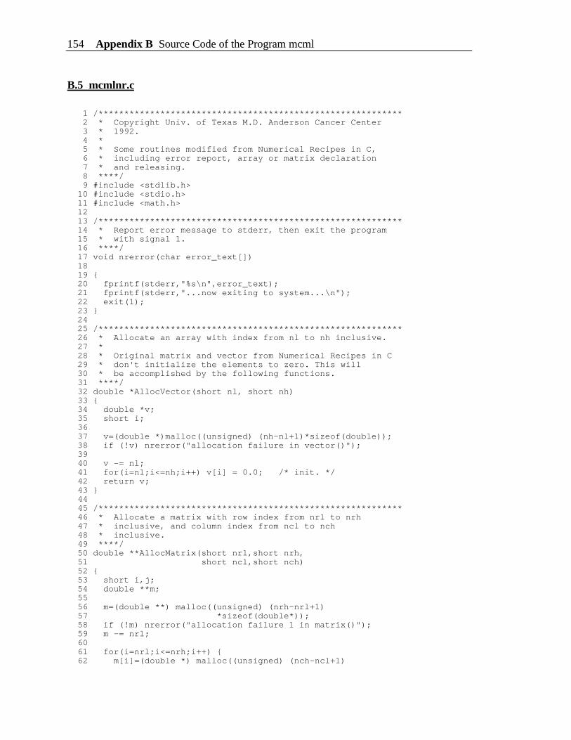
154 Appendix B Source Code of the Program mcml
B.5 mcmlnr.c
1 /*********************************************************** 2 * Copyright Univ. of Texas M.D. Anderson Cancer Center 3 * 1992. 4 * 5 * Some routines modified from Numerical Recipes in C, 6 * including error report, array or matrix declaration 7 * and releasing. 8 ****/ 9 #include <stdlib.h> 10 #include <stdio.h> 11 #include <math.h> 12 13 /*********************************************************** 14 * Report error message to stderr, then exit the program 15 * with signal 1. 16 ****/ 17 void nrerror(char error_text[]) 18 19 20 fprintf(stderr,"%s\n",error_text); 21 fprintf(stderr,"...now exiting to system...\n"); 22 exit(1); 23 24 25 /*********************************************************** 26 * Allocate an array with index from nl to nh inclusive. 27 * 28 * Original matrix and vector from Numerical Recipes in C 29 * don't initialize the elements to zero. This will 30 * be accomplished by the following functions. 31 ****/ 32 double *AllocVector(short nl, short nh) 33 34 double *v; 35 short i; 36 37 v=(double *)malloc((unsigned) (nh-nl+1)*sizeof(double)); 38 if (!v) nrerror("allocation failure in vector()"); 39 40 v -= nl; 41 for(i=nl;i<=nh;i++) v[i] = 0.0; /* init. */ 42 return v; 43 44 45 /*********************************************************** 46 * Allocate a matrix with row index from nrl to nrh 47 * inclusive, and column index from ncl to nch 48 * inclusive. 49 ****/ 50 double **AllocMatrix(short nrl,short nrh, 51 short ncl,short nch) 52 53 short i,j; 54 double **m; 55 56 m=(double **) malloc((unsigned) (nrh-nrl+1) 57 *sizeof(double*)); 58 if (!m) nrerror("allocation failure 1 in matrix()"); 59 m -= nrl; 60 61 for(i=nrl;i<=nrh;i++) 62 m[i]=(double *) malloc((unsigned) (nch-ncl+1)
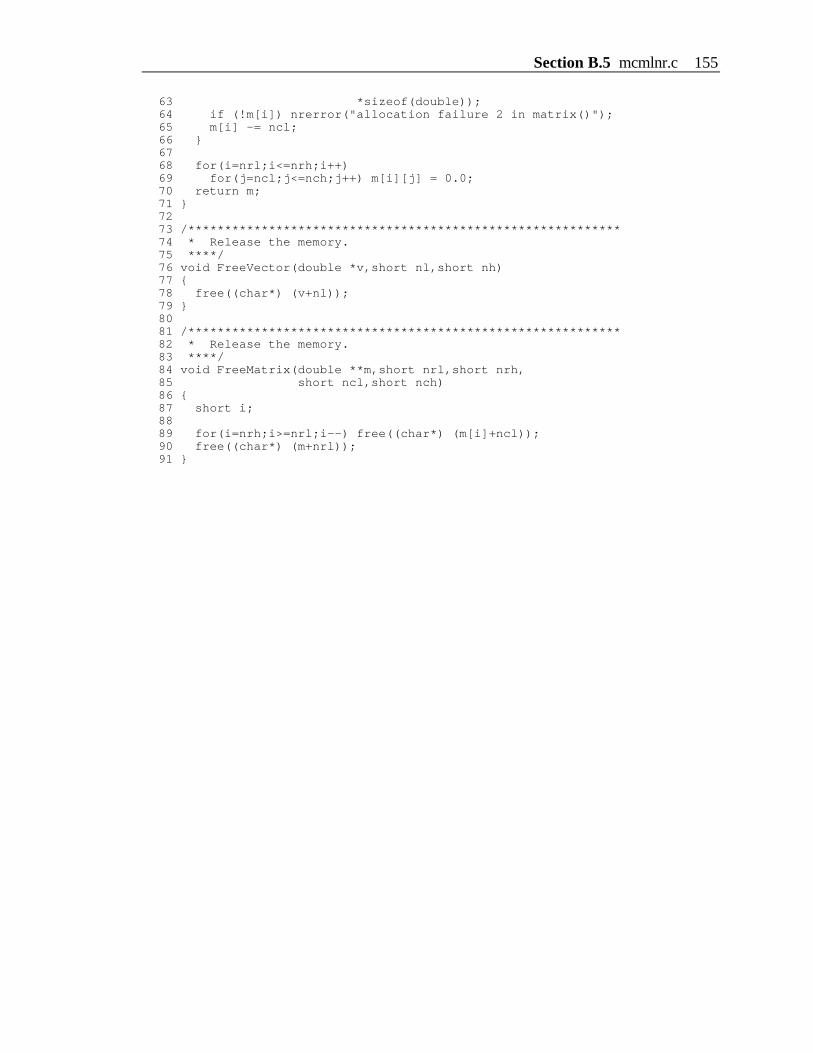
Section B.5 mcmlnr.c 155
63 *sizeof(double)); 64 if (!m[i]) nrerror("allocation failure 2 in matrix()"); 65 m[i] -= ncl; 66 67 68 for(i=nrl;i<=nrh;i++) 69 for(j=ncl;j<=nch;j++) m[i][j] = 0.0; 70 return m; 71 72 73 /*********************************************************** 74 * Release the memory. 75 ****/ 76 void FreeVector(double *v,short nl,short nh) 77 78 free((char*) (v+nl)); 79 80 81 /*********************************************************** 82 * Release the memory. 83 ****/ 84 void FreeMatrix(double **m,short nrl,short nrh, 85 short ncl,short nch) 86 87 short i; 88 89 for(i=nrh;i>=nrl;i--) free((char*) (m[i]+ncl)); 90 free((char*) (m+nrl)); 91

156 Appendix C Makefile for the Program mcml
Appendix C. Makefile for the Program mcml
We present the make file used for compiling and linking the code for UNIX users.
This make file (named makefile) can be placed under the same directory as the source
code, and used by the UNIX command make.
CFLAGS =CC=ccRM=/bin/rm -rfLOCAL_LIBRARIES= -lmOBJS = mcmlmain.o mcmlgo.o mcmlio.o mcmlnr.o
.c.o: $(RM) $@ $(CC) -c $(CFLAGS) $*.c#####
all : mcml
mcml: $(OBJS) $(RM) $@ $(CC) -o $@ $(OBJS) $(LOCAL_LIBRARIES)
clean:: $(RM) mcml $(RM) mcmlmain.o
If you use ANSI Standard C compiler (acc) on SPARCstation 2, you need to change cc to
acc in the second line. Similarly, if you want to use GNU C compiler, you need to use gcc
instead of cc. If you need to use a debugger (e.g., dbx), you need to add the option -g to
CFLAGS in the first line, and recompile the source codes using the new make file. Then,
you can call the debugger (e.g., dbx mcml). To compile and link use the makefile, use:
make

Appendix D A Template of mcml Input Data File 157
Appendix D. A Template of mcml Input Data File
This is a template for the input data file. The template file is named as
"template.mci" if nobody has changed its name. You can copy this file to a new file whose
extension is preferably ".mci", and modify the parameters in the new file to solve your
specific problem. Any valid filenames without spaces are acceptable (see Section 9.1 for
detail).
##### Template of input files for Monte Carlo simulation (mcml).# Anything in a line after "#" is ignored as comments.# Space lines are also ignored.# Lengths are in cm, mua and mus are in 1/cm.####
1.0 # file version2 # number of runs
### Specify data for run 1temp1.mco A # output filename, ASCII/Binary10 # No. of photons20E-4 20E-4 # dz, dr10 20 30 # No. of dz, dr & da.
2 # No. of layers# n mua mus g d # One line for each layer1.0 # n for medium above.1.3 20 200 0.70 0.01 # layer 11.4 10 200 0.90 1.0E+8 # layer 21.0 # n for medium below.
### Specify data for run 2temp2.mco A # output filename, ASCII/Binary20 # No. of photons20E-4 20E-4 # dz, dr80 80 30 # No. of dz, dr & da.
1 # No. of layers# n mua mus g d # One line for each layer1.0 # n for medium above.1.4 10 200 0.70 1.0E+8 # layer 11.0 # n for medium below.
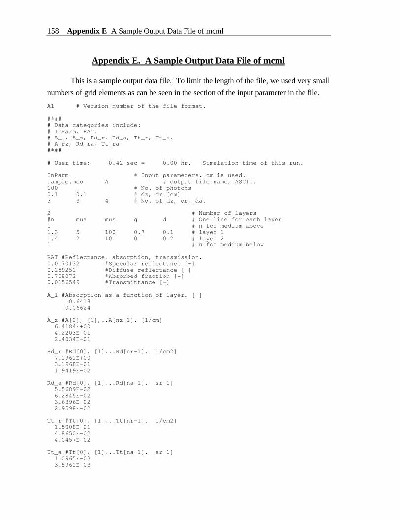
158 Appendix E A Sample Output Data File of mcml
Appendix E. A Sample Output Data File of mcml
This is a sample output data file. To limit the length of the file, we used very small
numbers of grid elements as can be seen in the section of the input parameter in the file.
A1 # Version number of the file format.
##### Data categories include:# InParm, RAT,# A_l, A_z, Rd_r, Rd_a, Tt_r, Tt_a,# A_rz, Rd_ra, Tt_ra####
# User time: 0.42 sec = 0.00 hr. Simulation time of this run.
InParm # Input parameters. cm is used.sample.mco A # output file name, ASCII.100 # No. of photons0.1 0.1 # dz, dr [cm]3 3 4 # No. of dz, dr, da.
2 # Number of layers#n mua mus g d # One line for each layer1 # n for medium above1.3 5 100 0.7 0.1 # layer 11.4 2 10 0 0.2 # layer 21 # n for medium below
RAT #Reflectance, absorption, transmission.0.0170132 #Specular reflectance [-]0.259251 #Diffuse reflectance [-]0.708072 #Absorbed fraction [-]0.0156549 #Transmittance [-]
A_l #Absorption as a function of layer. [-] 0.6418 0.06624
A_z #A[0], [1],..A[nz-1]. [1/cm] 6.4184E+00 4.2203E-01 2.4034E-01
Rd_r #Rd[0], [1],..Rd[nr-1]. [1/cm2] 7.1961E+00 3.1968E-01 1.9419E-02
Rd_a #Rd[0], [1],..Rd[na-1]. [sr-1] 5.5689E-02 6.2845E-02 3.6396E-02 2.9598E-02
Tt_r #Tt[0], [1],..Tt[nr-1]. [1/cm2] 1.5008E-01 4.8650E-02 4.0457E-02
Tt_a #Tt[0], [1],..Tt[na-1]. [sr-1] 1.0965E-03 3.5961E-03
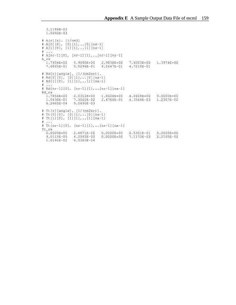
Appendix E A Sample Output Data File of mcml 159
3.1196E-03 1.5692E-03
# A[r][z]. [1/cm3]# A[0][0], [0][1],..[0][nz-1]# A[1][0], [1][1],..[1][nz-1]# ...# A[nr-1][0], [nr-1][1],..[nr-1][nz-1]A_rz 1.7934E+02 5.9590E+00 2.9838E+00 7.4003E+00 1.3974E+00 7.6865E-01 5.5296E-01 6.5647E-01 4.7210E-01
# Rd[r][angle]. [1/(cm2sr)].# Rd[0][0], [0][1],..[0][na-1]# Rd[1][0], [1][1],..[1][na-1]# ...# Rd[nr-1][0], [nr-1][1],..[nr-1][na-1]Rd_ra 1.7856E+00 2.0312E+00 1.8606E+00 4.0608E+00 0.0000E+00 1.0438E-01 7.3502E-02 2.4768E-01 4.3564E-03 1.2307E-02 8.2665E-04 5.0690E-03
# Tt[r][angle]. [1/(cm2sr)].# Tt[0][0], [0][1],..[0][na-1]# Tt[1][0], [1][1],..[1][na-1]# ...# Tt[nr-1][0], [nr-1][1],..[nr-1][na-1]Tt_ra 0.0000E+00 2.6871E-02 0.0000E+00 2.5301E-01 0.0000E+00 9.0115E-05 4.2593E-02 0.0000E+00 7.1173E-03 2.2105E-02 1.0191E-02 6.0383E-04

160 Appendix F Several C Shell Scripts
Appendix F. Several C Shell Scripts
F.1 conv.bat for batch processing conv
The C Shell script "conv.bat" is used to batch process the program conv (see
Section 9.4 for description of use of conv.bat).
# Shell script for the convolution program "conv"# Feb. 2, 1992## Format: conv.bat filename(s) output_type# output_type includes: Rr, Ra, Az ...
# Check parm, echo the help if something is wrong.if ($#argv == 0 || $#argv >= 3) then echo 'Usage: conv.bat "input_filename(s)" output_type' echo "output_type includes: " echo "I, 3, K" echo "Al, Az, Arz" echo "Rr, Ra, Rra" echo "Tr, Ta, Tra" exitendif
# Check the second parameter.if (! ($2 =~ [Ii3Kk] || \ $2 =~ [Aa][LlZz] || \ $2 =~ [Aa][Rr][Zz] || \ $2 =~ [RrTt][RrAa] || \ $2 =~ [RrTt][Rr][Aa])) then echo "Wrong parm -- $2" echo "output_type includes: " echo "I, 3, K" echo "Al, Az, Arz" echo "Rr, Ra, Rra" echo "Tr, Ta, Tra" exit(3)endif
foreach infile ($1) # make sure the file is existent and readable. if (! -e $infile) then echo "File $infile not exist" exit(2); else if (! -r $infile) then echo "File $infile not readable" exit(2) endif
# remove the existent output files, if any. if ( -e $infile:r.$2) then rm $infile:r.$2 endif
# echo the command sequence to conv. (echo i;echo $infile;\ echo oo;echo $2;echo $infile:r.$2;echo q;echo q;echo y)\ |conv>/dev/null
end # of foreach
Appendix F Several C Shell Scripts 161
F.2 p1 for pasting files of 1D arrays
The C Shell script p1 is used to paste side by side multiple files of 1D arrays,
which are in 2 columns. If the files of 1D arrays share the same first column, p1 will not
duplicate the first column in the pasted file. If the output file is existent, then it is backed
up as the original filename appended with ".bak". The original output file is still kept as
part of the new output file. This script is particularly useful to prepare the data for
processing and presentation by some commercial plotting softwares such as KaleidaGraph.
For example, if you have three mcml output files file1.Rr, file2.Rr, and file3.Rr saved in 2
columns representing the diffuse reflectance as a function of radius r. You can combine
these three files into one file by:
p1 "file?.Rr" filex.Rrs
where filex.Rrs is the filename of the output.
# Paste 1D files (in 2 columns) together side by side.# February 7, 1992.
# Check number of arguments.if ($#argv != 2) then echo 'Usage: p1 "input_file(s)" output_fname' exit(1)endif
onintr catch # Prepare to catch interrpts.
set com = $0set infiles = $1:qset outfile = $2
# Check validity of arguments for outfile.if ( -e $outfile) then if (! -w $outfile) then echo $outfile not writable exit(2) endif
cp $outfile $outfile.bak # Backup existent files.endif
# Setup temp files with the PID number.set outbuf = /tmp/$com:t.$$.outbufset buf1 = /tmp/$com:t.$$.buf1set buf2 = /tmp/$com:t.$$.buf2set cmp1 = /tmp/$com:t.$$.cmp1set cmp2 = /tmp/$com:t.$$.cmp2
# Run through each file, keep the results in $outbuf.foreach infile ($infiles) if (! -r $infile) then echo $infile not readable exit(3) endif

162 Appendix F Several C Shell Scripts
# Delimit by tab. awk -F" " 'print $1 "\t" $2' $infile >! $buf1
if (! -e $outbuf) then cut -f1 $buf1 >! $cmp1 cp $buf1 $outbuf else cut -f1 $buf1 >! $cmp2 diff $cmp1 $cmp2 > /dev/null
if ($status) then # 1st rows are not the same. Paste both columns. paste $outbuf $buf1 >! $buf2; cp $buf2 $outbuf cut -f1 $buf1 >! $cmp1 else # 1st rows are the same. Paste only the 2nd column. cut -f2 $buf1 >! $buf2 paste $outbuf $buf2 >! $buf1; cp $buf1 $outbuf endif endif
end
# Copy $outbuf to $outfileif (! -e $outfile) then cp $outbuf $outfileelse paste $outfile $outbuf >! $buf1; cp $buf1 $outfileendif
catch: # jump to here if interrupted rm -f $outbuf $buf1 $buf2 $cmp1 $cmp2 exit(1)

Appendix G Where to Get the Programs mcml and conv 163
Appendix G. Where to Get the Programs mcml and conv
We will eventually set up a bulletin board of our own so that you can download
the software over the network. For now, you can contact Lihong Wang, or Steven L.
Jacques using the following information to get the software.
Lihong Wang, Ph. D.
Laser Biology Research Laboratory – Box 17
University of Texas M. D. Anderson Cancer Center
1515 Holcombe Blvd.
Houston, Texas 77030
Phone: (713)745-1742
Fax: (713)792-3995
email: [email protected]
or
Steven L. Jacques, Ph. D.
Laser Biology Research Laboratory – Box 17
University of Texas M. D. Anderson Cancer Center
1515 Holcombe Blvd.
Houston, Texas 77030
Phone: (713)792-3662
Fax: (713)792-3995
email: [email protected]
Make sure that you tell us the specific machines (including brand and model) you will use
for the simulation, so that we can compile the code correctly for you. If you use IBM PC
compatibles, please also tell us whether you use a math co-processor or not.
164 Appendix H Future Developments of the Package
Appendix H. Future Developments of the Package
The release is by no means the end of the package. We plan to make at least the
following improvements. As we gather comments from users, we may consider even more
improvements.
Collimated responses in mcml
In this version (version 1.0) of mcml, the first photon interactions in the media are
scored into the first grid elements in the r direction together with the later interactions.
The first interactions are all on the z-axis, and should yield a delta function of r (Gardner
et al., 1992b) to be exact. Therefore, they should be scored separately as demonstrated by
Gardner et al.
The specular reflectance is computed analytically using Fresnel's formulas.
However, the reflected photons that are uninteracted inside the tissue are scored into the
first grid elements in the r direction of the diffuse reflectance. To be strict, these photons
should contribute to the specular reflectance rather than the diffuse reflectance although
this is small in thick tissues.
The transmittance in version 1.0 of mcml does not differentiate between diffuse
transmittance and unscattered transmittance. This problem and the problem with the
reflectance can be solved by keeping track of the number of interactions.
Best points for each grid element
As we have discussed in Section 4.3, we should use:
rb = [(n + 0.5) + 1
12 (n + 0.5) ] ∆r
instead of the center of the grid element as the coordinate of the simulated data in the nth
grid element in the r direction. In the case when the radius of a Gaussian beam is
comparable with the grid separation ∆r, this may make a considerably large difference in
the convolution program conv.

Appendix H Future Developments of the Package 165
Flexible photon sources
In version 1.0 of mcml, only collimated photon beams incident on the tissue
surface are supported. Several other cylindrically symmetric sources should be able to be
incorporated without substantially modifying the program.
The convolution program conv 1.0 only supports Gaussian beams and circularly
flat beams, it can be easily adopted to convolve over arbitrary beam profiles that are
cylindrically symmetric. For beams that are not cylindrically symmetric, the convolution
still can be done but with longer integration time.
Faster sampling procedures
The sampling of the step size involves an exponential computation which is
computation intensive. Faster approaches can be used as discussed in Section 3.2.

166 References
References
Ahrens, J.H. and U. Dieter, "Computer Methods for Sampling for the Exponential and
Normal Distributions," Comm. ACM, 15, 873 (1972).
Anderson, G., and P. Anderson, "The UNIX C Shell Field Guide," Prentice-Hall (1986).
Arthur, L.J., "UNIX Shell Programming," Second Ed., John Wiley & Sons, Inc. (1990).
Born, M., and E. Wolf, "Principles of Optics: Electromagnetic Theory of Propagation,
Interference and Diffraction of Light," Sixth corrected Ed., Pergamon Press (1986).
Cashwell E.D., C.J. Everett, "A Practical Manual on the Monte Carlo Method for
Random Walk Problems," Pergamon Press, New York (1959).
Cheong W.F., S.A. Prahl, A.J. Welch, "A Review of the Optical Properties of Biological
Tissues," IEEE J Quantum Electronics, 26, 2166-2185 (1990).
Gardner, C.M., and A.J. Welch, private communication, Biomedical Eng. Program, Univ.
of Texas, Austin (1992).
Gardner, C.M., and A.J. Welch, in SPIE Proceedings, Laser-tissue Interaction III, Vol.
1646 (1992b).
Giovanelli, R.G., "Reflection by Semi-Infinite Diffusers," Optica Acta, 2, 153-162 (1955).
Hecht, E., "Optics," Second Ed., Addison-Wesley Publishing Company, Inc. (1987).
Hendricks, J.S., and T.E. Booth, "MCNP Variance Reduction Overview," Lecture Notes
in Physics, 240, 83-92 (1985).
Henyey, L.G., and J.L. Greenstein, "Diffuse Radiation in the Galaxy," Astrophys. J., 93,
70-83 (1941).
Kalos, M.H., and P.A. Whitlock, "Monte Carlo Methods, I: Basics," John Wiley & Sons,
Inc. (1986).

References 167
Keijzer, M., S.L. Jacques, S.A. Prahl, and A.J. Welch, "Light Distributions in Artery
Tissue: Monte Carlo simulations for Finite-Diameter Laser Beams," Lasers in Surg. &.
Med., 9, 148-154 (1989).
Kelley, A., and I. Pohl, "A Book on C: Programming in C," Second Ed.,
Benjamin/Cummings Publishing Company, Inc. (1990).
Lux, I., and L. Koblinger, "Monte Carlo Particle Transport Methods: Neutron and Photon
Calculations," CRC Press (1991).
MacLaren, M.D., G. Marsaglia, and T. Bray, "A Fast Procedure for Generating
Exponential Random Variables," Comm. ACM, 7, 298 (1964).
Marsaglia, G., "Generating Exponential Random Variables," Ann. Math. Stat., 32, 899
(1961).
Plauger, P.J., and J. Brodie, "Standard C," Microsoft Press (1989).
Prahl, S.A., "Calculation of Light Distributions and Optical Properties of Tissue," Ph.D.
Dissertation, Department of Biomedical Engineering, U. Texas at Austin (1988).
Prahl, S.A., M. Keijzer, S.L. Jacques, and A.J. Welch, "A Monte Carlo Model of Light
Propagation in Tissue," Dosimetry of Laser Radiation in Medicine and Biology, SPIE
Institute Series, IS 5, 102-111 (1989). (Note the typo in Eq. (10), where the denominatorshould be 1 – g0 + 2 g0 ξ).
Press, W.H., B.P. Flannery, S.A. Teukolsky, and W.T. Vetterling, "Numerical Recipes in
C," Cambridge Univ. Press (1988).
Spiegel, M. R., "Mathematical Handbook of Formulas and Tables," McGraw-Hill, Inc.,
(1968).
Symantec Corporation, "THINKC User Manual," Symantec Corporation (1991).
van de Hulst, H.C, "Multiple Light Scattering, Volume II," Academic Press, New York
(1980).
Wang, L.-H., and S.L. Jacques, "Hybrid Model of Monte Carlo Simulation Diffusion
Theory for Light Reflectance by Turbid Media," unpublished.

168 References
Wilson, B.C., and S. L. Jacques, "Optical Reflectance and Transmittance of Tissues:
Principles and Applications," IEEE J. of Quant. Electronics, 26 (12), 2186-2199 (1990).
Witt, A.N., "Multiple Scattering in Reflection Nebulae I. a Monte Carlo approach," The
Astrophysical J. Supp. Series, 35, 1-6 (1977).
Wyman, D. R., M. S. Patterson, and B. C. Wilson, "Similarity relations for anisotropic
scattering in Monte Carlo simulations of deeply penetrating neutral particles," J. Comput.
Phys., 81, 137-150 (1989a).
Wyman, D. R., M. S. Patterson, and B. C. Wilson, "Similarity relations for the interaction
parameters in radiation transport," Appl. Opt., 28, 5243-5249 (1989b).
Index 169
Index
A, 37
A_l, 37, 95
A_rz, 36, 96
A_z, 36, 95
absorption, 4
absorption, 15, 24, 37
absorption coefficient, 35
absorption coefficient, 4, 5, 25
Absorption coefficient, 92
absorption-only, 30
angularly resolved diffuse reflectance and
transmittance, 48
anisotropy, 16
anisotropy, 4
anisotropy factor, 35
ANSI C, 87
ANSI Standard C, 87, 91
ANSI Standard C, 32
Apple Edit, 91
arrows, 14
ASCII format, 92
AXUM, 96
azimuthal angle, 15
background job, 95
background processes, 95
batch process, 96
Bessel function, 71, 76
binary files, 91
binary tree, 74
binary tree, 77
bit bucket, 95
Boolean, 35
bugs, 97
buried isotropic photon sources, 110
Cartesian coordinate system, 5
cell, the last, 22
cflow, 41
CHANCE, 33
comment lines, 91, 95
compress, 90
computation results, 47
computation time, 52
constants, 33
contour, 66
Contour, 83
conv, 80
convolution, 67
convolution, 67
convolution error, 85
convolve, 96
coordinate systems, 5
cos_crit0, 35
cos_crit1, 35
COS90D, 33
COSZERO, 33
critical angles, 35
cross the boundary, 38
cumulative distribution function, 7
cylindrical coordinate system, 5
da, 36
Data structures, 34
dead, 34
deflection angle, 15
delta function, 30
depth resolved internal fluence, 50
diffuse reflectance, 22, 37
170 Index
diffuse reflectances, 63, 81, 84
diffuse transmittance, 48
diffuse transmittance, 19
dimensional step size, 14
dimensionless step size, 14
directional cosines, 17
directional cosines, 11, 34
divergence, 71
dr, 36
duplicated filenames, 43
dynamic allocation, 37
dz, 36
editor, 91
eject, 88
electronic mail, 89
EMACS, 91
empirical formulas, 55, 58
empirical formulas, 62
Ethernet, 97
execution, 93
extended trapezoidal integration, 31
extended trapezoidal integration, 74
extraction, subset, 96
extrapolations, 76
file expansion, 97
file format, 92
file of input data, 91
file of output data, 95
File version, 92
filename for data output, 36
first photon interactions, 30
flat beam, 69
flat beams, 72
flow graph, 41
flow of the program, 32
flowchart, 38
fluences, 65, 82, 85
folder, 96
folder, 94
free path, 12
Fresnel reflectances, 12
Fresnel's formulas, 18
FTP, 91, 97
g, 35
Gaussian beam, 69
glass, 12
glass layer, 14, 38
GNUCC, 33
grid line separations, 92
grid system, 5
Henyey and Greenstein, 15
hybrid model, 55
IBM PC compatibles, 94
implicit photon capture, 11
impulse response, 67
impulse response, 66
index range of the array, 37
input data file, 91, 97
input parameters, 35, 95, 97
InputStruct, 36
instructions, 91
integers, 97
integral limits, 77, 79
integrand evaluation, 76, 78
intensity profile, 68
interaction coefficient, 4, 12, 40
interpolations, 76
invariance, 67
isotropic photon sources, 110
isotropic photon sources, buried, 110
job, background, 95
KaleidaGraph, 161
Index 171
KaleidaGraph, 96
Kermit, 91
KERMIT, 97
last cells, 22
Launch photon, 38
layer, 34
Layer parameter, 93
layerspecs, 36
LayerStruct, 35
linear and invariant, 67
linear approximations, 27
linear linked list, 43
linearity, 67
logarithmic operation, 45
log-log plot, 55
log-log scale, 55
long int, 36
Macintosh, 94
mail, 90
mails, 89
make file, 32
matched boundaries, 53
matched boundary, 47
Max, 78, 79
Max, 72
mean free path, 93
mean free path, 13
Mean free path, 2
mean free path, transport, 52, 111
memory, iii, 37, 43, 93
memory, release, 43
Microsoft Word, 91
Min, 78, 79
mismatched boundaries, 58
mismatched boundary, 48
mismatched boundary, 11
MockWrite, 91
modem, 97
modified Bessel function, 71
modify the program, 110
Monte Carlo, 1
mua, 35
multi-layered tissue, 4
multi-layered tissues, 62
multiple runs, 93
multiple simulations, 43
mus, 35
n, 35
na, 36
nesting depth, 41
network, 91
Norton editor, 91
nr, 36
num_layers, 36
num_photons, 36
Number of grid elements, 93
Number of layers, 93
number of photon packets, 36
Number of photon packets, 92
Number of runs, 92
numerical computation, 73
nz, 36
observation point, 68
operating system, 91
out_fformat, 36
out_fname, 35
output data files, 95
Output filename, 92
OutStruct, 37
overflow, 77
overflow, 22
partial reflection approach, 19
172 Index
PARTIALREFLECTION, 33
path, search, 94
photon absorption, 15
photon fluence, 25
photon packet, 11, 34
photon propagation, 11
photon scattering, 15
photon termination, 20
PhotonStruct, 34
physical quantities, 4, 22
position of the photon packet, 14
probability density function, 7
probability of interaction, 12
process, background, 95
profiler, 44, 46
pseudo-random number generator, 7
radially resolved diffuse reflectance, 49
random variable, 7
RAT, 95
Rd, 36
Rd_a, 36, 95
Rd_r, 36, 95
Rd_ra, 36, 96
real time, 43
reflectance, 18
reflection at boundary, 17
reflection at interface, 19
refractive index, 35
Refractive index, 93
release the memory, and continues
execution, 43
resolution, 92
roulette, 36
roulette, 20, 41
Rsp, 36
s, 34
sampling random variables, 7
scattering coefficient, 35
scattering coefficient, 4, 5, 92
scattering function ), 15
script file, 96
search path, 94
search path, 88
semi-infinite turbid medium, 47
shell programming, 96
short, 35
similarity relations, 50, 111
sleft, 34
Snell's law, 18
software installation, 87
solid angle, 23, 48
source, 68
source code, 32
source or error, 79
source point, 68
space lines, 91, 95
specular reflectance, 37, 95
specular reflectance, 12, 22
spherical coordinate system, 5
standard errors, 47
STANDARDTEST, 33
step size, 12, 35
STRLEN, 33
subset extraction, 96
subset of the output data, 96
tar, 90
Taylor series, 28
template file, 91
termination, 20
text editors, 91
text format, 91
THINKCPROFILER, 33
Index 173
threshold weight, 36
time of computation, 52
timer, 97
time-shared system, 53
timing profile, 43
Timing profile, 45
tissue/tissue interface, 19
total absorption, 95
total diffuse reflectance, 95
total diffuse reflectance, 37, 47, 48
total diffuse reflectance and
transmittance, 23
total diffuse transmittance, 48
total transmittance, 95
total transmittance, 47
trajectory, 2
transformation of variables, 69
transmission at boundary, 17
transmission at interface, 19
transmittance, 18
transmittance, 22
transmittances, 63
transmittances, 82, 84
transport mean free path, 52
transport mean free path, 111
trapezoidal rule, 73
Tt, 37
Tt_a, 37, 95
Tt_r, 37, 95
Tt_ra, 37
Tt_ra, 96
uncompress, 89
unit of length, 5
UNIX, 94
unscattered transmittance, 19
unscattered transmittance, 48
user time, 43, 95, 97
user times, 52
uudecode, 89
uuencode, 90
ux, 34
uy, 34
uz, 34
variance, 92
variance reduction technique, 11
vi, 91
w, 34
wave phenomenon,, 2
weight, 11
wild cards, 97
Word, 91
Wth, 36
x, 34
y, 34
z, 34
z0, 35
z1, 35