Embed Size (px)
Citation preview

1
Monte Carlo ray tracing in optical canopy reflectance modelling
M. I. Disney1*, P. Lewis1, P. R. J. North2
Abstract
This paper reviews the use of Monte Carlo methods in optical canopy reflectance modelling. Their
utility, and, more specifically, Monte Carlo ray tracing for the numerical simulation of the radiation
field within a vegetation canopy, are outlined. General issues pertinent to implementation and
exploitation of such methods are discussed, such as the descriptions of canopy structure and
radiometric properties required for their use. Strategies for the reduction of variance, which form the
core of the application of Monte Carlo methods to canopy reflectance modelling are presented, and
examples given of the type of information which may be obtained from canopy reflectance modelling
using Monte Carlo ray tracing. The use of Monte Carlo methods in the development of models of
canopy development, driven by fundamental properties such as radiation interception are discussed.
Keywords: Monte Carlo ray tracing, canopy reflectance modelling.
1 Remote Sensing Unit, Department of Geography, University College London, 26 Bedford Way, London WC1H 0AP,UK2 Institute of Terrestrial Ecology, Monks Wood, Abbots Ripton, Huntingdon, Cambs., PE17 2LS, UK
*corresponding author. Email: [email protected]
Review article submitted for publication in Remote Sensing Reviews (International Forum onBRDF Special Issue)
Manuscript received 17/10/99 ; revised 30/11/99_
2
1. INTRODUCTION
A wide range of physically based models have been developed to describe the scattering of
shortwave radiation by vegetation canopies (Goel, 1988; Goel and Thompson, 2000). Although
various analytical models have been developed which describe overall effects of canopy biophysical
parameters on scattering and absorption, such approaches are limited in the complexity of the scene
description that can be used (Myneni et al., 1989). Analytical models are also heavily reliant on the
validity of various sets of assumptions and simplifications employed to make the problems more
tractable (Pinty and Verstraete, 1998). Whilst these models have a key role to play in describing
generalised behaviour, and appear to mimic canopy reflectance reasonably well in many cases, their
application is ultimately limited to homogeneous or relatively simple heterogeneous scenes on flat or
constantly sloping terrain. Although multiple spatial scales can be considered in such models (Hapke,
1984; Lumme and Bowell, 1987), the resulting models are again limited to relatively simple
scenarios. In addition, changing the scene geometry (e.g. spatial distribution of the plants in a
heterogeneous scene) or the assumptions made in defining the model generally requires a significant
re-working of the formulae. Analytical models have the advantage of being fast to calculate, a
property which, along with their use of generalised parameters, has in the past made them suitable
candidates for non-linear numerical inversion schemes which require repeated forward modelling
(Kuusk, 1996). Recent developments in the use of look-up table (LUT) inversion methods
somewhat reduce the emphasis on speed of canopy reflectance calculation, however, in that the
elements of the LUT can be pre-computed (i.e. calculated once only) (Knyazikhin et al., 1998).

3
A more flexible approach to modelling canopy scattering can be taken by reducing the problem of
computing canopy reflectance to five main elements (Lewis, 1999):
(i) description of the structure of the scene elements (plants, soil, topography);
(ii) description of the scattering properties of the scene elements (reflectance, transmittance of
leaves, stems etc.);
(iii) description of the illumination conditions (sun angle, atmospheric conditions);
(iv) description of sensor imaging characteristics (spectral characteristics, scanning
characteristics, motion);
(v) numerical solution for radiation transport between the illuminator and the sensor via
interactions with the scene elements.
This is not intended to dictate a blueprint for an ‘ideal’ model of canopy reflectance. Rather they are
proposed as a framework for the discussion of the major issues which must be considered when
developing models of this sort. The relative importance attached to these points in any particular
implementation will inevitably be driven by the application for which the model is developed.
A limitation of the description given above is that it is static. More desirable still is the development
of models which actually operate as a function of environmental properties such as light, water, and
nutrient availability etc. This allows an integrated aproach to, and link between, radiometric
simulation and other process models (e.g. canopy growth and development, water and energy usage
etc.). Such a model can be considered, in effect, as a ‘virtual laboratory’ (Prusinkiewicz and
Lindenmayer, 1990) which allows a much richer exploration of the remote sensing signal and the
4
development of appropriate methods for mapping vegetation parameters from Earth Observation
data. This type of approach will not replace more traditional field-based and other measurement
studies however, nor will it replace established analytical modelling strategies: such a generic model
is typically driven by a very large number of parameters, rendering inversion impracticable for the
most part. Such models can however be used in the forward mode to test the impact of the
approximations made in other, less complex models (Govaerts 1996; Kuusk et al., 1997; Disney and
Lewis, 1998). This is discussed in greater detail in section 4.
Progress is being made towards the type of generic model described above from various quarters,
driven in part by cheaper, faster computers, computer graphics (CG) algorithms, and the rapidly-
emerging field of 3D plant measurement and modelling (Prusinkiewicz, 1999). The latter
developments lead to the possibility of representing canopy structure as accurately as required,
through 3D scanning methods (Room et al., 1996), stereo-photogrammetry (Lewis and Boissard,
1997), manual measurements (Lewis, 1999), algorithmic growth models such as that of
Prusinkiewicz and Lindenmayer (1990) or models driven by botanical growth rules (De Reffye et al.,
1997) . Prusinkiewicz (1996), and M•ch and Prusinkiewicz (1996) discuss the application of L-
system-based models of plant growth in areas such as ecology and epidemiology. Fournier and
Andrieu (1999) have developed a model that couples canopy organ growth as a function of
temperature and carbon availability to 3D spatial variations of light and temperature within the
canopy. Chelle and Andrieu (1999) describe a range of recent developments in the coupling of
numerical solutions of radiation transport within canopy radiation models to physiologically-based
models for the purpose of characterising canopy development as a function of incident radiation.
The LIGNUM model of Perttunen et al. (1996) is another approach to the construction of process
5
models of plant growth (trees in this case). LIGNUM is an attempt to simplify the treatment of
metabolic functions controlling growth in the context of structurally detailed 3D plant models.
A key component in this concept of a generic remote sensing model is element (v) described above
i.e. a numerical solution for radiation transport. If the numerical solution is flexible enough, this
modular approach can be used to simulate scattering under a much wider range of conditions than is
possible using analytical methods. Crucially, for remote sensing simulations, this approach is
appropriate to scene simulation at a wide range of spatial scales and wavelength domains. To
provide the most flexible model, the number of assumptions made about the nature of radiation
transport should be kept to a minimum. For example, geometric optics (GO) theory, useful in the
visible and thermal domains (size of scattering elements >> λvis, thermal), is not generally appropriate at
microwave wavelengths. Additionally, simulations at thermal wavelengths requires the scene
elements themselves to be considered as source of ’illumination’ (thermal radiation), and transport is
further complicated by air mass movements. Whatever approach used, the generic model should
comply with fundamental laws of physics, such as the conservation of energy.
In general, radiative transfer models treat the canopy (or parts of the canopy) as a set of statistical
ensembles defined over a volume with averaged properties or distribution functions (e.g. leaf angle
distribution), and are solved using appropriate radiative transfer approaches (Pinty and Verstraete,
1998). The ‘volumetric medium’ may be defined as a slab of infinite horizontal extent, or bounded
by some simple geometric form, such as a spheroid or cylinder (Begué, 1992). More flexibly, it may
be defined as regular gridded 3D ('voxel') cells, such as in the DART model of Gastellu-Etchegorry
et al. (1996), an adaptation of the model of Kimes and Kirchner (1982). This approach is attractive

6
in that relatively few parameters are required for description of the system, whilst a degree of spatial
fidelity is maintained. Further, it is also possible to make approximations to account for spatial
aspects such as finite leaf size and the resultant hot-spot effect (Myneni et al., 1991). However all
approxmiations made regarding the averaged scattering behaviour of the canopy must be accepted
as generalisations. There will be an inherent loss of information resulting from the assumption that
averaging canopy structural properties, and removing any explicit spatial linkages between them will
provide the same scattering behaviour as averaging the scattering behaviour of the ‘full’ 3D
situation.
A more general approach is to consider interaction of radiation with canopy elements defined in a
deterministic manner from the outset. The simulated signal can then be described as an average of all
such interactions. This approach requires an explicit 3D description of the location, orientation, size
and shape of each scatterer. Whilst various numerical methods exist for treatment of scattering
within and from a volumetric medium (Myneni et al., 1988), methods which are appropriate to both
‘volumetric and deterministic’ canopy definitions can largely be grouped into two approaches: (i)
radiosity methods; (ii) ray tracing methods. In the former, using an approach adapted from thermal
engineering, a ‘view factor’ matrix is constructed which represents the projection of each scattering
surface onto every other surface within a scene (Cohen and Wallace, 1993). The matrix is then used
in an iterative manner to solve for radiation scattered between all surfaces. Radiosity methods are
widely used in computer graphics for realistic scene rendering, and have also found application in
canopy reflectance modelling (Borel et al., 1991; Goel et al., 1991). A major advantage of the
method is that once a solution is found for radiative transport, canopy reflectance can be simulated
at any view angle. Although various acceleration methods can be applied, a major limitation of the

7
method is the initial computational load in forming the view factor matrix and solving for radiative
transport. This is particularly true for very complex scenes involving a large number of scattering
primitives. However, radiosity remains a useful technique in scenes characterised by a relatively
simple set of primitives.
Ray tracing methods are based on a sampling of photon trajectories within the scene. The processing
time required for this does not increase so dramatically as the scene complexity increases, and ray
tracing can therefore provide a more ‘scaleable’ generic solution for radiative transport. Ray tracing
methods are useful for a wide variety of radiation transport problems, and are the only really
appropriate methods for applications where path length is specifically required, for example in
modelling LiDAR (Light Detection And Ranging) (Govaerts, 1996; Lewis, 1999) or for SAR
interference effects (Lin and Sarabandi, 1999). The key to effective use of ray tracing methods is the
application of effective sampling schemes. The basis for the selection of photon trajectories and
various other aspects of ray tracing is the Monte Carlo method. This paper discusses the role of
Monte Carlo methods in ray tracing models of canopy reflectance in the context of the five points
outlined above, and the various options available in the implementation of such a model.
2 MONTE CARLO METHODS
Monte Carlo (MC) methods form a simple, robust and powerful set of tools for solving large multi-
dimensional problems by stochastically sampling a probability density function characterising the
behaviour of the system under investigation (Halton, 1970). As the number of samples of the
8
system increases, convergence toward a solution is achieved at a rate of n-1/2 for n samples. As a
result, it is important to strike a balance between a solution that is sufficiently accurate for the
requirements of the problem in hand, whilst using the smallest number of samples possible. The
rate at which the scheme converges also depends on the expected variance in the system, but
effective ‘variance reduction’ methods can improve performance dramatically (ibid.). MC methods
are particularly attractive for multi-dimensional sampling problems because increasing the
dimensionality of the problem does not dramatically increase the solution time. In addition, a
minimum of assumptions regarding the system under investigation are required. As a result, MC
(stochastic) simulation methods have been widely applied in cases where numerical solutions to
highly complex systems are required, such as satellite design (Klinkrad et al., 1990), stellar
evolution (Spurzem and Giersz,1996) and VLSI design (Keramat and Kielbasa, 1997) among many
other areas.
MC techniques are inherently suited to describing the scattering behaviour of photons however, as
this is an intrinsically stochastic event: the scattering phase function simply being the probability
density function for scattering at a particular angle (Myneni et al., 1989). It is therefore not
surprising that such methods have been applied to modelling canopy reflectance. Describing
vegetation canopy reflectance can be considered as a complex, multi-dimensional integral problem.
The solution requires sampling over the spatial, angular, and, for broadband sensor simulations,
wavelength domains. It is therefore an appropriate application for MC methods. Myneni et al.
(1989; pp 96-98) provide a brief review of MC methods in canopy reflectance modelling prior to
1989. Lenoble (1985) provides more detailed information on much of this and related material.

9
Estimation of flux can be regarded as the integrated sum of light transmitted across all possible
paths between source and receiver. Monte Carlo methods can be used to perform this integral by
sampling the possible photon trajectories. Alternatively, considering reflectance as the sum of
contributions of facets visible from a certain viewpoint, Monte Carlo methods can be used to
sample the global illumination on each facet, which allows accurate formation of an image
accounting for multiple scattering from the source. The equation governing the transfer of spectral
radiance from an illumination source of wavelength λ in direction Ω’ scattered towards a viewer in
direction Ω by one side of an elemental surface Aδ is given by:
∫ +ΩΩ⋅ΩΩΩ=Ω
πλλλ
2’’)’,,()’,(),( dNfLL ie (1)
where eL is the radiance leaving the surface, iL is the radiance incident on the surface, N is the unit
normal vector of the surface over Aδ , and )’,,( ΩΩλf is the spectral bidirectional reflectance
distribution function (BRDF). Equation (1) is often called the reflectance equation (Wallace and
Cohen, 1993), and can be stated in a number of (equivalent) ways (e.g. the rendering equation of
Kajiya (1986)). MC techniques provide an estimate of eL from equation (1) by transforming the
integral to an equivalent infinite series summation equation, and randomly sampling the population
of the summation for interactions between all surfaces in a scene. The problem is expressed as
(Halton, 1970):
[ ] ( )∫= )(ξµξττ dE (2)

10
where τ is known as the primary estimator of the solution (a function of some variable ξ), and
[ ]τE is the expected value of the integral. Using the MC method to evaluate equation (1), it is
important to select a primary estimator for eL so as to make the variance of the primary estimator
[ ]τvar as small as possible. For m samples of τ :
[ ] [ ]τvar)/1(,var mmLe = (3)
Note that the solution for canopy radiance or reflectance requires that the integral is solved for
energy transfer between all scatterers in the scene. MC methods allow this total set of interactions
to be simulated by sampling a limited number of interactions.
The key to efficient MC sampling then, is to use an understanding of the major effects within a
system to keep the expected variance in the sampling to a minimum, whilst utilising a minimum
number of samples. One example of this would be the evaluation of the integral of a BRDF by
biasing sampling to equal samples over weighted solid angle sectors, where the weighting is
provided by a similar, but simpler function. Variance reduction can be said to be the core of MC
methods, particularly in the case of application to complex physical models. This is discussed in
greater deatil in section 3. In practice, MC algorithms require a large number of samples of the
system in question in order to converge to a solution. The MC method will, of course, provide a
stochastic simulation and will always contain statistical variations (noise in the simulation), which
might be considered as a disadvantage. This argument can be turned on its head however, in that
the potential for deriving an understanding of the (random) error in the simulation as a side-effect
11
of the simulation process can be considered a major advantage of the method over other numerical
methods, which will never, in any case provide exact solutions.
3 MONTE CARLO RAY TRACING
3.1 Fundamental options in using MCRT
In simulating canopy reflectance, MC methods allow the multi-dimensional integral (over
wavelength, spatial and angular domains) involved to be reduced to a repeated sampling of a much
simpler set of interactions. Intuitively, the intrinsic canopy reflectance, the canopy BRDF, is
considered as an averaged probability of a sample set of photons (or rays in the direction of a
wavefront, “fired” into a scene) being incident on the canopy from a given direction and leaving per
unit solid angle around another direction. Alternatively, the bi-directional reflectance factor (BRF)
can be considered as the probability of photons incident from a given direction leaving in another,
relative to their behaviour when scattered by a perfect Lambertian horizontal reflecting surface.
Similarly, terms related to angular integrals of BRDF under varying illumination conditions, such as
the directional-hemispherical and bi-hemispherical reflectance (DHR and BHR) can be calculated as
appropriate angular integrals of photon probabilities. The effects of complex illumination or sensor
conditions can be easily integrated into such an approach by considering appropriately weighted
photon probabilities.
12
MC methods are most commonly employed in the simulation of canopy reflectance through Monte
Carlo Ray Tracing (MCRT). Using the intuitive approach outlined above, the aim is to calculate the
required probabilities by simulating the firing of photons into a scene. Within a given constant
density medium, a ray, describing a photon trajectory (or alternatively, the direction of propagation
of an electromagnetic wave), will travel along a straight line. Consequently, the main computational
issue becomes one of testing the intersection of a set of lines (rays) with a defined scene geometric
representation. For canopy reflectance modelling, the scene will typically include a lower (ground)
boundary, so a ray travelling from a virtual sensor into the scene will intersect with either a
vegetation or a ground element. At this point, the photon is either scattered (reflected or
transmitted) or absorbed, i.e. the sum of the probabilities of reflectance (Pr), transmittance (Pt), or
absorptance (Pa) equal unity. The integral over all conditions can be simulated using the MC
approach by generating a random number ℜ over the interval (0,1]. If ℜ is less than or equal to Pa,
then the photon is absorbed. If ℜ is between Pa and Pa + Pr, the photon is reflected (i.e., scattered
from the same side of the object that the path was initially incident upon). Otherwise, the photon is
transmitted. In the latter two cases, the BRDF of the scattering primitive (e.g. leaf reflectance
function) is used as a probability density function to relate another random number to a scattering
direction. The trajectory of the scattered photon is then followed until interception by another
primitive, or the photon escapes the scene. As noted above, a useful generic numerical model should
rely on as few assumptions as possible. Govaerts (1996) summarises the assumptions underlying a
model such as that described as:
(i) light propagation can be described using geometric optics;
13
(ii) incident radiation can be simulated with a finite number of non-interacting rays;
(iii) quantum transitions and diffraction can be ignored;
(iv) the structural properties of the medium can be described with geometric primitives;
(v) optical scattering properties can be defined with probability density functions.
An MCRT scheme of this sort was implemented in the models of Cooper and Smith (1985) (for soil
reflectance), Dauzat and Hautecoeur (1991), and Govaerts (1996). The model has the advantage of
being functionally simple and intuitive. Since the method relies on tracking photon fates, energy
conservation is ensured. In addition, absorptance by the scene elements is calculated at the same
time as canopy reflectance. This can be used, for instance, to calculate the amount or proportion of
photosynthetically-active radiation (PAR) absorbed by a canopy, which in turn provides the major
driver to process-based models of plant growth through conversion of absorbed PAR (APAR) to
assimilates (Fournier and Andrieu, 1999).
Although this approach to using MCRT offers many advantages, it suffers from the drawback that
absorption events involve a termination to a photon path and contribute to the simulation of the
BRDF only through their absence. If the purpose of a simulation is the calculation of the BRDF, this
involves necessary but ‘wasted’ processing time as a photon which ends up being absorbed by the
canopy or soil may have undergone several interactions with canopy and soil elements before
absorption. Also, since scattering and absorption properties generally vary as a function of
wavelength, multispectral simulation is generally costly as new rays must be traced for each
wavelength (or waveband) considered. One way to overcome this is considered by Cooper and
Smith (1985) in simulating soil reflectance. They considered the reflectance function to be
14
Lambertian, and the same for all primitives (ρ). Total reflectance Aρ can then be decomposed into an
infinite series:
Aρ = ρA1 + ρ2A2 + ρ3A3 + … (4)
Finding the solution for Aρ then involves solving for all ‘geometric’ terms Ai and using appropriate
values of ρ for each waveband. The terms Ai are due to combined geometric effects for scattering
order I and are calculated by storing the signal as a function of scattering order. Although they use a
rather different MC model to achieve this, Lewis and Disney (1998) calculate a similar set of
geometric terms, analogous to Ai for interactions between soil and vegetation. They go on to note
that these geometric attenuation terms are generally well-behaved and can be approximated by
simple functional forms:
Aρ = Aρ/(1-Bρ) (5)
This ‘geometric’ formulation, in particular the product of the geometric attenuation term B and
reflectance ρ in equation (5), turns out to be very closely-related to the maximum eigenvalue of the
radiative transport equation (Knyazikhin et al., 1998; Knyazikhin, pers. comm). The idea of
generating terms belonging to an infinite series as a set of intrinsic geometric terms is an interesting
one, and allows simulation at any number of wavebands once these terms have been calculated. To
ensure energy conservation, however, it is important that the series considered is infinite. Cooper
and Smith (1985) used only a truncated series, and did not investigate the behaviour of the terms as
a function of scattering order. The work of Lewis and Disney (1998) and Knyazikhin et al. (1998)

15
would tend to suggest that after a few orders of scattering a simple form will suffice to describe the
remainder of the infinite series. The method becomes more and more complex, however, as the
number of different reflectance functions within the scene increases.
As an alternative to a stark choice between absorbing or scattering, the ray ’intensity’ may be
represented as a continuous probability. At each interaction a new direction can be randomly
generated, and the ray intensity weighted accordingly. This weighting accounts for the both the
probability of scattering versus absorption and the directionality of the outgoing scattering. For the
turbid media formulation this weighting corresponds to the scattering phase function. All trajectories
followed now contribute to the final estimation. As no photon paths are terminated within the
canopy, the ‘wastage’ is removed. In the model of North (1996) the effect of the weighting is
essentially the cumulative probability of a photon travelling along the defined path through the
interactions it has undergone; in the model of Lewis and Muller (1992) (see also Lewis, 1999) the
weighting is considered as an attenuation to a radiance measure, but the concepts are similar.
An additional advantage of the method is that a single photon path can be used to simulate
reflectance for any number of wavebands. There will be an additional cost per waveband in
processing, in that the cumulative probability/attenuation needs to be updated for each waveband,
but the time taken to process this is generally very small compared to the time spent in performing
geometric intersection tests, particularly for a complex scene. Lewis (1996) terms this concept a ‘ray
bundle’ . Dawson et al. (1999) demonstrate the use of this concept in simulating high spectral
resolution data over a forest. Practically, the choice made in describing attenuation as a series of
binary decisions or as a continuously weighted function, is essentially one between efficient

16
modelling of canopy reflectance and calculation of absorbed radiation at the same time as scattering.
The particular model chosen should therefore depend on the desired application.
3.2 Forward and Reverse ray tracing
Another important distinction between MCRT approaches is that between ‘forward’ and ‘reverse’
ray tracing, both of which have been used in models of canopy reflectance. In the former, sample
photon trajectories are ‘traced’ from illumination sources through to a sensor; in the latter the
trajectories traced from the sensor are used to sample the scattering that could have originated at the
illumination sources. Whilst this is a somewhat artificial distinction, in that any MCRT model can be
implemented either way (and a photon propagating through a scene does not “care” in which
direction it is travelling of course), historically MCRT models tend to be implemented one way or
the other. The different approaches are appropriate to solving different types of problem, generally
depending on the solid angle of the simulated illumination source and viewer. Figures 1 and 2
illustrate the principles of forward and reverse ray tracing, respectively. Whilst it is possible to
implement either method (or combinations of both) in such a way as to achieve the advantages of the
other, it is also true that there are certain desirable properties that each method lends itself to, for the
sake of efficiency or simplicity. These are discussed below.
The illumination source in forward ray tracing may be directional or (ignoring multiple scattering
between the atmosphere and ground or accounting for it only approximately) distributed over an
illumination hemisphere (sky radiance). If directional only illumination is used, all photons originate

17
from the direction of the solar vector, which may be distributed over a finite disk representing the
sun (Lewis, 1999). If a sky radiance function is used to provide diffuse illumination, photons also
originate from this hemisphere. Thus, the illumination hemisphere acts as a directional emitter of
radiation (Govaerts, 1996). The photon directions can be allocated by considering a normalised sky
radiance function as a probability density function. Govaerts (1996) notes that the random variate
for an isotropic diffuse sky in this case is defined for a sample zenith angle of θ and azimuth angle of
φ: θ = cos-1(ℜ1), where ℜ1 ∈ [0,1], and φ = ℜ2, ℜ2 ∈ (0,2π] for random numbers ℜ1 and ℜ2.
Govaerts also uses the CIE (Commission Internationale de l’ Eclairage) empirical function for clear
sky radiance as such a density function. Being a more complex probability density function however,
analytical calculation of the sample direction is no longer possible. Forward ray tracing provides
samples of the BRDF or DHR averaged into angular bins over the exitant 2π hemisphere; photons
leaving the scene in some scattered direction Ω’ are summed into relevant angular bins. The
advantage here is that an angular-binned simulation is performed over all exitant angles from the
same simulation, and so is much very efficient when one wishes to investigate a large number of
angular samples. In addition, the method is simple to implement, and (particularly when combined
with the binary photon absorb/scatter model discussed above) follows intuitive thinking.
Disadvantages of the approach are: (i) if the sky radiance probability density function varies with
wavelength, simulations of N wavebands involve running the model N times, even if the photon path
weighting approach described above is used; (ii) reflectance simulation is not truly directional as
photon returns are put in angular bins; (iii) the method is inefficient when simulating narrow field of
view sensors, rather than parts of the BRDF. This latter point is shown clearly in the LiDAR
simulations performed by Govaerts; forward ray tracing is used to trace paths from the LiDAR
illumination source to the scene model and photons are scattered over the exitant hemisphere on
18
interaction with scene elements. The proportion of photons returned in the direction of the LiDAR
instrument is very small, so photon trajectories exiting in other directions are wasted.
Reverse ray tracing provides a weighting to a radiance (or reflectance) term based on bi-directional
scattering probabilities along a potential ‘ray tree’ (the potentially multiply branched set of directions
a ray may take in propagating through a scene between interactions). In the reverse case,
contributions and attenuations along the ray tree are summed to provide a sampling of a set of paths
by which photons could potentially have travelled from source to sensor. By setting
’’)’sin()’cos(2’’’’ φθθθφµ dddddN ==ΩΩ⋅ in equation (1) where )’(sin’ 2 θµ = , for illumination
zenith angle ’θ and azimuth angle ’φ Ward et al. (1988) calculate a uniform segmented MC
distribution for a perfect Lambertian reflector to calculate the diffuse irradiance field through the
summation:
∑ ∑=
=
=
==Ω
ni
i
mj
jjiie L
nmL
1 1
)’,’,(1
),( φθλλ (6a)
with
)(sin’ 1
nXi i
j
−= −θ (6b)
mYj ji /)(2’ −= πφ (6c)
where iX and jY are uniform random numbers in the interval (0,1] for a total of mn samples. Ward
et al. (ibid.) arbitrarily set nm 2= . Using this method to sample the total effects of diffuse radiance
over all objects using reverse ray tracing, a ray is fired into the scene which, when it intersects a
19
scatterer, propagates mxn further samples to sample the diffuse fields at each level of interaction.
Thus the set of paths from the sensor that lead to illumination sources form a ‘tree’ with mn
branches at each level. Shirley and Wang (1992) present similar analytical solutions for regular
sampling over a Phong-like (specular) BRDF function. The product mn in equation (6a) is therefore
known as the branching ratio (Glassner, 1989). In fact, it is generally inefficient to have the
branching ratio large because one ends up with a large number of branches sampling high order
scattering, whereas these terms contribute relatively small amounts to the overall signal. Kajiya
(1986) suggests a variance reduction method known as path tracing, whereby 1== mn which
keeps the number of higher order branches to a minimum. Another variance reduction method,
known as importance sampling (Glassner, 1989) permits more sampling to be aimed at a direct
illumination source (the sun) than diffuse sampling because of the generally higher contribution to
the signal coming from this source.
It is usual for reverse ray tracing to truncate the ray tree at some level to avoid excessive sampling
of high order interactions. Kirk and Arvo (1991) warn that this may introduce a bias by eliminating a
large number of small interactions. However Lewis (1996) notes that in simulations of a rough soil
surface, even with a single scattering albedo of 1, the error due to truncating at a ray tree depth of 8
is only of the order of 2% relative error in the signal. It should be noted that truncation of the ray
tree violates energy conservation (if only very slightly), which has implications for absorbed energy
calculations. It may be possible to avoid this by exploiting the observation of Lewis and Disney
(1998) that contributions at high scattering orders are well-behaved and predictable (equation 5).
This knowledge might be used to enforce energy conservation.

20
Reverse ray tracing provides a method for efficient targeting of the photon trajectories so that they
all describe paths from illumination sources to the sensor. If the sensor has a narrow field of view
(e.g. a remote sensing instrument) this is much more efficient than forward ray tracing. It is also
easier to simulate more complex sensor models including, for example, sensor motion (Burgess et
al., 1995) or finite camera aperture effects (Glassner, 1989). For these reasons, the vast majority of
MCRT schemes used in computer graphics applications (Foley et al., 1992; Glassner 1989) employ
reverse ray tracing.
Another feature of reverse ray tracing is that it is straightforward to project a flat imaging plane if so
desired (an orthographic camera model (Lewis, 1999)) providing a truly directional simulation.
Whilst the angular bins used in forward ray tracing can be made arbitrarily small, this is done at the
cost of requiring more photon samples. As a result, true directional simulation (e.g. for BRDF) is
not possible other than by fixing the direction of rays leaving the scene and weighting the
probabilities appropriately. A simulation using a ‘fish-eye’ camera model looking upwards through
an oil-palm canopy at such a sky radiance is shown in figure 3 (Owens, 1999).
The main disadvantages of reverse ray tracing are: (i) more complex algorithms are required to track
reflectance contributions as a function of scattering order than for forward models (Lewis, 1996);
(ii) the approach is not as intuitive as the forward model, and calculation of absorbed radiation is
very much more difficult than in the forward case; (iii) as noted above, ray trees are typically
truncated at some finite level, introducing the potential for bias unless this is corrected for.

21
3.3 Efficiency considerations
Several variance reduction methods have been outlined in section 2, which are appropriate to the
case of vegetation canopy reflectance modelling. In some cases, such as for an optically-thick
medium where absorptance is small, such as clouds at visible wavelengths, or light transmission
through tissues in medical imaging (Sassaroli et al., 1988), slow convergence is almost inevitably
encountered for most MCRT methods. Variance reduction is still very important to consider even in
such cases, but many of the methods outlined above may be largely ineffective for such cases.
Since a large part of the processing time in a MCRT simulation is typically taken up with ray
intersection testing, care must be taken to ensure efficiency in this component of a model. Many
such algorithms, particularly for structured geometric objects (deterministic scene representations),
were developed in the late 1980s and early 1990s in response to the growing demands of computer
graphics. Perhaps the most important efficiency algorithm is the use of some form of hierarchical
bounding boxes to minimise the testing required to isolate a scattering primitive (Glassner, 1989). If
a ray does not intersect with a bounding box at some level of the hierarchy, there is no need to test
for intersection with primitives at higher nodes from that point. Efficiently-defined bounding boxes
allow for the scalability properties of MCRT models. For instance, Owens (1999) performs
simulations of the reflectance of an oil palm canopy of several thousand trees planted over a terrain
model, shown in figure 4. Each individual tree in the model contains around 10000 leaves (as well as
branches) all of which are explicitly represented (the final model contains over 100x106 geometric
primitives). The nadir-viewing simulation took a few 10s of hours to compute on a SPARC Ultra 10
using reverse ray tracing for single scattering only. Formulating a similar scene using a radiosity

22
model would have involved creating a view factor matrix with well over 100x106 rows and columns,
which would be prohibitive. By placing bounding boxes around each row of the canopy, and then
around each tree, with further subdivisions at the branch level and below, means that if a ray does
not intersect a row of trees, no further tests much be made for those trees. When the problem is
localised to the row level, intersection tests are performed with each tree in the row. For nadir
viewing, a ray will tend to intersect only one or two tree bounding boxes, so the problem is simply
localised to this level. The efficiency of a bounding box hierarchy depends on the viewing and
illumination angles involved and the canopy density, and will generally be inferior for dense
canopies, for high zenith angles in both angles which require potentially long path lengths through
the canopy. There are unfortunately no hard and fast rules about forming efficient bounding boxes.
Another important efficiency algorithm, due to Kay and Kajiya (1986), is known as local plane sets.
Here, in parsing the geometric scene model, the objects contained within a bounding box are stored
in their approximate order of occurrence in a given direction. Typically, six directions are chosen,
lying along the positive and negative directions of the global x, y, and z axes. In this case, the objects
within a bounding box are sorted in their order of occurrence along these directions. When
performing ray tracing, the ray direction is tested to see which of the axes it is most closely aligned
to, and intersection testing is conducted in the stored order. The reasoning here is that this order
sorts the objects in order of decreasing probability of the ray intersecting them. Once an intersection
is found, the values stored in the positive and negative directions of the closest axis defining the
projected extent of each primitive allow one to avoid testing objects which cannot occur before the
current intersection.
23
Even though MCRT methods scale relatively well, it is still important to avoid using more geometric
primitives than necessary to describe the form of an object. If an object, for example, a leaf, has a
low spatial frequency component (overall shape) and various levels of high frequency components
on top of this, one can apply acceleration methods to reduce the number of primitives needed to
represent it. Useful methods here are:
(i) Normal vector interpolation (Snyder and Barr, 1987), whereby normal vectors are stored at
defined vertices which correspond to the desired normal of a medium frequency
representation of the surface. A good example of this is to consider tessellating a sphere with
triangular facets. A high degree of fidelity in the reflectance from the sphere can be
maintained by performing a relatively coarse tessellation and storing the normal vectors
defined on the original sphere at each facet vertex. When a ray intersects a facet, the normal
vector associated with the scattering (see equation 1) is derived by a weighted interpolation
of the three normal vectors, rather than the underlying facet normal. Espana Boquera et al.
(1997) examined the influence of degrees of tessellation of leaves of maize plants on the
simulated reflectance, and noted that relatively coarse tessellations may be used in canopy
reflectance modelling (without considering normal vector interpolation) with only a small
impact on the canopy reflectance if the leaf scattering functions are Lambertian. The main
influences of this degradation were a small increase in first order scattered near infrared
reflectance and a small decrease in near infrared multiple scattering. Much stronger effects
were seen for specular reflectance, but it is very likely that this too could have been
minimised had normal vector interpolation been used. A related concept, known as bump
mapping (Cabral et al., 1987) allows for higher frequency normal vector variation. Rather

24
than assigning normal vectors to the vertices of individual geometric primitives, it is possible
to apply a two-dimensional coordinate system to the surface of any part of a primitive or
collection of primitives. If a high frequency, low magnitude height model is associated with
this coordinate system, the local normal vector can be perturbed accordingly.
(ii) Cloning, whereby objects to be rendered are duplicated, and repeated arbitrarily within a
scene. This saves dramatically on computer memory requirements, as a full 3D description of
each object in a scene is not required. This method is particularly suited to canopy
reflectance simulations, as individual plants can be cloned according to a specified planting
pattern, with rotations and translations as required (other transformations such as scaling can
also be easily incorporated). In this way a detailed scene can be constructed using relatively
few plants, and a minimum amount of memory (Lewis, 1999). A drawback of this method is
that if cloned plants are placed close together, there is the possibility of plant organs
intersecting one another, which is clearly not physically realistic. A related idea is the use of
infinite repeated patterns of plants for simulating large scenes (Goel et al., 1991). This again
improves the efficiency of MCRT, but suffers from the same problems as cloning. It is of
limited use at the landscape scale if any complex underlying topography is used, whereas
cloning can still be applied (Owens, 1999).
(iii) Volumetric primitives – the use of volumetric primitives has been discussed in more detail
previously, and may be desirable in their own right for testing assumptions made in models
based on the turbid media approximation. However, the use of such primitives can also be
considered as an efficiency measure: aggregating the properties of a discrete, 3D description
of canopy structure to a volumetric material vastly reduces the requirement for intersection
testing, which forms the major computational load of any MCRT algorithm (North, 1996).
25
(iv) Material/texture mapping – The application of a two-dimensional coordinate system over the
surface of a primitive can be used to vary the reflectance function associated with different
parts of the primitive. This allows for example, spatially variegated reflectance patterns to be
mapped onto the surface of a leaf primitive (Lewis, 1999) without the need for a high degree
of tessellation. Owens (1999) uses a planar surface to represent individual leaves on an oil
palm plant. An example of the type of results that may be achieved in this way is shown in
figure 5 (Owens, 1999). Curvature effects are mapped over the surface of each leaf using
normal vector interpolation. The detailed outline shape of the leaf is mapped onto the planar
surface by assigning a binary ‘material map’ (Lewis, 1999) representing areas of the leaf for
which the leaf scattering function or a ‘transparent’ material (allowing rays to pass straight
through) are defined. The material map is assigned as a LUT associated with a primitive. The
proportion of leaf material samples in the LUT to the total number of samples in this binary
case is a direct representation of the leaf form factor (having a value of between 0.54 to 0.59
for oil palm leaves) a concept used to relate leaf area to equivalent rectangular dimensions
(Corley, 1976).
4 UTILITY OF MONTE CARLO RAY TRACING
As well as the applications mentioned above, Monte Carlo methods have also been applied in a
number of novel ways to the problem of canopy reflectance modelling, particularly in the optical
domain. Much of the earliest work in this area (e.g. that of Oliver and Smith, 1973), is reviewed by
Myneni et al. (1989). Ross and Marshak (1988) used MC methods to simulate canopy reflectance
26
under a variety of different viewing and illumination conditions, and assumptions of canopy
structure. They simulated the reflectance of canopies with arbitrary LAD in order to examine the
effects of the impact of leaf orientation on specular reflectance (Ross and Marshak, 1989). Ross
and Marshak (1991b) also use MCRT to simulate the reflectance of a GO row canopy to
investigate the effects of canopy architecture on BRDF. The parameterisation of the model of Ross
and Marshak (1988) however, relies on estimating parameters such as the distance between leaves,
leaf size, canopy height etc. which imposes significant assumptions on the canopy architecture.
This limitation is overcome by the explicit 3D descriptions of canopy architecture as in the
approaches by Govaerts (1996), Lewis (1996) and Prusinkiewicz (1999).
Myneni et al. (1989) criticise MC methods for canopy reflectance modelling on two counts: (i) the
“huge” amount of processing time required for simulation; and (ii) since MC methods are
stochastic, simulations contain statistical fluctuations which only decrease at a rate proportional to
the square root of the number of photon trajectories considered. Whilst the former criticism might
have been a major consideration in 1989, it is much less relevant today, and will become
increasingly less so, due to dramatic increases in computer processing power and vast reductions in
cost. Myneni et al. (ibid.) also suggest that most of the mathematical sophistication goes into
finding ways of using these methods economically, rather than addressing the problem in question.
With the widespread availability of cheap, fast computers and the advances in 3D modelling and
measurement noted above, such methods become more and more attractive for the development of
generic modelling tools, allowing researchers to address more and more complex issues.
27
As part of a broader perspective on 3D architectural plant modelling, Room et al. (1996)
and Chelle and Andrieu (1999) present a review of recent applications of MC methods to the
investigation of radiation interception by vegetation, such as that of Fournier and Andrieu (1999)
described above. Smith and Goltz (1994) have successfully used MC methods to calculate short-
wave radiation interception within a forest canopy in order to modify a longer wavelength
(thermal) absorption model. Other remote sensing applications include those of Newton et al.
(1991), who used MC sampling to simulate the LANDSAT TM sensor response function to
examine topographic effects as part of a correction algorithm; and Burgess et al. (1995) who used
MC methods to examine the effects of topography on AVHRR-derived NDVI values.
Although most applications of MC methods have been in ‘forward modelling’ (generating scene
reflectance for a known scene), they can also be applied directly to the inverse problem (estimating
canopy parameters for a known remotely-sensed signal), as demonstrated by Antyufeev and
Marshak (1990) who invert a MC solution of radiative transfer in a medium of finite scattering
elements. Their scheme utilises the same photon trajectories the inverse case as in the forward case,
and MC methods are used to calculate derivatives of the BRDF with respect to the parameters
being inverted (e.g. LAI, LAD and leaf size). As noted previously, a more generic approach to the
inversion problem is to use a LUT, as noted above (Knyazikhin et al., 1998), as the inversion
problem is then divorced from the forward modelling.
The power of MC methods in canopy reflectance modelling lies in the ability to provide a solution
to an arbitrarily complex 3D model of scattering, which may then be used to 'bench-mark' the
assumptions made in simpler analytical models. Disney and Lewis (1998) used a MC model to
28
simulate the (single-scattering) reflectance of a barley canopy in order to examine the linear kernel-
driven approach to modelling slated for use with the forthcoming MODIS instrument (Wanner et
al., 1995). In this method, simple linear BRDF models are fitted to measured reflectance data, and
the resulting ‘semi-empirical’ parameters used to generate angular integrals of BRDF related to
albedo. The parameters are based on physical considerations of scattering mechanisms in
vegetation canopies and other surfaces, but the linearisation procedure makes any direct linkage
between these and quantifiable biophysical parameters uncertain. Disney and Lewis (1998)
investigated the potential relationships between these semi-empirical model parameters and a
generalised parameterisation of a set of barley canopies (exemplified by that shown in figure 6)
using MCRT. They demonstrated that the inverted semi-empircal model parameters were indeed
linked to properties such as LAI, but that such parameters were generally coupled to leaf
reflectance.
Kuusk et al. (1997) used 3D descriptions of canopy structure in conjunction with MCRT to
validate the widely-used Kuusk (1995) model of canopy reflectance, over simulated barley and
sugarbeet canopies. An important aspect of this work is the way in which they were able to
examine components of the model operation (e.g. the effect of an analytical clumping model on
joint gap probability) as well as an ‘end-to-end’ comparison of spectral reflectance. More recently,
Pinty et al. (1999) have undertaken a comparison of many of the models currently used in the
simulation of canopy reflectance, both analytical and numerical, including MC models. This type
of intercomparison is likely to highlight the weaknesses of some of the assumptions made in the
models which do not consider canopy structure explicitly. While such models continue to be a vital
tool for operational remote sensing of vegetation, their development is likely to be greatly aided by

29
the application of detailed 3D MCRT models. An additional role of such model intercomparisons is
to test the implementation of particular MCRT models.
In addition to growth models mentioned previously (Fournier and Andrieu, 1999; Prusinkiewicz,
1999) MC methods are becoming increasingly useful in remote sensing simulation studies. North et
al. (1999) describe the use of the MC model of North (1996) to generate landscape scale BRDFs
for pre-launch preparation of the ATSR-2 instrument. An example of a conifer forest scene
generated using the model of North (1996) is shown in figure 7. The scene is constructed using
volumetric primitives representing individual conifer trees. McDonald et al. (1998) also use MCRT
to simulate the BRDF of conifer forest canopies. They use this to examine the utility of using
spectral indices to derive information regarding such canopies.
Govaerts (1996), Roberts (1998) and Cole (1998) all present uses of MC models of canopy
scattering to examine the information content of LiDAR signals. There is also increasing use of
MC models to simulate reflectance and albedo of ‘real’ scenes i.e. scenes characterised (at least
partially) by field measurements of canopy structure, plant spacing etc., for comparison with field
measurements of reflectance and albedo. Disney et al. (1998) showed that BRDF simulated from
field-measured 3D canopy parameters (leaf length, width, base and tip zenith angle etc.) using
MCRT, compared favourably with field-measured BRDF under a variety of conditions. Lewis et
al. (1999a) simulated the BRDF of sparsely vegetated areas in the Sahel to compare with airborne
directional reflectance data. Similarly, Gerstl and Qin (1999, submitted) have used the model of
Goel et al. (1991) in order to simulate the reflectance of regions in Jornada, New Mexico, for
comparison with field measurements.

30
A major benefit of MCRT in the context of simulating canopy reflectance (beyond simplicity and
robustness, which should not be overlooked) is the flexibility it provides. Within the framework of
MCRT, MC sampling over wavebands can be performed in order to simulate arbitrary sensor
response functions (Newton et al., 1991). Sensor motion can also be easily modelled. Burgess et al.
(1995) implement a moving camera to simulate the motion of the AVHRR sensor for terrain
simulations. Perhaps most usefully, it is straightforward to calculate the contributions to scene
reflectance of sunlit and shaded canopy elements (indeed, one of the earliest applications of MC to
canopy reflectance modelling is the calculation of sunlit and shaded canopy fractions by Oikawa and
Saeki, cited in Myneni et al. (1989)). This is useful for understanding the relation of canopy
structure to observed BRDF, particularly through the use of GO models which typically treat canopy
reflectance as a weighted sum of these components (e.g. Li and Strahler, 1985). In addition, the
quantities of radiation of particular wavelengths absorbed and transmitted within the canopy can be
calculated explicitly. This is useful for investigation of the impact of canopy architecture on APAR.
Consequently, MCRT models are favoured for describing the radiation field in process models of
canopy development (Chelle and Andrieu, 1999).
In the implementation of the scattering at the canopy level, the same basic model of joint gap
probability can be used in both forward and reverse cases. Additionally, if sky radiance is required in
scene simulations it is simple to perform an integral with a directional sky radiance function. This
can be extended further as MCRT models lend themselves to coupling with other models of
radiation transport e.g. scattering in water, or the atmosphere. A good example of this is the work of
Ricchiazzi and Gautier (1998) who used a coupled MCRT model of scattering from the landscape,
31
clouds and atmosphere in the Antarctic. In this case, there exists a large ground-sky-ground diffuse
component of flux as the targets are all very bright.
Using MCRT it is possible to deal not only with explicit primitives using parallel ray optics, but also
with stochastic primitives. In this case however, some approximation is required to model the joint
gap probability correctly. If not, features such as the peak in canopy reflectance observed when the
viewing and illumination directions are nearly equal (the hot-spot), will not be described correctly. In
the hot-spot direction two way attenuation is not valid. A ray passing down through a canopy
consisting of finite scattering elements has a probability close to 1 of escaping back up through the
same path than would be the case for a purely volumetric scattering media. Govaerts (1996) and
North (1996) have both approximated the hot-spot behaviour in MCRT models, within the
framework of a 3D turbid media. Govaerts shows that in the case of modelling a canopy of
randomly spaced disks, the reflectance behaviour in the hot-spot region of the volumetric
representation can be quite close to that of an explicit 3D canopy. It is not clear however that more
complex canopy architectures will show this same agreement. Comparisons of various models of
canopy reflectance such as those undertaken during the RAMI exercise (Pinty et al., 1999) may
serve to provide approximate solutions for the hot-spot in more complex canopies.
It is feasible that the joint gap probability could be implemented using the concept of "voids" (similar
to the concept introduced by Verstraete et al., 1990) – i.e. primitives that can be superimposed on
the ray path through volumetric media which would allow uncollided passage down and back up
through volumetric primitives. This type of object is relatively straightforward to implement, as
intersection testing will be the same as for non-void (solid) cylinders – a basic primitive in most
32
MCRT models. Alternatively the concept of "photon memory" could be used (Knyazikhin et al.,
1992), which requires keeping track of all points a particular photon has visited.
A further use of MCRT in remote sensing simulation studies is the application of the type of spatially
explicit 3D models of canopy reflectance described above for the analysis of spatial information in
remote sensing imagery. Existing work has generally attempted to relate features of the scene
variogram to canopy features such as crown size and density etc. (Woodcock et al., 1988; Jupp et
al., 1997). However there has been relatively little work in using explicit 3D descriptions of canopy
architecture in spatial studies, although such models would appear ideally suited to investigating the
effects of spatial variation. Lewis et al. (1999b) simulate the BRF of a strongly directional
agricultural crop (similar to the type of crop shown in figure 6) at high resolution using MCRT.
They demonstrate the existence of directional information related to features such as plant and row
spacing in the simulated data, and suggest that such information may be retrieved from lower
resolution imagery of such canopies, given appropriate models relating canopy structure to scene
variance.
It has already been noted that the development of MCRT models of canopy reflectance in recent
times has been fostered in part by increasingly cheap and fast computing power. Another corollary
of the various MCRT implementations discussed above is that such methods are ideally suited to
parallelisation. Forward and reverse MCRT methods calculate the reflectance of a scene by scanning
over the illumination source or the imaging plane respectively. In order to exploit multiple
processors (particularly in a networked computing environment) the calculation can be
straightforwardly subdivided as appropriate, and divided amongst available processors (or nodes),
33
with each processor calculating the reflectance of its own section. The sections can simply be re-
combined once all calculations are completed. In the reverse case for example, this amounts to
simply dividing the imaging plane into sub-regions, with each processor performing the scanning of a
single sub-region. The sectioning and re-combining process is very straightforward, and is only
performed once for any scene, and can therefore be performed by a simple “wrapper” program,
rather than within the main MCRT algorithm. The model of Lewis (1999) is typically used in this
manner. For efficient implementation care may be required in sub-dividing the problem, as some
parts of the scene may be more complex than others, and hence require more computing time. In this
case, selection of a fixed number of random areas for each processor will be more efficient.
Alternatively, simulations of a particular scene can be run simultaneously on n processors say, using
N samples on each processor, and the resulting solutions can be added together to provide the
result. This is equivalent to running a simulation on a single processor with n*N samples. MCRT
processes also lend themselves to more formal models of parallelisation. Govaerts (1996) has
implemented the RAYTRAN model using a distributed memory parallel processors architecture,
which requires each processor to have a full description of the scene being simulated. The widely-
used Message Passing Interface (MPI) is used to provide the communication layer between the
individual processors, allowing the parallelised code to run on an arbitrary network of processors.
The speedup achieved in this manner increases almost linearly with the number of processors
available.
A further advantage of MCRT methods for canopy reflectance simulation is the ability to maintain
information as a function of scattering order (Lewis, 1999). This allows the behaviour of multiple
scattered radiation within the canopy to be analysed. The multiple scattered component of canopy

34
reflectance is complex, and is often treated using approximations to solution of radiative transfer in
homogeneous media (e.g. the model of Nilson and Kuusk, 1989). Multiple scattering can be treated
explicitly in the MCRT approach, and, as described in section 3.1, may provide useful information
regarding the impact of structure on attenuation within the canopy that would otherwise be difficult
to obtain.
It is clear that MCRT methods are now an invaluable and established tool in canopy reflectance
modelling. The simplicity, robustness and flexibility of the method (the range of options available for
implementation in any given case), the ability to deal with explicit 3D representations of canopy
structure, and the availability of cheap, fast computing, has led to increasing interest in MCRT
methods over the last decade. There are now many examples of the application of MCRT to
practical canopy reflectance problems, in addition to atmospheric scattering and soil models.
5. DISCUSSION AND CONCLUSION
As remote sensing of vegetation moves from a reliance on empirical methods for mapping vegetation
parameters to a position where physically-based models can be applied, the need for flexible and
accurate methods for modelling canopy scattering increases. We argue in this paper that MC
methods form a key stream of such modelling efforts, particularly where flexibility and scaling are

35
concerned. Analytical models are generally formulated from a viewpoint of mathematical
convenience, which ultimately limits the complexity of the modelling task that can be undertaken.
Numerical methods which are appropriate only to scattering from volumetric media do not provide
sufficient flexibility to develop a full understanding of the role of structure (except at a macroscopic
scale). Radiosity methods have many advantages similar to MCRT techniques, but are not so easily
scalable to very complex situations (e.g. 1000s of trees, with underlying terrain), and do not provide
explicit modelling of the ray path, which is convenient for some applications.
When Myneni et al. reviewed the use of MC methods in 1989, they found them to be flexible, but
their widespread applicability limited by computational costs. The decade since then has seen rapidly
decreasing processing costs, which advances the case for MC methods, but also several other
advances which make their application to canopy reflectance modelling in remote sensing more
attractive. These include:
1. The development of non-linear inversion strategies which are not reliant on repeated forward
model calculation, such as the LUT approach of Knyzikhin et al. (1998). Although they have not
yet been used in this way, this opens the way for pre-calculated LUTs to make use of MC
methods in simulating canopy reflectance.
2. The development of 3D plant modelling and measurement methods. Early uses of MC methods,
such as Oikawa (1972, cited in Myneni et al. 1989) or Ross and Marshak (1988) used relatively
simple, generalised plant structural models. From the early 1990s onwards, researchers have had
a wider choice in the complexity of the plant representation (Goel et al., 1991; Dauzat and
Hautecoeur, 1991; Dauzat, 1994; Owens 1999). Methods for modelling 3D plant structure are

36
now relatively well-established, although significant research issues still exist in that field. These
include: (i) further development of robust and efficient plant structure measurement methods; (ii)
relating information derived from detailed plant measurements to generic growth rules. This latter
point is particularly important in relation to incorporating environmental effects into dynamic
plant models. With environmentally-sensitive dynamic 3D plant models, new potentials arise for
consistent linking of remote sensing data with other process models.
3. The development of efficient ray intersection algorithms (in computer graphics). This has allowed
the increased computational speeds that have become available to be well-exploited. As MC
methods are amenable to parallelisation, close to linear speed increases have been achieved for
tackling simulations in modelling complex plant canopies.
The use of MC methods in canopy reflectance modelling then, has not been prompted so much by
new developments in MC theory as by advances in related areas. Whatever the reasons, however, it
is clear that such methods have a good deal of potential for future exploitation in canopy reflectance
modelling. This does not imply that current analytical modelling methods are obsolete: on the
contrary, such methods may sometimes be the only solution in cases where speed, invertibility, or a
generalised statement of parameter influences are key. However, the flexibility of MCRT methods
combined with 3D descriptions of canopy structure allow the approximations made in such models
to be more rigorously tested than ever before. This paper has concentrated on the use of MCRT in
the optical domain, but similar approaches can be used to model emission and scattering in other
parts of the electromagnetic spectrum. This can potentially be achieved using the same or similar
structural representations within each model. This then, leads on to a challenge for the remote

37
sensing modelling community to understand and effectively link numerical models across the
wavelength spectrum and develop improved methods for exploiting measurement synergy.
38
REFERENCES
Antyufeev, V. S. and Marshak, A. L. (1990) Inversion of Monte Carlo Model for estimating
vegetation vanopy parameters, Rem. Sens. Environ., (33):201-209.
Begue, A. (1992) Modeling hemispherical and directional radiative fluxes in regular-clumped
canopies, Rem. Sens. Environ., 40(3):219-230.
Borel, C. C., Gerstl, S. A. W. and Powers, B. J. (1991) The radiosity method in optical remote
sensing of structured 3D surfaces, Rem. Sens. Envrion., 36:13-44.
Burgess, D. W., Lewis, P. and Muller, J.-P. (1995) Topographic effects in AVHRR NDVI data,
Rem. Sens. Environ., 54(3):223-232.
Cabral, B., Max, N. and Springmeyer, R. (1987) Bidirectional reflectance functions from surface
bump maps, SIGGRAPH ‘87, 273-281.
Chelle, M. and Andrieu, B. (1996) PARCINOPY, un logiciel de simulation des echanges radiatifs
dans les couverts vegetaux par lance de rayons sur des maquettes informatiques tri-dimensionelles,
Rapport de Recherches, INRA-Bioclimatologie, 78850 Thierval-Grignon.
Chelle, M. and Andrieu, B. (1999) Radiative models for architectural modeling, Agronomie, 19(3-
4): 225-240.
Cohen, M. F. and Wallace, J. R. (1993) Radiosity and realistic image synthesis, Academic Press
Professional, Boston, USA.
Cole, M. (1998) An investigation of the information content of time-resolved LiDAR backscatter
from crop canopies, M.Sc. thesis (unpublished), University College London.
Cooper, K. D. and Smith, J. A. (1985) A Monte Carlo reflectance model for soil surfaces with
three-dimensional structure, IEEE Trans. Geosci. Rem. Sens., GE-23(5):669-673.
Corley, R. H. V. (1976) Oil Palm Research, Developments in Crop Science, Elsevier, Amsterdam.
39
Dauzat, J. and Hautecoeur, O. (1991) Simulation des Transferts Radiatifs sur Maquettes
Informatiques de Couverst Vegetaux, proc. 5th Intl. Colloq. Phys. Meas. And Sig. In Rems. Sens.,
Courchevel, France, 14-18 Jan., 415-418.
Dauzat, J. (1994) Radiative transfer simulation on computer models of Elaeis Guineensis,
Oleagineux, 49(3):81-90.
Dawson, T. P., Curran, P. J., North, P. R. J. and Plummer, S. E. (1999) The propagation of foliar
biochemical absorption features in forest canopy reflectance: a theroretical analysis, Rem. Sens.
Environ., 67(2):147-159.
De Reffye, P. and Houllier, F. (1997) Modelling plant growth and architecture: Some recent
advances and applications to agronomy and forestry, Current Sci., 73(11):984-992.
Disney, M. I., Lewis, P., Knott, R., Hobson, P., Evan-Jones, K. and Barnsley, M. J. (1998)
Validation of a manual measurement method for deriving 3D canopy structure using the BPMS,
IGARSS’98, CD-ROM, Seattle, USA.
Disney, M. I. and Lewis, P. (1998) An investigation of how linear BRDF models deal with the
complex scattering processes encountered in a real canopy, IGARSS’98, CD-ROM, Seattle, USA.
Espana Boquera, M., Baret, F., Chelle, M., Aries, F., Andrieu, B. (1997) Modélisation 3D du maïs
pour la modélisation de la reflectance, Actes du Séminaire sur la Modélisation Architecturale,
Paris, 10-12 March, 89-99.
Foley, J. D., van Dam, A., Feiner, S. K., Hughes, J. F. (1992) Computer Graphics, Principles and
Practice, Addison Wesley, Reading, Mass., pp. 1174.
Fournier, C. and Andrieu, B. (1999) ADEL-maize: an L-system based model for the integration of
growth processes from the organ to the canopy. Application to regulation of morphogenesis by
light availability, Agronomie, 19:313-327.
40
Gastellu-Etchegorry, J. P., Demarez, V., Pinel, V. and Zagolski, F. (1996) Modeling radiative
transfer in heterogeneous 3-D vegetation canopies, Rem. Sens. Environ., 58(2):131-156.
Gerstl, S. A. W. and Qin, W. (1999) Directional reflectance simulations at landscape scale over
Jornada, New Mexico, submitted.
Glassner (1989) An introduction to ray tracing, Academic Press, pp. 327.
Goel, N. S., Rozenhal, I. and Thompson, R. L. (1991) A computer graphics based model for
scattering from objects of arbitrary shapes in the optical region, Rem. Sens. Environ., 36:73-104.
Goel, N. S., and Qin, W. (1994) Influences in canopy architecture on relationships between various
vegetation indices and LAI and FPAR: a computer simulation, Rem. Sens. Rev., 10:309-347.
Goel, N. S. and Thompson, R. L. (2000, submitted) A snapshot of canopy reflectance models, and
a universal model for radiation regime, submitted RSR (this issue).
Govaerts, Y. M. (1996) A model of light scattering in three-dimensional plant canopies: a Monte
Carlo ray tracing approach, Ph.D. thesis, JRC catalogue no. CL-NA-16394-EN-C, Office for
Official Publications of the European Comunities, Luxembourg, pp. 186.
Halton, J. H. (1970) A retrospective and propsective survey of the Monte Carlo method, SIAM
Rev., 12(1):1-63.
Hapke, B. (1984) Bidirectional reflectance spectroscopy 3: Correction for macroscopic roughness,
Icarus, 59:41-59.
Jupp, D. L. B. (1997) Modelling directional variance and variograms using geo-optical models,
Jour. Rem. Sens., 1:94-101.
Kajiya, J. (1986) The rendering equation, SIGGRAPH ’86, 143-150.
Kay, T. L. and Kajiya, J. (1986) Ray tracing complex scenes, SIGGRAPH ’86, 20(4):269-278.
41
Keramat, M. and Kielbasa, R. (1997) Latin hypercube sampling of Monte Carlo estimation of
average quality index for integrated circuits, Analog Integ. Circ. Sig. Process., 14(1-2):131-142.
Kilnkrad, H., Koeck, C. and Renard, P. (1990) Precise satellite skin-force modeling by means of
Monte Carlo ray tracing, ESA Journ., 14(4):409-430.
Kimes, D. S. and Kirchner, J. A. (1982) Radiative transfer model for heterogeneous 3D scenes,
Appl. Opt., 21:4119-4129.
Kirk, D. B. and Arvo, J. R. (1991) Unbiased sampling techniques for image synthesis, SIGGRAPH
’ 91, 15-36.
Knyazikhin, Y., Martonchik, J. V., Myneni R. B., Diner, D. J. and Running, S. W. (1998)
Synergistic algorithm for estimating vegetation canopy leaf area index and fraction of absorbed
photosynthetically active radiation from MODIS and MISR data, J. Geophys. Res.,
103(D24):32257-32275.
Knyazikhin, Y. V., Marshak, A. L. and Myneni, R. B. (1992) Interaction of photons in a canopy of
finite dimensional leaves, Rem. Sens. Environ., 39:61-74.
Kuusk, A. (1995) A Markov chain model of canopy reflectance, Agric. For. Meteorol., 76(3-
4):221-236.
Kuusk, A. (1996) A computer-efficient plant canopy reflectance model, Comp. & Geosci.,
22(2):149-163.
Kuusk, A., Andrieu, B., Chelle, M. and Aries, F. (1997) Validation of a Markov chain canopy
reflectance model, Int. Journ. Rem. Sens., 18(10):2125-2146.
Lenoble, J. (1985) Radiative transfer in scattering and absorbing atmosphere standard
computational procedures, A. Deepak Publishers, Hampton, VA, USA.

42
Lewis, P. and Muller, J-P. (1992) The Advanced Radiometric Ray-Tracer (ARARAT) for plant
canopy reflectance simulation, Int. Arch. Photgramm. Rem. Sens., (Commission VII(B7)) 29:26-
34.
Lewis, P. (1996) A Botanical Plant Modelling System (BPMS) for remote sensing simulation
studies, Ph.D. thesis (unpublished), University College London.
Lewis, P. and Boissard, B. (1997) The use of 3D plant modelling and measurement in remote
sensing, proc. 7th ISPRS, Courchevel, France, April 7-11, 1:319-326.
Lewis, P. (1999) Three-dimensional plant modelling for remote sensing simulation studies using
the Botanical Plant Modelling System, Agronomie, 19:185-210.
Lewis, P., Disney, M. I., Barnsley, M. J., Muller, J–P. (1999a) Deriving albedo maps for HAPEX-
Sahel from ASAS data using kernel-driven BRDF models, Hydrol. Earth Sys. Sci., 3(1):1-13.
Lewis, P., Disney, M. I. and Riedmann, M. (1999b) Application of the Botanical Plant Modelling
System (BPMS) to the analysis of spatial information in remotely sensed imagery, proc. 25th
Annual Conf. Rem. Sens. Soc., 7-10th Sept., Cardiff, UK, 507-514.
Lewis, P. and Disney, M. I. (1998) The Botanical Plant Modelling System (BPMS): a case study of
multiple scattering in a barley canopy, IGARSS’98, CD-ROM, Seattle, USA.
Li, X. and Strahler, A. H. (1985) Geometric-Optic modelling of a conifer forest canopy, IEEE
Trans. Geosci. Rem. Sens., 23(5):705-721.
Lin, Y.C. and Sarabandi, K. (1999) A Monte Carlo coherent scattering model for forest canopies
using fractal-generated trees, IEEE Trans. Geosci. Remote Sens., 37(1):440-451.
Liu, C., Jonas, P. R. and Saunders, C. P. R. (1996) Pyramidal ice crystal scattering phase functions
and concentric halos, Annales Geophys-Atmos. Hydr. Space Sci., 14(11):1192-1197.
43
Lumme, K. and Bowell, E. (1987) A note on Hapke’s "Bidirectional reflectance spectroscopy 3:
Correction for macroscopic roughness", Univ. Helsinki Technical Report, 13pp.
McDonald, A. J., Gemmell, F. and Lewis, P. E. (1998) Investigation of the utility of spectral
vegetation indices for determining information on conifer forests, Rem. Sens. Environ., 66:250-
272.
M•ch, R. and Prusinkiewicz, P. (1996) Visual models of plants interacting with their environment,
SIGGRAPH ‘96., 30:397-410.
Myneni, R. B., Ross, J. and Asrar, G. (1989) A review on the theory of photon transport in leaf
canopies, Agric. For. Meteorol., 45:1-153.
Myneni, R. B., Marshak, A. L. and Knyazhikin, Y. (1991) Transport theory for a leaf canopy of
finite-dimensional scattering elements, J. Quant. Spectrosc. Radiat. Transf., 46:259-280.
Newton. A., Muller, J.-P. and Pearson, J. (1991) SPOT-DEM shading for LANDSAT-TM
topographic correction, IGARSS'91, 3-6th June, Espoo, Finland, 655-659.
Nilson, T. and Kuusk, A. (1989) A reflectance model for the homogenous plant canopy and its
inversion, Rem. Sens. Environ., 27:157-167.
North, P. R. J. (1996) Three-dimensional forest light interaction model using a Monte Carlo
method, IEEE Trans. Geosci. Rem. Sens., 34(4):946-956.
North, P. R. J., Briggs, S. A., Plummer, S. E. and Settle, J. J. (1999) Retrieval of land surface
bidirectional reflectance and aerosol opacity from ATSR-2 multi-angle imagery, IEEE Trans.
Geosci. Rem. Sens., 37(1):526-537.
Oliver, R. E. and Smith, J. A. (1973) Vegetation canopy reflectance models. Final report, DA-
ARO-D-31-124-71-G165, US Army Res. Office, Durham, NC, USA.

44
Owens, J. (1999) Spatial and angular information simulations of oil palm, M.Sc. thesis
(unpublished), University College London.
Perttunen, J., Sievänen R., Nikinmaa, E., Salminen, H., Saarenmaa, H., and Väkevä, J. (1996)
LIGNUM: A tree model based on simple structural units, Annals of Botany, 77:87-98.
Pinty, B. et al. (1999) RAMI: Radiative Transfer Model Intercomparison, Rem. Sens. Rev. special
edition on the IWMMM-2 meeting, 15-17 Sept., JRC Ispra, Italy (in preparation)
(www.enamors.org).
Pinty, B. and Verstraete, M. M. (1998) Modeling the scattering of light by homogeneous
vegetation in optical remote sensing, Jour. Atmos. Sci., 55(2):137-150.
Prusinkiewicz, P. and Lindenmayer, A. (1990) The algorithmic beauty of plants, Springer-Verlag
New York.
Prusinkiewicz, P. (1996) Virtual plants: New perspectives for ecologists, pathologists and
agricultural scientists, Trends in Plant Sci., 1(1):33-38.
Prusinkiewicz, P. (1999) A look at the visual modelling of plants using L-systems,
Agronomie, 19:211-224.
Ricchiazzi, P. and Gautier, C. (1998) Investigation of the effect of surface heterogeneity and
topography on the radiation environment of Palmer Station, Antarctica, with a hybrid 3D radiative
transfer model, J. Geophys. Res., 103:6161-6176.
Roberts, G. (1998) Simulating the vegetation canopy LiDAR (VCL) over forest canopies: an
investigation of the waveform information content, M.Sc. thesis (unpublished), University College
London.
Room, P., Hanan, J. and Prusinkiewicz, P. (1996) Virtual plants: new perspectives for ecologists,
pathologists and agricultural scientists, Trends in Plant Science (update), 1(1): 33-38.
45
Ross, J. K. and Marshak, A. L. (1988) Calculation of canopy bidirectional reflectance using the
Monte Carlo method, Rem. Sens. Environ., 24:213-225.
Ross, J. K. and Marshak, A. L. (1989) The influence of leaf orientation and the specular
component of leaf reflectance on the canopy bidirectional reflectance, Rem. Sens. Environ.,
27:251-260.
Ross, J. K. and Marshak, A. L. (1991a) Monte Carlo methods, in Myneni, R. and Ross, J. (Eds.) ,
Photon-vegetation interactions, pp. 441-467, Springer-Verlag, New York.
Ross, J. K. and Marshak, A. L. (1991b) Influence of the crop architecture parameters on crop
BRDF: a Monte Carlo simulation, proc. 5th ISPRS, Courchevel, France, 14-18 January, pp 357-360.
Sassaroli, A., Blumetti, C., Martelli, F., Alianelli, L., Contini, D., Ismaelli, A. and Zaccanti, G.
(1998) Monte Carlo procedure for investigating light propagation and imaging of highly scattering
media, Appl. Opt., 37(31):7392-7400.
Shirley, P. and Wang, C. (1992) Distribution ray tracing: theory and practice, Third Eurographics
Workshop on Rendering, Bristol, UK, 33-43.
Smith, J. A. and Goltz, S. M. (1994) Updated thermal-model using simplified short-wave radiosity
calculations, Rem. Sens. Environ., 47(2):167-175.
Smith, J. A., Ballard, J. R. and Pedelty, J. A. (1997) Effect of three-dimensional canopy
architecture on thermal infrared exitance, Opt. Eng., 36(11):3093-3100.
Snyder, J. M. and Barr, A. H. (1987) Ray tracing complex models containing surface tessellations,
SIGGRAPH ’ 87, 119-128.
Spurzem, R. and Giersz, M. (1996) A stochastic Monte Carlo approach to modelling of real star
cluster evolution 1. The model, Monthly Notic. Royal Astron. Soc., 283(3):805-810.

46
Verstraete, M. M., Pinty, B., and Dickinson, R. E. (1990) A physical model of the bidirectional
reflectance of vegetation canopies 1. Theory, J. Geophys. Res., 95(D8):11,755-11,765.
Wallace, J. R. and Cohen, M. F. (1993) Radiosity and realistic image synthesis, Academic Press,
New York, 373pp.
Wanner, W., Li, X. and Strahler, A. H. (1995) On the derivation of kernels for kernel-driven
models of bidirectional reflectance, J. Geophys. Res., 100:21,077-21,090.
Ward, G. J., Rubenstein, F. M. and Clear, R. D. (1988) A ray tracing solution for diffuse
interreflection, Comp. Graph., 22:85-92.
Woodcock, C. E., Strahler, A. H. and Jupp, D. L. B. (1988) The use of variograms in remote
sensing 1. Scene models and simulated images, Rem. Sens. Environ., 25(3):323-348.

47
FIGURE CAPTIONS
Figure 1. Schematic representation of forward ray tracing.
Figure 2. Schematic representation of reverse ray tracing.
Figure 3. Simulation from beneath an oil-palm canopy using a fish-eye camera model, showing the
sky radiance model above (Owens, 1999).
Figure 4. A (histogram-equalized) landscape-scale simulation of an oil-palm plantation at 1m
resolution, over a DEM, requiring more than 100x106 facets, and efficient use of bounding boxes
(Owens, 1999).
Figure 5. Simulation of an oil-palm canopy, at high view zenith angle, showing the type of results
achievable using very simple facets.
Figure 6. A simulated barley canopy, created from measured plant structural data (1.5x10⁸ samples,
including direct and diffuse sampling with a ray tree depth of 5, utilising approx. 100 hours of CPU
time on a SPARC Ultra 10).
Figure 7. A conifer forest scene created using the model of North (1996).
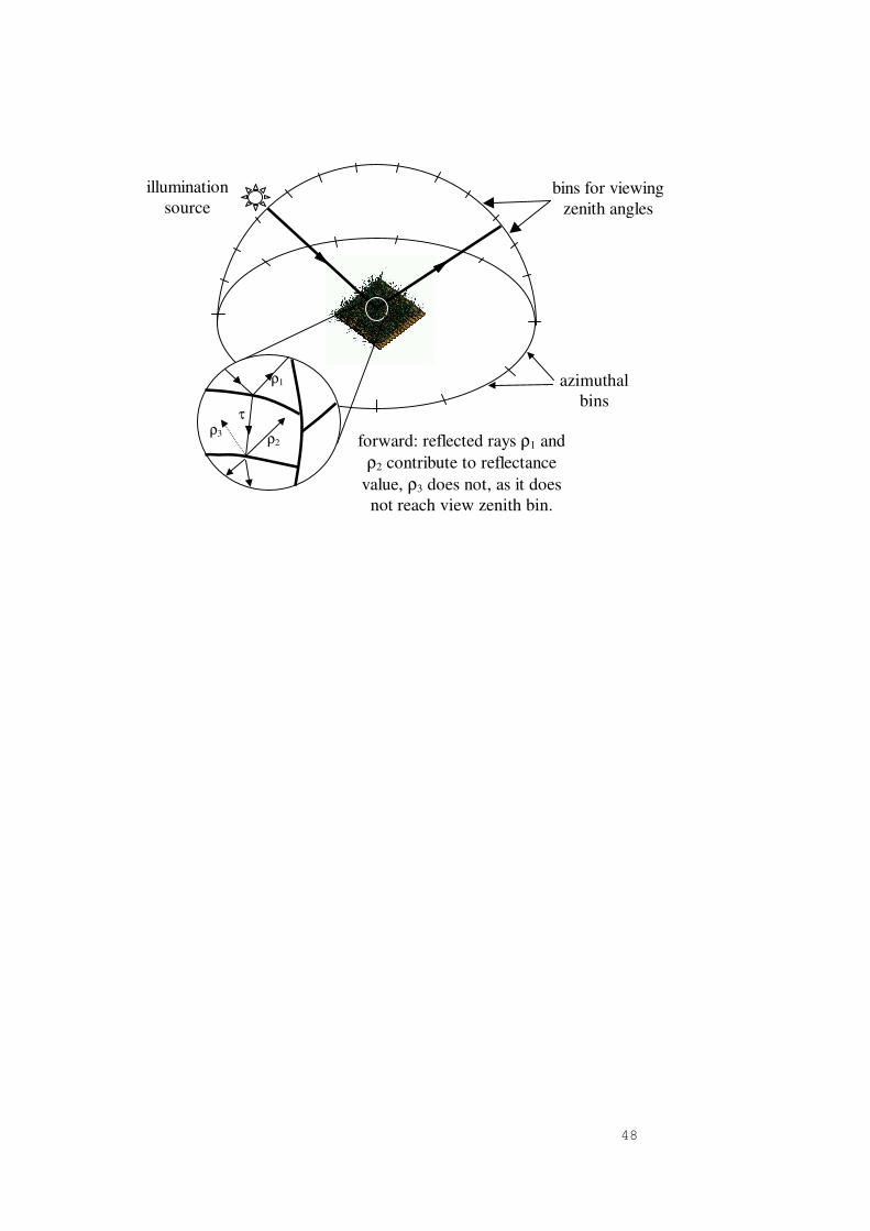
48
bins for viewingzenith angles
illuminationsource
τ
ρ1
ρ2ρ3 forward: reflected rays ρ1 and
ρ2 contribute to reflectancevalue, ρ3 does not, as it doesnot reach view zenith bin.
azimuthalbins

49
τ
ρ1
ρ2
illuminationsource
reverse: rays reflected andtransmitted through leaves;diffuse sampling rays, andrays propagating towards
source.
imagingplane
focal region ofimaging plane
(not necessarily apoint)
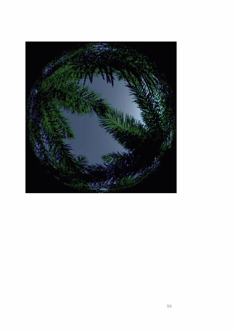
50
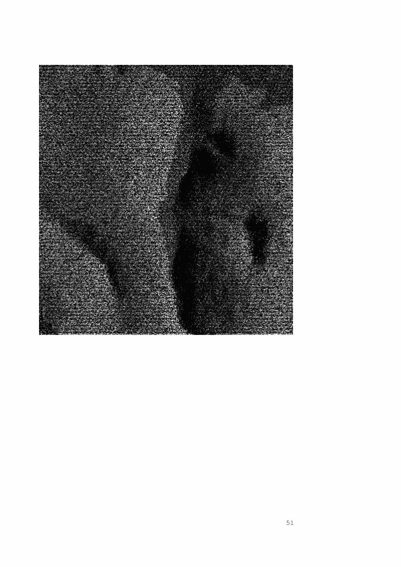
51

52
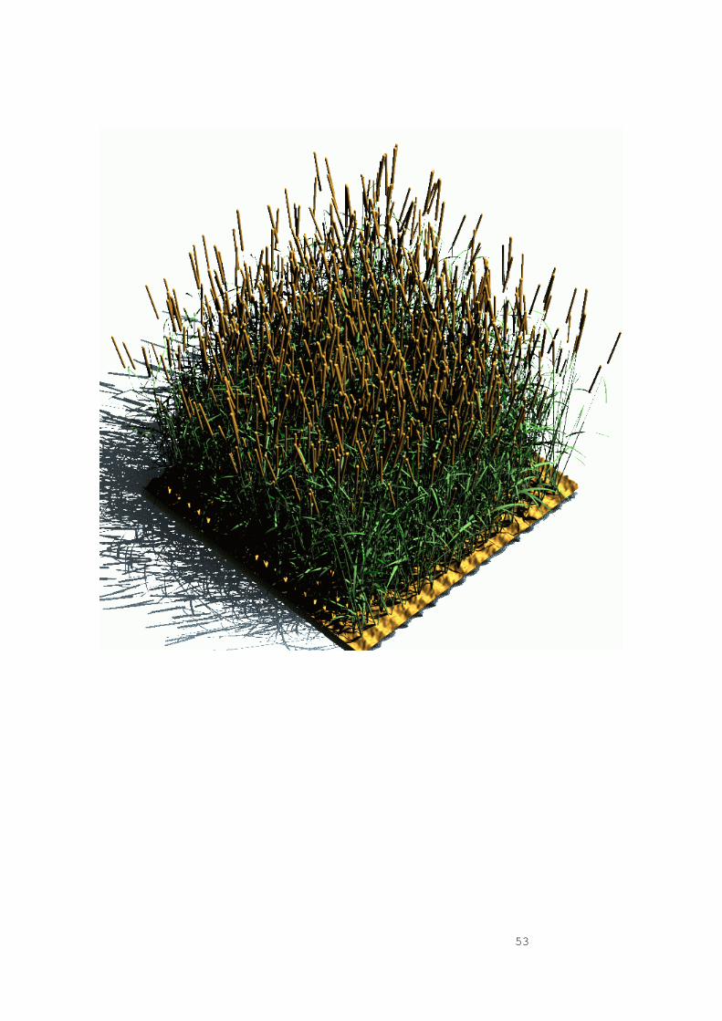
53
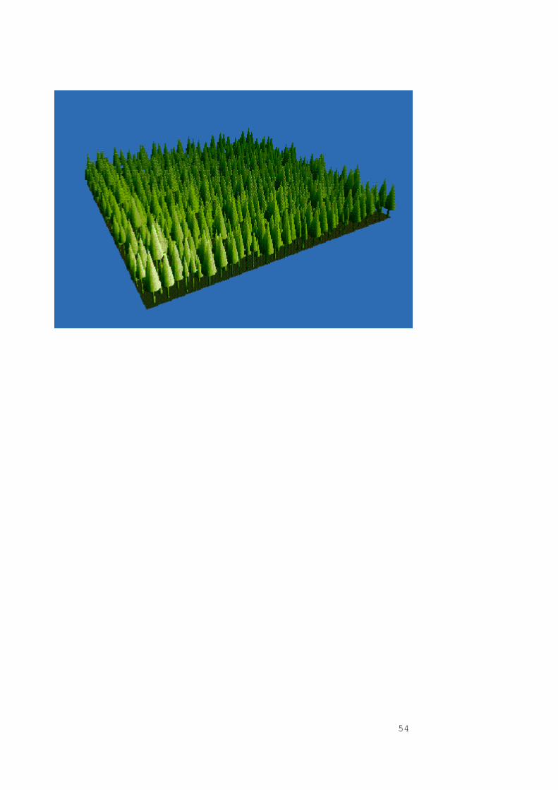
54


![Concepts and theory: Spectral reflectance, canopy ... · •Link physiology to a predicted Ideotype. ... used to estimate phenology, pests and diseases PI [R 415-R 435]/[R 415 +R](https://img.pdfslide.net/doc/110x75/5f1ac5fc02814456ea34dd26/concepts-and-theory-spectral-reflectance-canopy-alink-physiology-to-a-predicted.jpg)