Monte Carlo Simulation and Resampling - The University …carsey/teaching/ICPSR-2011/Sim Slides 2 Handout.pdf · Resampling methods share many similarities to Monte Carlo simulations

Monte Carlo Simulation and Resampling

Tom Carsey (Instructor)

Jeff Harden (TA)

ICPSR Summer Course

Summer, 2011

— Monte Carlo Simulation and Resampling 1/68

Resampling

Resampling methods share many similarities to Monte Carlo

simulations – in fact, some refer to resampling methods as a

type of Monte Carlo simulation.

Resampling methods use a computer to generate a large

number of simulated samples.

Patterns in these samples are then summarized and analyzed.

However, in resampling methods, the simulated samples are

drawn from the existing sample of data you have in your

hands and NOT from a theoretically defined (researcher

defined) DGP.

Thus, in resampling methods, the researcher DOES NOT

know or control the DGP, but the goal of learning about the

DGP remains.


Resampling Principles

Begin with the assumption that there is some population

DGP that remains unobserved.

That DGP produced the one sample of data you have in your

hands.

Now, draw a new “sample” of data that consists of a

different mix of the cases in your original sample. Repeat

that many times so you have a lot of new simulated

“samples.”

The fundamental assumption is that all information about

the DGP contained in the original sample of data is also

contained in the distribution of these simulated samples.

If so, then resampling from the one sample you have is

equivalent to generating completely new random samples

from the population DGP.


Resampling Principles (2)

Another way to think about this is that if the sample of data

you have in your hands is a reasonable representation of the

population, then the distribution of parameter estimates

produced from running a model on a series of resampled data

sets will provide a good approximation of the distribution of

that statistics in the population.

Resampling methods can be parametric or non-parametric.

In either type, but especially in the non-parametric case, yet

another way to justify resampling methods according to

Mooney (1993) is that sometimes it is, “· · · better to draw

conclusions about the characteristics of a population strictly

from teh sample at hand, rather than by making perhaps

unrealistic assumptions about that population (p. 1).”


Common Resampling Techniques

Bootstrap

Jackknife

Permutation/randomization tests

Posterior sampling

Cross-validation


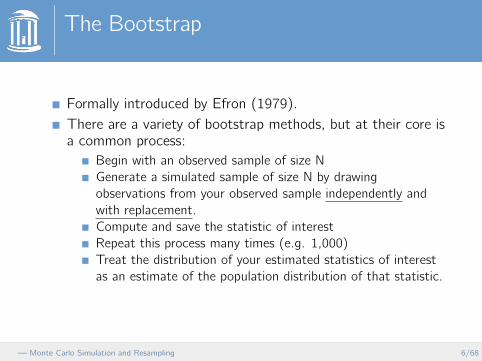
The Bootstrap

Formally introduced by Efron (1979).

There are a variety of bootstrap methods, but at their core isa common process:

Begin with an observed sample of size N

Generate a simulated sample of size N by drawing

observations from your observed sample independently and

with replacement.

Compute and save the statistic of interest

Repeat this process many times (e.g. 1,000)

Treat the distribution of your estimated statistics of interest

as an estimate of the population distribution of that statistic.


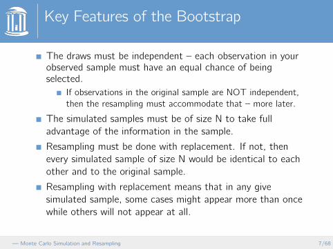
Key Features of the Bootstrap

The draws must be independent – each observation in yourobserved sample must have an equal chance of beingselected.

If observations in the original sample are NOT independent,

then the resampling must accommodate that – more later.

The simulated samples must be of size N to take full

advantage of the information in the sample.

Resampling must be done with replacement. If not, then

every simulated sample of size N would be identical to each

other and to the original sample.

Resampling with replacement means that in any give

simulated sample, some cases might appear more than once

while others will not appear at all.


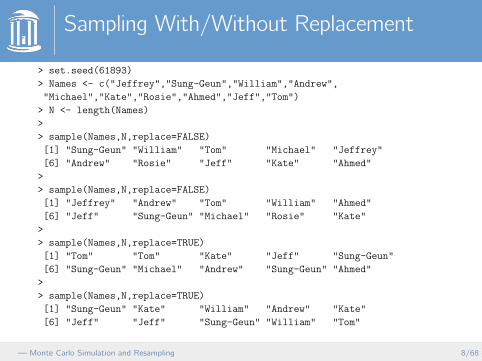
Sampling With/Without Replacement

¿ set.seed(61893)

¿ Names ¡- c(”Jeffrey”,”Sung-Geun”,”William”,”Andrew”,

”Michael”,”Kate”,”Rosie”,”Ahmed”,”Jeff”,”Tom”)

¿ N ¡- length(Names)

¿

¿ sample(Names,N,replace=FALSE)

[1] ”Sung-Geun” ”William” ”Tom” ”Michael” ”Jeffrey”

[6] ”Andrew” ”Rosie” ”Jeff” ”Kate” ”Ahmed”

¿

¿ sample(Names,N,replace=FALSE)

[1] ”Jeffrey” ”Andrew” ”Tom” ”William” ”Ahmed”

[6] ”Jeff” ”Sung-Geun” ”Michael” ”Rosie” ”Kate”

¿

¿ sample(Names,N,replace=TRUE)

[1] ”Tom” ”Tom” ”Kate” ”Jeff” ”Sung-Geun”

[6] ”Sung-Geun” ”Michael” ”Andrew” ”Sung-Geun” ”Ahmed”

¿

¿ sample(Names,N,replace=TRUE)

[1] ”Sung-Geun” ”Kate” ”William” ”Andrew” ”Kate”

[6] ”Jeff” ”Jeff” ”Sung-Geun” ”William” ”Tom”


What to Resample?

In the single variable case, you must resample from the data

itself.

However, in something like OLS, you have a choice.

Remember the “X ’s fixed in repeated samples” assumption?

So, you can resample from the data, thus getting a new mix

of X ’s and Y each time for your simulations.

Or you can leave the X ’s fixed, resample from the residuals of

the model, and use those to generate simulated samples of Y

to regress on the same fixed X ’s every time.

As before, it depends on the validity of the “fixed in repeated

samples” assumption, but also it is unlikely to matter in

practice.

Most folks resample from the data.


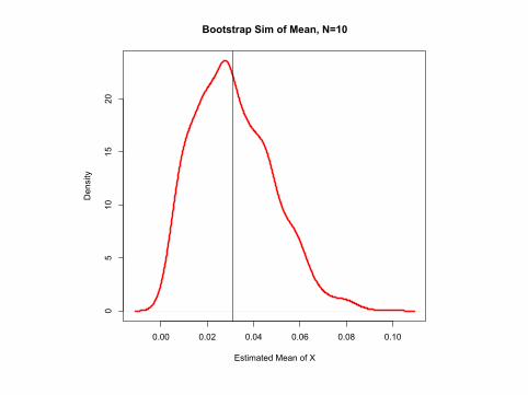
Simple Example

Let’s suppose I draw a sample of 10 folks and compute a

mean.

I could make a distributional assumption about that mean,

compute a standard error, and treat that as my best guess of

the population mean and its variance.

Or In can draw lots of resamples, compute a mean for each

one of them, and then plot that distribution


0.00 0.02 0.04 0.06 0.08 0.10

05

1015

20

Bootstrap Sim of Mean, N=10

Estimated Mean of X

Density

What Did We Learn?

The distribution of simulated sample means is close to

centered on our original sample estimate.

But the distribution is not normal, and not even symmetric.

A Bootstrap standard error would probably be better to use

than an analytic one that assumed a normal distribution.

So, how do we compute a Bootstrap standard error – and

more importantly, a Bootstrap confidence interval?

There are multiple ways


Standard Normal Bootstrap CI

This is the simplest method, mirrors the fully analytic

method of computing confidene intervals, and is parametric.

It is parametric because it assumes that the statistic of

interest is distributed normally.

You generate a large simulated sample of the parameter of

interest (e.g. a mean, a regression coefficient, etc.)

Since the SE of a parameter is defined as the standard

deviation of that parameter in multiple samples, you

compute a simulated SE as just the the standard deviation of

your simulated parameters.

A 95% CI is just your original sample parameter estimate

plus/minus 1.96 times your estimated SE.


Standard Normal Bootstrap CI (2)

The advantage is its simplicity.

The disadvantage is that it makes a distributional assumption

that may not be appropriate. If normality is a good

assumption, the analytic calculation may be appropriate.

This also implicitly assumes that your estimate of the

parameter of interest is unbiased.


Percentile Bootstrap CI

The Percentile version of the Bootstrap CI is noparametric.

This approach uses the large number of simulated

parameters of interest (e.g. means, medians, slope

coefficients) and orders them from smallest to largest.

A 95% CI is then computed by just identifying the lower CI as

the 2.5th percentile and the upper CI as the 97.5th percentile.

This leaves 95% of the simulated parameter estimates within

this range while dividing the remaining 5% of the simulated

values equally into the upper and lower tails.


Percentile Bootstrap CI (2)

The advantage of this method is it does not make any

distributional assumption – it does not even require the

distribution (or the CI) to be symmetric.

Of course, if a distributional assumption is appropriate and

you don’t use it, this approach uses less information.

In addition, this method has been shown to be less accurate

than it could be.

Still, this is the most common way to compute a Bootstrap

CI.

Side Note: This approach parallels what Bayesians do when

the compute what they call “Credible Intervals.”


Other Bootstrap CI Methods

The Basic Bootstrap CI: The simulated parameters are

adjusted by subtracting out the observed statistic, and then

the percentile method is applied.

The Bootstrap t CI: for each simulation you compute the

sample t statistic each time. Select the 2.5th and 97.5th

percentile t-scores. Use those to multiply by the simulated

SE (instead of ± 1.96).

The BCa Bootstrap CI: This method modifies the percentile

CI to correct for bias and for skewness. Simulation works

suggests better performance than the unadjusted percentile

CI.

Which to use? How to compute them?


Which CI Method to Use?

All five are available in the boot package in R by first

computing the simulated parameters and then using the

boot.ci() function. See the Lab.

The first two are pretty simple to program yourself.

They all converge toward toward the true populationdistribution of the parameter in question as:

the original sample size increases toward infinity

the number of resamples you draw increases toward infinity (If

the original sample is “large enough”)

Rules of Thumb: Replications of 1,000, sample size of 30-50

is no problem, but smaller can work if the sample is not too

“odd.”


Does this Always Work?

To some, the bootstrap seems like magic.

However, it is still fundamentally dependent on the quality of

the original sample you have in your hands.

If the original sample is not representative of the population,

the simulated distribution of any statistics computed from

that sample will also probably not accurately reflect the

population. (Small samples, biased samples, or bad luck)

Also, the bootstrap simulated distribution of a sample

statistic is necessarily discrete, whereas often the underlying

population PDF is continuous. They converge as sample size

increases, but the simulated distribution remains discrete.

Nothing is perfect!


Bootstrapping Complex Data

Resampling one observation at a time with replacement

assumes the data points in your observed sample are

independent. If they are not, the simple bootstrap will not

work.

Fortunately the bootstrap can be adjusted to accommodate

the dependency structure in the original sample.

If the data is clustered (spatially correlated, multi-level, etc.)

the solution is to resample clusters of observations one at a

time with replacement rather than individual observations.

If the data is time-serial dependent, this is harder because

any sub-set you select still “breaks” the dependency in the

sample, but methods are being developed.


When Does it Not Work Well?

Data with serial correlation in the residual (as noted in the

last slide).

Models with heteroskedasticity (other than unit-specific a la

clustered data) when the form of the heteroskedasticity is

unknown. One approach here is to sample pairs (on Y and

X) rather than leaving X fixed in repeated samples.

Simultaneous equation models (because you have to

bootstrap all of the endogenous variables in the model).


An Example

Londregan and Snyder (1994) compare the preferences of

legislative committees with the entire legislative chamber to

test if committees are preference outliers.

Competing theories:

Committees will be preference outliers due to self-selection

and candidate-centered incentive to win re-election.

Committees will NOT be preference outliers because the floor

assigns members to develop expertise for the floor to follow.

Empirical work is mixed – What are the problems?

Ideology scores are measured with error, but that error is

ignored.

Too many use analytic tests on two-sample differences of

means when they should use non-parametric tests (e.g.

bootstraps) on differences of medians.


Londregan and Snyder (cont.)

Two-sample tests fail when there are more than two groups

and some people are part of more than one group.

Two-sample tests treat all heterogeneity on a committee as

sampling error.

Theory is about the median voter, but sample means tests

do not fit that theory.

Between measurement error issues and concerns about the

statistical properties of medians, the resampled among

legislators to estimate committee and floor medians, and

then how far apart they’d have to be to be considered

“significantly” different.

Results


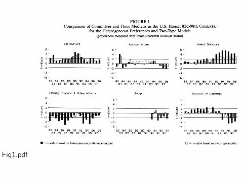
and S Fig1.pdf

One More Example

Benoit, Laver, and Mikhaylov (2009) analyze texts of the

Comparative Manifesto Project (CMP), which uses party

manifestos to measure ideological locations.

Current methods fail to consider measurement error in these

types of measures.

Use bootstraps to estimate this variability so it can be

accounted for in subsequent regression models.

The CMP data is extremely influential.


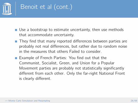
Benoit et al (cont.)

Use a bootstrap to estimate uncertainty, then use methods

that accommodate uncertainty.

They find that many reported differences between parties are

probably not real differences, but rather due to random noise

in the measures that others Failed to consider.

Example of French Parties: You find out that the

Communist, Socialist, Green, and Union for a Popular

Movement parties are probably not statistically significantly

different from each other. Only the far-right National Front

is clearly different.


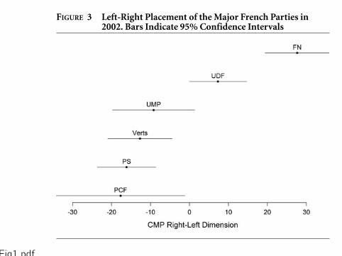
Fig1.pdf

TREATING WORDS AS DATA WITH ERROR 505

to the next is statistically significant. These results shouldbe of considerable interest to all third-party researcherswho use the CMP data to generate a time series of partypositions. They show that observed policy “changes” arestatistically significant in only 38% of relevant cases. Wedo not of course conclude from this that CMP estimatesare invalid. We do conclude that many policy “changes”hitherto used to justify the content validity of CMP es-timates are not statistically significant and may be noise.More generally, we argue that, if valid statistical (andhence logical) inferences are to be drawn from “changes”over time in party policy positions estimated from CMPdata, it is essential that these inferences are based on validmeasures of uncertainty in CMP estimates, which havenot until now been available.

While one of the CMP’s biggest attractions is un-doubtedly the time-series data it appears to offer, anothercommon CMP application involves comparing differentparties at the same point in time. Considering a staticspatial model of party competition, realized by estimat-ing positions of actual political parties at some time point,many model implications depend on differences in pol-icy positions of different parties. It is crucial, therefore,when estimating a cross-section of party policy positions,to know whether estimated positions of different partiesdo indeed differ from each other in a statistical sense.Figure 3 illustrates this problem, showing estimates ofFrench party positions in 2002, on the CMP left-right

FIGURE 3 Left-Right Placement of the Major French Parties in2002. Bars Indicate 95% Confidence Intervals

scale. Taking into account the uncertainty of these es-timates, four quite different parties—the Communists,Socialists, Greens, and Union for a Popular Movement(UMP)—have statistically indistinguishable estimatedpositions, even though the CMP point estimates seemto indicate differences. Only the far-right National Fronthad an estimated left-right position that clearly distin-guishes it from other parties. On the basis of these esti-mates we simply cannot say, notwithstanding CMP pointestimates, whether the Greens (Verts) were to the left orthe right of the Socialists (PS) in 2002. The role of uncer-tainty in cross-sectional comparisons will differ accordingto context, but the French case demonstrates—for a ma-jor European multiparty democracy—that inferences ofdifference from CMP point estimates can be ill informedwithout considering measurement error.

Correcting Estimates in Linear Models

When covariates measured with error are used in lin-ear regression models, the result is bias and inefficiencywhen estimating coefficients on error-laden variables(Hausman 2001, 58). These coefficients are typically ex-pected to suffer from “attenuation bias,” meaning they arelikely to be biased towards zero, underestimating the effectof relevant variables. This conclusion must, however, bequalified, since it depends on the relationship between the

The Jackknife

The Jackknife emerged before the bootstrap.

It’s primary use has been to compute standard error and

confidence intervals just like the bootstrap.

It is a resampling method, but it is based on drawing n

resamples each of size n-1 because each time you drop out a

different observation.

The notion is that each sub-sample provides an estimate of

the parameter of interest on a sample that can easily be

viewed as a random sample from the population (if the

original sample was) since it only drops won case at a time.

NOTE: You can leave out groups rather than individual

observations if the sampling/data structure is complex (e.g.

clustered data).


Jackknife (2)

The jackknife is less general than the bootstrap, and thus,

used less frequently.

It does not perform well if the statistic under consideration

does not change “smoothly” across simulated samples.

It does not perform well in small samples because you don’t

end up generating many resamples.

However, it is good at detecting outliers/influential cases.

Those sub-sample estimates that differ most from the rest

indicate those cases that has the most influence on those

estimates in the original full sample analysis.


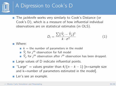
A Digression to Cook’s D

The jackknife works very similarly to Cook’s Distance (or

Cook’s D), which is a measure of how influential individual

observations are on statistical estimates (in OLS).

Di =

∑(Yj − Yji)2

k · σ2 (1)

Where:

k = the number of parameters in the model

Yj for j th observation for full model

Yji for j th observation after i th observation has been dropped.

Large values of D indicate influential points.

“Large” = values greater than 4/(n − k − 1) [n=sample size

and k=number of parameters estimated in the model].

Ler’s see an example.


30000 35000 40000 45000 50000 55000

810

1214

1618

20

Plot of Poverty and Per Capita Income Using State Postal Codes

Per Capita Income

Per

cent

in P

over

ty

AL

AK

AZ

AR

CA

CO

CT

DE

DC

FL

GA

HI

IDIL

IN

IA

KS

KY

LA

ME

MD

MA

MI

MN

MS

MOMT

NE

NV

NH

NJ

NM

NY

NC

ND

OH

OK

OR

PA

RI

SC

SD

TN

TX

UTVT

VA

WA

WV

WI

WY

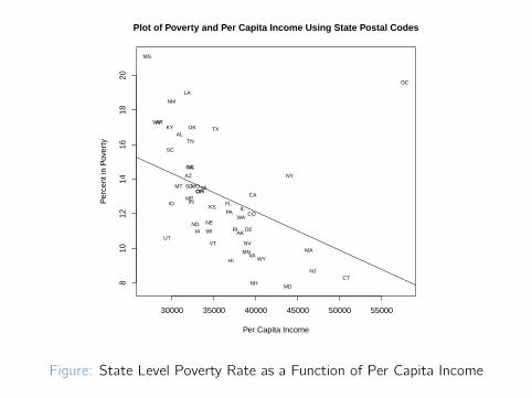
Figure: State Level Poverty Rate as a Function of Per Capita Income

01

23

4

Looking for Outliers

Coo

k's

Dis

tanc

e

1 4 7 10 14 18 22 26 30 34 38 42 46 50

ALAKAZARCACOCTDE

DC

FLGAHIIDILINIAKSKYLAMEMDMAMIMNMS

MOMTNENVNHNJNMNYNCNDOHOKORPARISCSDTNTXUTVTVAWAWVWIWY

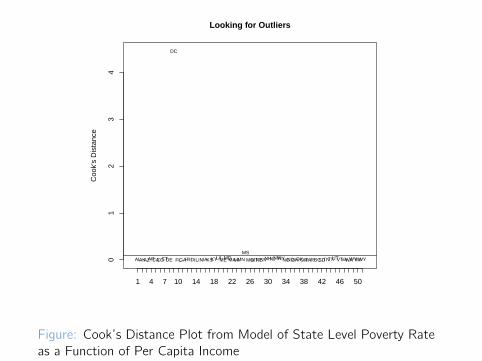
Figure: Cook’s Distance Plot from Model of State Level Poverty Rate

as a Function of Per Capita Income

Jackknife-after-Bootstrap

Rizzo (2008, pp. 195-6) suggests combining the bootstrap

and jackknife proceedures.

First, you run the bootstrap to generate your bootstrap

estimates of the parameter of interest.

Then you run a jackkife by dropping all bootstrap samples

that include the i th observation, then summarizing across

these jackknifed samples.

The procedure is available in the boot package in R .


Permutation/Randomization

Just another form of resampling, but in this case it is done

without replacement.

They have been around since Fisher introduced them in the

1930’s.

Often used to conduct hypothesis testing where the Null is

zero.

Rather than assume a distribution for the Null hypothesis, we

simulate what it would be by randomly reconfiguring our

sample lots of times (e.g. 1,000) in a way that “breaks” the

relationship in our sample data.

The question then is how often do these permutations or

randomly reshuffled data sets produce a relationship as large

or larger than the one we saw in our original sample?


Running a Permutation Experiment

Suppose we are testing the difference in means between Men

and Women on some variable.

If we have NM Men and NW Women, such that

N = NM + NW , then the total number of possible

permutations where the first group equals the number of

men and the total sample size stays the same is(NM+NW )!NM !NW !

Suppose we have a sample of 14 Men and 12 Women. If so

then we have(14+12)!14!12! = 9, 657, 700 possible permutations.

Thus, in most settings, we randomly generate some of the

possible permutations and call it good.


Additional Considerations

Randomization tests do assume exchangeability. If the Null

of no effect is true, the observed outcomes across individuals

should be similar no matter what the level of the treatment

(X ) variable is.

This is a weaker assumption than iid.

If we do examine all possible permutations, that is often

called a permutation test, or an exact test.

If we just simulate a large number, it’s called a

randomization test.

What do we reshuffle? Most reshuffle the treatment.


A Simple Example

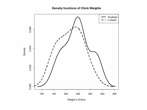
I have data on the weight of chicks and what they were fed.

The samples are small, and the distributions unknown.

Still, I want to know if their weights differ based on what

they were fed.

In a parametric world, I’d do a two-sample difference of

means t-test

But, that is only appropriate if the distributional assumption

holds.


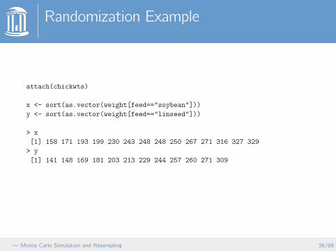
Randomization Example

attach(chickwts)

x ¡- sort(as.vector(weight[feed==”soybean”]))

y ¡- sort(as.vector(weight[feed==”linseed”]))

¿ x

[1] 158 171 193 199 230 243 248 248 250 267 271 316 327 329

¿ y

[1] 141 148 169 181 203 213 229 244 257 260 271 309


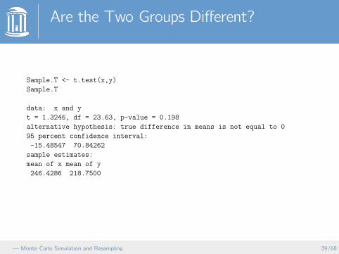
Are the Two Groups Different?

Sample.T ¡- t.test(x,y)

Sample.T

data: x and y

t = 1.3246, df = 23.63, p-value = 0.198

alternative hypothesis: true difference in means is not equal to 0

95 percent confidence interval:

-15.48547 70.84262

sample estimates:

mean of x mean of y

246.4286 218.7500


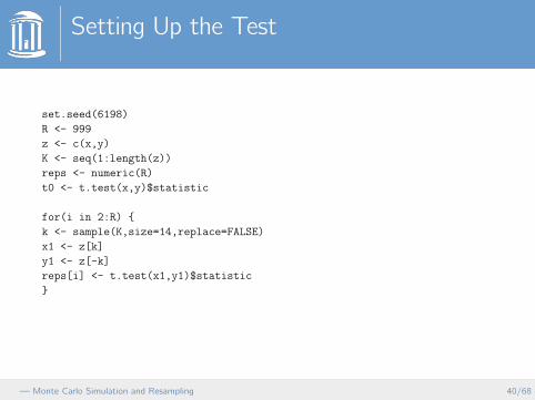
Setting Up the Test

set.seed(6198)

R ¡- 999

z ¡- c(x,y)

K ¡- seq(1:length(z))

reps ¡- numeric(R)

t0 ¡- t.test(x,y)$statistic

for(i in 2:R) –

k ¡- sample(K,size=14,replace=FALSE)

x1 ¡- z[k]

y1 ¡- z[-k]

reps[i] ¡- t.test(x1,y1)$statistic

˝


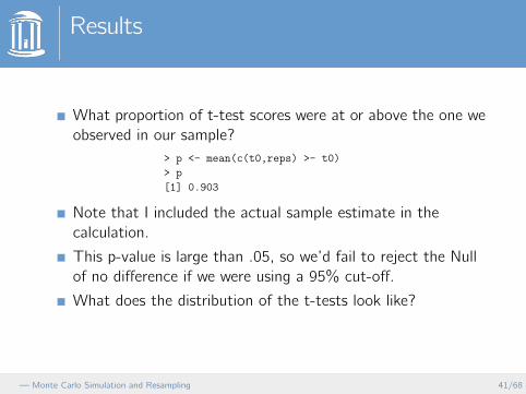
Results

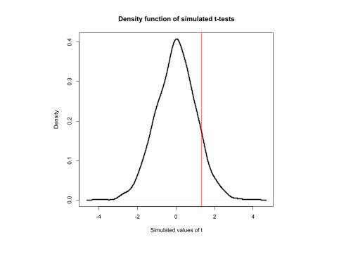
What proportion of t-test scores were at or above the one we

observed in our sample?

¿ p ¡- mean(c(t0,reps) ¿- t0)

¿ p

[1] 0.903

Note that I included the actual sample estimate in the

calculation.

This p-value is large than .05, so we’d fail to reject the Null

of no difference if we were using a 95% cut-off.

What does the distribution of the t-tests look like?


-4 -2 0 2 4

0.0

0.1

0.2

0.3

0.4

Density function of simulated t-tests

Simulated values of t

Density

What Did We Learn?

It does not look like the means of these two groups differ

significantly (at least at the .05 level of significance).

We can compare any aspect of these two samples the same

way – compute the statistic every time for a thousand

replications and then look at their distribution.

In fact, there are tests to evaluate whether the two

distributions are statistically significantly different or not.


100 150 200 250 300 350 400

0.000

0.002

0.004

0.006

Density functions of Chick Weights

Weight in Grams

Density

SoybeanLinseed

Example: Legislative Networks

Legislators form networks of cooperation, in this case, via

co-sponsorship of bills.

Those connections are intentional actions that signal

relationships.

Does party structure those relationships? We can measure

network modularity due to partisanship.

Modularity measures how well a division separates a network

into distinct groups by measuring the number of ties within a

group versus the number of ties between groups.

But what is the distribution of modularity? Let’s estimate it

rather than assume it.


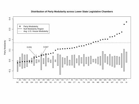
Kirkland (2011)

Modularity is bounded between -1 and 1, but no known

distribution.

Kirkland simulates that distribution by randomly partitioning

the network 25,000 times (basically randomly assigning

legislators to two “teams”)

The population PDF is then estimated by the 25,000

modularity statistics computed on randomly partitioned

networks.

Use a percentile method to compute 95% confidence

interval, and compare the observed modularity in a chamber

to this null distribution.

Party matters


●● ● ● ● ● ●

● ●●

● ●● ●

● ●

●● ● ● ● ● ● ● ● ●

● ● ●●

● ●● ● ●

● ● ● ●

● ●●

●●

●

●

●

−0.

10.

00.

10.

20.

30.

4Distribution of Party Modularity across Lower State Legislative Chambers

Par

ty M

odul

arity

● Party ModularityNull Modularity RegionAvg. U.S. House Modularity

NC IN DE OH CO WY ND NJ KY UT FL MN CT AL TN OR PA ME NH MI MT AZ CA IAAK MS HI OK SD AR MD LA WV NV VT RI NY SC TX GA WI NM WA MA KS MO VA

0.031 0.047

Comparing Methods

Bootstrap is the most flexible and most powerful. It can be

extended to any statistical or calculation you might make

using sample data.

Bootstraping does NOT make the exchangeability

assumption that randomization tests make.

Jackknife is limited by sample size

Permutation/Randomization methods break all relationships

in data – don’t let you produce a covariance matrix.[but what

if we reshuffled just on Y ?]

I think Bootstrap confidence intervals, etc. will be standard

in empirical social science in 5-10 years.


Posterior Simulation (PS)

Definition: a simulation-based approach to understanding

patterns in our data

Of course, we want to go beyond our data to draw inference

about the population from which it came.

A straightforward way to go beyond simple tables ofregression coefficients

Calculate “quantities of interest” (QI)

Account for uncertainty

Uses Bayesian principles, but does not require Bayesian

models

Example: CLARIFY in Stata (King, Tomz, and Wittenberg

2000)



Key assumption: coefficients/SEs we estimate are drawnfrom a probability distribution that describes the largerpopulation

Coefficients define the mean, SEs define the variance

With large enough sample size, according to the central limittheorem this distribution is multivariate normal

Instead of a bell curve, imagine a jello mold that can take on

different colors, flavors, and textures

The goal of PS: make random draws from this distribution to

simulate many “hypothetical values” of the coefficients

Instead of drawing one single number, as with rnorm(), we

draw a vector of numbers (one for each coefficient)



The next step: choose a QI

Expected value, predicted probability, odds ratio, first

difference, change in hazard rate, etc. . .

Set a key variable in the model to a theoretically interesting

value and the rest to their means or modes

Calculate that QI with each set of simulated coefficients

Set the variable to a new value

Calculate that QI with each set of simulated coefficients

Repeat as appropriate



At every value of the variable, we now have many

calculations of the QI

Final step: efficiently summarize the distribution of the

computed QI at each value of our variable

Most common: point estimate and confidence intervals

Can represent this in a table or graph (we will do a graph

example)


Advantages of PS

Provides more information than a just a table of regression

output

Accounts for uncertainty in the QI

Flexible to many different types of models, QIs, and variable

specifications

After doing it once, easy to use

Can be much easier than working with analytic solutions


Limitations of PS

Relies on CLT to justify asymptotic normality

Fully Bayesian model using MCMC could produce exact

finite-sample distribution

Bootstrapping would require no distributional assumption

Computational intensity

Large models can produce lots of uncertainty around quantity

of interest


Motivation for Cross-Validation (CV)

A key component of scientific research is the independent

assessment and testing of our theories.

Lave and March (1979) model of theory building:

Observe something in the world

Speculate about why it appears the way it does (develop a

theory)

If your theory were true, what else would you expect to

observe?

Testing a your theory involves exploring that “what else.”

The “what else” might involve other dependent variables,

but it might also involve the same dependent variable in an

independently drawn sample of data

The key is: Data that helps you build your theory cannot

also be used as an independent test of theory


Motivation for CV (2)

Using the same data to build and “test” a theory leads to

over-fitting a statistical model to your sample.

Such over fitting to the sample captures aspects of the true

population DGP you care about . . .

But, it also captures elements that are peculiar to your

particular sample that are NOT reflective of the true DGP.

Thus, over-fitting a model to your sample actually leads to

worse/less accurate inference about the population from

which it came.


Motivation for CV (3)

How can you avoid using the same data to build and then

“test” your theory?

Develop your theory, specify your model, etc. before looking

at your data, then run the statistical analysis you planned

one time and write it up.

Use the data you have to build your model, then collect fresh

data to test it.

Divide the data you have so you use some of it to build your

model and some of it to independently test it.

This last option is cross-validation


Cross-Validation (CV)

Definition: a method for assessing a statistical model on a

data set that is independent of the data set used to fit the

model

Often used in disciplines like computer science that focus on

predictive models

Goal: guard against “Type III” errors—the testing of

hypotheses suggested by the data (i.e., overfitting)

Many different types based on different ways of constructing

the independent data

Many different fit statistics can be calculated in a CV routine


CV Example: The Netflix Prize

Key component of Netflix: recommend the right movies to

the right people

Main data source: customers’ own ratings of movies they

have seen

2009: $1 million prize for beating Netflix’s current prediction

system

Netflix provided 100 million ratings from 480,000 users of

18,000 movies

Teams developed models predicting ratings in these data

Submissions were then evaluated on 2.8 million ratings not

included in the data given to teams


CV Example: The Netflix Prize

The winning team beat Netflix’s own system by 10% as

judged by mean squared error

Why was it important to set aside the 2.8 million ratings for

model evaluation?

If the evaluation was done on the 100 million, teams couldhave “gamed the system”

Find the odd quirks of that particular sample that came about

due to random sampling

Overfit the model to account for these odd quirks

This would make the model look really good on this one

sample, but it wouldn’t be generalizable to other samples

For more information: http://www.netflixprize.com/

assets/GrandPrize2009˙BPC˙BellKor.pdf


http://www.netflixprize.com/assets/GrandPrize2009_BPC_BellKor.pdf

http://www.netflixprize.com/assets/GrandPrize2009_BPC_BellKor.pdf

CV Example: Predicting Divorce

Psychologist featured in Malcolm Gladwell’s book Blink

Research on whether a couple will get divorced based on

watching them argue for 15 minutes

Videotaped 57 couples, coded several variables

Claims 80-90% accuracy (amazing!)

But there are problems. . .


CV Example: Predicting Divorce

“Predictive formula” developed with knowledge of the

couples’ marriage outcomes

Then the formula was applied to those same couples

Are we still amazed that he got 80% right?

A better test: get a new sample of couples and apply the

formula to them

For more information:

http://www.slate.com/id/2246732/


http://www.slate.com/id/2246732/

Stagflation

The 1970s saw a period thought impossible in a modern

economy – high unemployment AND high inflation.

Most statistical models of the economy at the time fail to

predict this. Why?

Forecasters used massively large models that includedhundreds of variables. This resulted in forecasting failure doto:

Massive uncertainty in a model that is estimating

hundreds/thousands of parameters.

Over-fitting the sample data.


CV Examples

These examples show us the importance of out-of-sample

prediction

There are always oddities in a particular sample

We don’t want to fit our models to those oddities

CV only rewards models for picking up general patterns that

appear across samples

The problem: where do we get a new sample?


General CV Steps

1 Randomly partition the available data into a training set and

a testing set

2 Fit the model on the training set

3 Take the parameter estimates from that model, use them to

calculate a measure of fit on the testing set

4 Can repeat steps 1–3 several times, average to reduce

variability


Two Types of CV

Split-sample CV:

Partition into 50% training, 50% testing (could also do

75/25, 80/20, etc. . . )

Usually want to maximize size of training set

Particularly common in time series analysis where the testing

data is generally the most recent years for which data is

available.

Leave-one-out CV:

Iterative method with number of iterations = sample size

Each observation becomes the training set one time

Note the parallel to the Jackknife and Cook’s D.


Leave-One-Out CV

1 Delete observation #1 from the data

2 Fit the model on observations #2–n

3 Apply the coefficients from step #2 to observation #1,

calculate the chosen fit measure

4 Delete observation #2 from the data

5 Fit the model on observations #1 and #3–n

6 Apply the coefficients from step #5 to observation #2,

calculate the chosen fit measure

7 Repeat until all observations have been deleted once


Limitations of CV

Training and testing data must be random samples from the

same population (Why?)

Will show biggest differences from in-sample measures when

n is small (Why?)

Higher computational demand than calculating in-sample

measures

Subject to researcher’s selection of an appropriate fit statistic


Documents

Monte Carlo Simulation and Resampling - The University …carsey/teaching/ICPSR-2011/Sim Slides 2 Handout.pdf · Resampling methods share many similarities to Monte Carlo simulations