Embed Size (px)
Citation preview
AD-A245 910
NAVAL POSTGRADUATE SCHOOLMonterey, California
DTICv.-LECTE
D -THESIS
22 M
AN APPRAISAL OF COST-EFFECTIVENESS MODELS USED IN THEAIR FORCE AND NAVY AIRCRAFT ENGINE COMPONENT
IMPROVEMENT PROGRAMS
by
James D. Davis
December 1991Thesis Advisor: Alan W. McMasters
Approved for public release; distribution is unlimited
92-03538
9l) "

SECURITY CLASSIFICATION OF THIS PAGE
REPORT DOCUMENTATION PAGEla REPORT SECURITY CLASSIFICATION lb RESTRICTIVE MARKINGSUnclassified
2a SECURITY CLASSIFICATION AUTHORITY 3 DISTRIBUTION/AVAILABILITY OF REPORT
Approved for public release; distribution is unlimited.2b DECLASSIFICATION/DOWNGRADING SCHE DULE
4 PERFORMING ORGANIZATION REPORT NUMBER(S) 5 MONITORING ORGANIZATION REPORT NUMBER(S)
6a NAME OF PERFORMING ORGANIZATION 6b OFFICE SYMBOL 7a NAME OF MONITORING ORGANIZATIONNaval Postgraduate School (If applicable) Naval Postgraduate School
55
6c ADDRESS (City, State, and ZIP Code) 7b ADDRESS (City, State, and ZIP Code)Monterey, CA 93943-500) Monterey, CA 93943-5000
8a NAME OF FUNDING/SPONSORING 8 8b OFFICE SYMBOL 9 PROCUREMENT INSTRUMENT IDENTIFICATION NUMBERORGANIZATION (If apphcable)
8c ADDRESS (City, State, andZIP Code) 10 SOURCE OF FUNDING NUMBERSPrOqjdm Element No Protect No 1a$k No Work unit ACce On
Number
11 TITLE (Include Security Classification)
AN APPRAISAL OF COST EFFECTIVENESS MODELS USED IN THE AIR FORCE AND NAVY AIRCRAFT ENGINE COMPONENTIMPROVEMENT PROGRAMS
12 PERSONAL AUTHOR(S) James1). DavisUSN
13a TYPE OF REPORT 13b TIME COVERED 14 DATEOF REPORT (year, month,day) 15 PAGECOUNTMaster's Thesis From To December. 1991 9416 SUPPLEMENTARY NOTATIONThe views expressed in this thesis are those of the author and do not reflect the official policy or position of the Department of Defense or the U.S.Government.17 COSATI CODES 18 SUBJECT TERMS (continue on reverse if necessary and identify by block number)
FIELD GROUP SUBGROUP Component Improvement Program CIP)Life Cycle Costs (ICCi
19 ABSTRACT (continue on reverse if necessary and identify by block number)
This thesis examines the cost-eflettiveness models used by the Air Force and Ntvy to ass:st with the decision-making process of their ComponentImprovement Programs iCIPi. The focus is on the elements of the two models and the reasonableness ofeach model's results. A sensitivityanalysis as performed on sigificant input parameters to determine what effect errors in these parameters would have on the predicted returnon-investment IROI resullt. The author concluded that, although the models provide insight into the life cycle costs I LCC) of aircralt engines,they are extremely sesitive to errors in certain input variables and should not be relied upon for Cl P budget justification.
20 DISTRIBUTION/AVAILABILITY OF ABSTRACT 21 ABSTRACT SECURITY CLASSIFICATION
E INCiASSMEiPIiiMIlit, 13AP.i AHLPORT ta3 1,11C L'ii clussified22a NAME OF RESPONSIBLE INDIVIDUAL 22b TELEPHONE (Include Area code) 22t OFFICE SYMBOLAlan W. McMasters 408 646 2678 AS(NI(
DD FORM 1473,84 MAR 83 AIR edition may be used uniil exhausted SECURITY CLASSIFICAltOt1 Of THIS PAGEAll other editions are obsolete
Approved for public release; distribution is unlimited.
AN APPRAISAL OF COST-EFFECTIVENEESS MODELS USEDIN THE AIR FORCE AND NAVY
AIRCRAFT ENGINE COMPONENT IMPROVEMENT PROGRAMS
by
James D. DavisLieutenant, United States Navy
B.S., State University of New York, College at Oswego
Submitted in partial fulfillment
of the requirements for the degree of
MASTER OF SCIENCE IN MANAGEMENTfrom tne
NAVAL POSTGRADUATE SCHOOLDecember 1991
Author:S James D. Davis
Approved by: d&l ii- 0j Alio IAlan W. McMasters, Thesis Advsor
Kishore Sengt Ad isor
D eadV R. Whiple, Chairma;n c
Department of Administrative Scienc
ABSTRACT
This thesis examines the cost-effectiveness models used by the Air Force and Navy to assist
with the decision-making process of their Component Improvement Programs (CIP). The focus is
on the elements of the two models and the reasonableness of each model's results. A sensitivity
analysis was performed on significant input parameters to determine what effect errors in these
parameters would have on the predicted return-on-investment (ROI) results. The author concluded
that, although the models provide insight into the life-cycle costs (LCC) of aircraft engines, they are
extremely sensitive to errors in certain input variables and should not be relied upon for CIP budget
justification.
Accesion ForNTIS CRA&I
DTICiAB [U::a ,,:ou.;red _
J1stifcationEy..................
Dist ib.ition I
Availabffity Codes
Avail p:.a orDit Sp :cial
iiAl

TABLE OF CONTENTS
I. INTRODUCTION .................... 1
A. BACKGROUND ....... ................. I
B. OBJECTIVES ........... ............ .. 2
C. LIMITATIONS .......... .................. 3
D. METHODOLOGY .......... ................ 3
E. ORGANIZATION OF THE THESIS ...... ......... 4
II. BACKGROUT D ........... ................... 5
A. WHAT IS CIP .......... ................. 5
B. WHAT ARE THE OBJECTIVES OF CIP .... ........ 6
C. WHO IS RESPONSIBLE FOR CIP ..... .......... 7
D. THE AIR FORCE COMPONENT IMPROVEMENT PROGRAM . . 9
E. THE NAVY COMPONENT IMPROVEMENT PROGRAM . . . 10
III. LITERATURE REVIEW AND THEORETICAL FRAMEWORK . . 15
A. LOGISTICS ENGINEERING CONCEPTS .. ........ 15
1. Cost Effectiveness (C-E) .. ......... 15
2. Reliability ...... ................ 16
3. Reliability Prediction ... .......... . 16
4. Maintai.nability ..... ............. 17
5. Mean Time Between Maintenances (MTBM) . . . 17
6. Life Cycle Costs (LCC) .... ........ 18
iv
7. Return on Investment (ROI) .. ........ 18
8. Net Present Value (NPV) .. .......... 18
B. COST ANALYSIS MODELS .... ............. 19
C. AIRCRAFT ENGINE LIFE CYCLE COST ANALYSIS . . . 21
IV. THE AIR FORCE MODEL ...... .............. 24
A. BACKGROUND OF THE AIR FORCE MODEL ...... . 24
B, FORMAT OF CEAMOD ..... ............. . 24
C. DESCRIPTION OF INPUT PARAMETERS 1.0 THROUGH
21.0 ........ ..................... 25
D. DESCRIPTION OF INPUT PARAMETERS 22.0 THROUGH
53.0 ......... .................... 30
E. DISCUSSION OF THE RESULTS SUMMARY SECTION . . 36
F. SENSITIVITY AlRALYSIS CF SIGNIFICANT INPUT
PARAMETERS ....... ................. 40
V. THE NAVY MODEL ........ ........... ... 43
A. BACKGROUND OF THE NAv1Y MODEL .. ........ 43
B. FORMAT OF THE NAVY'S ROI MODEL .. ........ 44
C. DISCUSS::ON OF THE BASIC DATA PARAMETERS . . . 45
D. DISCUSSION OF THE EXPECTFP COST SECTIONS . . 52
E. DISCUSSION OF THE RETURN ON INVESTMENT SECTION 53
F. SENSITIVITY ANALYSIS OF SIGNIFICANT INPUT
PARAMETERS ...... ................ .. 54
G. DIFFERENCES BETWEEN THE AIR FORCE AND NAVY
MODEL ........ ..................... 57
V

VI. SUMMARY, CONCLUSIONS AND RECOMMENDATIONS ........ 60
A. Summary......................so
B. CONCLUSIONS....................61
C. Recommendations...................62
APPEXDIXA........................63
APPEXDIX B........................76
LIST OF REFERENCES....................85
DISTRIBUTION LIST.....................87
vi
I. INTRODUCTION
A. BACKGROUND
This thesis will examine whether the Air Force and Navy's
cost analysis models for the Component Improvement Program
(CIP) are accurate enough to provide sound support in the CIP
decision making process.
The Navy is facing a situation in which no new tactical
aircraft will be deployed before 2005. This factor, combined
with Congressional pressure to sustain readiness while
lowering costs, will plac- a severe strain on logistical
support for our tactical aircraft. The Navy wi.l be forced to
extend aircraft beyond their planned c-.eratioal life while,
at the same time, trying to lower operating and support costs
for these aircraft.
One method to lcwer readiness costs is through CIP. The
Componert Improvement Program is an expensive program which
calls for significant investment with the expectation of lower
ope ations and support costs. However, justifying CIP
inve .:ment from an economic standpoint requires a cost
analysis model which will accurately portray the return on
investment (ROI). This return is based on the expected
savings from reduced life-cycle costs.
1

The key question becomes: Are we able to accurately
determine the cost savings associated with CIP investment? In
order to correctly prioritize and justify Engineering Planning
Documents (EPD) and Engineering Change Proposals (ECP) for
life cycle cost improvements, a model must be developed which
reliably portrays the relevant costs and savings expected as
a consequence of the component improvement. The Air Force and
Navy currently use computer-based models which perform cost-
benef it calculations based on certain sets of inputs and
assumptions.
This thesis is concerned with the validity of the
assumptions, data inputs and formulas incorporated into these
computer-based models ard attempts to provide an objective
viewpoint concerning these issues.
B. OBJECTIVES
The primary objectives of this thesis focus on three steps
which are:
1. Conduct a literature review of logistics engineering
concepts to determine reasonable procedures for calculating
life cycle costs and ROI analysis.
2. Evaluate the Cost Analysis models used in the
decision-making process of the Air Force and Navy for the
Component Improvement Program (CIP).
3. Determine if the models in step 2 accurately reflect
life cycle costs and return on investment for aircraft engine
2
component improvements based on the information obtained in
step 1. If not, then suggest improvements which should be made
in these models.
C. LIMITATIONS
The primary limitation to this study is the relative
recent implementation of the current Navy and Air Force
models. It is extremely important to validate the
recommendations from the models with historical results.
However, because the models have only recently been developed,
there has not been sufficient time to obtain data for such a
validation.
Another serious limitation has been the inconsistencies of
information obtained from contra.ctors and cognizant military
commands. These were primarily related to the interpretations
of data inputs and assumptions. These inconsistencies appear
to also be due to the relative newness of the models.
D. METHODOLOGY
In order to objectively analyze the Air Force and Navy CIP
cost analysis models, a sound basis must be established with
regard to the reasonableness of various costing techniques.
Acceptable methods for formulating a basis of current versus
future costs need to be determined. The literature review of
applicable logistic engineering concepts and their influence
on life cycle cost models will provide that basis.
3

The Air Force and Navy CIP cost models will be then
examined in an attempt to reveal th:e reasons for the
assumptions and mathematical formulas. To accomplish this,
the author obtained the computer coding for both models.
E. ORGANIZATION OF THE THESIS
Chapter II presents a framework for u-,derstanding the
aircraft engine Component Improvement Program. The functions,
objectives and evaluation criteria for CIP are all described
in enough detail to provide the reader a basic knowledge of
the program.
Chapter III describes the results of the literature
review. As mentioned above, the intent is to establish an
adequate background for understanding the costs associated
with a system's life cycle and the effects which various
factors such as reliability and maintainability play in a cost
analysis3 model.
Chapter IV provides an evaluation of the Air Force model
to determine the reasonableness of its variables and
mathematical formulas. Chapter V provides a comparable
evaluation of the Navy model.
Chapter VI contains a summary of the thesis, conclusions
reached from the analyses, and reconendations for
improvements.
4
!I. BACKGROUND
A. WHAT IS CIP
It is common practice for aircraft gas turbine engines to
be released into operation prior to solving all of their
design inadequacies. The trade-off between Full Scale
Development (FSD)l and future component improvements is made
to ensure that an engine can enter operational service at a
reasonable cost. Deficiencies which were not identified
during the research and development (R&D) phase are corrected
through continuing investments in design improvements of the
in-service gas turbine engine. Initially these are r'Aated to
safety; later they are related to reliability and
maintainability. [Ref. 1:p. I-1
Funding for CIP in the defense budget moved from the
Aircraft Procurement Account to the Research, Development,
Testing, and Evaluation (RDT&E) Account in fiscal year 1981.
The funding transfer was directed by Congress and resulted
from a General Account:ng Office study on CIP. The study
concluded that CIP was essential, but that the efforts
primarily involved research and development. [Ref. 2:p. 23
'Full scale development refers to the phase betweenvalidation and production. During FSD, work proceeds towarddevelopment of operational capability.
5
B. WHAT ARE THE OBJECTIVES OF CIP
The basic objectives of CIP are:
- Solve as quickly as possible any safety-of-flight
problems identified to engine design inadequacies.
- Correct design inadequacies which create
unsatisfactory engine performance.
- Reduce engine Life Cycle Cost (LCC) by improving
reliability, maintainability and supportability.
[Ref. 3:p. 1]
These objectives are reached through coordination of
engineering, manufacturing, testing, quality control, and
management functions. The Component Improvement Program is
not designed to address improvement of the engine performance;
development of prototypes; or examination of additional
applications. Furthermore, CIP does not address issues which
are covered under the engine's warranty program. [Ref. 1:pp.
1-2 to 1-7]
Two of the three objectives of CIP, solving safety-of-
flight and correction of unsatisfactory engine performance,
are meant to address prevention of Class A accidents2 and
fleet-wide grounding of aircraft for serious problems. These
problems are usually discovered early in an engine's
operational life.
2Class A mishaps are accidents which cause greater than500 thousand dollars in damage, damage the aircraft beyondrepair, or cause a serious casualty (fatal/pernmanentlydisabled).
6
The third objective, improving the logistics aspects of an
aircraft engine, requires the CIP manager to consider the
entire life-cycle of the engine and determine ways to lower
operating and support costs. An improvement in the
reliability and maintainability of the engine will potentially
lower the labor and material costs associated with the
operating and support costs.
Figure 1 on the following page provides a flowchart which
outlines the evaluation process of initiating a design change.
[Ref. 4:p. 961
C. WHO IS RESPONSIBLE FOR CIP
The Department of Defense (DOD) is a key player in
aircraft engine CIP, helping to identify design inadequacies
and fund their correction. As previously mentioned, the
Military CIP program falls under RDT&E in the defense budget
with each service (Air Force, Navy, and Army) separately
managing their cognizant engines. There is a Tri-Service
Aircraft Engine Component Improvement Program which
coordinates CIP efforts on engines which are shared by two or
more of the services.
The tri-service agreement calls for selecting a lead
service to coordinate all CIP efforts on the shared engine.
The tri-service agreement also includes funding support from
Foreign Military Sales (FMS) customers and, in cases where
7
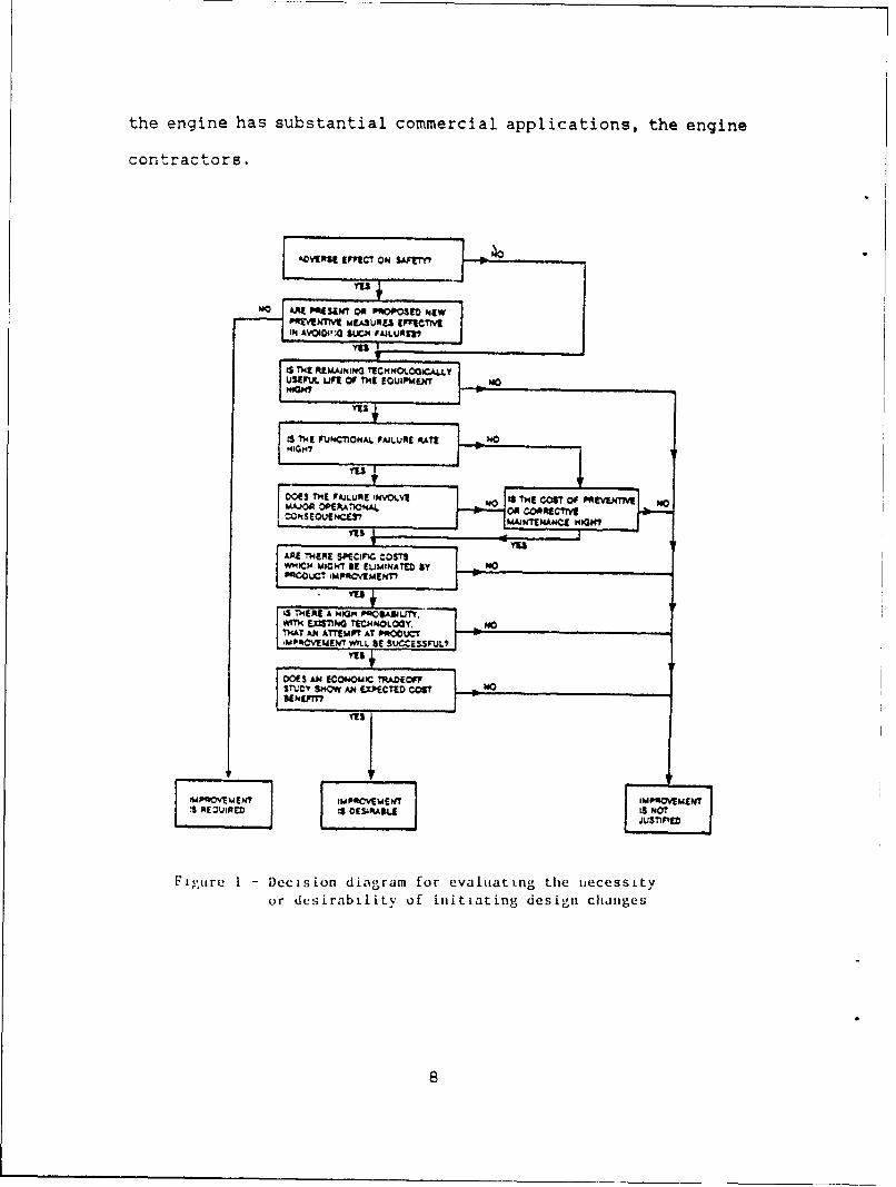
the engine has substantial commercial applications, the engine
contractCors.
fo YERS T 1AJLUN N~~ Un CS O PvpT~
No AREPSENT 0 OOj 0 EMANT mAJN1SANC tMC0147
4 L EMJIN SECC COS7U
MPNvAlM FAIL R E RATCES L 4
SIOY S THE AJVEPIECE COSTXV No___________COSTOf___________
MAOFOEL201PA 0 ORETj1ME3EOcUj SCESIRASLA SA 44OT
Y131~I
Figre1 Dciio digrm orevlutin Le ~ees~tRE TERablt ofCII intainOein Mn
W"IM IGT E LIINTE B8N
D. THE AIR FORCE COMPONENT IMPROVEMENT PROGRAM
The Air Force CIP effort is managed by the Air Force
System Command (AFSC) through the Aeronautical Systems
Division's (ASD) Directorate of Plans and Projects within the
Propulsion System Program Office. The Aeronautical Systems
Division is located at Wright-Patterson Air Force Base, Ohio.
The coordination of CIP for all Air Force engines includes
(1) the preparation, combination and submission of budget
requests for engine CIP, (2) policy review and guidance for
engine managers, (3) the coordination of CIP funds to ensure
all funds are forwarded to the appropriate organizations with
respect to the Engine Advisory Group's (EAG) recommendations,
(4) the management of all financial data on commitments,
obligations, and expenditures for CIP funds, and (5)
sponsorship of the EAG. [Ref. 5:p. 3]
The Engine Advisory Group is composed of members from
ASD's Propulsion System Program Office and members of the
Engineering Logistics and Material Management Offices. The
EAG is responsible for reviewing and prioritizing all Air
Force CIP funding. Each engine manager ranks his engine tasks
and meets with the EAG in order to develop an overall plan for
CIP funding. A cost-analysis model has been incorporated into
the Air Force prioritization process in order to compare CIP
tasks which are specifically designed to lower life cycle
costs. This model will be discussed in Chapter IV.
9
E. THE NAVY COMPONENT IMPROVEMENT PROGRAM
The Navy's CIP effort is managed by the Naval Air Systems
Command. The specific responsibilities are detailed to the
Propulsion and Power Division (AIR-536) with assistance from
the Maintenance Policy and Engineering Division (AIR-411).
The precise duties are as follows:
(1) AIR-536
(a) Plan, budget, and allocated CIP funds.
(b) Implement, execute and manage the program.
(c) Coordinate CIP with the Air Force and Army to
achieve the maximum benefits from CIP within
funding constraints.
(d) Integrate Foreign Military Sales for CIP.
(e) Justify the level of funding that is required
to incorporate modifications resulting from
approved ECPs.
(2) AIR-411
(a) Assess the logistic support impact of proposed
ECPs and make any required adjustments to the
maintenance plan. [Ref. 3:p. 4]
The Navy's evaluation procedures for CIP proposals are
designed to comply with the regulations set out in the
Competition in Contrating Act (CICA) of 1984. Each proposal
is subjected to a uniform evaluation which addresses the
following questions [Ref. 2:pp. 4-11]:
a. What is the proposed program trying to do and why?
10
b. How will the objective be accomplished?
c. What are the alternate strategies or approaches to
accomplish the objective?
d. What are the total resources required?
e. What are the benefits of the completed program Qlpt?
f. How will the program output be implemented?
g. What happens if the proposed program is not approved?
The results to these questions are formatted into a
decision package which is prioritized through a ranking
matrix. Three measures of system effectiveness aye matched to
three programs to create a critical ranking matrix. The
measures of system effectiveness are: Operational
dependability (Do), operational capability (Co), and
operational availability (Ao).
Operational dependability is defined as the probability
that the system, if available at the beginning of a mission,
is able to successfully fulfill the mission. Operational
capability is defined as the ability of the system to perform
its intended mission. Deficiencies in operational capability
usually involve the degradation of system effectiveness.
Operational availability is the probability that the system,
under normal conditions, is ready to perform its intended
mission when called upon.
The programs matched to these operational factors are:
problem solution programs which deal with actual fleet
incidents; problem avoidance programs which deal with testing
11
potential problems; and product improvement programs which
address cost of ownership issues. The most critical
situations are operational dependability deficiencies which
show up through actual incidents (problem solution programs).
[Ref. 6:pp. 3-19]
Table I shows the ranking matrix profile for the measures
of effectiveness and the programs.
TABLE I
ENGINE CIP RANKING MATRIX
Critical Problem Problem ProductRanking Solution Avoidance ImprovementFactors Programs Programs Programs
OperationalDependability 1 2 NA
(Do)
OperationalCapability 2 3 NA
(Co)
OperationalAvailability 3 4 5
(Ao)
Those tasks which receive ranking factors of 1 and 2 are
considered to be mandatory in terms of mission and objectives.
The tasks are then prioritized according to urgency with
the ROI factor being used only in case of a tie. Tasks which
receive factors of 3 or 4 are to be prioritized based on the
12
equipment's position in the health of the fleet chart. Tasks
which receive ranking factors of 5 are considered less
critical and will only be accepted based on ROI. The task
ranking will take into account the risk involved in
successfully incorporating and implementing the task. The ROI
model used for Navy CIP is discussed in Chapter V.
The health of the fleet parameters are ten bottom-line
indicators which are derived from Navy 3-M data. These
indicators act as flags for identifying maintenance related
distress points. Each of the parameters are monitored through
a color-coded chart. The chart indicates a range for red,
yellow, and green. The colors represent unacceptable,
marginal, and accepcable conditions, respectively. Table II
on the following page shows the health of the fleet parameters
and the range for each condition. [Ref. 7:p. 6-7]
13

TAB1 E II
HEALT{ OF THE FLUET PARAMETERS
Parameter Red Yellow Green
Engine Flight Hours (EFH) per Fail 20 20-30 30
EFH oer Maint Action 10 10-20 20
Aborts per 1000 EFH 3 3-2.5 2.5
Failure Aborts per 1000 EFH 2.5 2.5-2 2
Engine Removal per 1000 EFH 4 4-2 2
Failure Engine Removal per 1000 EFH 2 2-1 1
Maint Man-Hours per EFH 1.5 1.5-1
Elapsed Maint Time per Maint Action 10 10-7.5 7.5
Not Mission Capable per EFH 4 4-2 2
Componeic Removal per 1000 EFH 10 10-7.5 7.5
14

III. LITERATURE REVIEW AND THEORETICAL FRAMEWORK
This chapter is divided into two sections. The first
section is designed to explain some of the basic concepts of
logistics engineering and cost analysis. The second section
will review pertinent literature concerning the conceptual
aspects for developing cost analysis models in general, and
aircraft engine life cycle cost analysis models, in
particular.
A. LOGISTICS ENGTXNEERING CONCEPTS
The field of logistics has experienced tremendous growth
over the last few decades as industries and governments
realize the advantages of managing the entire system/product
life cycle. Costly errors can be made when a complex system
is designed and developed without factoring in the long range
support of the system. In order to understand some of the
alternatives which engineers consider in system development it
is necessary to be familiar with logistics terminology.
1. Cost Effectiveness (C-E)
C-E attempts to measure a system in terms of both
mission fulfillment and life-cycle cost. There are trade-off-
to be considered when developing any system. These trad: -offs
15
are between the life-cycle cost and the system effectiveness.
[Ref. 8:p. 19]
2. Reliability
Reliability is a design characteristic of a system or
component, and can be defined as the probability that the
system or component will perform its intended function for a
specified period in a specific environment. There are various
measures used in measuring reliability. One of the most
common measures is mean time between failure (MTBF). [Ref. 8:p.
12]
3. Reliability Prediction
Reliability prediction can be obtained by a variety of
methods which are outlined as follows:
a. The prediction is based on a comparison with
similar equipment. In this case, the MTBF is assumed to be
equivalent to that of a piece of equipment which matches
closely in terms of performance and complexity. Some
extrapolation may be necessary in this procedure.
b. The prediction is based on an estimate of active
element groups (AEG). This method breaks down the component
to those parts which will be subjected to failure. The
component MTBF is then determined with the assistance of a
complexity chart.
c. The prediction is based upon a stress analysis.
This method takes into account the interaction of various
16
parts of a component in determining the MTBF. [Ref. 8:pp. 208-
209]
4. Maintainability
Maintainability is also a design characteristic of the
system or component and relates to the ability with which an
item can be maintained. Maintainability involves measuring
factors such as the time and costs associated with performing
maintenance actions. Maintenance actions are either
preventive actions or corrective actions. Preventive actions
include inspections, monitoring, and any programmed item
replacements.
The purpose of preventive maintenance is to keep a system
within specified operating parameters. Preventive maintenance
can be measured by the mean preventive maintenance time (Mpt).
Corrective actions are performed to repair a failed system
back to within specified operating parameters. Corrective
maintenance can be measured by mean corrective maintenance
time (Mct). [Ref. 8:p. 15]
5. Mean Time Between Maintenances (MTBM)
Mean Time Between Maintenances (MTBM) is the mean time
between all maintenance actions. This takes into account both
preventive and corrective maintenances. MTBM is significant in
determining system availability. [Ref. 8:p. 46]
17

6. Life Cycle Costs (LCC)
Life Cycle Costs include the total costs of
acquisition and ownership of a system over its entire life.
Such costs include research and development, acquisition,
operations and support, and disposal. [Ref. 8:p. 19] The
Department of Defense requires careful analysis of life cycle
costs for major acquisition programs.
7. Return on Investment (ROI)
Return on Investment (ROI) provides a means to judge
various investment alternatives [Ref. 9:p. 7761. In the case
of CIP, the return on investment is obtained in the operations
and support cycle through the reduced costs resulting from
increased reliability and maintainability of an engine. The
investment refers to the cost involved with researching,
procuring and installing the ECP.
8. Net Present Value (NPV)
Net Present Value (NPV) refers to the present value of
all future cash inflows anticipated in a project or from an
investment at a given discount rate [Ref. 9:p. 761]. A
discount rate of 10 percent is specified by DOD. This rate is
consistent with Circular No. A-94 of the Office of Management
and Budget [Ref. 10:p. 4]. It is important to consider NPV
when performing a LCC analysis since life cycle costs are
usually spread over a long period of time and alternatives may
have different lifetimes.
18
B. COST ANALYSIS MODELS
The development of a sound cost analysis model centers on
the relative simplicity of the model and on how well it
represents all relevant costs associated with the system.
Blanchard [Ref. 8:pp. 148-149] describes the following
features which should be incorporated into any analytical
model. These features are:
1. The model should represent the dynamics of the systembeing evaluated in a way that is simple enough tounderstand and manipulate, yet close enough to theoperating reality to yield successful results.
2. The model should highlight those factors that are mostrelevant to the problem at hand, and suppress (withdiscretion) those that are not as important.
3. The model should be comprehensive by including allrelevant factors and reliable in terms of repeatability ofresults.
4. Model design should be simple enough to allow fortimely implementation in problem solving. Unless the toolcan be utilized in a timely and efficient manner by theanalyst or the manager, it is of little value. If themodel is large and highly complex, it may be appropriateto develop a series of models where the output of one canbe tied to the input of another. Also, it may bedesirable to evaluate a specific element of the systemindependently from other elements.
5. Model design should incorporate provisions for easymodification and/or expansion to permit the evaluation ofadditional factors as required. Successful modeldevelopment often includes a series of trials before theoverall objective is met. Initial attempts may suggestinformation gaps which are not immediately apparent andconsequently may suggest beneficial changes.
The objective of these five guidelines is to develop a
balanced model which is powerful enough to provide significant
19
decision-making support, yet be reasonable enough to design
and employ. Turban [Ref. 11:p. 36] notes that:
The characteristics of simplification and representationare difficult to achieve simultaneously in practice (theycontradict each other).
Both Turban [Ref. ll:p. 42] and Blanchard [Ref. 8:p. 150]
emphasize that modeling is as much an art as it is a science.
As the model is developed, the analyst must periodically
evaluate the model. In addressing a model's competence,
Blanchard [Ref. 8:p. 150] offers four questions which the
analyst should ask about the model. These questions are:
1. Can the model describe known facts and situationssufficiently well?
2. When major input parameters are varied, do the resultsremain consistent and are they realistic?
3. Relative to system application, is the model sensitiveto changes in operational requirements, production Iconstruction, and logiEtic support?
4. Can cause-and-effect relationships be established?
Relative to question number 3, Turban [Ref. 11:p. 56] states:
Sensitivity analysis is conducted in order to gain betterunderstanding of the model and the world it purports todescribe. It checks relationships such as: Effect ofuncertainty in estimating external variables; effects ofinteractions among variables; and robustness of decisions.
Department of Defense acquisition management policies and
procedures agree with the need for sensitivity analysis in
support of establishing cost and operational effectiveness
analyses. As noted in DOD Instruction 5000.2 [Ref. 12: p.4-E-
53:
20
Sensitiv.ty analyses should be conducted as appropriate tohighlight the magnitude of effects resulting fromrealistic possible changes or uncertainties regardingitems such as:
(a) The threat,(b) Key performance criteria, or(c) Other baseline parameters that may change during
the acquisition process or the fielding of theresulting system.
Blanchard [Ref. 8:pp. 440-442] discusses developing a
sound analytical model based on some general rules which
require accuracy, simplicity, and validity. Each of these
factors present risks and limitations to the user. Common
sense and good judgement must always be applied when examining
the parameters and results of any model.
Finally, Isaacson suggests eight primary "rules of thumb"
for a LCC analysis model. These are [Ref. 13:pp. 344-345]:
a. Results are as accurate as the input data,b. Results are only an estimate,c. Accuracy of the estimate is hard to measure,d. Field data is limited for support analysis,e. LCC analysis should be used for comparative purposes
and not as an absolute measure,f. Understand the sensitivity of the LCC analysis,
especially when using the results for budgetarypurposes,
g. LCC results from different models for the samesystem under the same operating and supportconditions will rarely be equivalent,
h. Always apply common sense when interpreting LCCresults.
C. AIRCRAFT ENGINE LIFE CYCLE COST ANALYSIS
Aircraft engine LCC analysis is a complex process which
requires the analyst to make difficult predictions concerning
21
an assortment of future costs. These future costs fall into
a variety of budget accounts which must all be incorporated
into the engine's total life-cycle cost. Davidson and
Griffiths [Ref. 14] state:
The Life Cycle Cost (LCC) for jet engines includes thecost of design and development, test and evaluation,production, operation and support, and where applicable,disposal. Although only a small portion of the total LCCis incurred priot to production, the decisions made up tothat point determine most of the engine LCC. It is duringthis early design phase that there is insufficientoperational information on the new engine to permitprediction of costs incurred during the operation andsupport phase of LCC. Estimation of LCC is furtherhindered by the absence of knowledge about techniqueswhich could be used during engine design.
Nelson [Ref. 15:pp. 2-5] agrees with the requirement to
incorporate all phases in the evaluation of the life-cycle
process and expounds further of the difficulties in trying to
obtain the relevant data which is needed. He contends:
The life-cycle cost of an aircraft turbine engine is thesum of all elements of acquisition and ownership costs.To enable effective trade-off decisions, detaileddefinitions of those elements are necessary, particularlyin terms of what belongs under acquisition cost and whatbelongs under ownership cost... (1) engine acquisitioncosts, comprising the RDT&E and procurement portions ofthe acquisition phase involving design, development,test, manufacture, and delivery to the field; (2) engineownership costs, comprising operating and supportmaintenance cost for all base and depot activities; and(3) weapon-system-related costs for fuel and for attritiondue to accidents and catastrophic failures.. .Researchersattempting a life-cycle study of a weapon systemconstantly run up against the same obstacle: obtainingall the relevant data required. The problem is much liketrying to put together a jigsaw puzzle when some of thepieces are missing and other pieces seem to have wanderedin from another similar puzzle.
22
The efforts to reduce life-cycle costs through CIP has
some advantages and disadvantages when compared to new engine
acquisition. Certainly CIP provides more operational
information on the aircraft engine. However, this advantage
is mitigated by the decrease in the potential of life cycle
cost savings. Minnick [Ref. 16:p. 3531 maintains:
95 percent of the total life-cycle cost of the system overits entire life cycle is committed by the end of thedevelopment phase.
While Minnick was not referring specifically to aircraft
engines, the point is clear that the ability to influence
life-cycle cost savings is greatest during the early stages of
a system's life. Thus we may see a continuing trade-off
between acquisition LCC analysis, which offers greater cost
savings opportunities but is severely limited in the
availability of data, and CIP LCC analysis.
23
IV. THE AIR FORCE MODEL
A. BACKGROUND OF THE AIR FORCE MODEL
The Aeronautical Systems Division uses a computer-based
cost-effectiveness model called, the "Cost Effectiveness
Analysis Model (CEAMOD) ", to evaluate the ECPs produced from
the CIP process. The model was originally developed by Pratt
& Whitney for a mainframe computer and has been recently
adapted by General Electric for a microcomputer using LOTUS
123 software.
The emphasis of CEAMOD is to project the savings which
would be achieved from an ECP's implementation and to use this
data to prioritize it in a list of proposed ECPs. The
projected savings are determined from the costs difference
between implementing the proposed configuration and sustaining
the current configuration. Ideally, the costs of implementing
the ECP would be outweighed by the resultant operations and
support savings.
B. FORMAT OF CEAMOD
The model's structure is simple and consists of three
primary sections. These sections are comprised of the model's
assumptions, data inputs, and results summary. The assumption
section is made up of 13 factors which deal primarily with
when the proposed engine change will occur. The input section
24
accepts the value of the input parameters provided by the
operator and are used to compile the LCC costs for the current
and proposed engine configurations.
A major portion of the input section identifies the
scheduled and unscheduled work which is expected to be
performed on the component. The terms "work" and
"maintenance" are interchangeable in the description of the
input parameters. Maintenance actions include inspection,
monitoring, servicing, and repair. The results summary
section performs the LCC calculations and shows the predicted
net dollar savings from incorporating the ECP.
C. DESCRIPTION OF INPUT PARAMETERS 1.0 THROUGH 21.0
The input section contains 53 elements which are
subdivided into two key sections. Section one contains 21
elements which deal mainly with general input data elements
while section two provides the data element comparison between
the current configuration and the proposed configuration. The
impact each of the elements has on the model are described
below. [Ref. 17]
1.0 Incorporation style offers three options for the
operator in determining when a model change will be integrated
into the fleet. These options are:
1 = Attrition
2 = First Opportunity
3 = Forced Retrofit
25
The "Attrition" style assumes a modification will occur only
when the current component fails. "First Opportunity"
replacement assumes the modifications will occur during both
scheduled and unscheduled maintenance. "Forced Retrofit"
allows the modifications to occur at a specific rate set by
the operator.
The method chosen for incorporating the modification is
important to the model's results since it determines the rate
that the modification will be employed and consequently
determines how quickly the modification costs can begin to be
recouped through lower operating and support costs.
It may appear to be advantageous to choose the forced
retrofit style in order to maximize the benefits of the
modification. However, the real world has limitations which
may not allow the "Forced Retrofit" style. One of these
limitations would be a depot's inability to handle the
increased workload of a forced retrofit.
2.0 Delta Production Cost is the difference between the
old and new hardware production costs. This factor only
involves engines still under production. The delta production
cost is provided by the contractor and is incorporated
directly into the results summary section.
3.0 Kit Hardware Cost ($) per engine is the purchase
cost of the component modification kit. This cost is usually
provided by the contractor.
26

4.0 Kit Labor Man-hours is broken into two sections to
account for organizational and intermediate (0 & I) level
labor hours and depot labor hours. The contractor determines
these values through logistics support analysis. For example,
General Electric's Aircraft Engine Division maintains a
detailed record of all service maintenance performed on
General Electric aircraft engines. This data is compiled by
their field representatives and is centrally managed at
headquarters. The mainterance records are time accurate to
0.01 hours [Ref. 18].
5.0 Labor Cost per Man-hour is determined by Air Force
Logistics Command (AFLC) from labor cost data supplied by
their Air Logistic Centers (ALC). The rates set by the Air
Force foi 1991 are $34.55 for 0&I and $50.52 for depot.
6.0 Tech Pubs Cost incorporates any technical publication
costs associated with the proposed engine change. This input
data is supplied by the contractor and is usually a minor
cost. The cost determination is generally based on a page
count. Tech Pubs Cost is incorporated directly into the
results summary section.
7.0 TCTO Cost could be considered a subset of the Tech
Pubs Cost. It refers to a time compliance technical order
cost which is issued for important changes. These changes
usually provide information on field procedures which must
be followed in accomplishing forced retrofits or first
opportunity changes.
27
8.0 New Part Number Intro Cost includes the cost of
introducing a new part into the Air Force supply system. This
cost is d.&ermined by AFLC.
9.n Annual Part Number Maintenance Cost covers the annual
cost of maintaining a part in the Air Force supply system.
This cost is also set by AFLC and is periodically updated as
required.
10.0 Tooling and Support Equipment Cost includes any
special tooling or support '-quipment which would be required
to carry out the component modification. This would include
the cost to modify tools to comply with the engine change
requirement. The contractor supplies this cost estimate.
11.0 Test fuel - $/Gal refers to the cost per gallon of
fuel used in testing the engine.
12.0 Test fuel - Gal/Hr comes directly from the standard
history file on the engine and is multiplied by the price per
gallon in order to obtain the fuel cost for engine testing.
13.0 Spare Parts Factor is calculated by the contractor
through an operations and support costs model. This factor is
used in determining the spare parts requirements for the
cimponent for the engine's remaining life cycle.
14.0 Year Field Modification Starts is the year that
modifications will begin on engines which have already been
produced. The purpose of this input is to recognize that the
initial supply of the improved components will go into engines
currentl, on the production line and that field modifications
28
could be delayed until there were sufficient improved
components available.
15.0 % Sch Events Being Modified allows the operator to
adjust the number of scheduled maintenance actions which will
incorporate the modification. The only restriction to the
percentage value is that it must be greater than or equal to
the estimated percentage of scheduled scrapped units. This
prevents a unit which is beyond economic repair from being
replaced by an unmodified component.
16.0 % Unsch Events Being Modified allows the operator
to adjust the number of unscheduled events which will receive
the modification. The only restriction to the percentage
value is that it must be greater than or equal to the expected
percentage value of unscheduled scrapped units. This prevents
a unit which is beyond economic repair from being replaced by
an unmodified component.
17.0 Failure Rate Allowing Modification is the rate at
which unscheduled opportunities occur which allow the
modification. If the incorporation can occur at any
maintenance level, then this rate is equal to the failure rate
(see item 22.0).
18.0 Year Production Starts is used for in-production
engines and has no impact on kit modifications.
19.0 Fiscal Year Dollars allows the dollar values to be
measured in constant dollar terms.
29

20.0 TAC/EFH Ratio is the ratio of total accumulated
cycles (TAC) to engine flight (EFH) hours. An engine cycle is
a measurement of the variation in thrust which an engine
endures during operation. The formula used to measure engine
cycles places the greatest emphasis on extreme variations in
engine thrust and the least emphasis on constant cruise
conditions. An engine will normally accumulate multiple
cycles per sortie. The TAC/EFH ratio is provided by the
standard history file of the engine.
21.0 TOT/EFH Ratio also comes from the standard history
file and is a ratio of total engine hours to engine flight
hours. Total engine hours include such time as engine test
time and runway taxi time.
D. DESCRIPTION OF INPUT PARAMETERS 22.0 THROUGH 53.0
Input parameters 22.0 through 53.0 are in a two-column
format and require information about the current and proposed
engine component designs. Elements 25.0 through 37.0 account
for any variations in labor and material costs which might
result from scheduled inspections, removals, and repairs
between the current design and proposed design. Elements 38.0
through 49.0 account for any variations in labor and material
costs which might result from unscheduled inspections,
removals, and repairs between the current and proposed design.
30
22.0 Unscheduled Failure Rate/1000 EFE provides the
current component's MTBF and the proposed component's
predicted MTBF. The current MTBF rate is available from the
maintenance data which is maintained by both the contractor
and the Air Force. The proposed MTBF rate is provided by the
contractor's engineering division.
As discussed in Chapter III, there are various methods of
predicting reliability. However, there is no exact method of
obtaining the proposed MTBF rate and it often requires a
combination of extrapolating data from a baseline engine
and/or applying an engineering judgement t:o predict the
failure rate on a proposed design.
The difference between the MTBF of the current and the
proposed components can have a major effect on th. predicted
life-cycle cost savings. A sensitivity analysis of critical
input elements, such as MTBF, is presented later in this
chapter to demonstrate their effects on life-cycle costs.
23.0 ScheduledMaintenance Interval (TAC's) Provides the
schedule of times during which an engine is expeted to be
available for component modification.
24.0 Calculated Rate/1000 EFN is not actually an input
element. It is derived by taking the TAC's and divided by
(Sch Maint Inv/1000). The "Calculated Rate/1000 EFH"
represents a scheduled maintenance rate for the engine. An
increase to the scheduled maintenance interval (inpat 23.0),
lowers the calculated rate factor (input 24.0). The model's
31
LCC formulas use the calculated rate factor in calculating the
scheduled maintenance costs.
25.0 Scheduled Man-Hours to inspect, 0 Level refers to
the number of manhours at the organizational level which are
required to accomplish any scheduled inspections on the
component being modified.
26.0 Scheduled % Removed at O&I level is the percentage
of total units for which scheduled removal is required and
performed at the 0&I level. The remaining percentage of
removals which must be accomplished are performed at the depot
level.
27.0 Scheduled Man-Hours to Remove and Replace (0 level)
is the number of man-hours to perform any scheduled
maintenance at the 0 level to remove and replace the component
being modified.
28.0 Scheduled Man-Hours at I level provides the number
of man-hours expended to accomplish any scheduled maintenance
at the I level on the component being modified.
29.0 Scheduled % 0&I Requiring Repair provides the
percentage of total units which require repair at the O&I
level during any scheduled maintenance.
30.0 Scheduled Repair Cost (0&I level) provides the
total cost to repair one unit at 0&I levels.
31.0 Scheduled % Returned to Depot is the percentage of
components which require scheduled maintenance that cannot be
32
performed at the O&I level. Scheduled maintenance includes
inspections, monitoring, servicing and repair.
32.0 Scheduled Man-Hours Depot accounts for the total
number of scheduled maintenE.. e man-hours required for the
component at the depot.
33.0 Scheduled % at Depot Requiring Repair refers to the
percentage of total components requiring scheduled repair at
the depot level. The scheduled repair category is a subset of
scheduled maintenance.
34.0 Scheduled Material Cost (Depot) is the total
material cost resulting from scheduled work to repair one unit
at the depot level.
35.0 Scheduled % scrap represents the perrentage of
total units, identified during scheduled maintenance, which
must be scrapped. Basically, those are the units identified
during scheduled maintenance as beyond economic repair.
36.0 Hardware Cost to Scrap represents the replacement
cost of the scrapped unit. The assumption is that it is
scrapped, a new unit must be purchased as a replacement.
Hardware Cost to Scrap is not related to disposal costs.
37.0 Scheduled Test Time is the number of hours of
engine test time required for each unit undergoing scheduled
maintenance at the depot level.
38.0 Unscheduled Man-Hours to inspect, 0 Level refers to
the number of man-hours at the organizational level which are
33
required to accomplish any unscheduled inspections on the
component being modified.
39.0 Unscheduled % Removed at O&I level is the
percentage of total components for which unscheduled removal
is required and performed at the O&I levels. The rest of the
unscheduled removals are performed at the depot level.
40.0 Unscheduled Man-Hours to Remove and Replace (0
level) is the number of man-hours required to remove and
replace the component at the 0 level in order to perform
unscheduled maintenance.
41.0 Unscheduled Man-Hours at I level provides the
number of man-hours expended at the I level on the component
in order to accomplish unscheduled maintenance.
42.0 Unscheduled % O&I Requiring Repair provides the
percentage of total units which were found to require repair
at the 0&I level during unscheduled maintenance.
43.0 Unscheduled Material Cost (0&I level) provides the
total cost of material to repair one unit at 0&I levels.
44.0 Unscheduled % Returned to Depot is the value of the
percentage of components which are beyond the repair
capabilities of the 0&I level and must be returned to the
depot for unscheduled maintenance.
45.0 Unscheduled Man-Hours Depot accounts for the total
number of manhours required to perform unscheduled maintenance
on the component at the depot.
34
46.0 Unscheduled % at Depot Requiring Repair refers to
the percentage of total components requiring unscheduled
repair at the depot level.
47.0 Unscheduled Material Cost (Depot) is the total
material cost resulting from unscheduled maintenance to repair
one unit at the depot level.
48.0 Unscheduled % scrap represents the percentage of
total components which are identified as beyond economic
repair during unscheduled maintenance.
49.0 Hardware Cost to Scrap represents the replacement
cost of the component. The assumption is that if a component
is scrapped, a new component must be purchased as a
replacement. Hardware Cost to Scrap is not related to
disposal costs.
50.0 Unscheduled Test Time is the total hours engine
test time required for each component undergoing unscheduled
maintenance at the depot level.
51.0 Secondary Damage Cost covers the estimated material
costs to other components due to the failure of the
part being modified. It is assumed that most of the labor
involved to repair and replace the failed unit would cover any
labor cost for secondary damages. If this is not the case,
then all related costs for repairing the secondary damages are
included in this input.
35

52.0 Incidental Costs is a collective element which
accounts for any miscellaneous material costs per unscheduled
event that are not covered by any other input element.
53.0 Number of Part Numbers reflects the total number of
part numbers related to the modification. A proposed
configuration change which reduces the number of parts in the
component will offer lower costs in part number maintenance
costs.
E. DISCUSSION OF THE RESULTS SUMMARY SECTION
The model's result summary section performs the final cost
calculations and produces a summary which displays the costs
and savings (negative costs) from implementing the engine
change proposal. The costs and savings are broken down into
eight categories which are:
Production Engine Costs are taken directly from the input
section and represent the difference in price between the old
and new production hardware costs. This category could
represent a savings if the new production engine costs are
less than the old production engine costs. The production
engine costs will only be a factor with engines still under
production.
Total Production Engine Costs equal E(N-O) where:
E = Number of New Production Engines
N = New Production Engine Costs
0 = Old Production Engine Costs
36

Operational Engine Modification Costs are equal to the kit
purchase costs plus the kit installation costs (when the kit
costs do not replace maintenance costs). If the kit costs
replace maintenance costs then those maintenance costs (sum of
unscheduled and scheduled maintenance costs and hardware
scrapping costs) are subtracted from the engine modification
costs. These maintenance costs refer to specific maintenance
which is replaced by the modification installation.
For example, if a modification is performed on a component
which was to undergo scheduled or unscheduled maintenance,
then the elimination of these maintenance costs offset the kit
installation costs. Operational engine modification costs
account for the costs (or savings) which will occur from
implementing the component modification.
Total Operational Engine Modification Costs equal
(K+I) - (S+U+H) where:
K = Kit Purchase Costs.
I = Kit Installation Costs.
S = Scheduled Maintenance Costs (replaced by kit
installation costs) incurred during the
installation period.
U = Unscheduled Maintenance Costs (replaced by kit
installation costs) incurred during the
installation period.
H = Hardware Scrapping Costs (replaced by kit
installation costs).
37

If the kit installation costs do not replace maintenance
costs, then the total operational engine modification costs
are equal to K+I.
Follow-on Maintenance Material Costs are equal to the
difference between the follow-on maintenance material costs
for the proposed component and those for the current component
over the remaining life cycle. Both scheduled and unscheduled
maintenance actions are included. The calculations rely on
the input section to determine the aggregate number of
maintenance hours which will be required and how much material
will be needed. Differences in maintenance action
requirements and material costs between the current and
proposed designs will account for the savings or costs
identified under this category.
Total Follow-on Maintenance Material Costs equal
(M + R) - C where:
M = Material Costs (Sked and Unsked for Proposed
Change).
R = Material and Hardware Scrapping Costs (which are
replaced by kit installation costs).
C = Material Costs (Sked and Unsked for Current
Configuration).
FoliLcw-on Maintenance Labor Costs follow the same logic as
follow-on maintenance material costs and are equal to the
difference between the follow-on maintenance labor costs for
the current component and those of the proposed component over
38

the remaining life cycle. Both scheduled and unscheduled
maintenance actions are included.
Total Follow-on Labor Costs equal L, - L where:
L, = Labor Costs for Proposed Change.
L = Labor Costs for Current Configuration.
Publication Costs are taken directly from input element
G.0 in the input section. There are no model calculations
required for Publication Costs.
Tooling/Support Equipment Costs are taken directly from
input element 10.0 in the input section. There are no model
calculations required for Tooling/Support Equipment Costs.
Part Number Costs account for the fixed cost of
introducing a new part into the supply system. These costs
also consider the life-cycle costs of part number maintenance
in the supply system.
Total Part Number Costs equal: P, - P where:
P1 = Costs to introduce and maintain the new part
numbers in the supply system.
P = Costs which will be saved from eliminating any
obsolete part numbers as a result of the
modification.
Fuel Cost factors in any LCC fuel consumption savings or
costs which are attributable to the proposed engine change.
Total Fuel Costs equal: F, - F where:
F, = Total Fuel Costs with proposed modification.
39

F = Total Fuel Costs with current configuration.
The total expected life cycle costs associated with the
ECP can be expressed as:
T = E(N-O) + (K+I) - (S+U+H) + (M+R) - C + (LI-L) + B + R
+ (P,-P) + (Fl-F), where:
B = Publication Costs,
R = Tooling and Support Costs.
F. SENSITIVITY ANALYSIS OF SIGNIFICANT INPUT PARAMETERS
Certain input parameters exert notable influence on the
model. Input parameters which vary significantly between the
current and proposed designs are especially critical in
determining the results of the model.
A sensitivity analysis was conducted by the author using
data from an actual ECP which had been approved by the Air
Force for implementation. The input parameters which offered
significant differences between the current and proposed
configurations were:
1. Unscheduled Failure Rate/1000 EFH.
2. Scheduled Maintenance Costs.
The sensitivity analysis attempted to determine the impact
which these parameters had on the net dollar savings predicted
by the model. The selection of this particular ECP was merely
for convenience.
Successive iterations of the model were run while changing
the proposed configuration's input parameters in 10 percent
40

increments toward the current configuration's input parameter
values. The logic behind this effort was to show what would
happen if the ECP failed to some extent to meet its predicted
level of increased reliability and maintainability.
The sensitivity analysis varied the following proposed
design input parameters: unscheduled failure rate; scheduled
maintenance interval (TAC's); calculated rate/1000 EFH;
scheduled man-hours to inspect, 0 level; scheduled % removed,
0&I level; schedulEd man-hours to repair/replace, 0 level;
scheduled man-hours, I level; scheduled % O&I requiring
repair; scheduled mater:.al cost, 0 & I level; scheduled %
returned to depot; sched'iled man-hours, depot; scheduled %
depot requiring repair; scheduled material cost, depot;
scheduled % scrapped; hardware cost to scrap. These
parameters were varied as a group in order to show the
aggregate effects of which reliability and maintainability
have on the engine's life-cycle costs. Figure 2 on the
following page shows the results of the analysis. While such
an analysis does not provide the specific effects of each of
these input parameter, it does offer the opportunity to
observe the overall effects that reliability and
maintainability improvements have on the model's results.
Appendix A presents the original input parameters and the
results for .ach iteration of the sensitivity analysis.
The author is unsure of the exact mathematical equation
which ties these factors together. The -.ssumption above was
41
a linear connection. Further research is necessary to fully
understand how this relationship was determined by the model
developers. The overall conclusion :s that the model's user
must understand which particular input parameters are driving
the model's results and be sure to concentrate on the accuracy
of these input parameters.
Sensitivity Analysisof Air Force Model
35
30
25
Q.UV 20
E0
> 0
0
-5
-10
-15,
0 10 20 30 40 50 60 70 80 90 100
Z Change to Proposed Input Parameters
Figure 2 - Graph of the results to the Air Forcemodel sensitivity analysis
42
V. THE NAVY MODEL
A. BACKGROUND OF THE NAVY MODEL
The Navy cost analysis model was developed by NAVAIR in
1985. It provides a return-on-investment analysis which is
used to support the CIP decision-making process. The ROI
model is designed to run on a microcomputer using the DBASE
programming language.
As should be expected, the Navy model and Air Force model
are similar in some respects and quite different in other
regards. The intent of both models is to determine what
operating and support cost savings, if any, will result from
the implementation of an ECP. However, there are two
important differences between the two models. The first
difference is that the Navy model includes both the investment
of CIP funds to develop an ECP and the procurement funds
required to implement the ECP. The Air Force model includes
only the procurement funds which are used to implement an ECP.
The second important difference deals with how benefits
are measured. The Air Force model uses a net present value
approach in predicting the dollar savings for an ECP. The
Navy model does not use net present value. Instead, the Navy
model shows the unadjusted dollar savings and how long it will
take to recoup the investment. Fortunately, It would be
43
fairly simple to alter the models in order to provide both
options. A summary of these differences as well as other
differences between the models is presented at the end of this
chapter.
B. FORMAT OF THE NAVY'S ROI MODEL
The ROI model encompasses five essential steps. These
steps are [Ref. 191:
1. Determine the basic operation and cost data for the
engine and weapon system.
2. Determine the expected fleet operation costs for
the current system.
3. Determine the expected fleet operation costs for
the system after the modification is performed.
4. Determine the expected costs associated with the
development, production and installation of the engine ECP.
5. Process the above inputs in the ROI model to
determine the length of time it will take to payback the
investment.
The model accepts a series of input data elements which
are used to compute the costs and savings for the component
improvement. The data elements are separated into four
segments. These segments are basic data elements, operational
data before the design change, operationa . data after the
design change, and investment cost data. The input data and
investment cost data are used to compute the expected in-
44
service cost per flight hour (before and after the design
change) and the return on investment.
The model subdivides engine service costs into five
categories which are: inspections, planned or end-of-life
replacements, unscheduled replacements, aircraft/personnel
loss, and fuel consumption.
C. DISCUSSION OF THE BASIC DATA PARAMETERS
The basic data elements refer to the essential costs
associated with the engine and the aircraft. The input
elements for this section are broken down into four sections.
The first section covers nine elements and encompasses general
assumptions about the engine and the aircraft. The second
section covers the operational data for the current component
(before fix). The third section covers operational data for
the proposed component (after fix). The fourth section covers
the investment costs data and includes eleven sub-categories
to cover costs related to the development and implementation
of the ECP.
The first, second and fourth sections will be discussed in
detail. A discussion of the third section (after fix) has
been omitted since the item descriptions correlate directly
with those of the second section (before fix). [Ref. 19]
0.1 Engine Flight Hours per Year includes the anticipated
total flight hours on the engine for which the component
change is being proposed. This input element allows the
45
operator to account for anticipated expanding or declining
flight hours through the use of a customized schedule.
0.2 Expected Remaining Life of Engine refers to the number
of years which the engine is expected to remain in operational
service. There are usually three phases which an engine will
go through. These phases are: introduction, maturity, and
phase-out.
0.3 Total Expected EFH Remaining in the life of the
engine. The number of EFH remaining relates to the phase
which the engine is in when the component improvement is
examined.
0.4 Cost of Weapon System is the cost of the fully
equipped aircraft. The price of the weapon system is based on
the current purchase price. If this information is
unavailable, then the last known purchase price is used and
adjusted to current year dollars.
0.5 Amortization Period for Weapon System is the planned
period of use of the system. A twenty-year period is usually
assumed.
0.6 Cost of Not-Mission-Capable (NMC) Hour is the cost of
the weapon system (0.4) divided by the amortization period
(0.5). The logic for measuring this cost centers on the
operational availability of the system. The model attempts to
measure the cost incurred for not having the aircraft mission
capable. For example, if a 10 million dollar aircraft had an
amortization period of twenty years (175,320 hours), then the
46

cost per NMC hour would be 10 million divided by 175,320 or 57
dollars.
The weakness in trying to measure this cost lies in the
fact that while the subject engine component may have caused
the NMC condition, other maintenance is also performed during
the aircraft downtime. It would be rather difficult to track
and apportion the NMC cost to the myriad of work which will be
performed during the aircraft down-time.
0.7 Cost Per MMH is the cost per maintenance man-hour
which is supplied by NAVAIR's Visibility and Management of
Operating and Support Cost Management Information System
(VAMOSC).
0.8 Cost of Fuel (per Gallon) is self-explanatory and is
used for cases where the ECP is expected to result in a change
in fuel efficiency.
0.9 Cost of Personnel Loss (Training Cost) incorporates
the average cost to train the aircraft crew members. This
value is taken from OPNAVINST 3750.6. The purpose of the
category is to consider the cost incurred from component
failure which results in fatal mishaps. The Air Force model
does not consider the cost of personnel loss.
1.1 Inspection Frequency (before fix) refers to the
scheduled maintenance plan. The frequency is determined by
the maintenance plan for the particular engine.
1.2 Not-Mission Capable (N(C) Time per Inspection
(before fix) is the calendar hours which are required to
47
return the system to service after the inspection has begun.
The engine maintenance plan provides this information.
1.3 Maintenance Man-hours per Inspection (before fix)
is the maintenance manhours required to perform the scheduled
inspection. This information is available in the engine's
maintenance plan.
1.4 End-of-Life Replacement Frequency (before fix)
incorporates the rate at which components are replaced based
on EFH. The replacement is a preventive measure which is
established by either NAVAIR or the manufacturer. This input
is important for those component changes which alter the
replacement frequency. A component which requires replacement
less frequently will normally incur lower operating and
support costs.
1.5 Not-Mission Capable (NMC) Time per Replacement (before
fix) is similar to item 1.2 only this time with regards to the
replacement factor.
1.6 Maintenance Man-hours per Replacement (before fix) is
similar to item 1.3 only this time with regards to the
replacement factor.
1.7 Cost of Replacement (before fix) is the cost to
restore the removed item to a usable condition.
1.8 Maintenance Action Frequency (before fix) refers to
corrective maintenance actions. This frequency is equivalent
to MTBF.
48
1.9 Not-Mission Capable Time per Maintenance Action
(before fix) is the number of hours that an aircraft is down
due to an unscheduled maintenance action.
1.10 Maintenance Man-hours per Maintenance Action
(before fix) is similar to item 1.3 and refers to unscheduled
maintenance actions.
1.11 Cost per Maintenance Action (before fix) is the
cost to return the part to usable service. This cost will be
the replacement cost if the unit is beyond economic repair.
1.12 Aircraft Loss Frequency (before fix) attempts to
encompass a ratio of aircraft losses to the number of flight
hours. The losses refer to those which are attributable to
the subject component. This frequency is not easy to measure
and can best be described as an attempt to incorporate the
cost of losing the entire system due to the unscheduled
failure of the component. While this factor is not presently
included in the Air Force model, it is being considered as an
addition.
1.13 Personnel Loss Frequency is similar to item 1.12
and attempts to incorporate the cost of component failure
which results in the loss of aircrew members.
1.14 Number of Gallons of Fuel per Engine Flight Hour
(before fix) is self explanatory. This category is available
to cover those cases where the proposed fix is predicted to
alter the fuel consumption rate of the aircraft.
49

2.1 through 2.14 Expected Operational Data After the Fix
correspond directly with the "before fix" data elements. For
simplicity, the model could have been arranged like the Air
Force model which has a two-column input format.
3.1 Investment Costs of ECP are a summation of eleven cost
categories and their cost elements. The costs for each
element are arrived at through contractor estimates,
historical data, and NAVAIR's VAMOSC-AIR management
information system. The author has omitted a specific
breakdown of each cost element. The eleven cost categories
and their cost elements are:
1. Engineering Investigation
- Program Management
- Engineering & Support
- Computer & Data Analysis
- Travel & Subsistence
- Other EPD costs
2. Development of ECP
- Program Management
- Engineering
- Component & Prototype Testing
- Prototype Tooling/Fixtures/Equip
3. Engine Production
- Tooling and Test Equipment
- Cost Differential New Engines
50
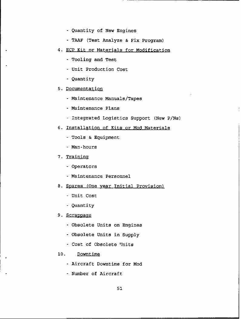
- Quantity of New Engines
- TAAF (Test Analyze & Fix Program)
4. ECP Kit or Materials for Modification
- Tooling and Test
- Unit Production Cost
- Quantity
5. Documentation
- Maintenance Manuals/Tapes
- Maintenance Plans
- Integrated Logistics Support (New P/Ns)
6. Installation of Kits or Mod Materials
- Tools & Equipment
- Man-hours
7. Training
- Operators
- Maintenance Personnel
8. Spares (One year Initial Provision)
- Unit Cost
- Quantity
9. Scrappage
- Obsolete Units on Engines
- Obsolete Units in Supply
- Cost of Obsolete Units
10. Downtime
- Aircraft Downtime for Mod
- Number of Aircraft
51
11. Testing
- Spin Tests
- Engine Tests
D. DISCUSSION OF THE EXPECTED COST SECTIONS
The expected cost section shows the calculations of costs
incurred both before and after the fix. The calculations are
broken down for inspections, end-of-life replacements,
unscheduled replacements, aircraft/personnel loss, and fuel
consumption. The formulas for each section are as follows
[Ref. 19:pp. 48-56]
Total Inspection costs equals I(MC+EJ) where:
I = Inspection frequency
M = MMH per Inspections
C = Cost per MMH
E = Elapsed Maintenance Time (EMT)3 per Inspection
J = Cost per NMC Hour
Total Replacement costs equals R(AC+P+BJ) where:
R = End-of-Life Replacement frequency
A = MMH per Replacement
C = Cost per MMH
P = Cost of Replacement Materials/Parts
3EMT is equal to the total maintenance time required toreturn the aircraft to mission-capable status. EMT is usuallyequivalent to NMC.
52
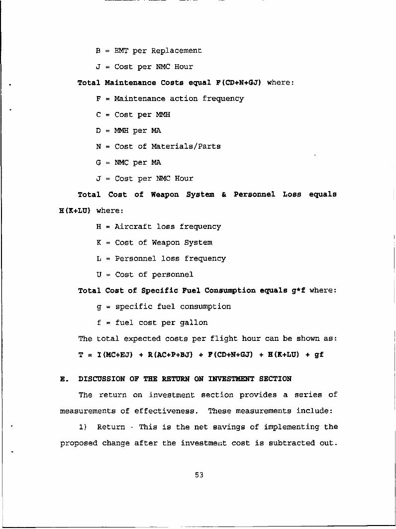
B = EMT per Replacement
J = Cost per NMC Hour
Total Maintenance Costs equal F(CD+N+GJ) where:
F = Maintenance action frequency
C = Cost per MMH
D = MMH per MA
N = Cost of Materials/Parts
G = NMC per MA
J = Cost per NMC Hour
Total Cost of Weapon System & Personnel Loss equals
H(K+LU) where:
H = Aircraft loss frequency
K = Cost of Weapon System
L = Personnel loss frequency
U = Cost of personnel
Total Cost of Specific Fuel Consumption equals g*f where:
g = specific fuel consumption
f = fuel cost per gallon
The total expected costs per flight hour can be shown as:
T = I(MC+EJ) + R(AC+P+BJ) + F(CD+N+GJ) + H(K+LU) + gf
E. DISCUSSION OF THE RETURN ON INVESTMENT SECTION
The return on investment section provides a series of
measurements of effectiveness. These measurements include:
1) Return - This is the net savings of implementing the
proposed change after the investmenit cost is subtracted out.
53
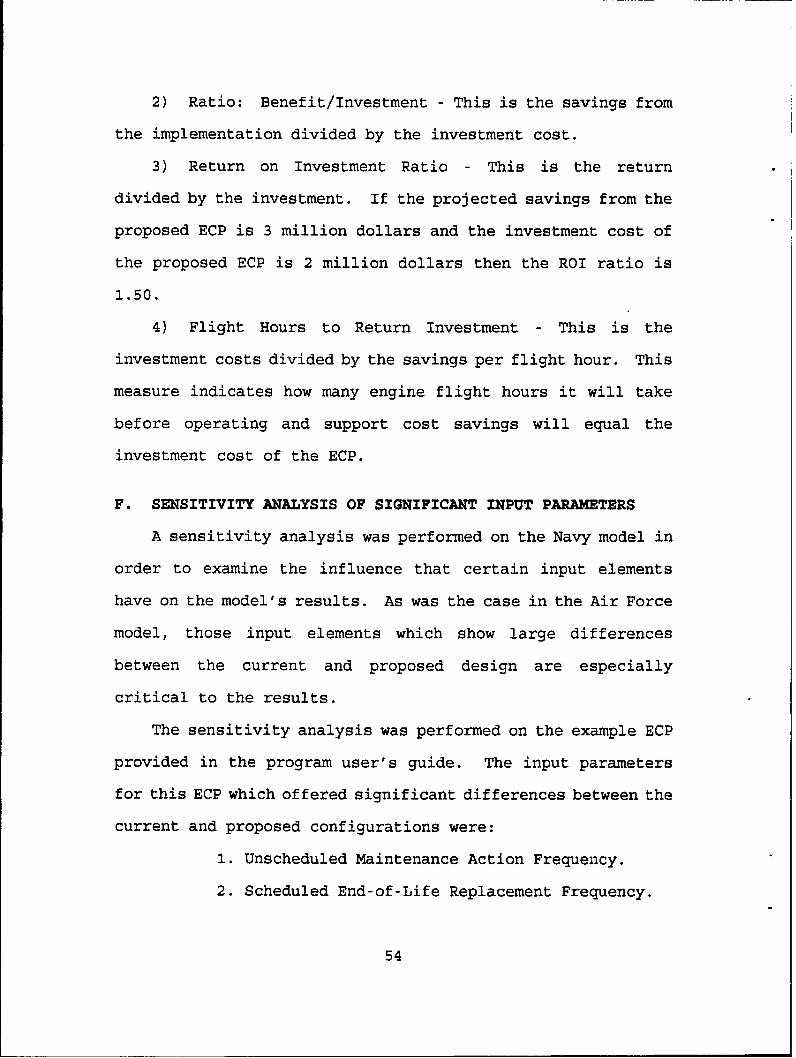
2) Ratio: Benefit/Investment - This is the savings from
the implementation divided by the investment cost.
3) Return on Investment Ratio - This is the return
divided by the investment. If the projected savings from the
proposed ECP is 3 million dollars and the investment cost of
the proposed ECP is 2 million dollars then the ROI ratio is
1.50.
4) Flight Hours to Return Investment - This is the
investment costs divided by the savings per flight hour. This
measure indicates how many engine flight hours it will take
before operating and support cost savings will equal the
investment cost of the ECP.
F. SENSITIVITY ANALYSIS OF SIGNIFICANT INPUT PARAMETERS
A sensitivity analysis was performed on the Navy model in
order to examine the influence that certain input elements
have on the model's results. As was the case in the Air Force
model, those input elements which show large differences
between the current and proposed design are especially
critical to the results.
The sensitivity analysis was performed on the example ECP
provided in the program user's guide. The input parameters
for this ECP which offered significant differences between the
current and proposed configurations were:
1. Unscheduled Maintenance Action Frequency.
2. Scheduled End-of-Life Replacement Frequency.
54

The sensitivity analysis attempted to determine the impact
which these parameters had on the model's results. The
selection of this ECP was purely for convenience.
As with the Air Force model, successive iterations of the
model were run while changing the proposed configuration's
input parameters in 10 percent increments toward the current
configuration's parameter values. The sensitivity analysis
varied the following prcposed input parameters: scheduled
end-of-life replacement frequency per EFH and unscheduled
maintenance action frequency rate.
Appendix B presents the original input parameters and the
results for each of the sensitivity analyses. Figure 3 on the
following page shows the results of the analysis. The results
showed that the input parameters had a significant effect on
the model's results. The author suggests a similar situation
to that of the Air Force model where there is a connection
between the component's reliability and the costs associated
with scheduled and unscheduled maintenance.
As with the Air Force model, the overall conclusion is
that the model's user must understand which particular input
parameters are driving the model's results and be sure to
concentrate on the accuracy of these input parameters.
55
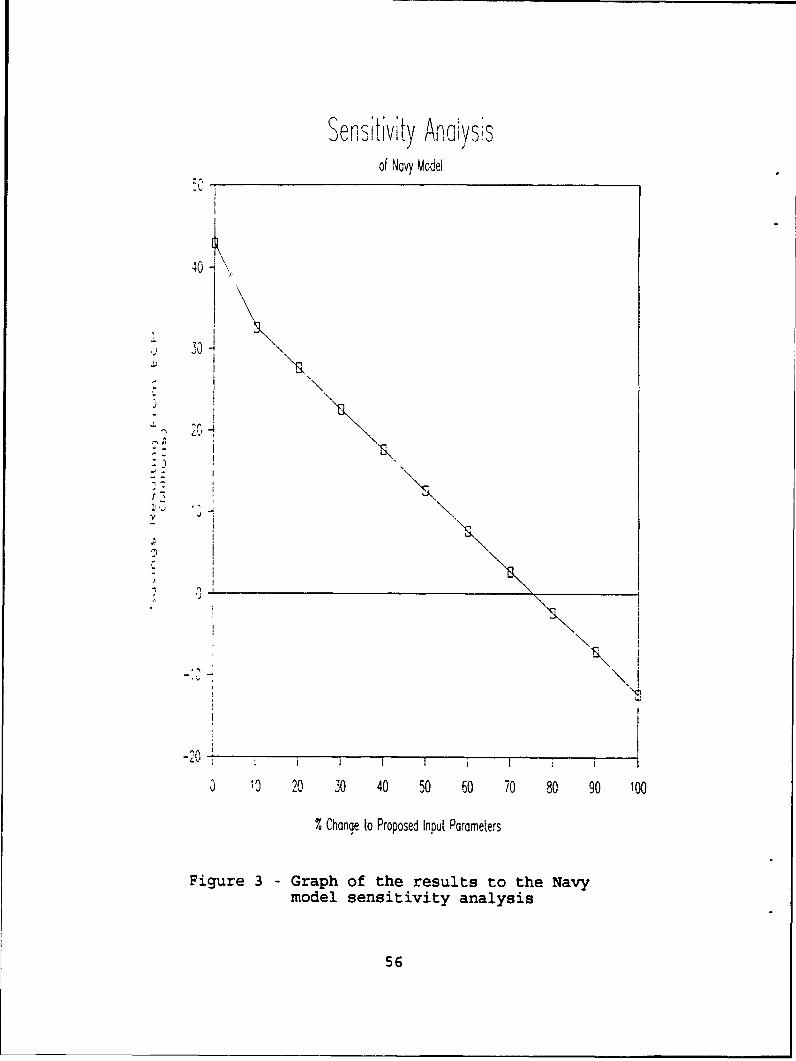
Se .sitiviiy Analysisof Novy Model
40 I,j 30 "U
- 7
- Is
-4
Y
I'll 20 310 40 50 60 70 80 90 100
%Change to Proposed Input Parameters
Figure 3 -Graph of the results to the Navymodel sensitivity analysis
56
G. DIFFERENCES BETWEEN THE AIR FORCE AND NAVY MODEL
Both models attempt to measure the change in LCC which
would result from implementing ECPs. The model developers
approached this task in similar fashion. Nevertheless, there
are significant differences between the models. The author
has identified four particular areas of difference which are:
Model Utilization - The Navy model is intended to examine
the entire CIP process and assist NAVAIR with the selection of
ECP development plans. This approach requires much more
forecasting to be done concerning the various costs.
The Air Force model is intended for use after the ECP has
been developed. The focus of this model is to assist in the
efficient allocation of ECP implementation funds. Since the
Air Force model is run at a later point than the Navy model,
the predicted costs estimates should be more fully developed.
Costs Concerns - Four costs which the Navy model examines
which are not part of the Air Force are: NMC costs; aircraft
loss costs; personnel loss costs; and scrappage costs. As
discussed earlier, the author feels that while NMC costs can
be significant, they are simply too difficult to measure. The
author is of the same opinion for aircraft and personnel loss
costs. The Navy needs to make much more progress in its
abilities to measure operating and support costs before it can
approach the tougher subjects of aircraft and personnel loss
costs.
The author strongly agrees with the inclusion of scrappage
57

costs in the Navy model. The scrappage costs fall under the
investment cost category and include the cost of obsolescence
of the replaced components on the aircraft engines and in the
supply system.
Costs which could be significant that show up in the Air
Force model are secondary damage costs. These costs covar
damages to other engine components caused by the failure of
the subject component. The relevance of this element
certainly depends on the specific component, but this input
parameter should be available for consideration in the models.
Input Parameter Format - The Air Force model goes into
much more detail concerning the operating and support costs.
The Air Force model devotes a great deal of effort in trying
to break costs down as far as possible. This is shown in
their effort to identify both the level of work required (0,
I or D) and the type of work required (inspection,
maintenance, repair/replace).
The Navy model is much simpler than the Air Force model in
this area. It breaks maintenance costs down into inspections
(which include all scheduled maintenance actions), and
unscheduled maintenance.
Measurements of Effectiveness - The Air Force model is
more concerned with the long-term return of the ECP
investment. All savings are calculated in terms of their net
present value. The savings are then added together and an
aggregate savings is shown in the results summary section.
58
The Navy model's presentation of the results does not
consider NPV and simply centers on the time it will take to
recoup the investment. Both models could be easily modified
to supply the same information.
59
VI. SUMMARY, CONCLUSIONS AND RECOMMENDATIONS
A. Summary
The question addressed in this thesis is whether it is
possible to accurately estimate the LCC savings for any
specific CIP efforts? A secondary concern has been the
comparison of the CIP cost-effectiveness models used by the
Air Force and Navy. In addition, are they good enough to
justify budget proposals to Congress?
To answer these questions the author first set out to
establish the framework of CIP. It became apparent that CIP
can achieve tremendous savings in aircraft engine operating
and support costs. However, it was also obvious that CIP
requires significant initial investments in order to design
and implement an engine component change.
In Chapter III, the author expounded on some basic
principles which should be considered when altering a system's
design in ciaer to improve LCC. The advantages and
limitations of modeling an LCC analysis were discussed as well
as some basic background terminology which is used in
describing these models.
Chapters IV and V specifically discussed the CIP cost-
effectiveness models used by the Air Force and Navy,
60
respectively. This included a discussion of the models' input
parameters and how they calculated their results.
A sensitivity analysis was performed on both models to
determine how responsive the models were to errors in the
proposed unscheduled and scheduled maintenance parameters.
Finally, the author made a direct comparison of the two
models. This comparison focused on: Model utilization; cost
concerns; input parameter format; and measurements of
effectiveness.
B. CONCLUSIONS
The benefits of CIP are without question. Unfortunately,
in order to rely on the models to justify CIP budget
proposals, we must be able to validate the results of the
models and prove with a significant level of certainty, their
accuracy. In the author's opinion, the lack of validation of
the Air Force and Navy models and their sensitivity to input
parameter errors prohibit them from being the primary basis
for CIP budgeting. This lack of validation is partly due to
the fact that the models have only recently been implemented
and partly due to the lack of resources available to perform
a validation of the models. Obviously, it would be extremely
risky to justify the Navy's CIP budget on the results of
models which have not been validated.
61
C. Recomendations
It is recommended that NAVAIR continue to use their
current ROI model to initially evaluate CIP proposals. In
addition, NAVAIR should consider developing a second ROI model
which does not include investment costs. This model would be
run after the development of the ECP but before its
implementation. This step would provide NAVAIR the
opportunity to update the LCC input data and determine if the
ECP implementation is still cost-effective. If the ECP does
not look to be cost-effective, it should be cancelled prior to
its implementation phase.
Both the Air Force and Navy models provide a framework
which can be used in developing a model which could be used
for budget justification. However, before this can occur the
services should closely examine their methods for determining
life-cycle costs and work closely in developing an accurate
means to measure and collect the relevant LCC data which would
be required for any model.
As just mentioned, there is the need to evaluate the
methods for determining life-cycle costs of aircraft engines.
One area which could be of significant interest would be the
validation of operating and support costs. These costs play
a significant role in both the Air Force and Navy models and
are, at the same time, the hardest factors to precisely
quantify.
62
APPENDIX A
AIR FORCE MODEL SENSITIVITY ANALYSIS
Appendix A shows the original and altered input parameters for
the ECP. The input parameters were altered in 10 percent
increments and are highlighted in the initial table for ease of
identification. The results summary section for each set of
variations is presented immediately following each iteration of the
input parameters.
63
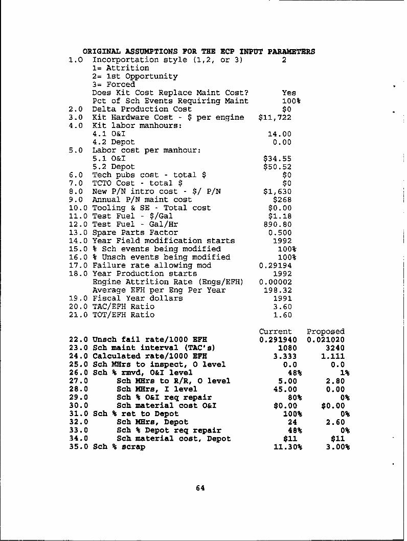
ORIGINAL ASSUMPTIONS FOR THE ECP INPUT PARAMETERS1.0 Incorportation style (1,2, or 3) 2
1= Attrition2= ist Opportunity3= ForcedDoes Kit Cost Replace Maint Cost? YesPct of Sch Events Requiring Maint 100%
2.0 Delta Production Cost $03.0 Kit Hardware Cost - $ per engine $11,7224.0 Kit labor manhours:
4.1 0&I 14.004.2 Depot 0.00
5.0 Labor cost per manhour:5.1 0&I $34.555.2 Depot $50.52
6.0 Tech pubs cost - total $ $07.0 TCTO Cost - total $ $08.0 New P/N intro cost - $/ P/N $1,6309.0 Annual P/N maint cost $26810.0 Tooling & SE - Total cost $0.0011.0 Test Fuel - $/Gal $1.1812.0 Test Fuel - Gal/Hr 890.8013.0 Spare Parts Factor 0.50014.0 Year Field modification starts 199215.0 % Sch events being modified 100%16.0 % Unsch events being modified 100%17.0 Failure rate allowing mod 0.2919418.0 Year Production starts 1992
Engine Attrition Rate (Engs/EFH) 0.00002Average EFH per Eng Per Year 198.32
19.0 Fiscal Year dollars 199120.0 TAC/EFH Ratio 3.6021.0 TOT/EFH Ratio 1.60
Current Proposed22.0 Unsch fail rate/1000 EFH 0.291940 0.02102023.0 Sch maint interval (TAC's) 1080 324024.0 Calculated rate/1000 EFH 3.333 1.11125.0 Sch MHrs to inspect, 0 level 0.0 0.026.0 Sch % rmvd, O&I level 48% 1%27.0 Sch MHrs to R/R, 0 level 5.00 2.8028.0 Sch MErs, I level 45.00 0.0029.0 Sch % 0&I req repair 80% 0%30.0 Sch material cost 0&I $0.00 $0.0031.0 Sch % ret to Depot 100% 0%32.0 Sch Mrs, Depot 24 2.6033.0 Sch % Depot req repair 48% 0%34.0 Sch material cost, Depot $11 $1135.0 Sch % scrap 11.30% 3.00%
64
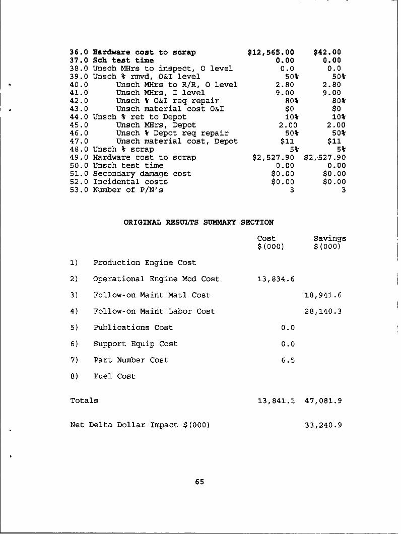
36.0 Hardware cost to scrap $12,565.00 $42.0037.0 Sch test time 0.00 0.0038.0 Unsch MHrs to inspect, 0 level 0.0 0.039.0 Unsch % rmvd, 0&I level 50% 50%40.0 Unsch MHrs to R/R, 0 level 2.80 2.8041.0 Unsch MHrs, I level 9.00 9.0042.0 Unsch % 0&I req repair 80% 80%43.0 Unsch material cost 0&I $0 $044.0 Unsch % ret to Depot 10% 10%45.0 Unsch MHrs, Depot 2.00 2.0046.0 Unsch % Depot req repair 50% 50%47.0 Unsch material cost, Depot $11 $1148.0 Unsch % scrap 5% 5%49.0 Hardware cost to scrap $2,527.90 $2,527.9050.0 Unsch test time 0.00 0.0051.0 Secondary damage cost $0.00 $0.0052.0 Incidental costs $0.00 $0.0053.0 Number of P/N's 3 3
ORIGINAL RESULTS SUMMARY SECTION
Cost Savings
$(000) $(000)
1) Production Engine Cost
2) Operational Engine Mod Cost 13,834.6
3) Follow-on Maint Matl Cost 18,941.6
4) Follow-on Maint Labor Cost 28,140.3
5) Publications Cost 0.0
6) Support Equip Cost 0.0
7) Part Number Cost 6.5
8) Fuel Cost
Totals 13,841.1 47,081.9
Net Delta Dollar Impact $(000) 33,240.9
65

ITERATION 1 PROPOSED UNSCHED AND SCHED MAINT PARAMETERSDECREASED 10%
Current Proposed22.0 Unsch fail rate/1000 EFH 0.291940 0.04811223.0 Sch maint interval (TAC's) 1080 302424.0 Calculated rate/1000 EFH 3.333 1.33326.0 Sch % rmvd, O&I level 48% 5.7%27.0 Sch MHrs to R/R, 0 level 5.00 3.0228.0 Sch MHrs, I level 45.00 4.5029.0 Sch % O&I req repair 80% 8%31.0 Sch % ret to Depot 100% 10%32.0 Sch MHrs, Depot 24 4.7433.0 Sch % Depot req repair 48% 4.8%35.0 Sch % scrap 11.30% 3.83%36.0 Hardware cost to scrap $12,565.00 $1294.30
RESULTS SUMMARY SECTION
Cost Savings
$(000) $(000)
1) Production Engine Cost
2) Operational Engine Mod Cost 13,834.6
3) Follow-on Maint Matl Cost 18,671.2
4) Follow-on Maint Labor Cost 27,919.0
5) Publications Cost 0.0
6) Support Equip Cost 0.0
7) Part Number Cost 6.5
8) Fuel Cost
Totals 13,841.1 46,590.2
Net Delta Dollar Impact $(000) 32,749.1
66
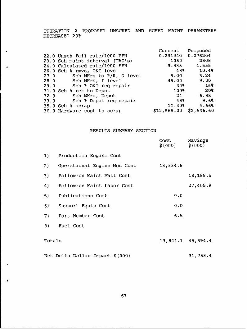
ITERATION 2 PROPOSED UNSCHED AND SCHED MAINT PARAMETERSDECREASED 20%
Current Proposed22.0 Unsch fail rate/1000 EFH 0.291940 0.07520423.0 Sch maint interval (TAC's) 1080 280824.0 Calculated rate/1000 EFH 3.333 1.55526.0 Sch W rmvd, O&I level 48% 10.4%27.0 Sch MHrs to R/R, 0 level 5.00 3.2428.0 Sch MHrs, I level 45.00 9.0029.0 Sch W O&I req repair 80% 16W31.0 Sch W ret to Depot 100% 20%32.0 Sch MHrs, Depot 24 6.8833.0 Sch % Depot req repair 48% 9.6%35.0 Sch % scrap 11.30% 4.66%36.0 Hardware cost to scrap $12,565.00 $2,546.60
RESULTS SUMMARY SECTIONCost Savings
$(000) $(000)
1) Production Engine Cost
2) Operational Engine Mod Cost 13,834.6
3) Follow-on Maint Matl Cost 18,188.5
4) Follow-on Maint Labor Cost 27,405.9
5) Publications Cost 0.0
6) Support Equip Cost 0.0
7) Part Number Cost 6.5
8) Fuel Cost
Totals 13,841.1 45,594.4
Net Delta Dollar Impact $(000) 31,753.4
67

ITERATION 3 PROPOSED UNSCHED AND SCHED MAINT PARAMETERSDECREASED 30%
Current Proposed22.0 Unsch fail rate/1000 EFH 0.291940 0.10229623.0 Sch maint interval (TAC's) 1080 259224.0 Calculated rate/1000 EFH 3.333 1.77826.0 Sch % rmvd, O&I level 48% 15.1%27.0 Sch MHrs to R/R, 0 level 5.00 3.4828.0 Sch MHrs, I level 45.00 13.5029.0 Sch W O&I req repair 80% 24%31.0 Sch % ret to Depot 100% 30%32.0 Sch MHrs, Depot 24 9.0233.0 Sch % Depot req repair 48% 14.4%35.0 Sch % scrap 11.30% 5.49%36.0 Hardware cost to scrap $12,565.00 $3,798.90
RESULTS SUMMARY SECTIONCost Savings
$(000) $(000)
1) Production Engine Cost
2) Operational Engine Mod Cost 13,834.6
3) Follow-on Maint Matl Cost 17,438.7
4) Follow-on Maint Labor Cost 26,503.2
5) Publications Cost 0.0
6) Support Equip Cost 0.0
7) Part Number Cost 6.5
8) Fuel Cost
Totals 13,841.1 43,941.9
Net Delta Dollar Impact $(000) 30,100.9
68
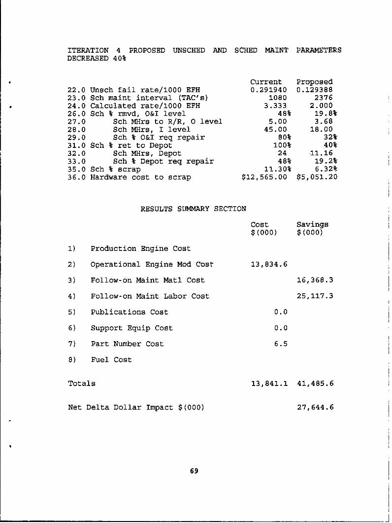
ITERATION 4 PROPOSED UNSCHED AND SCHED MAINT PARAMETERSDECREASED 40%
Current Proposed22.0 Unsch fail rate/1000 EFH 0.291940 0.12938823.0 Sch maint interval (TAC's) 1080 237624.0 Calculated rate/1000 EFH 3.333 2.00026.0 Sch % rmvd, O&I level 48% 19.8%27.0 Sch MHrs to R/R, 0 level 5.00 3.6828.0 Sch MHrs, I level 45.00 18.0029.0 Sch % 0&I req repair 80% 32%31.0 Sch % ret to Depot 100% 40%32.0 Sch MHrs, Depot 24 11.1633.0 Sch % Depot req repair 48% 19.2%35.0 Sch % scrap 11.30% 6.32%36.0 Hardware cost to scrap $12,565.00 $5,051.20
RESULTS SUMMARY SECTION
Cost Savings
$(000) $(000)
1) Production Engine Cost
2) Operational Engine Mod Cost 13,834.6
3) Follow-on Maint Matl Cost 16,368.3
4) Follow-on Maint Labor Cost 25,117.3
5) Publications Cost 0.0
6) Support Equip Cost 0.0
7) Part Number Cost 6.5
8) Fuel Cost
Totals 13,841.1 41,485.6
Net Delta Dollar Impact $(000) 27,644.6
69

ITERATION 5 PROPOSED UNSCHED AND SCHED MAINT PARAMETERSDECREASED 50%
Current Proposed22.0 Unsch fail rate/1000 EFH 0.291940 0.15648023.0 Sch maint interval (TAC's) 1080 216024.0 Calculated rate/1000 EFH 3.333 2.22226.0 Sch t rmvd, O&I level 48% 24.5%27.0 Sch MHrs to R/R, 0 level 5.00 3.9028.0 Sch MHrs, I level 45.00 22.5029.0 Sch W O&I req repair 80% 40%31.0 Sch W ret to Depot 100! 50%32.0 Sch MHrs, Depot 24 13.3033.0 Sch k Depot req repair 48% 24%35.0 Sch % scrap 11.30% 7.15%36.0 Hardware cost to scrap $12,565.00 $6,303.50
RESULTS SUMMARY SECTION
Cost Savings
$(000) $(000)
1) Production Engine Cost
2) Operational Engine Mod Cost 13,834.6
3) Follow-on Maint Matl Cost 14,922.7
4) Follow-on Maint Labor Cost 23,149.3
5) Publications Cost 0.0
6) Support Equip Cost 0.0
7) Part Number Cost 6.5
8) Fuel Cost
Totals 13,841.1 38,072.0
Net Delta Dollar Impact $(000) 24,231.0
70
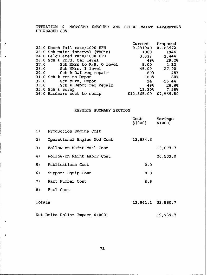
ITERATION 6 PROPOSED UNSCHED AND SCHED MAINT PARAMETERSDECREASED 60%
Current Proposed22.0 Unsch fail rate/1000 EFH 0.291940 0.18357223.0 Sch maint interval (TAC's) 1080 194424.0 Calculated rate/1000 EFH 3.333 2.44426.0 Sch % rmvd, O&I level 48% 29.2%27.0 Sch MHrs to R/R, 0 level 5.00 4.1228.0 Sch MHrs, I level 45.00 27.0029.0 Sch % O&I req repair 80% 48%31.0 Sch W ret to Depot 100% 60%32.0 Sch MHrs, Depot 24 15.4433.0 Sch t Depot req repair 48% 28.8%35.0 Sch k scrap 11.30% 7.98%36.0 Hardware cost to scrap $12,565.00 $7,555.80
RESULTS SUMMARY SECTION
Cost Savings
$(000) $(000)
1) Production Engine Cost
2) Operational Engine Mod Cost 13,834.6
3) Follow-on Maint Matl Cost 13,077.7
4) Follow-on Maint Labor Cost 20,503.0
5) Publications Cost 0.0
6) Support Equip Cost 0.0
7) Part Number Cost 6.5
8) Fuel Cost
Totals 13,841.1 33,580.7
Net Delta Dollar Impact $(000) 19,739.7
71
ITERATION 7 PROPOSED UNSCHED AND SCHED MAINT PARAMETERSDECREASED 70%
Current Proposed22.0 Unsch fail rate/1000 EFH 0.291940 0.21066423.0 Sch maint interval (TAC's) 1080 172824.0 Calculated rate/1000 EPH 3.333 2.66626.0 Sch % rmvd, O&I level 48% 33.9%27.0 Sch MHrs to R/R, 0 level 5.00 4.3428.0 Sch MHrs, I level 45.00 31.5029.0 Sch % O&I req repair 80% 56%31.0 Sch % ret to Depot 100% 70%32.0 Sch MHrs, Depot 24 .17.5833.0 Sch % Depot req repair 48% 33.6%35.0 Sch % scrap 11.30% 8.81%36.0 Hardware cost to scrap $12,565.00 $8,808.10
RESULTS SUMMARY SECTION
Cost Savings$(000) $(000)
1) Production Engine Cost
2) Operational Engine Mod Cost 13,834.6
3) Follow-on Maint Matl Cost 10,726.6
4) Follow-on Maint Labor Cost 17,081.6
5) Publications Cost 0.0
6) Support Equip Cost 0.0
7) Part Number Cost 6.5
8) Fuel Cost
Totals 13,841.1 27,808.2
Net Delta Dollar Impact $(000) 13,967.2
72
ITERATION 8 PROPOSED UNSCHED AND SCHED MAINT PARAMETERSDECREASED 80%
Current Proposed22.0 Unsch fail rate/1000 EFH 0.291940 0.23775623.0 Sch maint interval (TAC's) 1080 151224.0 Calculated rate/1000 EFH 3.333 2.88926.0 Sch % rmvd, O&I level 48% 38.6%27.0 Sch MHrs to R/R, 0 level 5.00 4.5628.0 Sch MHrs, I level 45.00 36.0029.0 Sch % O&I req repair 80% 64%31.0 Sch % ret to Depot 100% 80%32.0 Sch MHrs, Depot 24 19.7233.0 Sch % Depot req repair 4S% 38.4%35.0 Sch % scrap 11.30% 9.64%36.0 Hardware cost to scrap $12,565.00 $10,060.40
RESULTS SUMMARY SECTIONCost Savings
$(000) $(000)
1) Production Engine Cost
2) Operational Engine Mod Cost 13,834.6
3) Follow-on Maint Matl Cost 7,880.0
4) Follow-on Maint Labor Cost 12,783.7
5) Publications Cost 0.0
6) Support Equip Cost 0.0
7) Part Number Cost 6.5
8) Fuel Cost
Totals 13,841.1 20,663.7
Net Delta Dollar Impact $(000) 6,822.6
73
ITERATION 9 PROPOSED UNSCHED AND SCHED MAINT PARAMETERSDECREASED 90%
Current Proposed22.0 Unsch fail rate/1000 EFH 0.291940 0.26484823.0 Sch maint interval (TAC's) 1080 129624.0 Calculated rate/1000 EFH 3.333 3.11126.0 Sch t rmvd, O&I level 48% 43.3%27.0 Sch MHrs to R/R, 0 level 5.00 4.7828.0 Sch MHrs, I level 45.00 40.5029.0 Sch t O&I req repair 80% 72%31.0 Sch % ret to Depot 100% 90%32.0 Sch MHrs, Depot 24 21.8633.0 Sch t Depot req repair 48% 43.2%35.0 Sch W scrap 11.30% 10.47%36.0 Hardware cost to scrap $12,565.00 $11,312.70
RESULTS SUMMARY SECTION
Cost Savings
$(000) $(000)
1) Production Engine Cost
2) Operational Engine Mod Cost 13,834.6
3) Follow-on Maint Matl Cost 4,353.1
4) Follow-on Maint Labor Cost 7,521.3
5) Publications Cost 0.0
6) Support Equip Cost 0.0
7) Part Number Cost 6.5
8) Fuel Cost
Totals 13,841.1 11,874.4
Net Delta Dollar Impact $(000) 1,966.7
(Tuis impact results in a net cost of $1,966,700)
74
ITERATION 10 PROPOSED UNSCHED AND SCHED MAINT PARAMETERSDECREASED 100%
Current Proposed22.0 Unsch fail rate/1000 EFH 0.291940 0.29194023.0 Sch maint interval (TAC's) 1080 108024.0 Calculated rate/1000 EFH 3.333 3.33326.0 Sch % rmvd, O&I level 48% 48%27.0 Sch MHrs to R/R, 0 level 5.00 5.0028.0 Sch MHrs, I level 45.00 45.0029.0 Sch % O&I req repair 80% 80%31.0 Sch % ret to Depot 100% 100%32.0 Sch MHrs, Depot 24 2433.0 Sch % Depot req repair 48% 48%35.0 Sch % scrap 11.30% 11.30%36.0 Hardware cost to scrap $12,565.00 $12,565.00
RESULTS SUMMARY SECTIONCost Savings
$(000) $(000)
1) Production Engine Cost
2) Operational Engine Mod Cost 13,834.6
3) Follow-on Maint Matl Cost 99.9
4) Follow-on Maint Labor Cos'_ 1,013.4
5) Publications Cost 0.0
6) Support Equip Cost 0.0
7) Part Number Cost 6.5
8) Fuel Cost
Totals 13,841.1 1,113.4
Net Delta Dollar Impact $(000) 12,727.7
(This impact results in a net cost of $12,727,700)
75
APPENDIX B
NAVY ROI MODEL SENSITIVITY ANALYSIS
Appendix B shows the original and altered input parameters for
the ECP. The input parameters were altered in 10 percent
increments and are highlighted in the initial table for ease of
identification. The return-on-investment section for each set of
variations is presented immediately following each iteration of the
input parameters.
76
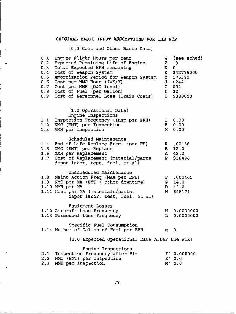
ORIGINAL BASIC INPUT ASSUMPTIONS FOR THE ECP
[0.0 Cost and Other Basic Data]
0.1 Engine Flight Hours per Year W (see sched)0.2 Expected Remaining Life of Engine Z 130.3 Total Expected EFH remaining X 00.4 Cost of Weapon System K $427750000.5 Amortization Period for Weapon System Y 1753200.6 Cost per NMC Hour (J=K/Y) J $2440.7 Cost per MMH (O&I level) C $310.8 Cost of Fuel (per Gallon) f $00.9 Cost of Personnel Loss (Train Costs) U $330000
[1.0 Operational Data]Engine Inspections
1.1 Inspection Frequency (Insp per EFH) I 0.001.2 NMC (EMT) per Inspection E 0.001.3 MMH per Inspection M 0.00
Scheduled Maintenance1.4 End-of-Life Replace Freq. (per FH) R .001361.5 NMC (EMT) per Replace B 12.01.6 MMH per Replacement A 42.01.7 Cost of Replacement (material/parts P $36496
depot labor, test, fuel, et al)
Unscheduled Maintenance1.8 Maint Action Freq (MAs per EFH) F .0004651.9 NMC per MA (EMT + cther downtime) G 14.01.10 MMH per MA D 42.01.11 Cost per MA (materials/parts, N $48171
depot labor, test, fuel, et al)
Equipment Losses1.12 Aircraft Loss Frequency H 0.00000001.13 Personnel Loss Frequency L 0.0000000
Specific Fuel Consumption
1.14 Number of Gallon of Fuel per EFH g 0
[2.0 Expected Operational Data After the Fix]
Engine Inspections2.1 Inspectin Frequency after Fix I' 0.0000002.2 NMC (ELM-T) per Inspection E' 0.02.3 MMH per Inspectio; M' 0.0
77
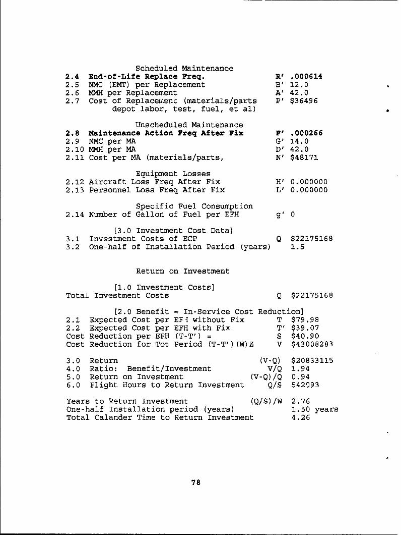
Scheduled Maintenance2.4 End-of-Life Replace Freq. R' .0006142.5 NMC (EMT) per Replacement B' 12.02.6 MMH per Replacement A' 42.02.7 Cost of Replacemenc (materials/parts P' $36496
depot labor, test, fuel, et al)
Unscheduled Maintenance2.8 Maintenance Action Freq After Fix F' .0002662.9 NMC per MA G' 14.02.10 MMH per MA D' 42.02.11 Cost per MA (materials/parts, N' $48171
Equipment Losses2.12 Aircraft Loss Freq After Fix H' 0.0000002.13 Personnel Loss Freq After Fix L' 0.000000
Specific Fuel Consumption2.14 Number of Gallon of Fuel per EFH g' 0
[3.0 Investment Cost Data]3.1 Investment Costs of ECP Q $221751683.2 One-half of Installation Period (years) 1.5
Return on Investment
[1.0 Investment Costs]Total Investment Costs Q $22175168
[2.0 Benefit = In-Service Cost Reduction]2.1 Expected Cost per EF{ without Fix T $79.982.2 Expected Cost per EFH with Fix T' $39.07Cost Reduction per EFH (T-T') = S $40.90Cost Reduction for Tot Period (T-T') (W)Z V $43008283
3.0 Return (V-Q) $208331154.0 Ratio: Benefit/Investment V/Q 1.945.0 Return on Investment (V-Q)/Q 0.946.0 Flight Hours to Return Investment Q/S 542093
Years to Return Investment (Q/S)/W 2.76One-half Installation period (years) 1.50 yearsTotal Calander Time to Return Investment 4.26
78

FLIGHT HOUR SCHEDULE
Number of Years in Schedule: 13First Year: 1988
* Year FLT. HRS. CUM. HRS.
1988 207,000 207,0001989 194,400 401,4001990 185,400 586,8001)91 174,060 760,8601992 157,320 918,1801993 133,740 1,051,9201994 105,660 1,157,5801995 75,060 1,232,6401996 48,240 1,280,8801997 33,660 1,314,5401998 23,760 1,338,3001999 12,960 1,351,2602000 4,320 1,355,580
79
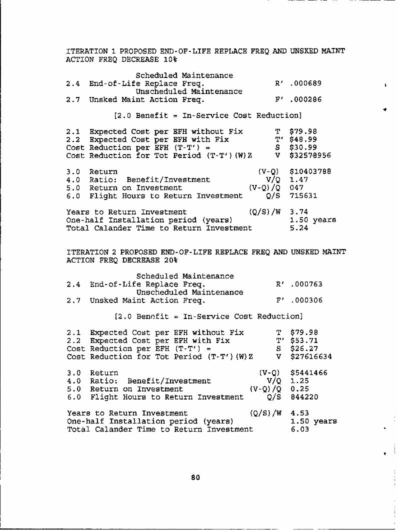
ITERATION 1 PROPOSED END-OF-LIFE REPLACE FREQ AND UNSKED MAINTACTION FREQ DECREASE 10%
Scheduled Maintenance2.4 End-of-Life Replace Freq. R' .000689
Unscheduled Maintenance2.7 Unsked Maint Action Freq. F' .000286
(2.0 Benefit = In-Service Cost Reduction]
2.1 Expected Cost per EFH without Fix T $79.982.2 Expected Cost per EFH with Fix T' $48.99Cost Reduction per EFH (T-T') = S $30.99Cost Reduction for Tot Period (T-T') (W)Z V $3257-8956
3.0 Return (V-Q) $104037884.0 Ratio: Benefit/Investment V/Q 1.475.0 Return on Investment (V-Q)/Q 0476.0 Flight Hours to Return Investment Q/S 715631
Years to Return Investment (Q/S)/W 3.74One-half Installation period (years) 1.50 yearsTotal Calander Time to Return Investment 5.24
ITERATION 2 PROPOSED END-OF-LIFE REPLACE FREQ AND UNSKED MAINTACTION FREQ DECREASE 20%
Scheduled Maintenance2.4 End-of-Life Replace Freq. R' .000763
Unscheduled Maintenance2.7 Unsked Maint Action Freq. F' .000306
[2.0 Benefit = In-Service Cost Reduction]
2.1 Expected Cost per EFH without Fix T $79.982.2 Expected Cost per EFH with Fix T' $53.71Cost Reduction per EFH (T-T') = S $26.27Cost Reduction for Tot Period (T-T') (W)Z V $27616634
3.0 Return (V-Q) $54414664.0 Ratio: Benefit/Investment V/Q 1.255.0 Return on Investment (V-Q)/Q 0.256.0 Flight Hours to Return Investment Q/S 844220
Years to Return Investment (Q/S)/W 4.53One-half Installation period (years) 1.50 yearsTotal Calander Time to Return Investment 6.03
80

ITERATION 3 PROPOSED END-OF-LIFE REPLACE FREQ AND UNSKED MAINTACTION FREQ DECREASE 30%
Scheduled Maintenance2.4 End-of-Life Replace Freq. R' .000838
Unscheduled Maintenance2.7 Unsked Maint Action Freq. F' .000326
[2.0 Benefit = In-Service Cost Reduction]
2.1 Expected Cost per EFH without Fix T $79.982.2 Expected Cost per EFH with Fix T' $58.48Cost Reduction per EFH (T-T') = S $21.50Cost Reduction for Tot Period (T-T')(W)Z V $22601630
3.0 Return (V-Q) $4264624.0 Ratio: Benefit/Investment V/Q 1.025.0 Return on Investment (V-Q)/Q 0.026.0 Flight Hours to Return Investment Q/S 1031541
Years to Return Investment (Q/S)/W 5.85One-half Installation period (years) 1.50 yearsTotal Calander Time to Return Investment 7.35
ITERATION 4 PROPOSED END-OF-LIFE REPLACE FREQ AND UNSKED MAINTACTION FREQ DECREASE 40%
Scheduled Maintenance2.4 End-of-Life Replace Freq. R' .000912
Unscheduled Maintenance2.7 Unsked Maint Action Freq. F' .000346
[2.0 Benefit = In-Service Cost Reducticn]
2.1 Expected Cost per EFH without Fix T $79.982.2 Expected Cost per EFH with Fix T' $63.20Cost Reduction per EFH (T-T') = S $16.77Cost Reduction for Tot Period (T T) (W)Z V $17639308
3.0 Return (V-Q) $(4535859)4.0 Ratio: Benefit/Investment V/Q 0.805.0 Return on Investment (V-Q)/Q (.20)6.0 Flight Hours to Return Investment Q/S 1321737
Years to Return Investment (Q/S)/W 10.30One-half Installation period (years) 1.50 yearsTotal Calander Time to Return Investment 11.80
81
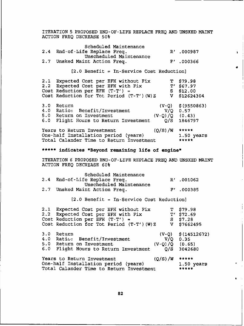
ITERATION 5 PROPOSED END-OF-LIFE REPLACE FREQ AND UNSKED MAINTACTION FREQ DECREASE 50%
Scheduled Maintenance2.4 End-of-Life Replace Freq. R' .000987
Unscheduled Maintenance2.7 Unsked Maint Action Freq. F' .000366
[2.0 Benefit = In-Service Cost Reduction]
2.1 Expected Cost per EFH without Fix T $79.982.2 Expected Cost per EFH with Fix T' $67.97Cost Reduction per EFH (T-T') = S $12.00Cost Reduction for Tot Period (T-T') (W)Z V $12624304
3.0 Return (V-Q) $(9550863)4.0 Ratio: Benefit/Investment V/Q 0.575.0 Return on Investment (V-Q)/Q (0.43)6.0 Flight Hours to Return Investment Q/S 1846797
Years to Return Investment (Q/S)/W ****
One-half Installation period (years) 1.50 yearsTotal Calander Time to Return Investment
***** indicates "Beyond remaining life of engine"
ITERATION 6 PROPOSED END-OF-LIFE REPLACE FREQ AND UNSKED MAINTACTION FREQ DECREASE 60%
Scheduled Maintenance2.4 End-of-Life Replace Freq. R' .001062
Unscheduled Maintenance2.7 Unsked Maint Action Freq. F' .000385
[2.0 Benefit = In-Service Cost Reduction]
2.1 Expected Cost per EFH withoat Fix T $79.982.2 Expected Cost per EFH with Fix T' $72.69Cost Reduction per EFH (T-T') = S $7.28Cost Reduction for Tot Period (T-T') (W)Z V $7662495
3.0 Return (V-Q) $(14512672)4.0 Ratio: Benefit/Investment V/Q 0.355.0 Return on Investment (V-Q)/Q (0.65)6.0 Flight Hours to Return Investment Q/S 3042680
Years to Return Investment (Q/S)/W *****One-half Installation period (years) 1.50 yearsTotal Calander Time to Return Investment
82
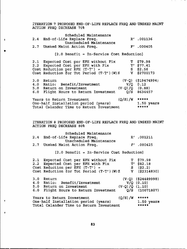
ITERATION 7 PROPOSED END-OF-LIFE REPLACE FREQ AND UNSKED MAINTACTION FREQ DECREASE 70%
Scheduled Maintenance2.4 End-of-Life Replace Freq. R' .001136
Unscheduled Maintenance2.7 Unsked Maint Action Freq. F' .000405
9
[2.0 Benefit = In-Service Cost Reduction]
2.1 Expected Cost per EFH without Fix T $79.982.2 Expected Cost per EFH with Fix T' $77.41Cost Reduction per EFH (T-T') = S $2.56Cost Reduction for Tot Period (T-T')(W)Z V $2700173
3.0 Return (V-Q) ($19474994)4.0 Ratio: Benefit/Investment V/Q 0.125.0 Return on Investment (V-Q)/Q (0.88)6.0 Flight Hours to Return Investment Q/S 8634457
Years to Return Investment (Q/S)/W *****One-half Installation period (years) 1.50 yearsTotal Calander Time to Return Investment
ITERATION 8 PROPOSED END-OF-LIFE REPLACE FREQ AND UNSKED MAINTACTION FREQ DECREASE 80%
Scheduled Maintenance2.4 End-of-Life Replace Freq. R' .001211
Unscheduled Maintenance2.7 Unsked Maint Action Freq. F' .000425
[2.0 Benefit = In-Service Cost Reduction]
2.1 Expected Cost per EFH without Fix T $79.982.2 Expected Cost per EFH with Fix T' $82.18Cost Reduction per EFH (T-T') = S ($2.2)Cost Reduction for Tot Period (T-T') (W)Z V ($2314830)
3.0 Return (V-Q) ($24489998)4.0 Ratio: Benefit/Investment V/Q (0.10)5.0 Return on Investment (V-Q)/Q (1.10)6.0 Flight Hours to Return Investment Q/S (10071807)
Years to Return Investment (Q/S)/W *****One-half Installation period (years) 1.50 yearsTotal Calander Time to Return Investment
83
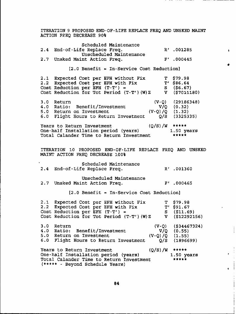
ITERATION 9 PROPOSED END-OF-LIFE REPLACE FREQ AND UNSKED MAINTACTION FREQ DECREASE 90%
Scheduled Maintenance2.4 End-of-Life Replace Freq. R' .001285
Unscheduled Maintenance2.7 Unsked Maint Action Freq. F' .000445
[2.0 Benefit = In-Service Cost Reduction]
2.1 Expected Cost per EFH without Fix T $79.982.2 Expected Cost per EFH with Fix T' $86.64Cost Reduction per EFH (T-T') = S ($6.67)Cost Reduction for Tot Period (T-T') (W)Z V ($7011180)
3.0 Return (V-Q) (29186348)4.0 Ratio: Benefit/Investment V/Q (0.32)5.0 Return on Investment (V-Q)/Q (1.32)6.0 Flight Hours to Return Investment Q/S (3325335)
Years to Return Investment (Q/S)/W *****One-half Installation period (years) 1.50 yearsTotal Calander Time to Return Investment
ITERATION 10 PROPOSED END-OF-LIFE REPLACE FREQ AND UNSKEDMAINT ACTION FREQ DECREASE 100%
Scheduled Maintenance2.4 End-of-Life Replace Freq. R' .001360
Unscheduled Maintenance
2.7 Unsked Maint Action Freq. F' .000465
[2.0 Benefit = In-Service Cost Reduction]
2.1 Expected Cost per EFH without Fix T $79.982.2 Expected Cost per EFH with Fix T' $91.67Cost Reduction per EFH (T-T') = S ($11.69)Cost Reduction for Tot Period (T-T') (W)Z V ($12292156)
3.0 Return (V-Q) ($34467324)4.0 Ratio: Benefit/Investment V/Q (0.55)5.0 Return on Investment (V-Q)/Q (1.55)6.0 Flight Hours to Return Investment Q/S (1896699)
Years to Return Investment (Q/S)/W *****One-half Installation period (years) 1.50 yearsTotal Calander Time to Return Investment
* Beyond Schedule Years)
84
LIST OF REFERENCES
I. Nelson, J. R., Harmon, B. R., and Tyson, K. W., "PolicyOptions for the Aircraft Turbine Engine Component ImprovementProgram", Institute for Defense Analyses, Alexandria, VA, May1987.
2. "Acquisition Plan AP No. A42-48-0-50 Rev B for AircraftEngine Component Improvement Program", Naval Air SystemsCommand, Washington, D.C., August 1987.
3. "Policy Guidelines and Responsibilities for theAdministration of the Aircraft Engine Component ImprovementProgram", NAVAIR Instruction 5200.35, Naval Air SystemsCommand, Washington, D.C., 25 January 1982.
4. "Military Standard 2173(AS) Reliability-CenteredMaintenance Requirements for Naval Aircraft, Weapon Systemsand Support Equipment", Department of Defense, Washington,D.C., August 1981.
5. "Program Management Plan for the Engine ComponentImprovement Program", Air Force Systems Command, United StatesAir Force, Acquisition Support Division, Wright Patters;on AirForce Base, OH, 10 March 1989.
6. "Component Improvement Program Technical Evaluation Plan",Naval Air Systems Command, Washington, D.C., 21 June 1988.
7. "Engine Component Improvement Feedback Report (ECIFR)";Naval Air Systems Command, Washington, D.C., March 1989.
8. Blanchard, Benj.min S., Logistics Engineering andManangement. 3rd edition, Prentice-Hall, Englewood Cliffs, NewJersey, 1986.
9. Davidson, Sidney, Stickney, Clyde P., and Weil, Roman L.,Financial Accounting: An Introduction to Concepts. Methods.and Uses, 5th edition, Dryden Press, Chicago, 1988.
10. Office of Management and Budget, Circular No. A-94,Washington, D.C., 1972.
11. Turban, Efraim, Decision Support and Expert Systems:Management Support Systems, 2nd edition, Macmillian PublishingCompany, New York, 1990.
85
12. Department of Defense; DOD Instruction 5000.2, "DefenseAcquisition Management Policies and Procedures", 1 January1991.
13. Isaacson, Donald, "Life Cycle Cost Analysis, in theReliability, Maintainability, and Supportability Guidebook",Society of Automotive Engineers, Inc., Warrendale, PA, 1990.
14. Davidson, George H., Capt, USAF and Griffiths, Raymond E.,Capt, USAF, "An Identification and Characterization of CostModels/Techniques Used by Air Force Logistics Command toEstimate Jet Engine Operation and Support Costs"; Air ForceInstitute of Technology, Wright Patterson Air Force Base, OH;June 1977.
15. Nelson, J.R., "An Approach To The Life-Cycle Analysis OfAircraft Turbine Engines, in the Application of Design to Costand Life Cycle Cost to Aircraft Engines", AGARD Series No.107, May 1980.
16. Minnick, Arthur E., "Life Cycle Cost Management, in theReliability, Mairtainability, and Supportability Guidebook",Society of Autom.-:ive Engineers, Inc., Warrendale, PA, 1990.
17. Francke, K. P., "User's Manual, Cost EffectivenessAnalysis Model for Program Task Plan and Engineering ChangeProposals", United Technologies Corp, West Palm Beach, FL,March 1989.
18. Telephone Conversation between John Blakley, AircraftEngine Group, General Electric Company and the author onNovember 7, 1991.
19. "AIR-536 Return-on-Investment Analysis Program User'sGuide", Naval Air Systems Command, Washington, D.C., September1989.
86
INITIAL DISTRIBUTION LISTNo. Copies
1. Defense Technical Information Center 2e Cameron Station
Alexandria, Virginia 22304-6145
2. Library, Code 0142 2Naval Postgraduate SchoolMonterey, California 93943-6145
3. Defense Logistics Studies 1Information ExchangeU.S. Army Logistics Management CenterFort Lee, Virginia 23801-6043
4. Commander 5Naval Air Systems CommandCode 536BWashington, DC 20361-5360
5. Aeronautical Systems Division ICode: ASD/YZLRAttn: S. McDonaldWright Patterson Air Force Base, Ohio 45433
6. Professor Alan W. McMasters, Code AS/MG 2Department of Administrative SciencesNaval Postgraduate SchoolMonterey, California 93943-5000
7. Professor Kishore Sengupta, Code AS/SE 1Department of Administrative SciencesNaval Postgraduate SchoolMonterey, California 93943-5000
8. LT James D. Davis 1252 Seville BlvdSayville, NY 11782
87