Montgomery: Chapter 4 Lecture 6: Block Designsyuzhu/stat514s2006/Lecnot/blockdesigns2006... · Lecture 6: Block Designs Montgomery: Chapter 4 Spring, 2006 Page 1. Statistics 514:

Statistics 514: Block Designs

Lecture 6: Block Designs

Montgomery: Chapter 4

Spring, 2006Page 1


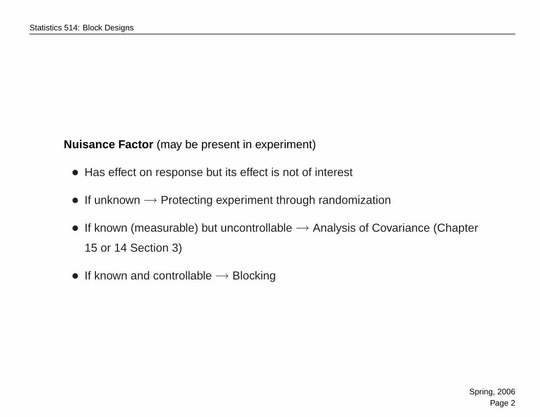
Nuisance Factor (may be present in experiment)

• Has effect on response but its effect is not of interest

• If unknown → Protecting experiment through randomization

• If known (measurable) but uncontrollable → Analysis of Covariance (Chapter

15 or 14 Section 3)

• If known and controllable → Blocking

Spring, 2006Page 2


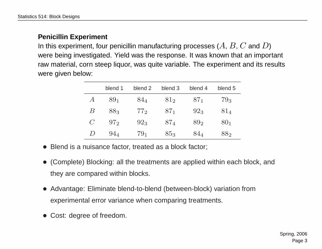
Penicillin ExperimentIn this experiment, four penicillin manufacturing processes (A, B, C and D)were being investigated. Yield was the response. It was known that an importantraw material, corn steep liquor, was quite variable. The experiment and its resultswere given below:

blend 1 blend 2 blend 3 blend 4 blend 5

A 891 844 812 871 793

B 883 772 871 923 814

C 972 923 874 892 801

D 944 791 853 844 882

• Blend is a nuisance factor, treated as a block factor;

• (Complete) Blocking: all the treatments are applied within each block, and

they are compared within blocks.

• Advantage: Eliminate blend-to-blend (between-block) variation from

experimental error variance when comparing treatments.

• Cost: degree of freedom.

Spring, 2006Page 3


Randomized Complete Block Design

• b blocks each consisting of (partitioned into) a experimental units

• a treatments are randomly assigned to the experimental units within each

block

• Typically after the runs in one block have been conducted, then move to

another block.

• Typical blocking factors: day, batch of raw material etc.

• Results in restriction on randomization because randomization is only within

blocks.

• Data within a block are dependent on each other. When a = 2, randomized

complete block design becomes paired two sample case.

Spring, 2006Page 4


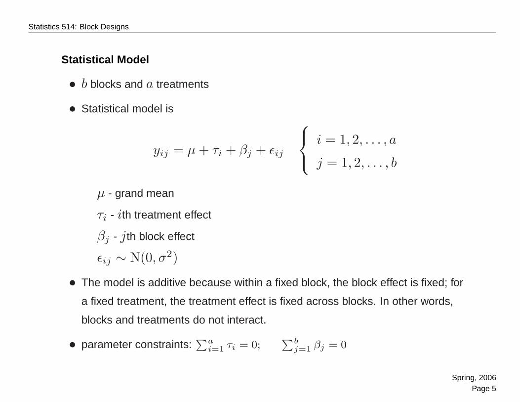
Statistical Model

• b blocks and a treatments

• Statistical model is

yij = µ + τi + βj + εij

i = 1, 2, . . . , a

j = 1, 2, . . . , b

µ - grand mean

τi - ith treatment effect

βj - jth block effect

εij ∼ N(0, σ2)

• The model is additive because within a fixed block, the block effect is fixed; for

a fixed treatment, the treatment effect is fixed across blocks. In other words,

blocks and treatments do not interact.

• parameter constraints:∑a

i=1 τi = 0;∑b

j=1 βj = 0

Spring, 2006Page 5


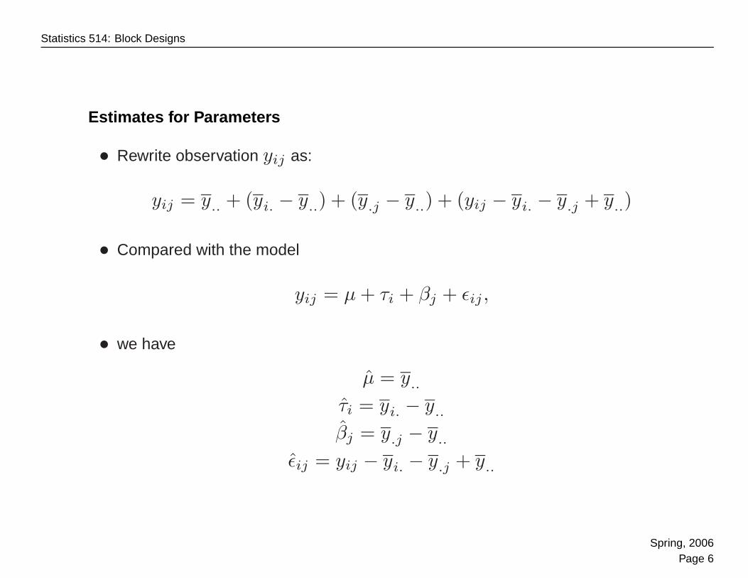
Estimates for Parameters

• Rewrite observation yij as:

yij = y.. + (yi. − y..) + (y.j − y..) + (yij − yi. − y.j + y..)

• Compared with the model

yij = µ + τi + βj + εij ,

• we have

µ = y..

τi = yi. − y..

βj = y.j − y..

εij = yij − yi. − y.j + y..

Spring, 2006Page 6


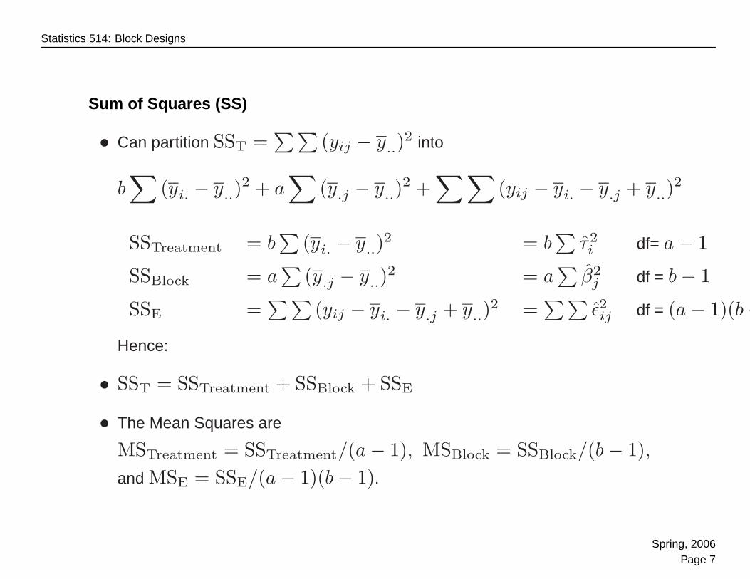
Sum of Squares (SS)

• Can partition SST =∑ ∑

(yij − y..)2 into

b∑

(yi. − y..)2 + a

∑(y.j − y..)

2 +∑ ∑

(yij − yi. − y.j + y..)2

SSTreatment = b∑

(yi. − y..)2 = b∑

τ2i df= a − 1

SSBlock = a∑

(y.j − y..)2 = a∑

β2j df = b − 1

SSE =∑ ∑

(yij − yi. − y.j + y..)2 =∑ ∑

ε2ij df = (a − 1)(b −Hence:

• SST = SSTreatment + SSBlock + SSE

• The Mean Squares are

MSTreatment = SSTreatment/(a − 1), MSBlock = SSBlock/(b − 1),and MSE = SSE/(a − 1)(b − 1).

Spring, 2006Page 7


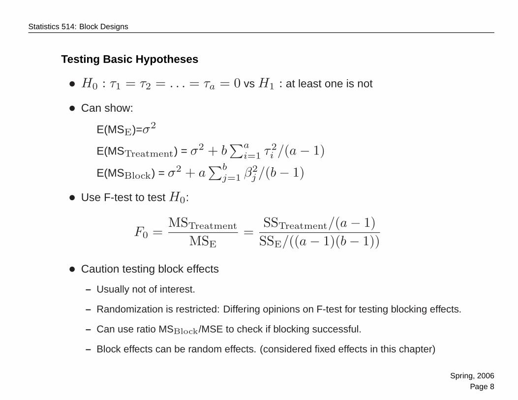
Testing Basic Hypotheses

• H0 : τ1 = τ2 = . . . = τa = 0 vs H1 : at least one is not

• Can show:

E(MSE)=σ2

E(MSTreatment) = σ2 + b∑a

i=1 τ2i /(a − 1)

E(MSBlock) = σ2 + a∑b

j=1 β2j /(b − 1)

• Use F-test to test H0:

F0 =MSTreatment

MSE=

SSTreatment/(a − 1)SSE/((a − 1)(b − 1))

• Caution testing block effects

– Usually not of interest.

– Randomization is restricted: Differing opinions on F-test for testing blocking effects.

– Can use ratio MSBlock/MSE to check if blocking successful.

– Block effects can be random effects. (considered fixed effects in this chapter)

Spring, 2006Page 8


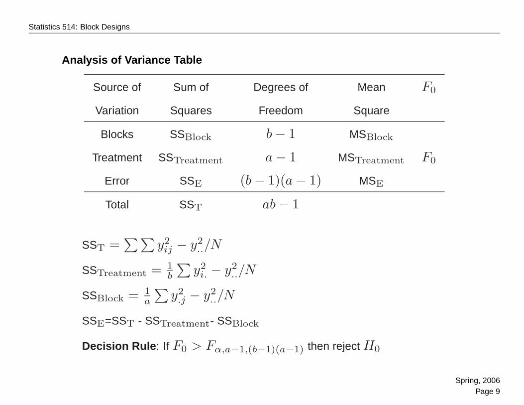
Analysis of Variance Table

Source of Sum of Degrees of Mean F0

Variation Squares Freedom Square

Blocks SSBlock b − 1 MSBlock

Treatment SSTreatment a − 1 MSTreatment F0

Error SSE (b − 1)(a − 1) MSE

Total SST ab − 1

SST =∑ ∑

y2ij − y2

../N

SSTreatment = 1b

∑y2

i. − y2../N

SSBlock = 1a

∑y2

.j − y2../N

SSE=SST - SSTreatment- SSBlock

Decision Rule : If F0 > Fα,a−1,(b−1)(a−1) then reject H0

Spring, 2006Page 9


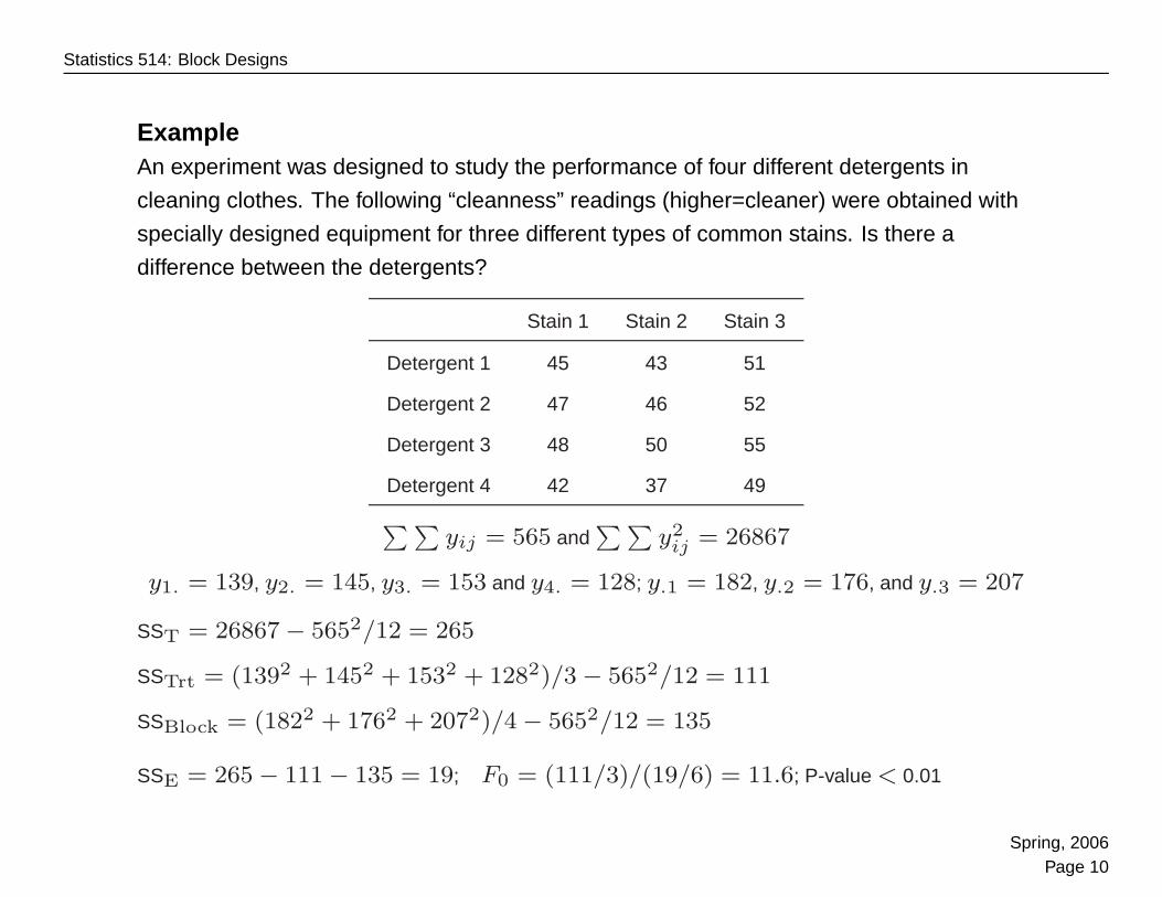
ExampleAn experiment was designed to study the performance of four different detergents in

cleaning clothes. The following “cleanness” readings (higher=cleaner) were obtained with

specially designed equipment for three different types of common stains. Is there a

difference between the detergents?

Stain 1 Stain 2 Stain 3

Detergent 1 45 43 51




∑ ∑yij = 565 and

∑ ∑y2

ij = 26867

y1. = 139, y2. = 145, y3. = 153 and y4. = 128; y.1 = 182, y.2 = 176, and y.3 = 207

SST = 26867 − 5652/12 = 265

SSTrt = (1392 + 1452 + 1532 + 1282)/3 − 5652/12 = 111

SSBlock = (1822 + 1762 + 2072)/4 − 5652/12 = 135

SSE = 265 − 111 − 135 = 19; F0 = (111/3)/(19/6) = 11.6; P-value < 0.01

Spring, 2006Page 10


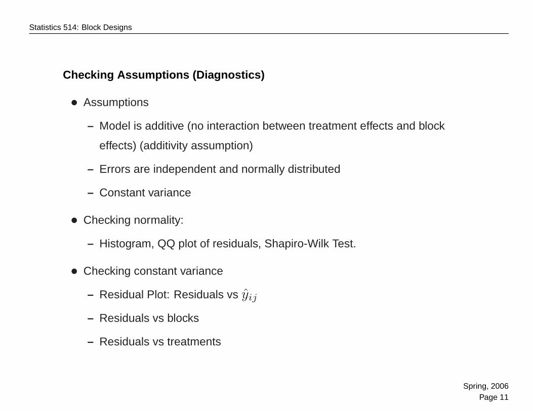
Checking Assumptions (Diagnostics)

• Assumptions

– Model is additive (no interaction between treatment effects and block

effects) (additivity assumption)

– Errors are independent and normally distributed

– Constant variance

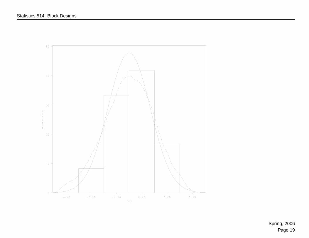
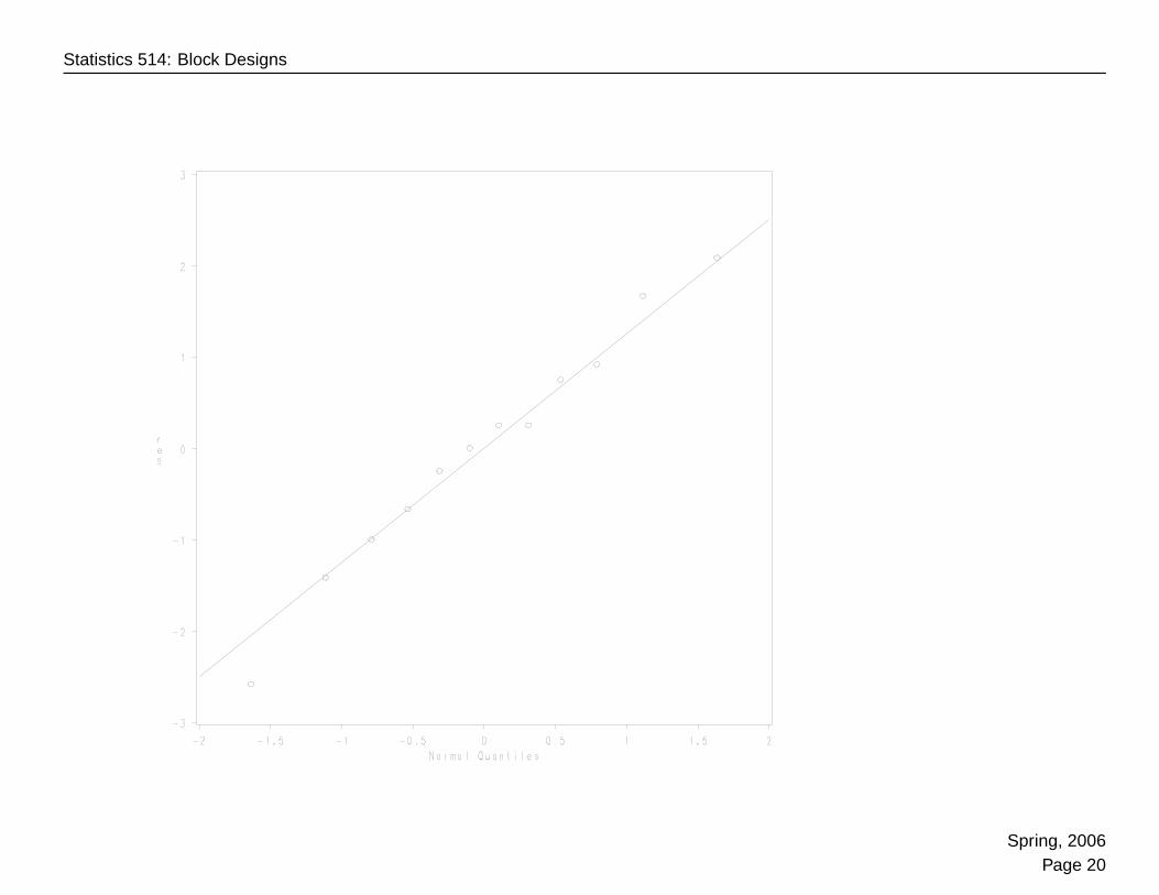
• Checking normality:

– Histogram, QQ plot of residuals, Shapiro-Wilk Test.

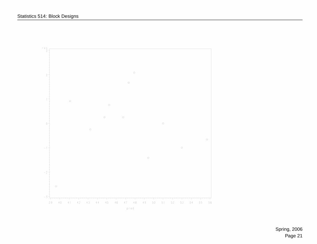
• Checking constant variance

– Residual Plot: Residuals vs yij

– Residuals vs blocks

– Residuals vs treatments

Spring, 2006Page 11


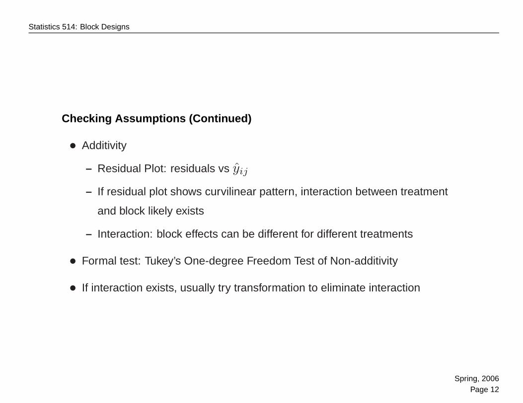
Checking Assumptions (Continued)

• Additivity

– Residual Plot: residuals vs yij

– If residual plot shows curvilinear pattern, interaction between treatment

and block likely exists

– Interaction: block effects can be different for different treatments

• Formal test: Tukey’s One-degree Freedom Test of Non-additivity

• If interaction exists, usually try transformation to eliminate interaction

Spring, 2006Page 12


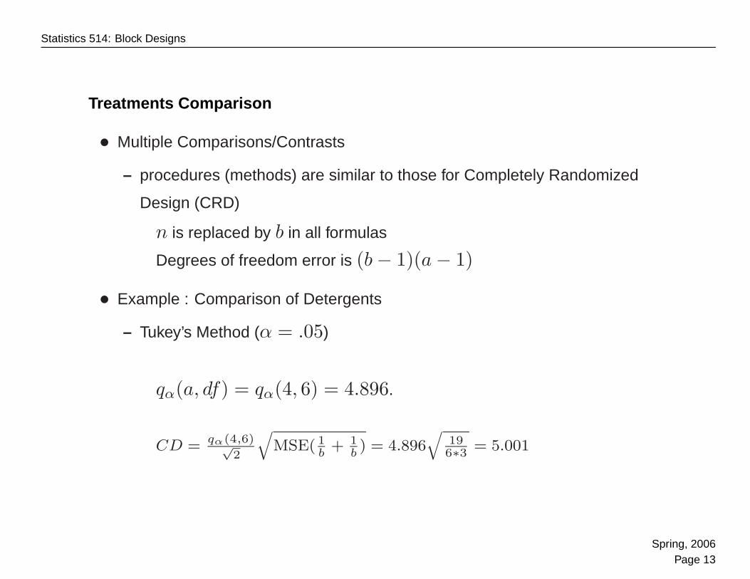
Treatments Comparison

• Multiple Comparisons/Contrasts

– procedures (methods) are similar to those for Completely Randomized

Design (CRD)

n is replaced by b in all formulas

Degrees of freedom error is (b − 1)(a − 1)

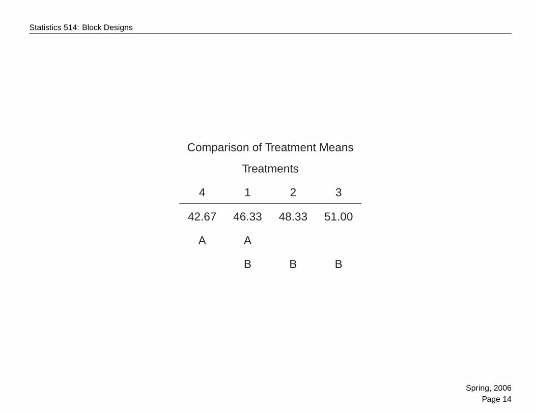
• Example : Comparison of Detergents

– Tukey’s Method (α = .05)

qα(a, df) = qα(4, 6) = 4.896.

CD =qα(4,6)√

2

√MSE( 1

b+ 1

b) = 4.896

√196∗3 = 5.001

Spring, 2006Page 13


Comparison of Treatment Means

Treatments

4 1 2 3

42.67 46.33 48.33 51.00

A A

B B B

Spring, 2006Page 14


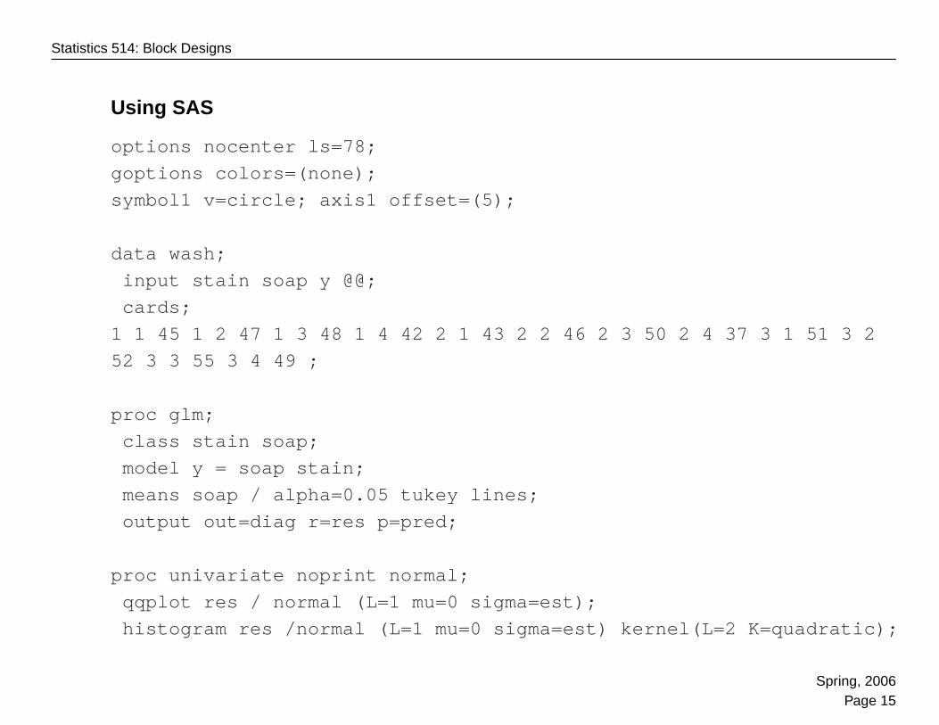
Using SAS

options nocenter ls=78;

goptions colors=(none);

symbol1 v=circle; axis1 offset=(5);

data wash;

input stain soap y @@;

cards;

1 1 45 1 2 47 1 3 48 1 4 42 2 1 43 2 2 46 2 3 50 2 4 37 3 1 51 3 2

52 3 3 55 3 4 49 ;

proc glm;

class stain soap;

model y = soap stain;

means soap / alpha=0.05 tukey lines;

output out=diag r=res p=pred;

proc univariate noprint normal;

qqplot res / normal (L=1 mu=0 sigma=est);

histogram res /normal (L=1 mu=0 sigma=est) kernel(L=2 K=quadratic);

Spring, 2006Page 15


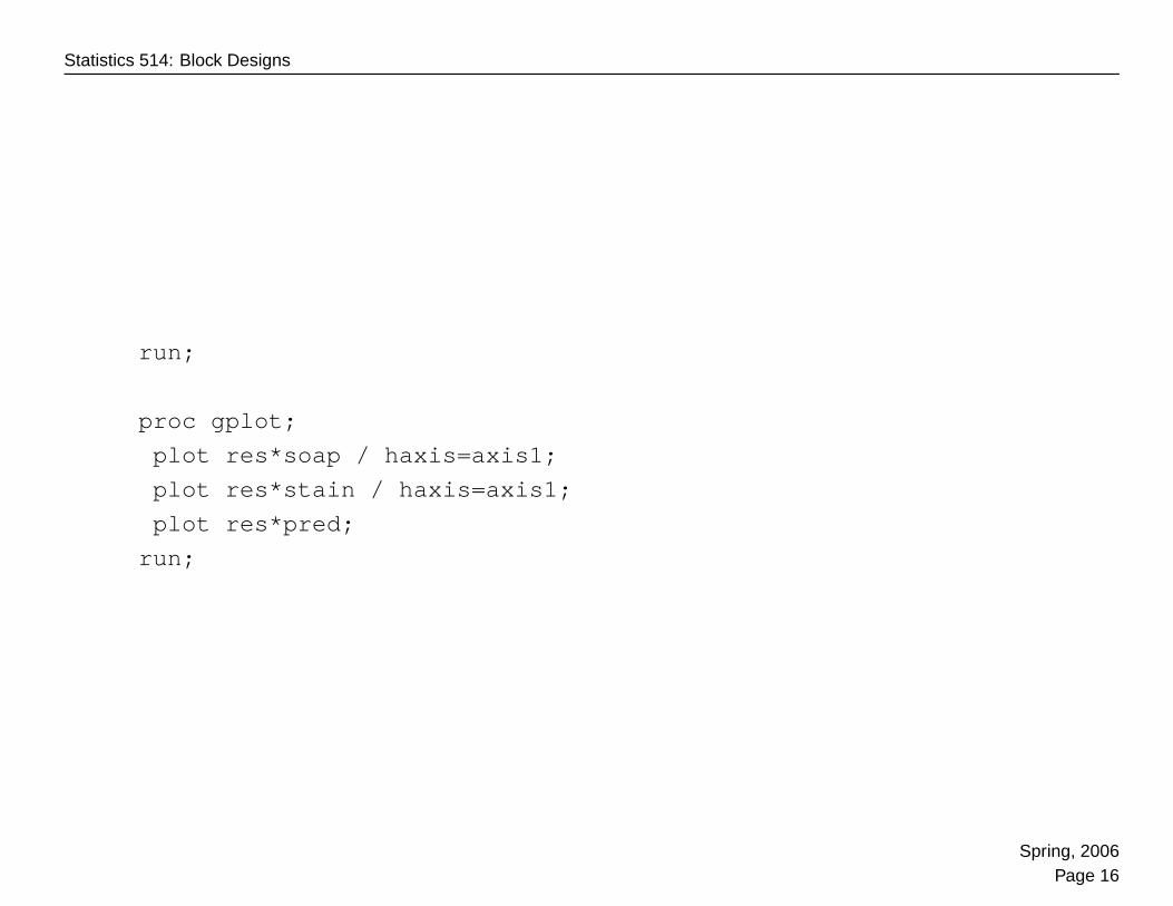
run;

proc gplot;

plot res*soap / haxis=axis1;

plot res*stain / haxis=axis1;

plot res*pred;

run;

Spring, 2006Page 16


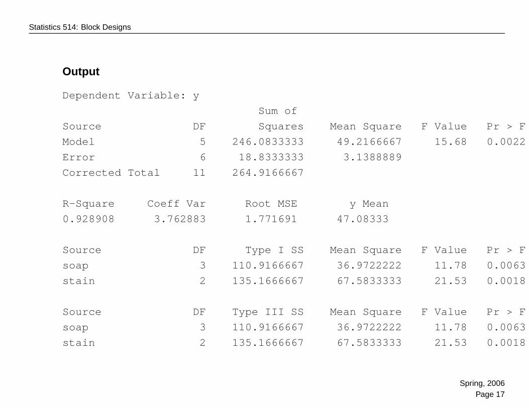
Output

Dependent Variable: y

Sum of

Source DF Squares Mean Square F Value Pr > F

Model 5 246.0833333 49.2166667 15.68 0.0022

Error 6 18.8333333 3.1388889

Corrected Total 11 264.9166667

R-Square Coeff Var Root MSE y Mean

0.928908 3.762883 1.771691 47.08333

Source DF Type I SS Mean Square F Value Pr > F

soap 3 110.9166667 36.9722222 11.78 0.0063

stain 2 135.1666667 67.5833333 21.53 0.0018

Source DF Type III SS Mean Square F Value Pr > F

soap 3 110.9166667 36.9722222 11.78 0.0063

stain 2 135.1666667 67.5833333 21.53 0.0018

Spring, 2006Page 17


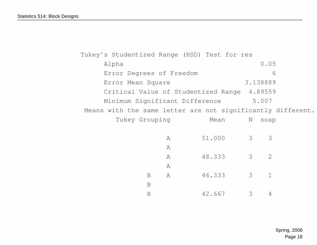
Tukey’s Studentized Range (HSD) Test for res

Alpha 0.05

Error Degrees of Freedom 6

Error Mean Square 3.138889

Critical Value of Studentized Range 4.89559

Minimum Significant Difference 5.007

Means with the same letter are not significantly different.

Tukey Grouping Mean N soap

A 51.000 3 3

A

A 48.333 3 2

A

B A 46.333 3 1

B

B 42.667 3 4

Spring, 2006Page 18


Spring, 2006Page 19


Spring, 2006Page 20


Spring, 2006Page 21


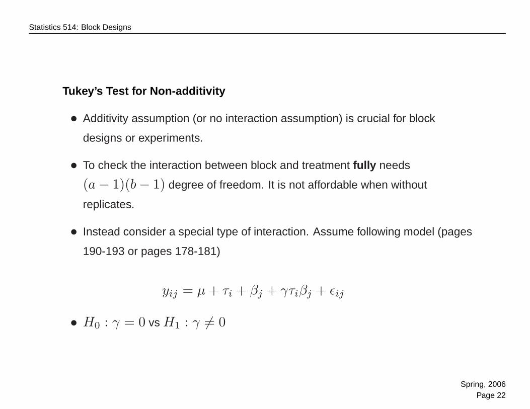
Tukey’s Test for Non-additivity

• Additivity assumption (or no interaction assumption) is crucial for block

designs or experiments.

• To check the interaction between block and treatment fully needs

(a − 1)(b − 1) degree of freedom. It is not affordable when without

replicates.

• Instead consider a special type of interaction. Assume following model (pages

190-193 or pages 178-181)

yij = µ + τi + βj + γτiβj + εij

• H0 : γ = 0 vs H1 : γ 6= 0

Spring, 2006Page 22


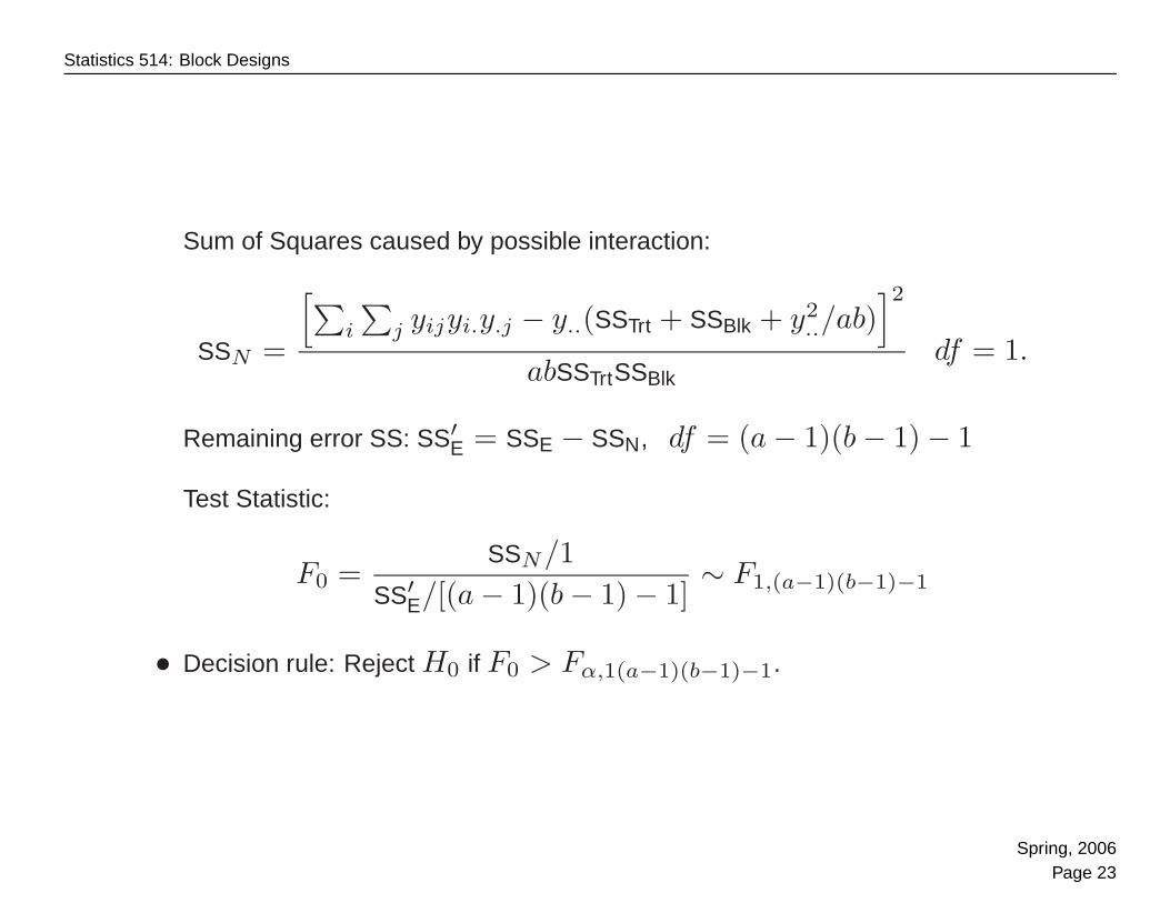
Sum of Squares caused by possible interaction:

SSN =

[∑i

∑j yijyi.y.j − y..(SSTrt + SSBlk + y2

../ab)]2

abSSTrtSSBlkdf = 1.

Remaining error SS: SS′E = SSE − SSN, df = (a − 1)(b − 1) − 1

Test Statistic:

F0 =SSN/1

SS′E/[(a − 1)(b − 1) − 1]

∼ F1,(a−1)(b−1)−1

• Decision rule: Reject H0 if F0 > Fα,1(a−1)(b−1)−1.

Spring, 2006Page 23


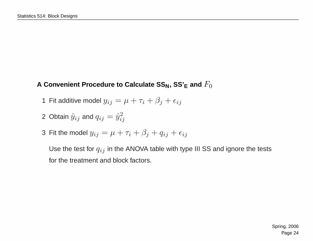
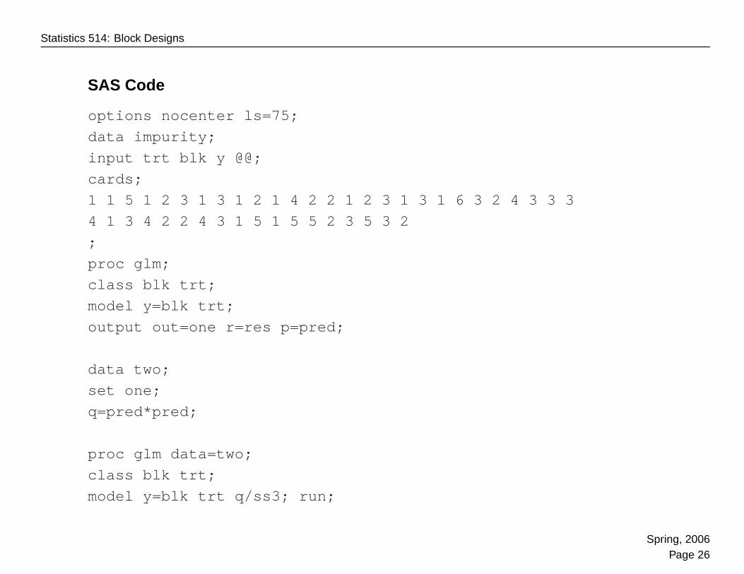
A Convenient Procedure to Calculate SS N, SS’E and F0

1 Fit additive model yij = µ + τi + βj + εij

2 Obtain yij and qij = y2ij

3 Fit the model yij = µ + τi + βj + qij + εij

Use the test for qij in the ANOVA table with type III SS and ignore the tests

for the treatment and block factors.

Spring, 2006Page 24


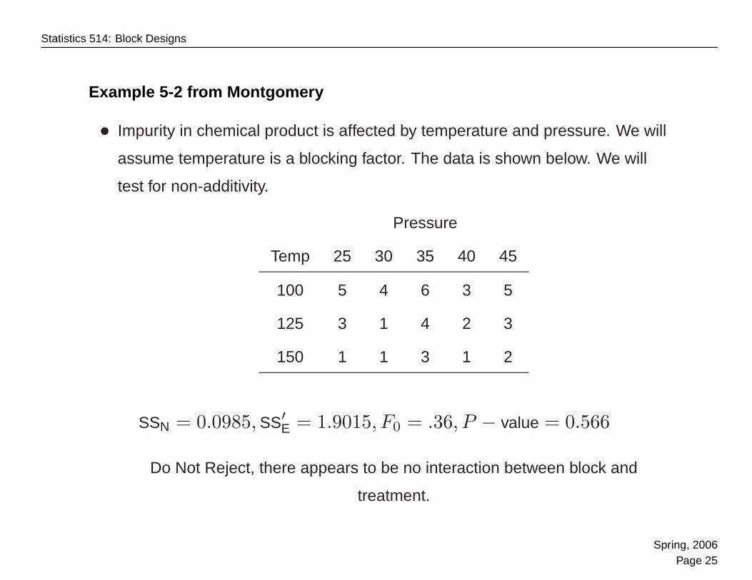
Example 5-2 from Montgomery

• Impurity in chemical product is affected by temperature and pressure. We will

assume temperature is a blocking factor. The data is shown below. We will

test for non-additivity.

Pressure

Temp 25 30 35 40 45

100 5 4 6 3 5

125 3 1 4 2 3

150 1 1 3 1 2

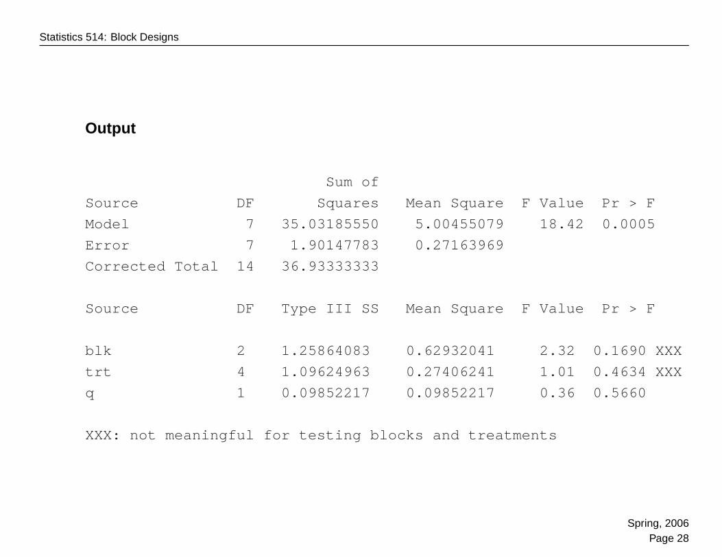
SSN = 0.0985, SS′E = 1.9015, F0 = .36, P − value = 0.566

Do Not Reject, there appears to be no interaction between block and

treatment.

Spring, 2006Page 25


SAS Code

options nocenter ls=75;

data impurity;

input trt blk y @@;

cards;

1 1 5 1 2 3 1 3 1 2 1 4 2 2 1 2 3 1 3 1 6 3 2 4 3 3 3

4 1 3 4 2 2 4 3 1 5 1 5 5 2 3 5 3 2

;

proc glm;

class blk trt;

model y=blk trt;

output out=one r=res p=pred;

data two;

set one;

q=pred*pred;

proc glm data=two;

class blk trt;

model y=blk trt q/ss3; run;

Spring, 2006Page 26


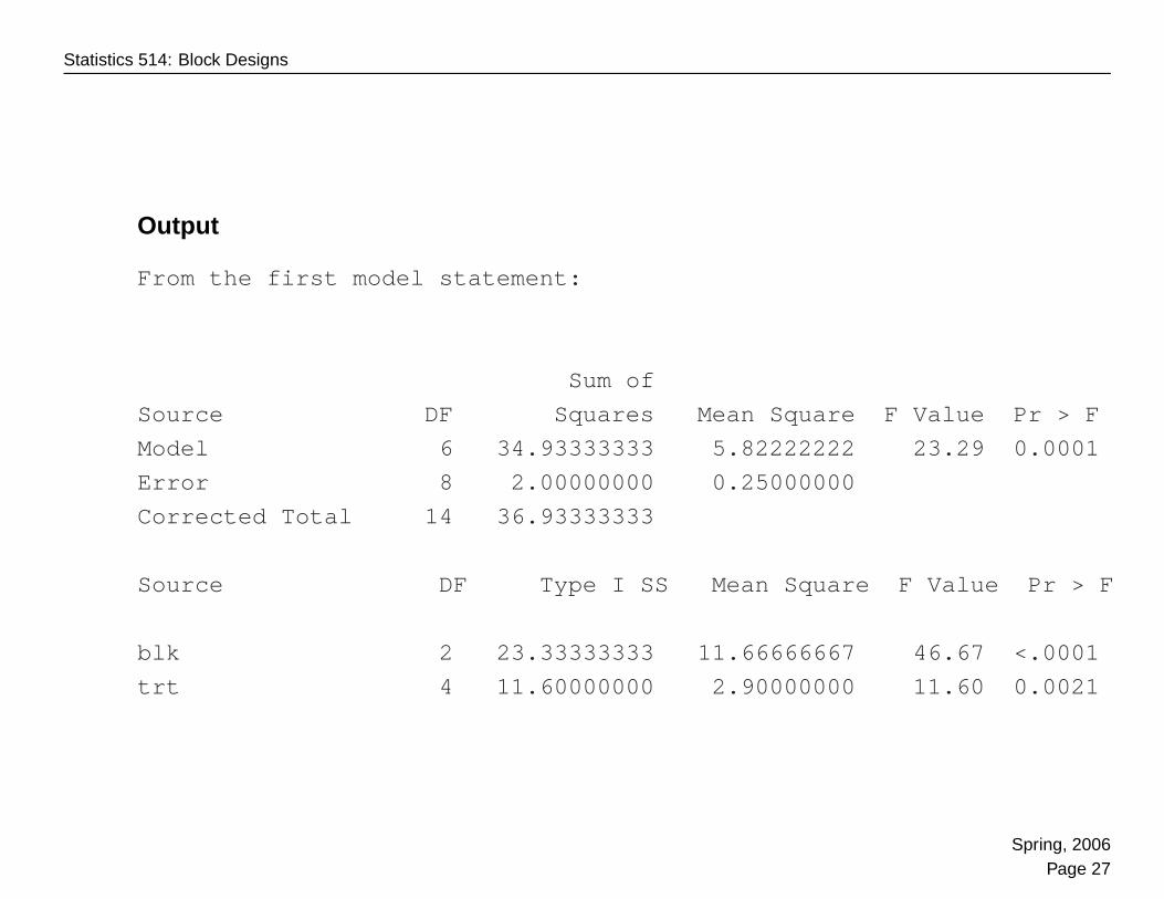
Output

From the first model statement:

Sum of


Model 6 34.93333333 5.82222222 23.29 0.0001

Error 8 2.00000000 0.25000000


Source DF Type I SS Mean Square F Value Pr > F

blk 2 23.33333333 11.66666667 46.67 <.0001

trt 4 11.60000000 2.90000000 11.60 0.0021

Spring, 2006Page 27


Output

Sum of


Model 7 35.03185550 5.00455079 18.42 0.0005

Error 7 1.90147783 0.27163969


Source DF Type III SS Mean Square F Value Pr > F

blk 2 1.25864083 0.62932041 2.32 0.1690 XXX

trt 4 1.09624963 0.27406241 1.01 0.4634 XXX

q 1 0.09852217 0.09852217 0.36 0.5660

XXX: not meaningful for testing blocks and treatments

Spring, 2006Page 28


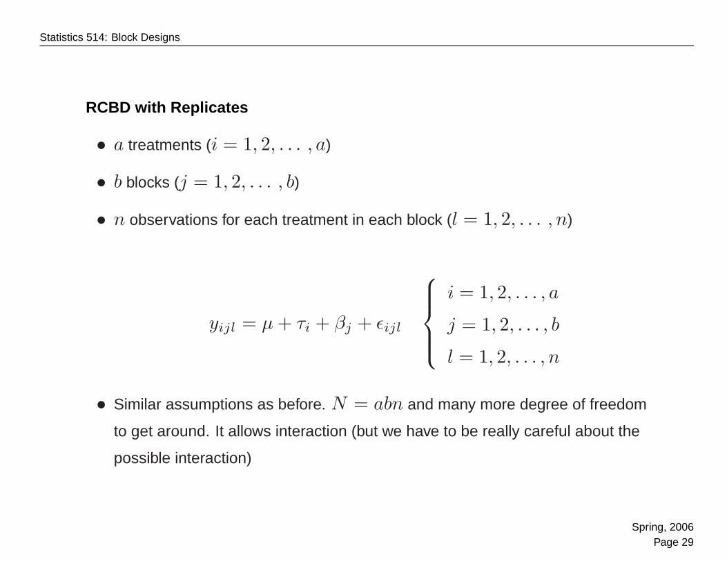
RCBD with Replicates

• a treatments (i = 1, 2, . . . , a)

• b blocks (j = 1, 2, . . . , b)

• n observations for each treatment in each block (l = 1, 2, . . . , n)

yijl = µ + τi + βj + εijl

i = 1, 2, . . . , a

j = 1, 2, . . . , b

l = 1, 2, . . . , n

• Similar assumptions as before. N = abn and many more degree of freedom

to get around. It allows interaction (but we have to be really careful about the

possible interaction)

Spring, 2006Page 29


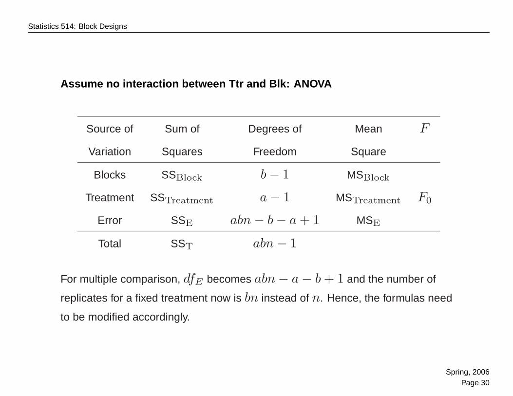
Assume no interaction between Ttr and Blk: ANOVA

Source of Sum of Degrees of Mean F




Error SSE abn − b − a + 1 MSE

Total SST abn − 1

For multiple comparison, dfE becomes abn − a − b + 1 and the number of

replicates for a fixed treatment now is bn instead of n. Hence, the formulas need

to be modified accordingly.

Spring, 2006Page 30


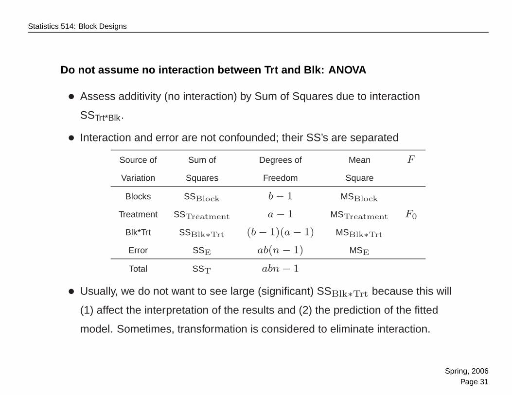
Do not assume no interaction between Trt and Blk: ANOVA

• Assess additivity (no interaction) by Sum of Squares due to interaction

SSTrt*Blk.

• Interaction and error are not confounded; their SS’s are separated

Source of Sum of Degrees of Mean F




Blk*Trt SSBlk∗Trt (b − 1)(a − 1) MSBlk∗Trt

Error SSE ab(n − 1) MSE

Total SST abn − 1

• Usually, we do not want to see large (significant) SSBlk∗Trt because this will

(1) affect the interpretation of the results and (2) the prediction of the fitted

model. Sometimes, transformation is considered to eliminate interaction.

Spring, 2006Page 31

Documents

Montgomery: Chapter 4 Lecture 6: Block Designsyuzhu/stat514s2006/Lecnot/blockdesigns2006... · Lecture 6: Block Designs Montgomery: Chapter 4 Spring, 2006 Page 1. Statistics 514: