Embed Size (px)
Citation preview
ANALYSIS & DESIGN OF LAZY-WAVE STEEL CATENARY RISERS
MSc. Subsea Engineering
Class Code NM958/NM521
Alexandros Venetsanos Reg.No 201459239 Scholar of Hellenic Petroleum S.A.
Scholar of Foundation of Education & European Culture
Angelos Papavasileiou Reg.No 201490748
Lecturer Dr. N.Srinil
Glasgow 2014
Analysis & Design of LWSCR & SCR
1 A.Venetsanos, A.Papavasileiou
INTRODUCTION
The main objective of this study is the investigation of the design parameters which affect the shape and the static loading of LWR. For this purpose, the catenary theory was applied. In addition, a Matlab code was developed for the evaluation of different scenarios. Furthermore, special cases where the LWR configuration degenerates into “Shaped” or “Steep Wave” SCR were examined. Finally, the influence of the hang-off point deflection in the geometry and the loads of the riser was taken into consideration.
Chapter 1 – Theory
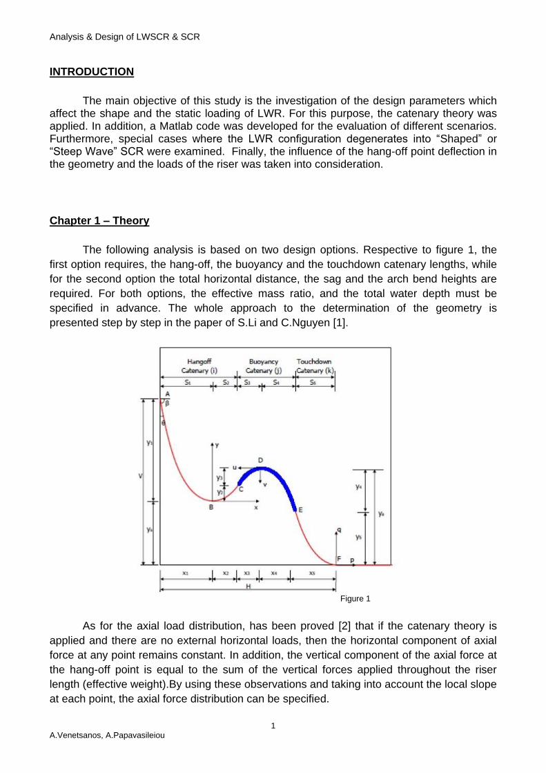
The following analysis is based on two design options. Respective to figure 1, the
first option requires, the hang-off, the buoyancy and the touchdown catenary lengths, while
for the second option the total horizontal distance, the sag and the arch bend heights are
required. For both options, the effective mass ratio, and the total water depth must be
specified in advance. The whole approach to the determination of the geometry is
presented step by step in the paper of S.Li and C.Nguyen [1].
Figure 1
As for the axial load distribution, has been proved [2] that if the catenary theory is
applied and there are no external horizontal loads, then the horizontal component of axial
force at any point remains constant. In addition, the vertical component of the axial force at
the hang-off point is equal to the sum of the vertical forces applied throughout the riser
length (effective weight).By using these observations and taking into account the local slope
at each point, the axial force distribution can be specified.
Analysis & Design of LWSCR & SCR
2 A.Venetsanos, A.Papavasileiou
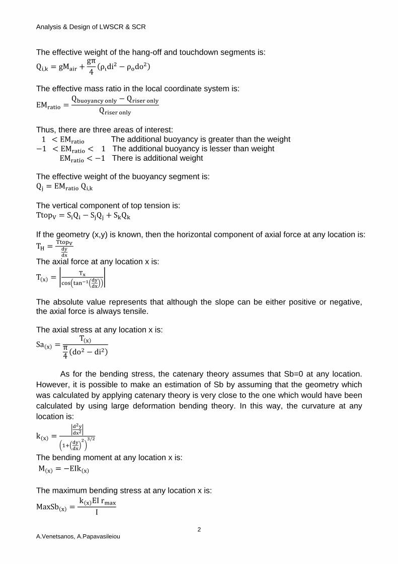
The effective weight of the hang-off and touchdown segments is:
Qi,k = gMair +gπ
4(ριdi2 − ροdo2)
The effective mass ratio in the local coordinate system is:
EMratio =Qbuoyancy only − Qriser only
Qriser only
Thus, there are three areas of interest:
1 < EMratio The additional buoyancy is greater than the weight −1 < EMratio < 1 The additional buoyancy is lesser than weight
EMratio < −1 There is additional weight The effective weight of the buoyancy segment is: Qj = EMratio Qi,k
The vertical component of top tension is: TtopV = SiQi − SjQj + SkQk
If the geometry (x,y) is known, then the horizontal component of axial force at any location is:
TH =TtopV
dy
dx
The axial force at any location x is:
T(x) = |Tx
cos(tan−1(dy
dx))
|
The absolute value represents that although the slope can be either positive or negative, the axial force is always tensile. The axial stress at any location x is:
Sa(x) =T(x)
π4
(do2 − di2)
As for the bending stress, the catenary theory assumes that Sb=0 at any location.
However, it is possible to make an estimation of Sb by assuming that the geometry which
was calculated by applying catenary theory is very close to the one which would have been
calculated by using large deformation bending theory. In this way, the curvature at any
location is:
k(x) =|d2y
dx2|
(1+(dy
dx)
2)
3/2
The bending moment at any location x is:
M(x) = −EIk(x)
The maximum bending stress at any location x is:
MaxSb(x) = k(x)EI rmax
I
Analysis & Design of LWSCR & SCR
3 A.Venetsanos, A.Papavasileiou
The above calculations require the first and the second difference (dy
dx ,
d2y
dx2). For this
purpose, there are two alternative approaches. The first is analytical and has to be applied
in each local coordinate system individually. The second is numerical and has to be applied
to the global coordinate system. On the one hand, the first method is most accurate.
However, it may not work correctly at points of discontinuity. On the other side, the
accuracy of the second method depends on the number of points and could ignore
discontinuities. In this study, the numerical approximation was adopted, and the total length
was divided into 10000 parts. The finite difference formulas are given below [3].
Forward difference approximation
dy
dx|
xi
≈−y(xi+2)+4y(xi+1)−3y(xi)
2h
d2y
dx2|
xi
≈y(xi+2) − 2y(xi+1) + y(xi)
h2
Backward difference approximation
dy
dx|
xi
≈3y(xi) − 4y(xi−1) + y(xi−2)
2h
d2y
dx2|
xi
≈y(xi) − 2y(xi−1) + y(xi−2)
h2
Central difference approximation
dy
dx|
xi
≈−y(xi+2) + 8y(xi+1) − 8y(xi−1) + y(xi−2)
12h
d2y
dx2|xi
≈y(xi+1)−2y(xi)+y(xi−1)
h2 (This formula was not used in this study for simplicity.)
As far as catenary theory does not take into account the shear stress, the total
maximum stress at any location is the sum of axial stress and maximum bending stress.
MaxStotal(x) = Sa(x) + MaxSb(x)
Analysis & Design of LWSCR & SCR
4 A.Venetsanos, A.Papavasileiou
Figure 2
Figure 3
Analysis & Design of LWSCR & SCR
5 A.Venetsanos, A.Papavasileiou
Figure 4
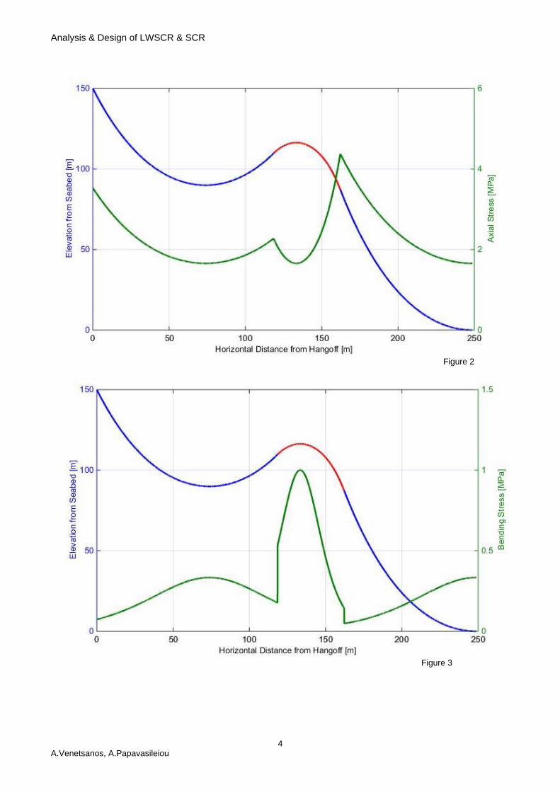
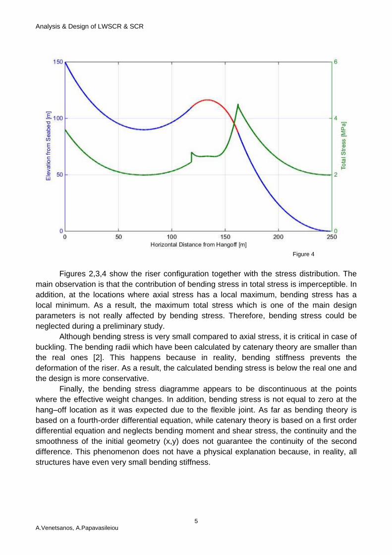
Figures 2,3,4 show the riser configuration together with the stress distribution. The
main observation is that the contribution of bending stress in total stress is imperceptible. In
addition, at the locations where axial stress has a local maximum, bending stress has a
local minimum. As a result, the maximum total stress which is one of the main design
parameters is not really affected by bending stress. Therefore, bending stress could be
neglected during a preliminary study.
Although bending stress is very small compared to axial stress, it is critical in case of
buckling. The bending radii which have been calculated by catenary theory are smaller than
the real ones [2]. This happens because in reality, bending stiffness prevents the
deformation of the riser. As a result, the calculated bending stress is below the real one and
the design is more conservative.
Finally, the bending stress diagramme appears to be discontinuous at the points
where the effective weight changes. In addition, bending stress is not equal to zero at the
hang–off location as it was expected due to the flexible joint. As far as bending theory is
based on a fourth-order differential equation, while catenary theory is based on a first order
differential equation and neglects bending moment and shear stress, the continuity and the
smoothness of the initial geometry (x,y) does not guarantee the continuity of the second
difference. This phenomenon does not have a physical explanation because, in reality, all
structures have even very small bending stiffness.
Analysis & Design of LWSCR & SCR
6 A.Venetsanos, A.Papavasileiou
Chapter 2 – Matlab Code
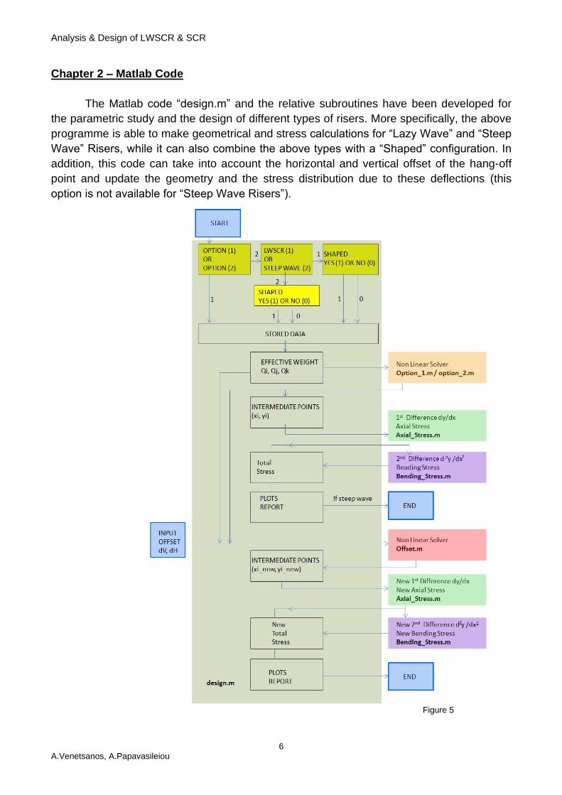
The Matlab code “design.m” and the relative subroutines have been developed for
the parametric study and the design of different types of risers. More specifically, the above
programme is able to make geometrical and stress calculations for “Lazy Wave” and “Steep
Wave” Risers, while it can also combine the above types with a “Shaped” configuration. In
addition, this code can take into account the horizontal and vertical offset of the hang-off
point and update the geometry and the stress distribution due to these deflections (this
option is not available for “Steep Wave Risers”).
Figure 5
Analysis & Design of LWSCR & SCR
7 A.Venetsanos, A.Papavasileiou
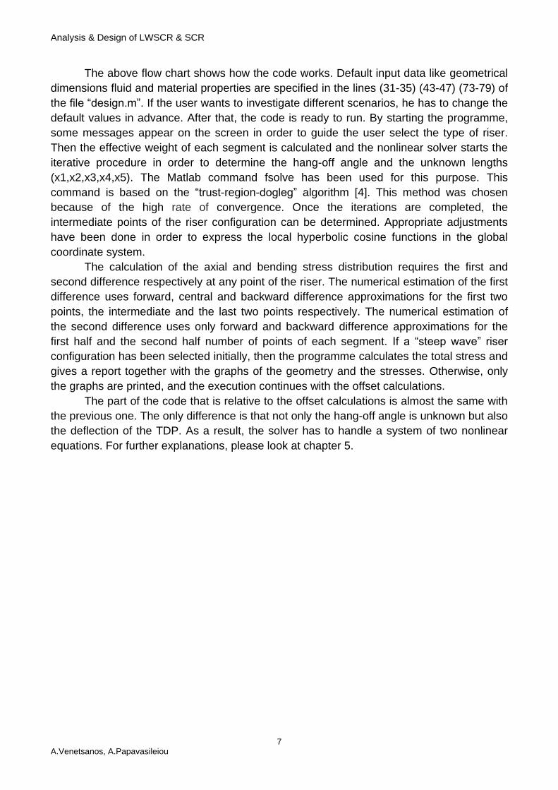
The above flow chart shows how the code works. Default input data like geometrical
dimensions fluid and material properties are specified in the lines (31-35) (43-47) (73-79) of
the file “design.m”. If the user wants to investigate different scenarios, he has to change the
default values in advance. After that, the code is ready to run. By starting the programme,
some messages appear on the screen in order to guide the user select the type of riser.
Then the effective weight of each segment is calculated and the nonlinear solver starts the
iterative procedure in order to determine the hang-off angle and the unknown lengths
(x1,x2,x3,x4,x5). The Matlab command fsolve has been used for this purpose. This
command is based on the “trust-region-dogleg” algorithm [4]. This method was chosen
because of the high rate of convergence. Once the iterations are completed, the
intermediate points of the riser configuration can be determined. Appropriate adjustments
have been done in order to express the local hyperbolic cosine functions in the global
coordinate system.
The calculation of the axial and bending stress distribution requires the first and
second difference respectively at any point of the riser. The numerical estimation of the first
difference uses forward, central and backward difference approximations for the first two
points, the intermediate and the last two points respectively. The numerical estimation of
the second difference uses only forward and backward difference approximations for the
first half and the second half number of points of each segment. If a “steep wave” riser
configuration has been selected initially, then the programme calculates the total stress and
gives a report together with the graphs of the geometry and the stresses. Otherwise, only
the graphs are printed, and the execution continues with the offset calculations.
The part of the code that is relative to the offset calculations is almost the same with
the previous one. The only difference is that not only the hang-off angle is unknown but also
the deflection of the TDP. As a result, the solver has to handle a system of two nonlinear
equations. For further explanations, please look at chapter 5.
Analysis & Design of LWSCR & SCR
8 A.Venetsanos, A.Papavasileiou
Chapter 3 – Effect of Pipe Size & Fluids Properties
This chapter deals with the effect of pipe size and fluids properties (internal &
external) on the geometry and the maximum stress of the riser. Four different scenarios
were investigated. The lengths Si, Sj, Sk, the water depth and the effective mass ratio
remain steady in any case. As for the rest properties, in each scenario only one parameter
changes in order to highlight how this parameter influences the overall design. The only
exception is the first scenario where two different flexible pipes were examined.
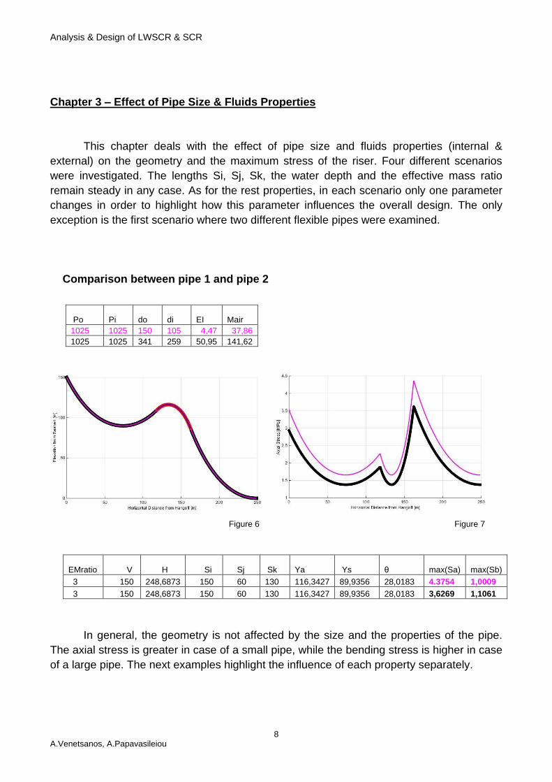
Comparison between pipe 1 and pipe 2
Figure 6 Figure 7
EMratio V H Si Sj Sk Ya Ys θ max(Sa) max(Sb)
3 150 248,6873 150 60 130 116,3427 89,9356 28,0183 4.3754 1,0009
3 150 248,6873 150 60 130 116,3427 89,9356 28,0183 3,6269 1,1061
In general, the geometry is not affected by the size and the properties of the pipe.
The axial stress is greater in case of a small pipe, while the bending stress is higher in case
of a large pipe. The next examples highlight the influence of each property separately.
Po Pi do di EI Mair
1025 1025 150 105 4,47 37,86
1025 1025 341 259 50,95 141,62
Analysis & Design of LWSCR & SCR
9 A.Venetsanos, A.Papavasileiou
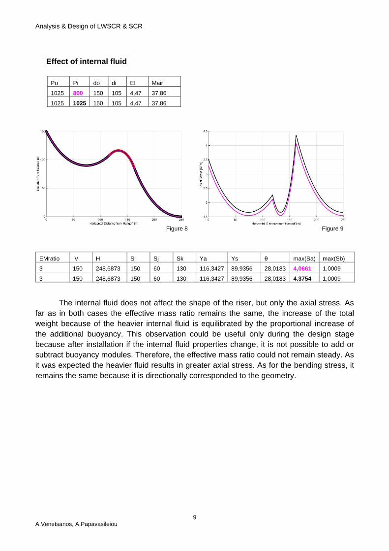
Effect of internal fluid
Figure 8 Figure 9
The internal fluid does not affect the shape of the riser, but only the axial stress. As
far as in both cases the effective mass ratio remains the same, the increase of the total
weight because of the heavier internal fluid is equilibrated by the proportional increase of
the additional buoyancy. This observation could be useful only during the design stage
because after installation if the internal fluid properties change, it is not possible to add or
subtract buoyancy modules. Therefore, the effective mass ratio could not remain steady. As
it was expected the heavier fluid results in greater axial stress. As for the bending stress, it
remains the same because it is directionally corresponded to the geometry.
Po Pi do di EI Mair
1025 800 150 105 4,47 37,86
1025 1025 150 105 4,47 37,86
EMratio V H Si Sj Sk Ya Ys θ max(Sa) max(Sb)
3 150 248,6873 150 60 130 116,3427 89,9356 28,0183 4,0661 1,0009
3 150 248,6873 150 60 130 116,3427 89,9356 28,0183 4.3754 1,0009
Analysis & Design of LWSCR & SCR
10 A.Venetsanos, A.Papavasileiou
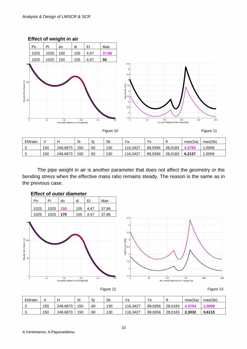
Effect of weight in air
Po Pi do di EI Mair 1025 1025 150 105 4,47 37,86 1025 1025 150 105 4,47 50
Figure 10 Figure 11
EMratio V H Si Sj Sk Ya Ys θ max(Sa) max(Sb)
3 150 248,6873 150 60 130 116,3427 89,9356 28,0183 4.3754 1,0009
3 150 248,6873 150 60 130 116,3427 89,9356 28,0183 6,2137 1,0009
The pipe weight in air is another parameter that does not affect the geometry or the
bending stress when the effective mass ratio remains steady. The reason is the same as in
the previous case.
Effect of outer diameter
Po Pi do di EI Mair
1025 1025 150 105 4,47 37,86
1025 1025 170 105 4,47 37,86
Figure 12 Figure 13
EMratio V H Si Sj Sk Ya Ys θ max(Sa) max(Sb)
3 150 248,6873 150 60 130 116,3427 89,9356 28,0183 4.3754 1,0009
3 150 248,6873 150 60 130 116,3427 89,9356 28,0183 2,3032 0,6115
Analysis & Design of LWSCR & SCR
11 A.Venetsanos, A.Papavasileiou
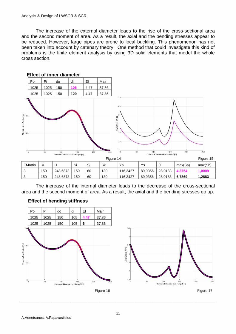
The increase of the external diameter leads to the rise of the cross-sectional area and the second moment of area. As a result, the axial and the bending stresses appear to be reduced. However, large pipes are prone to local buckling. This phenomenon has not been taken into account by catenary theory. One method that could investigate this kind of problems is the finite element analysis by using 3D solid elements that model the whole cross section. Effect of inner diameter
Po Pi do di EI Mair
1025 1025 150 105 4,47 37,86
1025 1025 150 120 4,47 37,86
Figure 14 Figure 15
EMratio V H Si Sj Sk Ya Ys θ max(Sa) max(Sb)
3 150 248,6873 150 60 130 116,3427 89,9356 28,0183 4.3754 1,0009
3 150 248,6873 150 60 130 116,3427 89,9356 28,0183 6,7869 1,2883
The increase of the internal diameter leads to the decrease of the cross-sectional
area and the second moment of area. As a result, the axial and the bending stresses go up.
Effect of bending stiffness
Po Pi do di EI Mair
1025 1025 150 105 4,47 37,86
1025 1025 150 105 6 37,86
Figure 16 Figure 17
Analysis & Design of LWSCR & SCR
12 A.Venetsanos, A.Papavasileiou
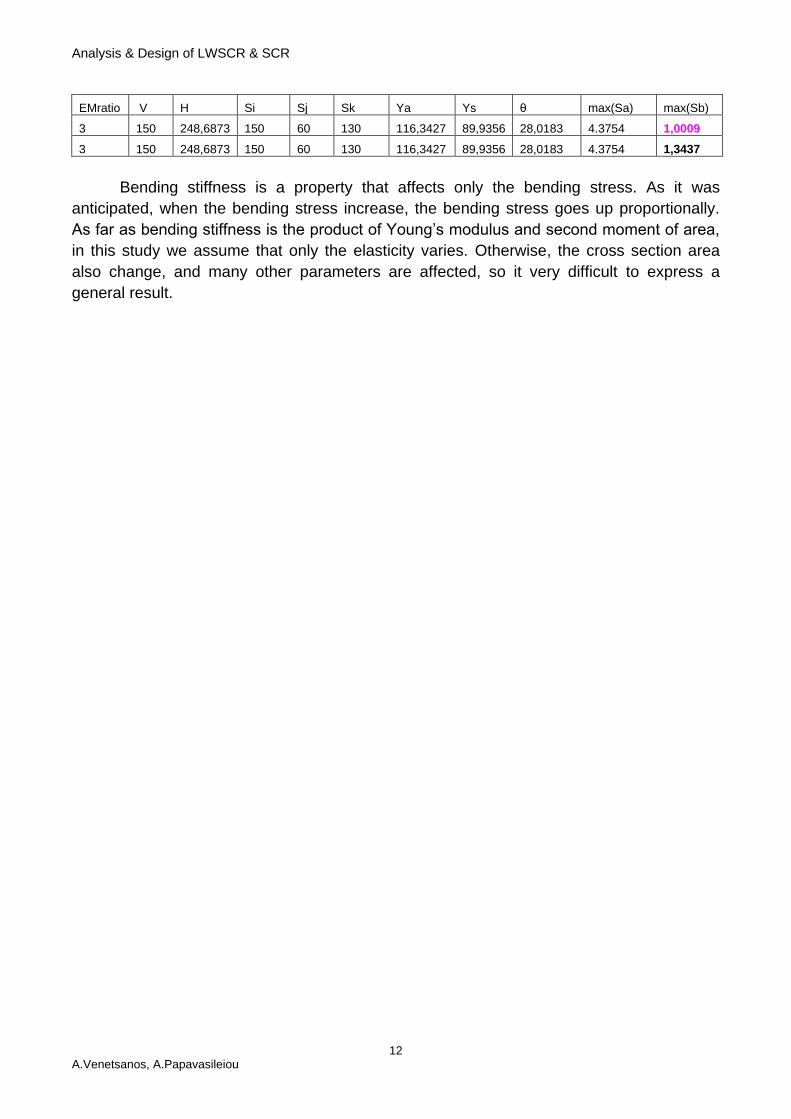
EMratio V H Si Sj Sk Ya Ys θ max(Sa) max(Sb)
3 150 248,6873 150 60 130 116,3427 89,9356 28,0183 4.3754 1,0009
3 150 248,6873 150 60 130 116,3427 89,9356 28,0183 4.3754 1,3437
Bending stiffness is a property that affects only the bending stress. As it was
anticipated, when the bending stress increase, the bending stress goes up proportionally.
As far as bending stiffness is the product of Young’s modulus and second moment of area,
in this study we assume that only the elasticity varies. Otherwise, the cross section area
also change, and many other parameters are affected, so it very difficult to express a
general result.
Analysis & Design of LWSCR & SCR
13 A.Venetsanos, A.Papavasileiou
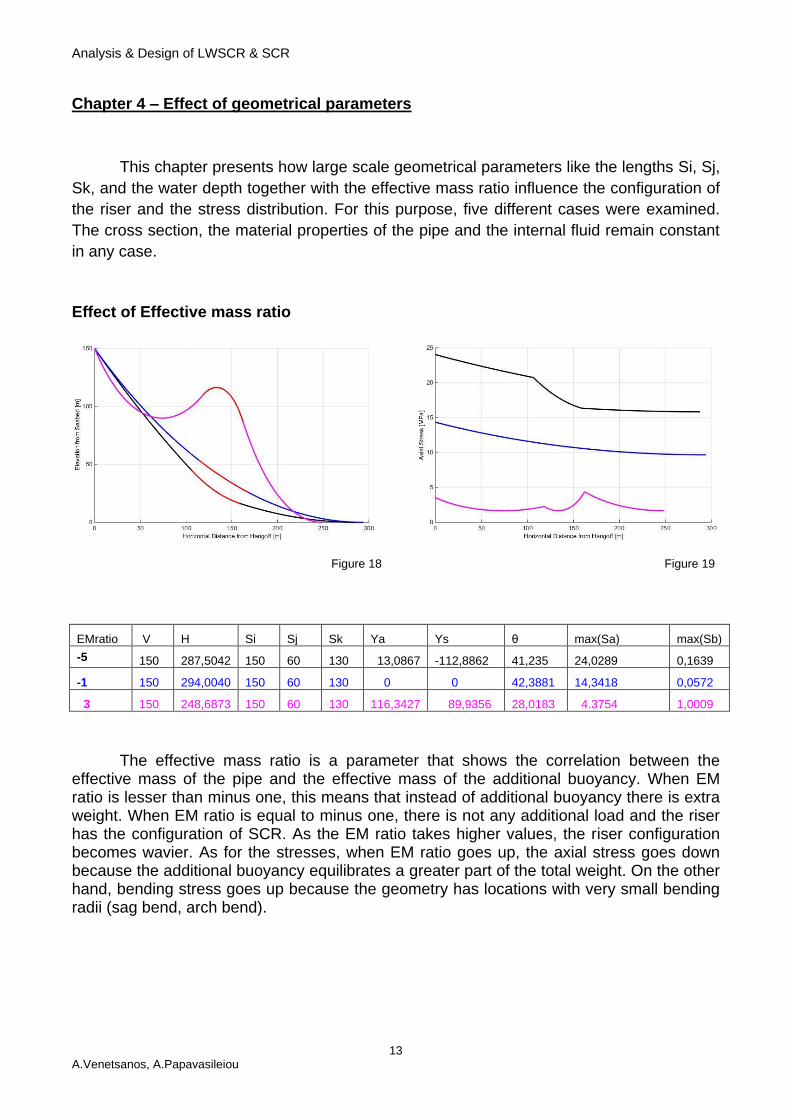
Chapter 4 – Effect of geometrical parameters
This chapter presents how large scale geometrical parameters like the lengths Si, Sj,
Sk, and the water depth together with the effective mass ratio influence the configuration of
the riser and the stress distribution. For this purpose, five different cases were examined.
The cross section, the material properties of the pipe and the internal fluid remain constant
in any case.
Effect of Effective mass ratio
Figure 18 Figure 19
The effective mass ratio is a parameter that shows the correlation between the
effective mass of the pipe and the effective mass of the additional buoyancy. When EM ratio is lesser than minus one, this means that instead of additional buoyancy there is extra weight. When EM ratio is equal to minus one, there is not any additional load and the riser has the configuration of SCR. As the EM ratio takes higher values, the riser configuration becomes wavier. As for the stresses, when EM ratio goes up, the axial stress goes down because the additional buoyancy equilibrates a greater part of the total weight. On the other hand, bending stress goes up because the geometry has locations with very small bending radii (sag bend, arch bend).
EMratio V H Si Sj Sk Ya Ys θ max(Sa) max(Sb)
-5 150 287,5042 150 60 130 13,0867 -112,8862 41,235 24,0289 0,1639
-1 150 294,0040 150 60 130 0 0 42,3881 14,3418 0,0572
3 150 248,6873 150 60 130 116,3427 89,9356 28,0183 4.3754 1,0009
Analysis & Design of LWSCR & SCR
14 A.Venetsanos, A.Papavasileiou
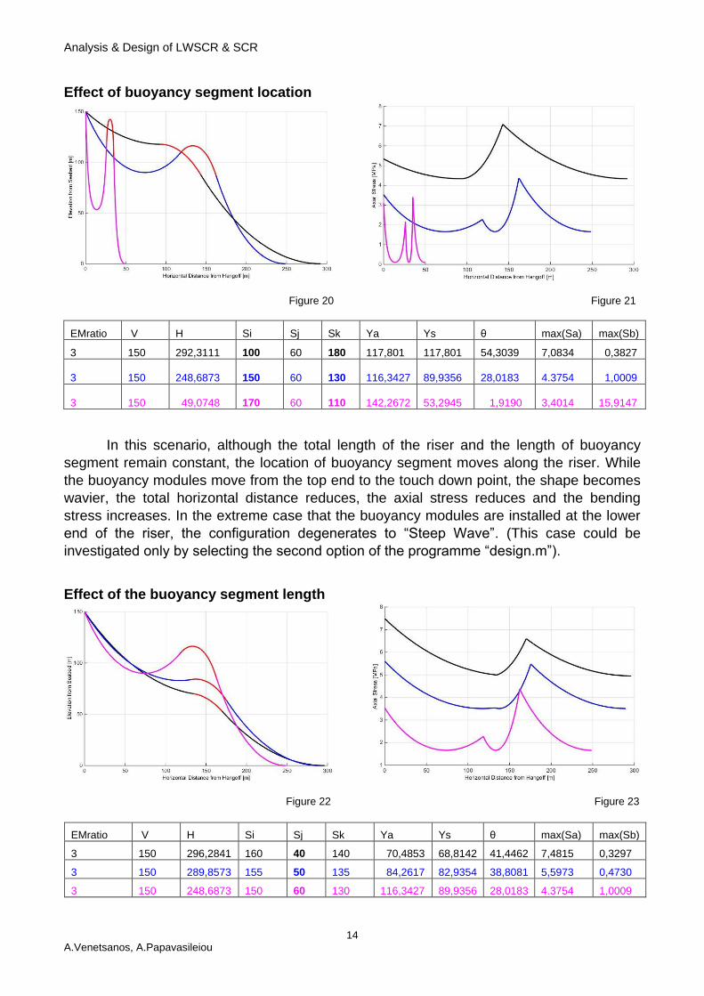
Effect of buoyancy segment location
Figure 20 Figure 21
EMratio V H Si Sj Sk Ya Ys θ max(Sa) max(Sb)
3 150 292,3111 100 60 180 117,801 117,801 54,3039 7,0834 0,3827
3 150 248,6873 150 60 130 116,3427 89,9356 28,0183 4.3754 1,0009
3 150 49,0748 170 60 110 142,2672 53,2945 1,9190 3,4014 15,9147
In this scenario, although the total length of the riser and the length of buoyancy
segment remain constant, the location of buoyancy segment moves along the riser. While
the buoyancy modules move from the top end to the touch down point, the shape becomes
wavier, the total horizontal distance reduces, the axial stress reduces and the bending
stress increases. In the extreme case that the buoyancy modules are installed at the lower
end of the riser, the configuration degenerates to “Steep Wave”. (This case could be
investigated only by selecting the second option of the programme “design.m”).
Effect of the buoyancy segment length
Figure 22 Figure 23
EMratio V H Si Sj Sk Ya Ys θ max(Sa) max(Sb)
3 150 296,2841 160 40 140 70,4853 68,8142 41,4462 7,4815 0,3297
3 150 289,8573 155 50 135 84,2617 82,9354 38,8081 5,5973 0,4730
3 150 248,6873 150 60 130 116,3427 89,9356 28,0183 4.3754 1,0009
Analysis & Design of LWSCR & SCR
15 A.Venetsanos, A.Papavasileiou
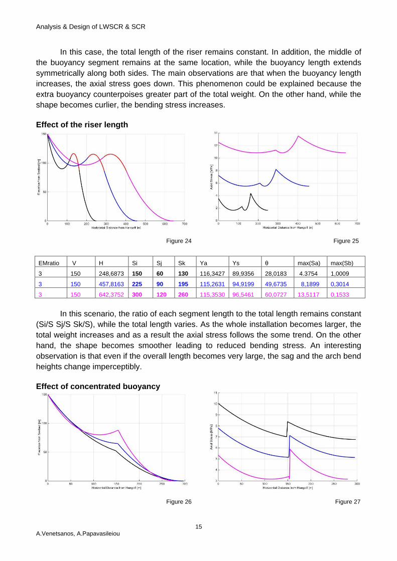
In this case, the total length of the riser remains constant. In addition, the middle of
the buoyancy segment remains at the same location, while the buoyancy length extends
symmetrically along both sides. The main observations are that when the buoyancy length
increases, the axial stress goes down. This phenomenon could be explained because the
extra buoyancy counterpoises greater part of the total weight. On the other hand, while the
shape becomes curlier, the bending stress increases.
Effect of the riser length
Figure 24 Figure 25
In this scenario, the ratio of each segment length to the total length remains constant
(Si/S Sj/S Sk/S), while the total length varies. As the whole installation becomes larger, the
total weight increases and as a result the axial stress follows the some trend. On the other
hand, the shape becomes smoother leading to reduced bending stress. An interesting
observation is that even if the overall length becomes very large, the sag and the arch bend
heights change imperceptibly.
Effect of concentrated buoyancy
Figure 26 Figure 27
EMratio V H Si Sj Sk Ya Ys θ max(Sa) max(Sb)
3 150 248,6873 150 60 130 116,3427 89,9356 28,0183 4.3754 1,0009
3 150 457,8163 225 90 195 115,2631 94,9199 49,6735 8,1899 0,3014
3 150 642,3752 300 120 260 115,3530 96,5461 60,0727 13,5117 0,1533
Analysis & Design of LWSCR & SCR
16 A.Venetsanos, A.Papavasileiou
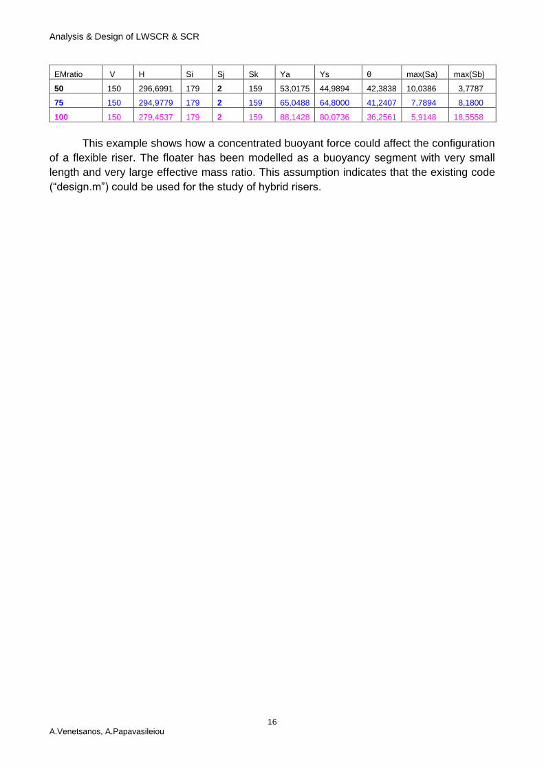
EMratio V H Si Sj Sk Ya Ys θ max(Sa) max(Sb)
50 150 296,6991 179 2 159 53,0175 44,9894 42,3838 10,0386 3,7787
75 150 294,9779 179 2 159 65,0488 64,8000 41,2407 7,7894 8,1800
100 150 279,4537 179 2 159 88,1428 80,0736 36,2561 5,9148 18,5558
This example shows how a concentrated buoyant force could affect the configuration
of a flexible riser. The floater has been modelled as a buoyancy segment with very small
length and very large effective mass ratio. This assumption indicates that the existing code
(“design.m”) could be used for the study of hybrid risers.
Analysis & Design of LWSCR & SCR
17 A.Venetsanos, A.Papavasileiou
Chapter 5 – Hang-off point offset
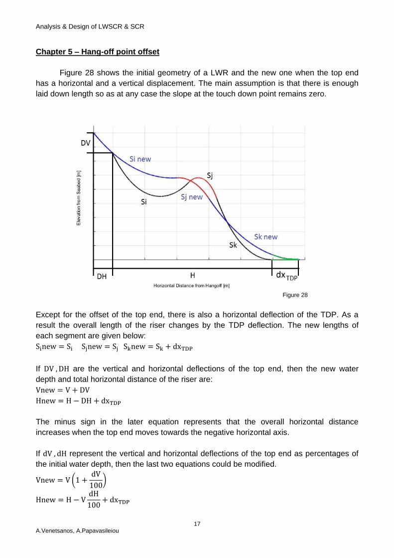
Figure 28 shows the initial geometry of a LWR and the new one when the top end
has a horizontal and a vertical displacement. The main assumption is that there is enough
laid down length so as at any case the slope at the touch down point remains zero.
Figure 28
Except for the offset of the top end, there is also a horizontal deflection of the TDP. As a
result the overall length of the riser changes by the TDP deflection. The new lengths of
each segment are given below:
Sinew = Si Sjnew = Sj Sknew = Sk + dxTDP
If DV , DH are the vertical and horizontal deflections of the top end, then the new water
depth and total horizontal distance of the riser are:
Vnew = V + DV
Hnew = H − DH + dxTDP
The minus sign in the later equation represents that the overall horizontal distance
increases when the top end moves towards the negative horizontal axis.
If dV , dH represent the vertical and horizontal deflections of the top end as percentages of
the initial water depth, then the last two equations could be modified.
Vnew = V (1 +dV
100)
Hnew = H − VdH
100+ dxTDP
Analysis & Design of LWSCR & SCR
18 A.Venetsanos, A.Papavasileiou
The above modifications are useful during preliminary design because the majority of
regulations express the allowed deflections of the floating platforms as percentages of the
water depth.
If dV , dH are known, then the new shape of the riser could be determined iteratively in the
same way as the initial one was determined when the hang-off, the buoyancy and the
touchdown catenary lengths were known [1]. The only difference is that there is one more
unknown variable and one more equation for the check of the convergence. To conclude,
the unknown variables are:
New hang-off angle: θnew
TDP deflection: dxTDP
The converge criteria are:
|y1 − y2 − y3 + y4 + y5 − Vnew
Vnew| ≤ ε
|x1 − x2 − x3 + x4 + x5 − Hnew
Hnew| ≤ ε
The allowed error of the results could be specified by the selection of the very small number
(ε). The matlab non linear solver “fsolve” which was used, specifies the above tolerance by
default.
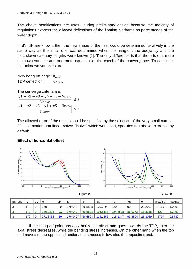
Effect of horizontal offset
Figure 29 Figure 30
EMratio V dV H dH Si Sj Sk Ya Ys θ max(Sa) max(Sb)
3 170 0 250 0 170,9427 60,5598 129,7893 120 90 22,2001 4,3165 1.0962
3 170 0 230,0295 10 170,9427 60,5598 126,8188 124,3598 86,9373 18,8288 4,127 1,3459
3 170 0 271,3463 -10 170,9427 60,5598 134,1356 115,1347 93,3504 26,3069 4,5797 0,8732
If the hang-off point has only horizontal offset and goes towards the TDP, then the axial stress decreases, while the bending stress increases. On the other hand when the top end moves to the opposite direction, the stresses follow also the opposite trend.
Analysis & Design of LWSCR & SCR
19 A.Venetsanos, A.Papavasileiou
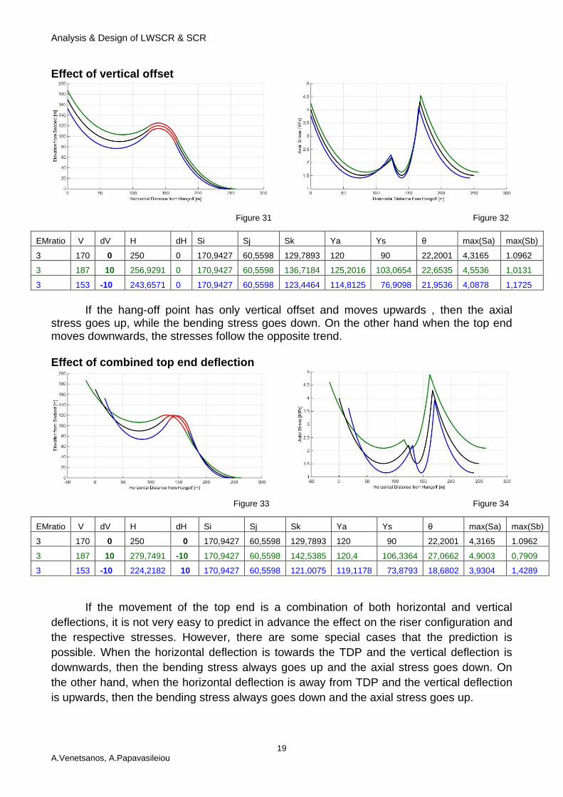
Effect of vertical offset
Figure 31 Figure 32
EMratio V dV H dH Si Sj Sk Ya Ys θ max(Sa) max(Sb)
3 170 0 250 0 170,9427 60,5598 129,7893 120 90 22,2001 4,3165 1.0962
3 187 10 256,9291 0 170,9427 60,5598 136,7184 125,2016 103,0654 22,6535 4,5536 1,0131
3 153 -10 243,6571 0 170,9427 60,5598 123,4464 114,8125 76,9098 21,9536 4,0878 1,1725
If the hang-off point has only vertical offset and moves upwards , then the axial
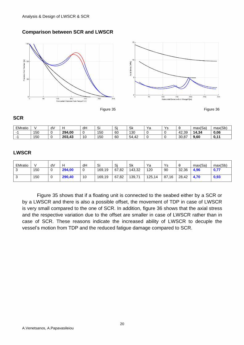
stress goes up, while the bending stress goes down. On the other hand when the top end moves downwards, the stresses follow the opposite trend. Effect of combined top end deflection
Figure 33 Figure 34
EMratio V dV H dH Si Sj Sk Ya Ys θ max(Sa) max(Sb)
3 170 0 250 0 170,9427 60,5598 129,7893 120 90 22,2001 4,3165 1.0962
3 187 10 279,7491 -10 170,9427 60,5598 142,5385 120,4 106,3364 27,0662 4,9003 0,7909
3 153 -10 224,2182 10 170,9427 60,5598 121,0075 119,1178 73,8793 18,6802 3,9304 1,4289
If the movement of the top end is a combination of both horizontal and vertical
deflections, it is not very easy to predict in advance the effect on the riser configuration and
the respective stresses. However, there are some special cases that the prediction is
possible. When the horizontal deflection is towards the TDP and the vertical deflection is
downwards, then the bending stress always goes up and the axial stress goes down. On
the other hand, when the horizontal deflection is away from TDP and the vertical deflection
is upwards, then the bending stress always goes down and the axial stress goes up.
Analysis & Design of LWSCR & SCR
20 A.Venetsanos, A.Papavasileiou
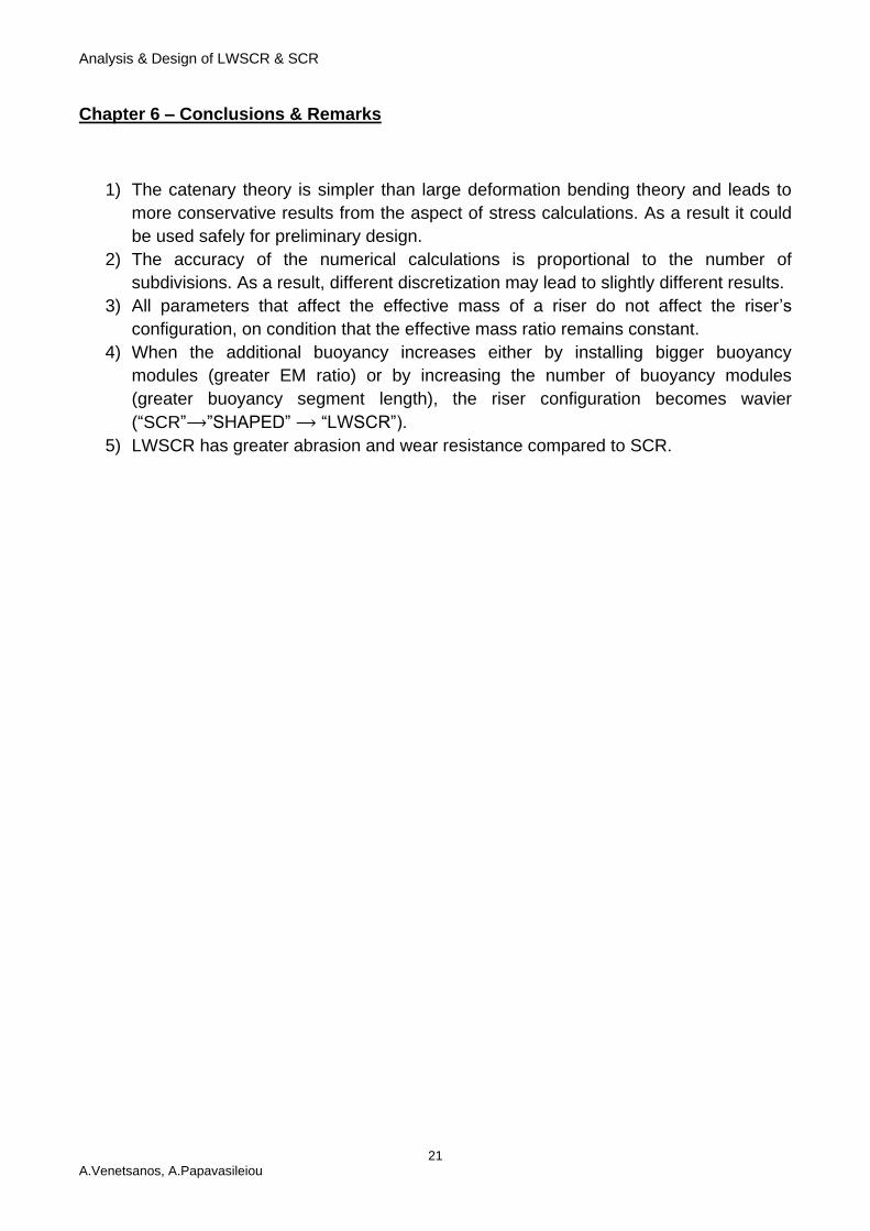
Comparison between SCR and LWSCR
Figure 35 Figure 36
SCR
EMratio V dV H dH Si Sj Sk Ya Ys θ max(Sa) max(Sb)
-1 150 0 294,00 0 150 60 130 0 0 42,39 14,34 0,06
-1 150 0 203,43 10 150 60 54,42 0 0 30,87 9,60 0,11
LWSCR
EMratio V dV H dH Si Sj Sk Ya Ys θ max(Sa) max(Sb)
3 150 0 294,00 0 169,19 67,82 143,32 120 90 32,36 4,96 0,77
3 150 0 290,40 10 169,19 67,82 139,71 125,14 87,16 28,42 4,70 0,93
Figure 35 shows that if a floating unit is connected to the seabed either by a SCR or
by a LWSCR and there is also a possible offset, the movement of TDP in case of LWSCR
is very small compared to the one of SCR. In addition, figure 36 shows that the axial stress
and the respective variation due to the offset are smaller in case of LWSCR rather than in
case of SCR. These reasons indicate the increased ability of LWSCR to decuple the
vessel’s motion from TDP and the reduced fatigue damage compared to SCR.
Analysis & Design of LWSCR & SCR
21 A.Venetsanos, A.Papavasileiou
Chapter 6 – Conclusions & Remarks
1) The catenary theory is simpler than large deformation bending theory and leads to
more conservative results from the aspect of stress calculations. As a result it could
be used safely for preliminary design.
2) The accuracy of the numerical calculations is proportional to the number of
subdivisions. As a result, different discretization may lead to slightly different results.
3) All parameters that affect the effective mass of a riser do not affect the riser’s
configuration, on condition that the effective mass ratio remains constant.
4) When the additional buoyancy increases either by installing bigger buoyancy
modules (greater EM ratio) or by increasing the number of buoyancy modules
(greater buoyancy segment length), the riser configuration becomes wavier
(“SCR”⟶”SHAPED” ⟶ “LWSCR”).
5) LWSCR has greater abrasion and wear resistance compared to SCR.
Analysis & Design of LWSCR & SCR
22 A.Venetsanos, A.Papavasileiou
References
1. S. Li, C. Nguyen, Dec 2010, Dynamic Response of Deepwater Lazy-Wave Catenary
Riser, DOT International.
2. C.P. Sparks, 2007, Fundamentals of Marine Riser Mechanics, PennWell Corporation
3. M. Grasselli, D. Pelinovsky, 2008, Numerical Mathematics, Jones and Barlett
Publishers
4. J.E. Dennis, Jr. R. B. Schnabel, Numerical Methods for Unconstrained Optimization
and Nonlinear Equations, SIAM
Analysis & Design of LWSCR & SCR
23 A.Venetsanos, A.Papavasileiou
Appendix
“design.m”
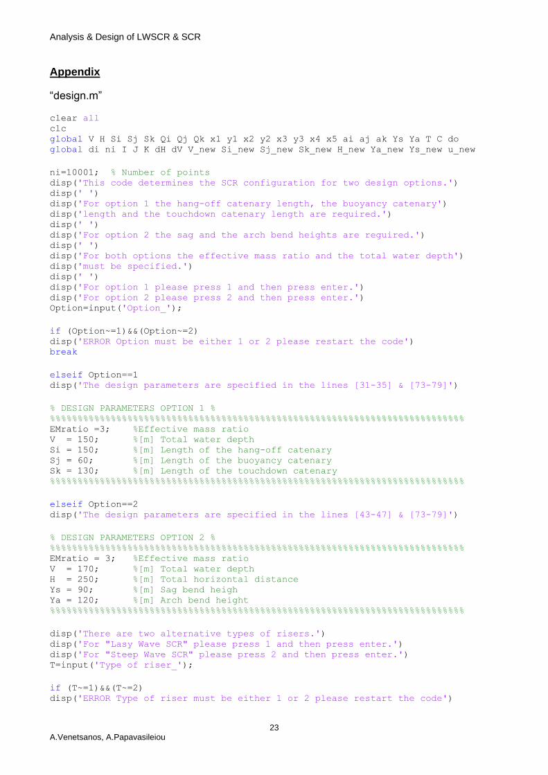
clear all clc global V H Si Sj Sk Qi Qj Qk x1 y1 x2 y2 x3 y3 x4 x5 ai aj ak Ys Ya T C do global di ni I J K dH dV V_new Si_new Sj_new Sk_new H_new Ya_new Ys_new u_new
ni=10001; % Number of points disp('This code determines the SCR configuration for two design options.') disp(' ') disp('For option 1 the hang-off catenary length, the buoyancy catenary') disp('length and the touchdown catenary length are required.') disp(' ') disp('For option 2 the sag and the arch bend heights are reguired.') disp(' ') disp('For both options the effective mass ratio and the total water depth') disp('must be specified.') disp(' ') disp('For option 1 please press 1 and then press enter.') disp('For option 2 please press 2 and then press enter.') Option=input('Option_');
if (Option~=1)&&(Option~=2) disp('ERROR Option must be either 1 or 2 please restart the code') break
elseif Option==1 disp('The design parameters are specified in the lines [31-35] & [73-79]')
% DESIGN PARAMETERS OPTION 1 % %%%%%%%%%%%%%%%%%%%%%%%%%%%%%%%%%%%%%%%%%%%%%%%%%%%%%%%%%%%%%%%%%%%%%%%%%%% EMratio =3; %Effective mass ratio V = 150; %[m] Total water depth Si = 150; %[m] Length of the hang-off catenary Sj = 60; %[m] Length of the buoyancy catenary Sk = 130; %[m] Length of the touchdown catenary %%%%%%%%%%%%%%%%%%%%%%%%%%%%%%%%%%%%%%%%%%%%%%%%%%%%%%%%%%%%%%%%%%%%%%%%%%%
elseif Option==2 disp('The design parameters are specified in the lines [43-47] & [73-79]')
% DESIGN PARAMETERS OPTION 2 % %%%%%%%%%%%%%%%%%%%%%%%%%%%%%%%%%%%%%%%%%%%%%%%%%%%%%%%%%%%%%%%%%%%%%%%%%%% EMratio = 3; %Effective mass ratio V = 170; %[m] Total water depth H = 250; %[m] Total horizontal distance Ys = 90; %[m] Sag bend heigh Ya = 120; %[m] Arch bend height %%%%%%%%%%%%%%%%%%%%%%%%%%%%%%%%%%%%%%%%%%%%%%%%%%%%%%%%%%%%%%%%%%%%%%%%%%%
disp('There are two alternative types of risers.') disp('For "Lasy Wave SCR" please press 1 and then press enter.') disp('For "Steep Wave SCR" please press 2 and then press enter.') T=input('Type of riser_');
if (T~=1)&&(T~=2) disp('ERROR Type of riser must be either 1 or 2 please restart the code')
Analysis & Design of LWSCR & SCR
24 A.Venetsanos, A.Papavasileiou
break end
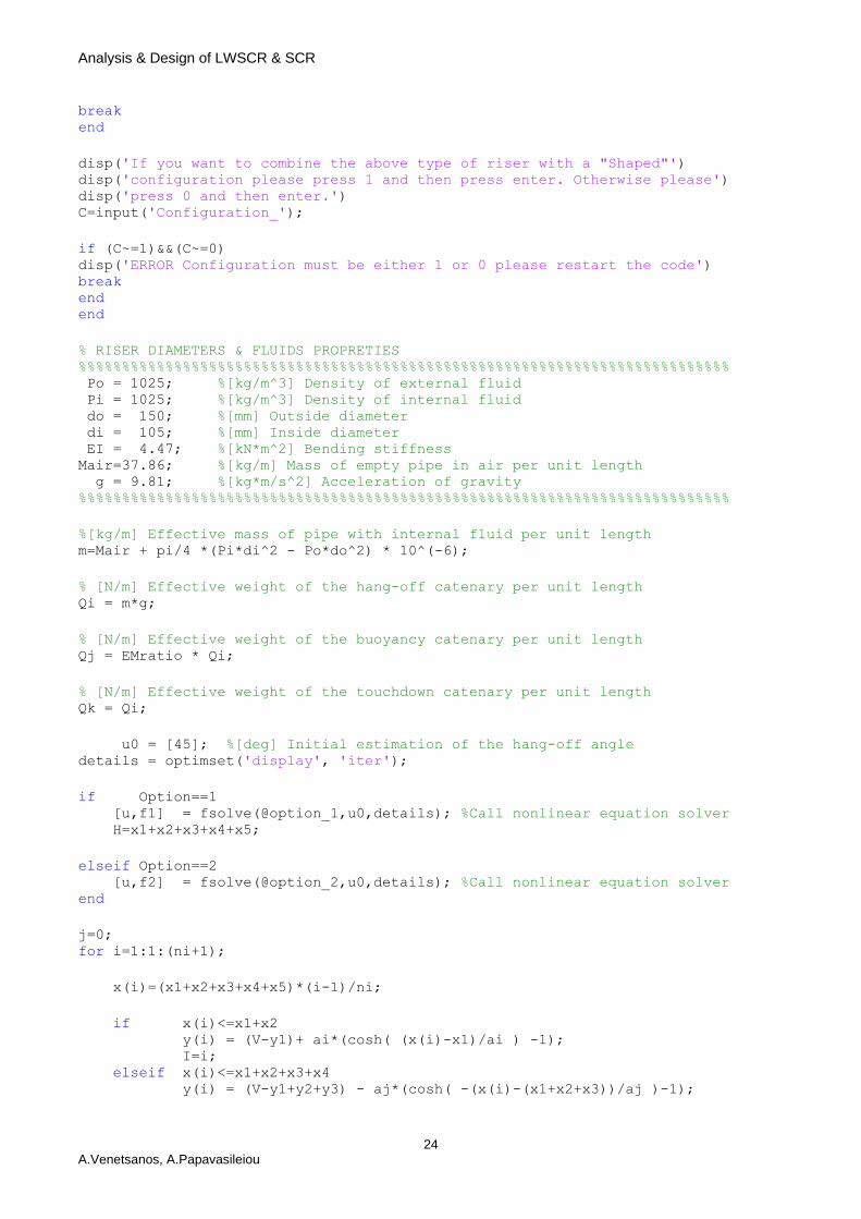
disp('If you want to combine the above type of riser with a "Shaped"') disp('configuration please press 1 and then press enter. Otherwise please') disp('press 0 and then enter.') C=input('Configuration_');
if (C~=1)&&(C~=0) disp('ERROR Configuration must be either 1 or 0 please restart the code') break end end
% RISER DIAMETERS & FLUIDS PROPRETIES %%%%%%%%%%%%%%%%%%%%%%%%%%%%%%%%%%%%%%%%%%%%%%%%%%%%%%%%%%%%%%%%%%%%%%%%%%% Po = 1025; %[kg/m^3] Density of external fluid Pi = 1025; %[kg/m^3] Density of internal fluid do = 150; %[mm] Outside diameter di = 105; %[mm] Inside diameter EI = 4.47; %[kN*m^2] Bending stiffness Mair=37.86; %[kg/m] Mass of empty pipe in air per unit length g = 9.81; %[kg*m/s^2] Acceleration of gravity %%%%%%%%%%%%%%%%%%%%%%%%%%%%%%%%%%%%%%%%%%%%%%%%%%%%%%%%%%%%%%%%%%%%%%%%%%%
%[kg/m] Effective mass of pipe with internal fluid per unit length m=Mair + pi/4 *(Pi*di^2 - Po*do^2) * 10^(-6);
% [N/m] Effective weight of the hang-off catenary per unit length Qi = m*g;
% [N/m] Effective weight of the buoyancy catenary per unit length Qj = EMratio * Qi;
% [N/m] Effective weight of the touchdown catenary per unit length Qk = Qi;
u0 = [45]; %[deg] Initial estimation of the hang-off angle details = optimset('display', 'iter');
if Option==1 [u,f1] = fsolve(@option_1,u0,details); %Call nonlinear equation solver H=x1+x2+x3+x4+x5;
elseif Option==2 [u,f2] = fsolve(@option_2,u0,details); %Call nonlinear equation solver end
j=0; for i=1:1:(ni+1);
x(i)=(x1+x2+x3+x4+x5)*(i-1)/ni;
if x(i)<=x1+x2 y(i) = (V-y1)+ ai*(cosh( (x(i)-x1)/ai ) -1); I=i; elseif x(i)<=x1+x2+x3+x4 y(i) = (V-y1+y2+y3) - aj*(cosh( -(x(i)-(x1+x2+x3))/aj )-1);
Analysis & Design of LWSCR & SCR
25 A.Venetsanos, A.Papavasileiou
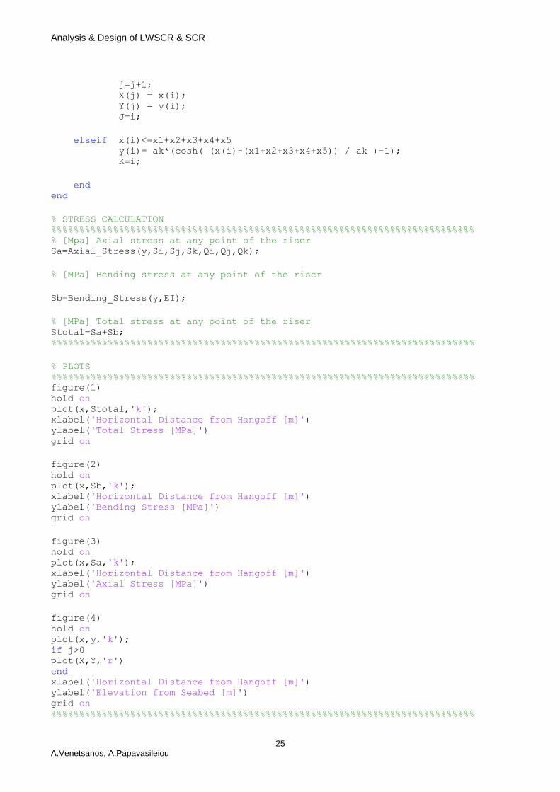
j=j+1; X(j) = x(i); Y(j) = y(i); J=i;
elseif x(i)<=x1+x2+x3+x4+x5 y(i)= ak*(cosh( (x(i)-(x1+x2+x3+x4+x5)) / ak )-1); K=i;
end end
% STRESS CALCULATION %%%%%%%%%%%%%%%%%%%%%%%%%%%%%%%%%%%%%%%%%%%%%%%%%%%%%%%%%%%%%%%%%%%%%%%%%%% % [Mpa] Axial stress at any point of the riser Sa=Axial_Stress(y,Si,Sj,Sk,Qi,Qj,Qk);
% [MPa] Bending stress at any point of the riser
Sb=Bending_Stress(y,EI);
% [MPa] Total stress at any point of the riser Stotal=Sa+Sb; %%%%%%%%%%%%%%%%%%%%%%%%%%%%%%%%%%%%%%%%%%%%%%%%%%%%%%%%%%%%%%%%%%%%%%%%%%%
% PLOTS %%%%%%%%%%%%%%%%%%%%%%%%%%%%%%%%%%%%%%%%%%%%%%%%%%%%%%%%%%%%%%%%%%%%%%%%%%% figure(1) hold on plot(x,Stotal,'k'); xlabel('Horizontal Distance from Hangoff [m]') ylabel('Total Stress [MPa]') grid on
figure(2) hold on plot(x,Sb,'k'); xlabel('Horizontal Distance from Hangoff [m]') ylabel('Bending Stress [MPa]') grid on
figure(3) hold on plot(x,Sa,'k'); xlabel('Horizontal Distance from Hangoff [m]') ylabel('Axial Stress [MPa]') grid on
figure(4) hold on plot(x,y,'k'); if j>0 plot(X,Y,'r') end xlabel('Horizontal Distance from Hangoff [m]') ylabel('Elevation from Seabed [m]') grid on %%%%%%%%%%%%%%%%%%%%%%%%%%%%%%%%%%%%%%%%%%%%%%%%%%%%%%%%%%%%%%%%%%%%%%%%%%%
Analysis & Design of LWSCR & SCR
26 A.Venetsanos, A.Papavasileiou
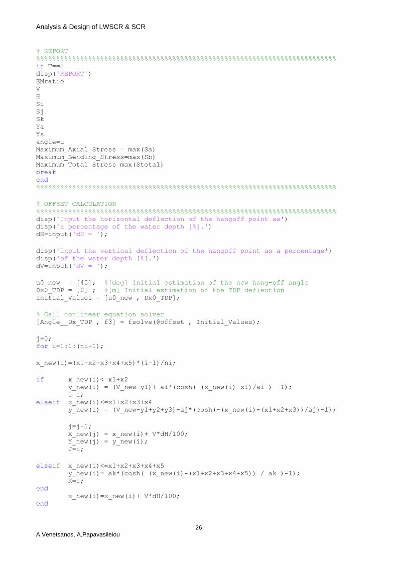
% REPORT %%%%%%%%%%%%%%%%%%%%%%%%%%%%%%%%%%%%%%%%%%%%%%%%%%%%%%%%%%%%%%%%%%%%%%%%%%% if T==2 disp('REPORT') EMratio V H Si Sj Sk Ya Ys angle=u Maximum_Axial_Stress = max(Sa) Maximum_Bending_Stress=max(Sb) Maximum_Total_Stress=max(Stotal) break end %%%%%%%%%%%%%%%%%%%%%%%%%%%%%%%%%%%%%%%%%%%%%%%%%%%%%%%%%%%%%%%%%%%%%%%%%%%
% OFFSET CALCULATION %%%%%%%%%%%%%%%%%%%%%%%%%%%%%%%%%%%%%%%%%%%%%%%%%%%%%%%%%%%%%%%%%%%%%%%%%%% disp('Input the horizontal deflection of the hangoff point as') disp('a percentage of the water depth [%].') dH=input('dH = ');
disp('Input the vertical deflection of the hangoff point as a percentage') disp('of the water depth [%].') dV=input('dV = ');
u0_new = [45]; %[deg] Initial estimation of the new hang-off angle Dx0_TDP = [0] ; %[m] Initial estimation of the TDP deflection Initial_Values = [u0_new , Dx0_TDP];
% Call nonlinear equation solver [Angle__Dx_TDP , f3] = fsolve(@offset , Initial_Values);
j=0; for i=1:1:(ni+1);
x_new(i)=(x1+x2+x3+x4+x5)*(i-1)/ni;
if x_new(i)<=x1+x2 y_new(i) = (V_new-y1)+ ai*(cosh( (x_new(i)-x1)/ai ) -1); I=i; elseif x_new(i)<=x1+x2+x3+x4 y_new(i) = (V_new-y1+y2+y3)-aj*(cosh(-(x_new(i)-(x1+x2+x3))/aj)-1);
j=j+1; X_new(j) = x_new(i)+ V*dH/100; Y_new(j) = y_new(i); J=i;
elseif x_new(i)<=x1+x2+x3+x4+x5 y_new(i)= ak*(cosh( (x_new(i)-(x1+x2+x3+x4+x5)) / ak )-1); K=i; end x_new(i)=x_new(i)+ V*dH/100; end
Analysis & Design of LWSCR & SCR
27 A.Venetsanos, A.Papavasileiou
%%%%%%%%%%%%%%%%%%%%%%%%%%%%%%%%%%%%%%%%%%%%%%%%%%%%%%%%%%%%%%%%%%%%%%%%%%%
% NEW STRESS CALCULATION %%%%%%%%%%%%%%%%%%%%%%%%%%%%%%%%%%%%%%%%%%%%%%%%%%%%%%%%%%%%%%%%%%%%%%%%%%% % [Mpa] New axial stress at any point of the riser Sa_new=Axial_Stress(y_new,Si_new,Sj_new,Sk_new,Qi,Qj,Qk);
% [MPa] New bending stress at any point of the riser
Sb_new=Bending_Stress(y_new,EI);
% [MPa] New total stress at any point of the riser Stotal_new=Sa_new+Sb_new; %%%%%%%%%%%%%%%%%%%%%%%%%%%%%%%%%%%%%%%%%%%%%%%%%%%%%%%%%%%%%%%%%%%%%%%%%%%
% PLOTS %%%%%%%%%%%%%%%%%%%%%%%%%%%%%%%%%%%%%%%%%%%%%%%%%%%%%%%%%%%%%%%%%%%%%%%%%%% figure(1) hold on plot(x_new,Stotal_new,'b'); xlabel('Horizontal Distance from Hangoff [m]') ylabel('Total Stress [MPa]') grid on
figure(2) hold on plot(x_new,Sb_new,'b'); xlabel('Horizontal Distance from Hangoff [m]') ylabel('Bending Stress [MPa]') grid on
figure(3) hold on plot(x_new,Sa_new,'b'); xlabel('Horizontal Distance from Hangoff [m]') ylabel('Axial Stress [MPa]') grid on
figure(4) hold on plot(x_new,y_new,'b'); if j>0 plot(X_new,Y_new,'r') end xlabel('Horizontal Distance from Hangoff [m]') ylabel('Elevation from Seabed [m]') grid on %%%%%%%%%%%%%%%%%%%%%%%%%%%%%%%%%%%%%%%%%%%%%%%%%%%%%%%%%%%%%%%%%%%%%%%%%%%
% REPORT %%%%%%%%%%%%%%%%%%%%%%%%%%%%%%%%%%%%%%%%%%%%%%%%%%%%%%%%%%%%%%%%%%%%%%%%%%% disp('REPORT') disp('Main design parameters when there is no deflection of the platform.') EMratio V H Si Sj Sk
Analysis & Design of LWSCR & SCR
28 A.Venetsanos, A.Papavasileiou
Ya Ys angle=u Maximum_Axial_Stress = max(Sa) Maximum_Bending_Stress=max(Sb) Maximum_Total_Stress=max(Stotal)
disp('Main design parameters when there is horizontal & vertical offset.') EMratio V_new dV H_new dH Si_new Sj_new Sk_new Ya_new Ys_new angle_new=u_new Maximum_Axial_Stress = max(Sa_new) Maximum_Bending_Stress=max(Sb_new) Maximum_Total_Stress=max(Stotal_new)
disp('If you want to see the authors of this code please press 1 and then') disp('press enter, else press any other number.') D=input('');
if D==1 load('Z','A') figure('units','normalized','outerposition',[0 0 1 1]) hold on image(A) end
Analysis & Design of LWSCR & SCR
29 A.Venetsanos, A.Papavasileiou
“option_1.m” function f1 = option_1(u)
global V Si Sj Sk Qi Qj x1 y1 x2 y2 x3 y3 x4 y4 x5 y5 ai aj ak Ys Ya
if Sk==0 disp('This part of the code does not support Steep Wave Riser design.') disp('Please sellect a positive Sk value and restart the code.') return end
v = u*pi/180; %[rad] hang-off angle
S = Si+Sj+Sk; ai = (S -(1+Qj/Qi) *Sj)*tan(v); aj = Qi/Qj *ai; ak = ai;
S1 = S-(1+Qj/Qi)*Sj;
x1 = ai * asinh(cot(v)); y1 = ai * (cosh(x1/ai)-1);
x2 = ai * asinh((Si-S1)/ai); y2 = ai * (cosh(x2/ai)-1);
x3 = x2*Qi/Qj; y3 = y2*Qi/Qj;
S4 = Qi/Qj *(S-Si-Sj); x4 = aj * asinh(S4/aj); y4 = aj * (cosh(x4/aj)-1);
x5 = ai * asinh((S-Si-Sj)/ai); y5 = y4*Qj/Qi;
Ys = y4+y5-y2-y3; Ya = y4+y5;
f1=y1+y4+y5-y2-y3-V;
Analysis & Design of LWSCR & SCR
30 A.Venetsanos, A.Papavasileiou
“option_2.m” function f2 = option_2(u)
global V H Si Sj Sk Qi Qj x1 y1 x2 y2 x3 y3 x4 y4 x5 y5 ai aj ak Ys Ya T C
v = u*pi/180; %[rad] hang-off angle y1=abs(V-Ys);
ai=y1/(cosh(asinh(cot(v)))-1); aj=ai*Qi/Qj; ak=ai;
x1=(ai*asinh(cot(v)));
y2=(Qj*(Ya-Ys)/(Qi+Qj)); y3=(Qi*(Ya-Ys)/(Qi+Qj));
if C==0 x2=(ai*acosh(y2/ai +1)); x3=(aj*acosh(y3/aj +1));
elseif C==1 x2=-(ai*acosh(y2/ai +1)); x3=-(aj*acosh(y3/aj +1)); end
if T==1 y4=(Qi*Ya/(Qi+Qj)); y5=(Qj*Ya/(Qi+Qj));
x4=aj*acosh(y4/aj +1); x5=ai*acosh(y5/ai +1);
elseif T==2 y4=Ya; y5=0;
x4=aj*acosh(y4/aj +1); x5=0; end
Si=ai*(sinh(x1/ai)+sinh(x2/ai)); Sj=aj*(sinh(x3/aj)+sinh(x4/aj)); Sk=ai*sinh(x5/ai);
f2=x1+x2+x3+x4+x5-H;
Analysis & Design of LWSCR & SCR
31 A.Venetsanos, A.Papavasileiou
“Axial_Stress.m” function Sa=Axial_Stress(y,Si,Sj,Sk,Qi,Qj,Qk)
global do di Dy ni x1 x2 x3 x4 x5
% Numerical approximation of the first differece h=(x1+x2+x3+x4+x5)/ni; for i=1:1:(ni+1) if i==1 || i==2 % Forward diff. aprox. Dy(i)=(-y(i+2) + 4*y(i+1) - 3*y(i)) / (2*h);
elseif i==ni || i==ni+1 % Backward diff. aprox. Dy(i)=(3*y(i) - 4*y(i-1) + y(i-2)) / (2*h);
else % Central diff. aprox. Dy(i)=(-y(i+2) + 8*y(i+1) - 8*y(i-1) + y(i-2)) / (12*h); end
Dy(i)=abs(Dy(i)); end
% Vertical component of top tension Ttop_y = Si*Qi-Sj*Qj+Sk*Qk;
% Horizontal component of top tension Ttop_x = ( Ttop_y / Dy(1) );
for i=1:1:ni+1 % [N] Axial force at any point of the riser T(i) = Ttop_x / (cos( atan( Dy(i)) ));
% [Mpa] Axial stress at any point of the riser Sa(i) = abs( T(i)/( (do^2 - di^2)*pi/4 )); end
Analysis & Design of LWSCR & SCR
32 A.Venetsanos, A.Papavasileiou
“Bending_Stress.m” function Sb=Bending_Stress(y,EI)
global x1 x2 x3 x4 x5 di do Dy ni I J K T
% Numerical approximation of the second difference
h=(x1+x2+x3+x4+x5)/ni; for i=1:1:(ni+1); if i<=I/2 % Forward diff. aprox. DDy(i)=(y(i+2) - 2*y(i+1) + y(i)) / h^2;
elseif i>I/2 && i<=I % Backward diff. aprox. DDy(i)=(y(i)-2*y(i-1)+y(i-2))/h^2;
elseif i>=I && i<=(I+J)/2 % Forward diff. aprox. DDy(i)=(y(i+2) - 2*y(i+1) + y(i)) / h^2;
elseif i>(I+J)/2 && i<=J % Backward diff. aprox. DDy(i)=(y(i)-2*y(i-1)+y(i-2))/h^2;
elseif i>=J && i<=(J+K)/2 % Forward diff. aprox. DDy(i)=(y(i+2) - 2*y(i+1) + y(i)) / h^2;
elseif i>(J+K)/2 && i<=K % Backward diff. aprox. DDy(i)=(y(i)-2*y(i-1)+y(i-2))/h^2; end end
for i=1:1:ni+1 KK(i)= abs(DDy(i) / (1+(Dy(i))^2)^(3/2) ); %[m^(-1)] Curvature end
% Curvature approximation at the points of discontinuity
if J~=[] KK(I) = 0.5*KK(I-1) + 0.5*KK(I+1); end if K~=[] KK(J) = 0.5*KK(J-1) + 0.5*KK(J+1); end
ro=do/2000; %[m] Outside radius ri=di/2000; %[m] Inside radius Ia=(ro^4 - ri^4)*pi/4; %[m^4] Second moment of area Sb=(KK*EI*ro/Ia)*10^(-3); %[MPa] Bending stress
Analysis & Design of LWSCR & SCR
33 A.Venetsanos, A.Papavasileiou
“offset.m” function f3 = offset(Angle__Dx_TDP)
global V H Si Sj Sk Qi Qj x1 y1 x2 y2 x3 y3 x4 x5 ai aj ak global dH dV V_new Si_new Sj_new Sk_new H_new Ya_new Ys_new u_new
u_new = Angle__Dx_TDP(1); Dx_TDP = Angle__Dx_TDP(2);
Si_new=Si; Sj_new=Sj; Sk_new=Sk+Dx_TDP;
H_new=H - V*dH/100+Dx_TDP; V_new=V*(1+dV/100);
v = u_new * pi/180;
S = Si_new + Sj_new + Sk_new; ai = (S -(1+Qj/Qi) *Sj_new)*tan(v); aj = Qi/Qj *ai; ak = ai;
S1 = S-(1+Qj/Qi)*Sj_new;
x1 = ai * asinh(cot(v)); y1 = ai * (cosh(x1/ai)-1);
x2 = ai * asinh((Si_new-S1)/ai); y2 = ai * (cosh(x2/ai)-1);
x3 = x2*Qi/Qj; y3 = y2*Qi/Qj;
S4 = Qi/Qj *(S-Si_new-Sj_new); x4 = aj * asinh(S4/aj); y4 = aj * (cosh(x4/aj)-1);
x5 = ai * asinh((S-Si_new-Sj_new)/ai); y5 = y4*Qj/Qi;
Ys_new = y4+y5-y2-y3; Ya_new = y4+y5;
f3 = [y1+y4+y5-y2-y3-V_new ; x1+x2+x3+x4+x5-H_new];