Moral Hazard and Collateral as Screening Device:

Empirical and Experimental Evidence+

C. Mónica Capra*

Matilde O. Fernandez†

and

Irene Ramirez-Comeig‡

+ Information provided by the Sociedad de Garantia Reciproca de la Comunidad Valenciana (Reciprocal Guarantee Company of Land of Valencia) is gratefully acknowledged. The authors thank anonymous referees for valuable comments and suggestions. * Department of Economics, Emory University, Atlanta, GA 30322, mcapra@emory.edu † Departamento de Finanzas Empresariales, Facultad de Economía, Universidad de Valencia, Valencia (Spain); E-mail: Matilde.Fernandez@uv.es ‡ Corresponding autor. Departamento de Finanzas Empresariales and LINEEX, Facultad de Economía, Universidad de Valencia, Valencia (Spain); E-mail:Irene.Ramirez@uv.es.

Moral Hazard and Collateral as Screening Device: Empirical and

Experimental Evidence

Abstract

This paper tests the separating role of contracts that involve both interest rates and

collateral in credit markets with asymmetric information. To test this prediction data

from real credit markets and controlled experiments are used. Using a sample of credits

to small and medium-sized firms in Valencia, Spain, we relate two different types of

contracts with an objective approximation to each ex ante borrower risk, i. e., the real

outcome of each loan and other relevant variables. Moreover, two incentive compatible

contracts are designed and decisions analyzed under two different experimental

treatments, one with moral hazard. Results confirm that borrowers of lower risk choose

contracts with higher collateral and a lower interest rate. However, it is ascertained that

moral hazard reduces separation.

JEL classification: G21, D82, C92

Keywords: Asymmetric Information, Collateral, Credit Markets, Experiments, Incentive

Compatible Contracts, Moral Hazard.

1. Introduction

Leading theoretical studies about the role of collateral in credit markets with

asymmetric information1 consider the effect of collateral in an isolated manner showing

that adverse selection and moral hazard imply that riskier credit applicants select high

collateral requirements (Stiglitz and Weiss, 1981 and Wette, 1983). Later analyses by

Bester (1985b) and Chan and Kanatas (1985) demonstrate that, by treating collateral

requirements together with variations in interest rates, collateral is negatively related to

1 The type of collateral on which the greatest part of theoretical work concerning asymmetric information is based, is external collateral, i.e., collateral in form of assets which do not belong to the company; assets which the lender might otherwise not claim. Only a very small number of papers deals with the role of internal collateral, i.e., collateral in form of assets of the business itself (see Smith and Warner (1979), Stulz and Johnson (1985) and Gorton and Kahn (2000)). Here we concentrate merely on the first type.

1

the borrower’s risk.2 Bester (1985b) shows that lenders are capable of indirectly

distinguishing between borrowers of different risk levels by offering pairs of incentive

compatible contracts with different interest rate-collateral combinations. In his later

work, Bester (1987) considers moral hazard because of ex ante asymmetric information

and reinforces previous conclusions. In addition, he suggests that the demanded

collateral softens the effects of moral hazard, since higher collateral gives incentives to

borrowers to choose projects involving a smaller risk.3 The possibility of separating

borrowers by their risk level is of great importance because of its consequences on

credit rationing and, hence, on the effectiveness of monetary policies by central banks.4

When creditors offer a menu of contracts inducing the selection of firms, there is a

separating equilibrium that reveals information and can resolve rationing. 5

Notwithstanding the relevance of these results, the hypothesis that contracts

combining pairs of collateral and interest rates are incentive compatible for borrowers

with different risk levels is yet to be verified empirically. Unfortunately, empirical tests

of the theories of the static relationship between collateral and credit risk are difficult to

conduct because of the scarcity of micro data on the contractual terms of commercial

bank loans, which are usually confidential. In spite of this, some evidence has been

generated on the effect of collateral in an isolated manner. Hester (1979), Leeth and

Scott (1989), Berger and Udell (1990), Boot, Thakor and Udell (1991) and Machauer

and Weber (1998) examine the characteristics of loans with collateral to establish a

2 See, also, Stiglitz and Weiss (1986, 1992), Besanko and Thakor (1987), Bester (1987), Deshons and Freixas (1987), Igawa and Kanatas (1990), Boot, Thakor and Udell (1991) and Coco (1999). 3 A more detailed discussion of the existing theoretical literature can be found in Coco (2000) 4 To classify borrowers, other studies introduce loans of variable sizes (Bester (1985a), Milde and Riley (1988) and Grinblatt and Hwang (1989)). On the other hand, work by Leland and Pyle (1977) and Brennan and Kraus (1987) suggests that the firm’s equity could be used to classify borrowers. 5 Not all studies that consider collateral as a mechanism to learn about the risk level of borrowers reach these conclusions. Work by Leland and Pyle (1977) and Stiglitz and Weiss (1986, 1992) also use collateral requirements and show that these might not be enough to eliminate credit rationing.

2

relationship between collateral and risk6. All these papers, except Machauer and

Weber, show that collateral is greatly correlated to higher risk. Most of this research

uses measures of ex ante observable risk to approximate to the real borrower risk of a

concrete loan. Hester (1979) and Machauer and Weber (1998) concentrate on the

borrower credit rating. Leeth and Scott (1989) use the “company age”. Berger and

Udell (1990), who developed two tests, use the risk premium of the interest rate in the

first one. The loan risk premium (dependent variable) is regressed on measures of

collateral and on several control variables in a cross-section analysis. In the second test,

introducing a novelty in this kind of research, they try to corroborate their previous

results by examining the performance of borrowers and loans on an ex post basis. Net

charge-offs (charge-offs minus recoveries) as a measure of loan risk and several non-

performing characteristics (past due, nonaccrual and renegotiated status) are used as

measures of borrower risk. However, as the required data is not individually reported,

aggregate data are used. Our analysis differs from previous empirical work because our

database allows us to use a more direct approximation to each credit applicant risk level

(privately known to him/her and, consequently, ex ante unobservable), i.e. his/her real

or ex post insolvency.

Also, this paper differs from previous work as we analyze the effect of the

combination collateral/interest rate in each loan under moral hazard, which allows us to

test the empirical implications of theoretical models concerning the role of collateral in

incentive compatible contracts. Moreover, as far as we know, we present the first

experimental study in this field. According to most of the previous papers, and also

limited by our database, our analysis is restricted to small and medium-sized firms.

6 Moreover, Orgler (1970) evaluates credit applications including collateral as an explanatory variable so that, indirectly, evidence is provided on the relationship between collateral and credit risk.

3

We first use data collected from real credit markets considering two types of

contracts: one with external collateral and a low interest rate, and the other without

collateral and a high interest rate. The hypothesis to be tested is that by offering this

menu of contracts credit applicants are “separated” according to their ex ante

unobservable risk. Given the limitations we face with the data, we propose to

complement our study with experiments. In particular, we design an experiment that

would control for some key factors, such as moral hazard.

In the next section, the theoretical model and contrast hypotheses are presented.

In section 3, the empirical analysis, the database, the design of the test and its results are

described. In section 4, the experimental design, the treatments, and the results from the

experiment are presented. The final section summarizes the main conclusions and

results.

2. Theoretical model and contrast hypothesis

Our analysis follows Bester’s (1985 and 1987) models. Bester (1985) considers

a credit market with Ni risk neutral firms, which can either be type i = a or b, according

to the level of risk of their projects. Each firm has the possibility of starting a project

that requires an initial fixed investment I.7 The return on the project for firm i is given

by the random variable ~R i, with 0< ~R i < ⎯R i and a distribution function Fi(R) > 0 for

all R > 08. As in Stiglitz and Weiss (1981), ~R b has a greater risk than ~R a according to

the second order stochastic dominance criterion9. The firms have an initial wealth W<I,

which together with a loan B = I-W finance the project. Given the size of the loan, B, a

credit contract γ = (r, C) is specified by the interest rate r and the collateral C.

Entrepreneurs may face collateralization costs assumed to be proportional the amount of

7 Given that the required investment is fixed, it is not used as a way to signal information about the risk of the loan applicant. See Milde and Riley (1988) for models in which the investment is used as a signal. 8 This condition ensures that there is a positive probability of failure as long as the interest payments exceed the collateral.

4

collateral. When C > (1+r)B, the firm would not admit project failure. Therefore, only

contracts with C < (1+r)B are considered. It is assumed that firm i’s project fails if C +

Ri < (1+r) B and this becomes observable only after a firm declares project failure. If

this happens, the bank becomes the owner of the investment project and its return.

Thus, the expected profit of the project for firm i and a credit contract γ is given by:

∏i(γ) = E{máx [ ~R i - (1+r) B - kC, -(1+k) C]} [1]

Banks cannot distinguish loan solicitors by risk; however, they can separate

them by offering a pair of contracts (γα, γβ) that are incentive compatible and act as self-

selecting mechanisms. The pair (γα, γβ) is incentive compatible if:

∏a(γα) > ∏a(γβ); ∏b(γβ) > ∏b(γα) [2]

Firm i will invest only if it receives a loan γ such that ∏i(γ) > (1+ π) W. As long

as a pair of contracts (γα, γβ) is offered, the firm prefers a contract that maximizes its

expected profits. Thus, if preferences of investors depend systematically on their types,

banks can utilize a menu of contracts with different collateral requirements as self-

selection mechanisms. In order to solve the problem of adverse selection, Bester (1985)

concludes that the low risk loan applicants try to differentiate themselves from high risk

applicants by accepting higher collateral as collateral is costly.

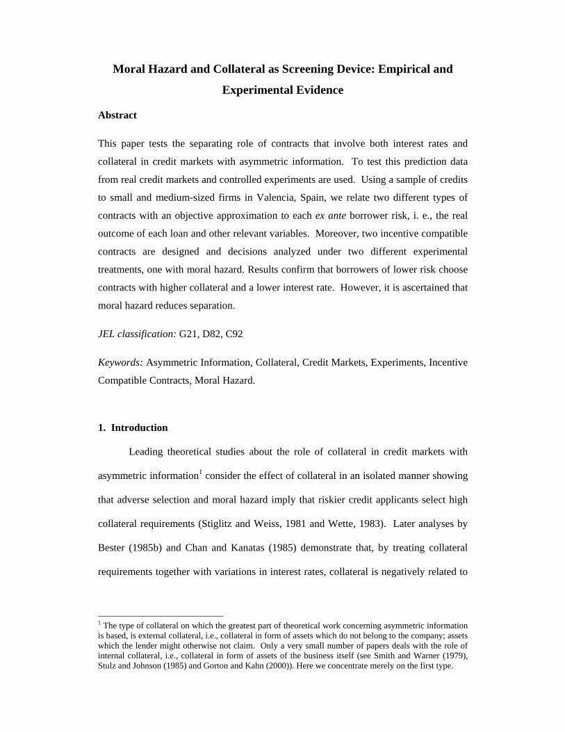
The isoprofit curves for the two types of loan applicants are depicted in Figure 1.

Applicant b’s isoprofit curve has a steeper slope than applicant a’s, because the first’s

project is riskier and, by stochastic dominance of second degree, profits are a convex

function of the realized returns (R). This means that type a firms are inclined to accept a

higher increment in collateral for a given reduction in interest rates than type b firms.

9 According to Rostchild and Stiglitz (1970)

5

This fact makes it possible for the bank to offer different pairs of incentive-compatible

contracts.10

Figure 1: Borrowers' isoprofit curves Source: Own elaboration

C

r

Cb Ca

ra

b

In addition to adverse selection, credit contracts also face incentive effects.

Perverse incentives arise when the firm has the possibility of choosing projects with

different risk levels. Bester (1987) studies this possibility. Moral hazard results from

the inability of lenders to control borrowers’ choices once the loan has been granted. It

is assumed that borrowers do not stop loan payments as long as the returns on the

investment allow repayment.11 The investment decision of the firm affects the failure

probability and, therefore, the profit of the lending firms. A few changes in the model

presented previously allow us to study these effects. Bester (1987) considers n

investment projects. Each project, i, with i = 1,...,n requires a fixed amount of

investment which is financed by a bank loan B. Project i provides a positive return on

investment Ri in case the project is successful, which happens with probability pi. The

10 In Bester (1985), self-selection resulted from stronger assumptions than in Stiglitz and Weiss (1981). To produce a separating equilibrium the additional assumption that Fi(R) > 0 for all R > 0 is needed. With this assumption, it is possible to have a monotonous relationship between risk and applicants’ preferences. 11 This hypothesis excludes another type of moral hazard present in Allen (1983) and Jaffee and Russell (1976). These authors assume that a borrower has an incentive to be opportunistic whenever the size of the loan is superior to the value of the collateral. In this paper, Bester assumes that the legal constraints exclude this possibility. In fact, the wealth of the borrowers is assumed to be lower than the loan. Collateral, then, can merely work as a signaling mechanism and an incentive mechanism. See Benjamin (1978) for an alternative role of collateral requirements.

6

project fails and provides no (0) return on investment with probability (1- pi). It is

assumed that 1> p1> p2>... > pn> 0 and B< R1< R2<... < Rn.12. There are N identical

firms in the market with the same initial endowment 0< W< B. Preferences over final

wealth are described by a von Neumann-Morgenstern utility function, U, where U´>0,

U´´<0. The expected utility of a firm that applies for a loan γ = (r, C, λ) is given by Vi

(γ) if project i is chosen, the parameter λ, 0< λ <1, is the probability of receiving the

loan. The banks then offer contracts γi under the condition that the applicant invests in

project i. However, since there is asymmetric information ex ante, these conditions

have to be self-imposed by the borrower. That is, credit contracts must be designed so

that project i is chosen when the borrower receives a loan γi (i.e., with loan γi she/he

should not want to choose a different project). Contract γi is incentive-compatible if:

Vi (γi) > Vj (γi) for all j [3]

Bester designs a loan contract as a problem of incentives because the interest

payments and collateral requirements affect the choice of the borrower. Thus, if the

contracts γi and γj are incentive-compatible and ri > rj, Ci < Cj and (ri, Ci) ≠ (rj, Cj),

Bester shows that project i will be riskier than project j (pi < pj). Indeed, if pj were less

than pi, the assumption of concavity of the utility function would be violated since Rj

>Ri. Bester concludes that an increase in the interest rate results in a negative effect

over the repayment probabilities, whereas an increase in collateral requirements results

in a positive effect. That is, an increase in collateral makes the riskier project less

attractive.

Our objective is to contrast and compare the Bester’s (1985) results about the

separating power of incentive compatible contracts defined as a collateral-rate pair and

12 As a special case of this assumption, projects can be differentiated by the second order stochastic dominance criterion as in Rostchild and Stiglitz (1970). The case, where piRi= pjRj, has been treated by Stiglitz and Weiss (1981), and Bester (1985).

7

the incentives that collateral requirements create when there is moral hazard (Bester

1987). Hence, in section 3, we measure the separating role using data from a sample of

credits given to small and medium size firms in Spain between 1982 and 1989. More

specifically, we test the following hypothesis: H1: two contracts, one with high

collateral and a low rate and the other without collateral and a higher rate allows

credit applicants to separate according to their risk levels. The lower risk borrower

chooses the first contract and the higher risk borrower chooses the second contract.

Experimental techniques can be used to overcome inherent obstacles in the data

collection of real markets by creating data under controlled environments; thus, in

section 4, we use experimental methods to analyze incentive compatibility in loan

contracts that combine collateral and interest rate requirements under two different

environments: first without moral hazard, and then with moral hazard due to ex ante

asymmetric information. The aim is to test the effect of moral hazard following Bester

(1987). Given that theoretically ad hoc incentive compatible contracts were designed,

we reformulate the hypotheses as described below to design two adequate tests.

Hypothesis H1E: By offering two incentive compatible contracts, borrowers can be

separated by their risk levels. Lower risk borrowers choose contracts with higher

collateral (Separating effect of collateral).

Hypothesis H2E: When there is moral hazard generated by ex ante asymmetric

information, higher collateral incentive borrowers choose lower risk projects (i.e., there

is a positive incentive effect of collateral).

3. Empirical Analysis

3.1 Cross-section data and test description

In the test we established a relationship between the dummy variable that

represents the combination collateral/interest rate for each individual borrower and an

8

objective approximation to the credit applicant ex ante risk level, i. e., his/her real or ex

post insolvency, and some control variables through an analysis of variance with one

factor (ANOVA) and through the logit analysis.

Our source of information is the Sociedad de Garantia Reciproca (SGR) of Land

of Valencia. The SGRs are financial entities that facilitate the access to credit to small

and medium-sized firms by guaranteeing loans these firms obtain from the banking

system.13 When SGRs guarantee a loan, there is a transfer of the credit risk from the

lender to the SGR. This means that, although SGRs do not give the loans, they accept

the risk of the loans. Hence, SGRs bear with the effects of asymmetric information and,

to mitigate its negative effects, they can decide to increase the collateral required or

ration credit.14

Only all SGR operations dealing with loans given to small and medium-sized

firms, i.e. firms with less than 250 employees,15 were considered16. Thus,

individualised information of 3,875 loans formalised from January 1st, 1982 to May 31st,

1998 is obtained. Of these, 2,729 (70%) had security provided by a guarantor, 305 (8%)

had real asset external collateral (i.e. assets not belonging to the company), and 841

(22%) had no collateral17. All loans correspond to PLCs, limited liability companies,

13 SGR are financial institutions that represent small and medium size firms and channel funds from banks that provide the loans. Their functions are to provide advise, assist and back firms. They are a hybrid between an anonymus society and cooperatives. They are for profit, but work under legal restrictions on how they divide the dividends (dividends must be accumulated as reserves in a guarantee fund). The SGR also receive help from the government. One of their tasks is to evaluate the risk of their clients’ projects before backing them. Althugh the SGR do not provide financing to firms, the gacilitate loans for small and medium size firms. Hence, the information that the SGR of Valencia provides about risk is useful since they are independent from the banks. To obtain further information on this type of societies in Spain and other countries, please refer to Ramirez-Comeig and Ferrando-Bolado (1999). 14 More precisely, the SGR can react rationing their guarantee, which can indirectly result in credit rationing, i. e if a small business does not have a SGR guarantee, it will find itself with more difficulties to access credit from the banking system. 15 The Law concerning SGRs states that a small and medium-sized firm is one that has less than two hundred and fifty employees. 16 The SGR of Valencia has provided us with an anonymous list of the individual characteristics of each of the transactions it backed since January 1982 until May 1998. A total of 24,355 transactions were recorded, 6,473 of which were loans given to firms with less than 250 workers. 17 In these contracts, the SRG does not require collateral, although all loans are backed by the SGR.

9

and sole proprietors. As the aim is to explore whether the borrowers with loans

combining high collateral with a low interest rate are less willing to take risks than those

with loans with a high interest rate and no collateral, only these two “extreme” groups

of loans were selected.18 Thus, loans are classified according to the difference between

the initial interest rate and the legal interest rate in Spain at the same time and term

(differential rate). Then, loans with a negative differential rate and real external

collateral and loans with a positive differential rate (2 percentage points) and no

collateral are chosen.

In this manner, we obtain individualized information concerning 323 loans

granted by 28 different financial institutions Among these loans, there are 172

combining real asset collateral with a low rate of interest, called Contract C2, and 151

loans combining no collateral with a higher interest rate, called Contract C1. We

expected the insolvency rate of the borrowers with Contract C2 to be significantly lower

than the one for borrowers with Contract C1. The variables used in this test are the

following:

- Endogenous variable:

CONTRACT: Dummy variable that summarizes the information about collateral and

interest rates of a loan being given a value of 0 for Contract C2 and 1 for Contract C1.

- Exogenous variables:

OUTC: Dummy variable that indicates the outcome of the loan being given a value of 0

if the outcome is insolvency and 1 otherwise. We define insolvency as the incapacity to

fulfil loan obligations, including temporary failure.

SIZE: Measures loan size in local currency, pesetas.

TERM: Defines the term of the loan in months.

18 Loans with an intermediate rate of interest and those with security provided by a guarantor were excluded as the objective was to deal with theoretically incentive-compatible contracts.

10

DEST: Dummy variable measuring the loan destination being given a value of 0 when

the loan is used to start a new business and 1 otherwise.

EMPL: Number of borrower’s employees.

FIRMTYPE: We used this variable in the analysis of variance to characterize the type of

the borrower’s firm being given a value of 0 for sole proprietors, 1 for limited

companies, and 2 for PLCs.19

FIRMTYPE (1): Given a value of 1 for sole proprietors and 0 for limited companies and

for PLCs.

FIRMTYPE (2): Given a value of 1 for limited companies and 0 for sole proprietors and

for PLCs.

The most relevant exogenous variable is the outcome of the loan, OUTC, since it

constitutes the approximation to the ex ante, i.e. privately known, borrower risk which

is the basis of the separating hypothesis. Given that this risk is not observable, an

approximation becomes necessary. Instead of using an indirect approximation, we use

the real or ex post loan outcome (0= insolvency, 1= otherwise) as it represents an

objective measure of the borrower risk concerning this particular loan. Our definition of

ex post insolvency includes any delaying payment, not only legal insolvency.20 The rest

of the variables play a double role. On the one hand, they specify information about the

type of loan or borrower related to each combination collateral/interest rate and, on the

other hand, they are also used as control variables since they are indicators of the ex

ante borrower’s risk. Unfortunately, our data base is not sufficient to consider all the

relevant control variables, which was taken into account at the time of the analysis of

19 In the logit analysis, we characterise the type of firm by the dummy variables FIRMTYPE(1) and FIRMTYPE(2). When both of these are given a value of 0, the firm is a PLC. 20 The real or ex post outcome of each loan is usually confidential information known only to the bank and the respective client. Therefore previous empirical research uses more or less indirect measures of the ex ante non-observable borrower risk. We had access to the ex post loan outcome from an anonymous database. Such database contained the most relevant characteristics of loans guaranteed by the SGR of Valencia from 1982 to 1998 , which we used as a proxy.

11

results. Using qualitative variables to measure collateral and interst rates we hope to

soften some of the seasonal and business cycle effects.21

Finally, to test whether the logit function is robust against a change in the

sample, the total sample is divided into two sub-samples. The estimation sub-sample is

composed of formalized loans from January 1st, 1983 to May 31st, 1998 consisting of

172 loans of Contract C2, and 131 loans of Contract C1. The validation sub-sample is

composed of the 20 loans formalized in 1982, all without collateral and high interest

rate.22

3.2.Empirical Results

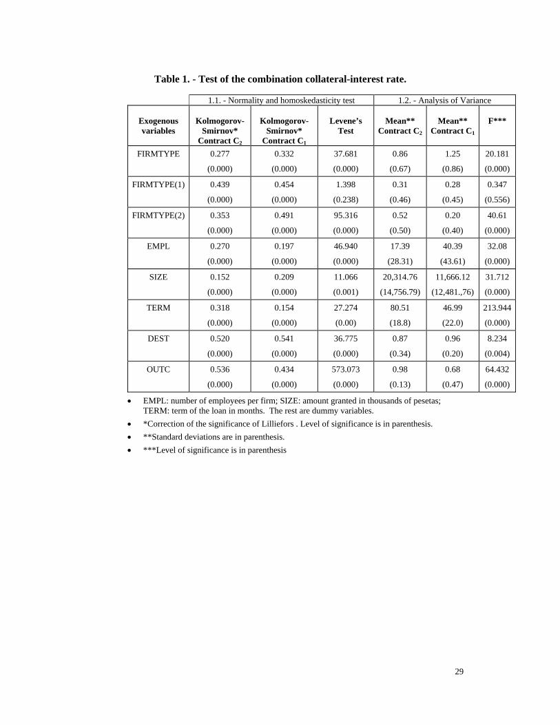
3.2.1 Results of the Analysis of Variance

Table 1 gives the results of the analysis of variance23. Each of the exogenous

variables clearly differentiate the two types of contracts, except FIRMTYPE(1); as

shown by the F statistics. Most of the firms with loans that combine real asset collateral

and low interest are limited companies and sole proprietors. PLCs have a greater

presence in the group of loans without collateral and with higher rates, as shown by the

mean values of the variables FIRMTYPE, FIRMTYPE (1) and FIRMTYPE (2).

Moreover, Contract C2 is held by companies with a smaller number of employees,

higher mean term and higher import than those opting for Contract C1. With respect to

the operation's destination, the weight of the loan for the establishment of new

businesses is higher in Contract C2, representing 13% of the total loans in this group,

while they represent only 4% of Contract C1 loans. Finally, OUTC variable shows that

21 We thank an anonimous referee to point us to this sigue. 22 The choice of the estimation subsample was made in order to have a homogenous and sufficient number of each type of contracts. However, we ran logit analysis using other selection criteria for subsamples and we obtained similar results. 23 Implicit hypotheses of the analysis of variance with one factor were tested, as shown in Table 1. Only FIRMTYPE(1) presents equal variance in the two types of loans. However, the lack of homogeneity of variance affects the F statistics if the ratio of the larger sample size to the smaller one is above 2, and in this case it is 1.13 (see, for instance, Uriel, 1995 and Cabrer et al., 2001). FIRMTYPE, FIRMTYPE(1),

12

the proportion of Contract C2 loans with insolvency problems is only 2%, whereas loans

without collateral and high rate present a much higher index of insolvency, 32%.

[INSERT TABLE 1]

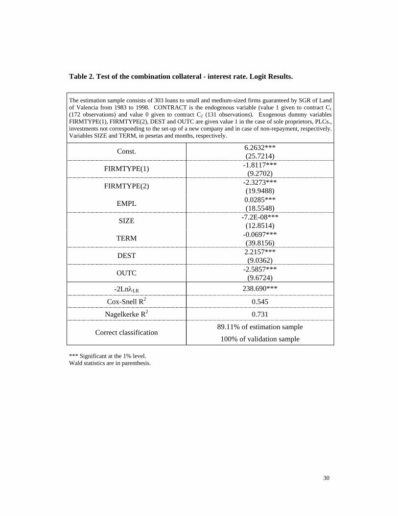
3.2.2 Results of the Logit Analysis

The variable selection method is the forward stepwise process of the likelihood

ratio. In Table 2 the results of the logit estimation and the variable selection are shown.

It is more likely that a loan formalizes with real asset collateral and low interests, the

higher the loan term, the larger the import, and the lower the number of employees in

the firm, in particular, if it is a sole proprietor or a company (PLC) and if funds obtained

by the loan are destined to the establishment of a new business. The results analyzed so

far reinforce the conclusion reached in the analysis of variance. When the loan presents

characteristics that make lenders presuppose a higher insolvency risk, they demand real

asset collateral. However, this higher ex ante risk is not translated into higher interest

rate requirements. The effect of the collateral has a greater weight than the interest rate

effect.

[INSERT TABLE 2]

OUTC coefficient implies that the loans with real asset collateral and low rate of

interest have no solvency problems, as observed in the ANOVA, despite the strong

collateral requirements were originated from higher borrower risk detected a priory by

the lender. In contrast, the loans without collateral and high interest rates have a high

probability of default.

With respect to the goodness of fit, Table 2 shows that each of the coefficients βj

is significantly different from zero. Globally, the model is also significant when

determining the probability of providing collateral combined with a low rate of interest.

FIRMTYPE(2), DEST and OUTC are categorical which requires precaution in the interpretation of the F statistics.

13

The value of the Chi-square test with seven degrees of freedom is 238.69 with a level of

significance of 0.000, rejecting all coefficients to be zero. The percentage of loans

correctly classified according to the estimated probability is shown in Table 2, 89.11%.

The designed model correctly classified 270 of the 303 analyzed loans.24 Hence, the

two analyzed contracts permit the classification of borrowers by their risk level,

concentrating those with lower risk in Contract C2, which combines real asset collateral

with low interest rates.

4. Experimental Analysis

An environment was designed in which there are Ni subjects that can have one of

the two types i = s (safer) or r (riskier), according to the risk level of their project. It is

assumed that individuals are risk neutral. Subjects in the experiment can acquire an

asset in order to develop their projects with some expected future return. The project of

a type s has a return of 600 monetary units in case of success with a probability of 0.9

and a return of zero in case of failure. Type r can develop a project that provides a

return of 1080 monetary units in case of success and zero in case of failure, each with

equal probability.

We offered two contracts for the purchase of the asset. Each contract includes

two features: the price to be paid and a security deposit, representing the collateral. In

this experimental market the buyers do not pay for the asset at the time the contract is

signed, but at the end of the period when the buyer learns about the return the asset

yields. If the project succeeds, they earn the asset’s return and pay the contract price.

However, if the project fails, they pay the security deposit. Each individual starts each

market period with an initial wealth of 300 units; any amount equal to 300 or less can be

used as a security deposit. There are five periods in the market and each subject makes

24 Even though it is not shown here, a 100% correct classification in the validation sample was obtained. In addition, there is a low correlation among the variables in the final solution.

14

five independent decisions (one for each period) in which only the contracts (price and

security deposit) change. Each subject must choose one or none of the two offered

contracts in each period, whichever he/she prefers. The subjects who do not choose any

contract in the period receive a return of 30 monetary units at the end of the period from

a risk free investment.

The expected return for each individual s and r for acquiring the asset is:

ERs = 0.9 (300 + 600 – Price) + 0.1 (300 + 0 – Deposit) (1)

ERr = 0.5 (300 + 1080 – Price) + 0.5 (300 + 0 – Deposit)

In each of the periods, we offer a pair of theoretically incentive compatible

contracts (C1, C2):

ERs (C2) ≥ ERs (C1)

ERr (C1) ≥ ERr (C2) (2)

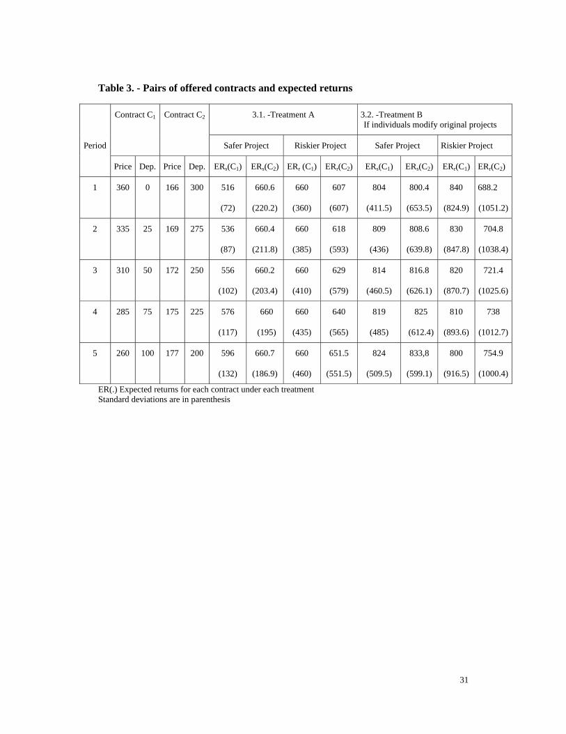
[INSERT TABLE 3]

Table 3 shows the pairs of contracts offered to the subjects in each period. The

pairs of contracts vary through periods, progressively decreasing the separation between

expected returns to test the sensitivity of different choices25. Table 3 also shows

Treatment A (described above) with which we test whether the pairs of contracts

designed, combining prices and security deposits, permit the separation of individuals

by their risk level. Chart 1 shows the contracts offered and the isoreturn curves that

provide the individuals with an expected return of 660. Any isoreturn curve above these

provides individuals with a lower expected return. The difference in the slopes reflects

our hypothesis that individuals with lower failure probability are inclined to accept a

higher increment in their security deposit for a given reduction in the asset price

compared with individuals with higher failure probability. If this hypothesis is accepted,

15

the security deposit (and asset price) can be used to separate individuals with a different

project risk. The contracts, hence, are designed to work as mechanisms to separate

different types of buyers.

[INSERT CHART 1]

In this experiment we consider, according to Bester (1985b), the pairs of

contracts offered to be incentive compatible because of their differences in the expected

returns for the individuals. Hence, we expect that the subjects with safer projects

choose Contract C2 and that the subjects with riskier projects prefer Contract C1.

However, if the subjects were risk averse, the incentive-compatibility of the contracts

should depend on the expected utility, as Bester (1987) notes. Therefore, the pair

expected return-standard deviation would determine subjects’ decisions. To prove this,

Table 4 shows the standard deviations of each of the contracts in each period. In this

case we still expect r subjects to prefer Contract C1.

All of the subjects, after making their decisions in Treatment A, read new

instructions for Treatment B. Under this treatment, moral hazard generated by ex ante

asymmetric information was introduced. This second treatment permits the comparison

of the same subjects’ decisions under two different environments (Treatment A and

Treatment B) in the same session. Thus, Treatment B allows us to test the effect of

moral hazard (generated by ex ante asymmetric information) on the effectiveness of

these contracts as a mechanism to separate borrowers with different risk levels. We

started within the same, previously described, context. The only change being that

subjects had the opportunity to make a second decision before learning about the

project’s success or failure. The second decision was whether to modify the original

project entailing an increase in the project probability of failure and expected return.

25 In the first session, we offered an initial "test" contract to make sure the subjects understood the instructions.

16

Under this treatment, moral hazard originated from the lack of control that sellers have

on the buyers’ project choice. Whenever the buyer was successful, he paid the contract

price. Consequently, moral hazard derived from the ex post asymmetric information

between buyers and sellers was excluded. The second treatment also contained several

periods in which each subject i = s, r was offered a pair of incentive compatible

contracts. Subjects chose one of these contracts or a risk-free investment, as in

Treatment A. The pairs of contracts were identical to those in Treatment A and

consequently the expected results, too, in case individuals did not modify original

projects. However, when individuals modified original projects, they also modified

their expected returns. The modified project of s individuals provided a return of 1,200

monetary units in case of success, with a probability of 0.6, and zero in case of failure.

Subjects r modifying the original projects had a success probability of 0.3 and obtained

a return of 2,160 monetary units; in case of failure the payoff was zero. Hence, the

expected return for each s and r subject for modifying the initial project was:

ERsm = 0.6 (300 + 1200 – Price) + 0.4 (300 + 0 – Deposit) (3)

ERrm = 0.3 (300 + 2160 – Price) + 0.7 (300 + 0 – Deposit)

Column 4.2 of Table 3 shows expected returns for each contract and each type of

subject in case they choose to change the original project. A situation was created in

which both types of individuals experienced an increase in their expected return if they

changed the original project. In each period, the type s subjects modifying their original

project reached an expected return with Contract C1 very close to that of Contract C2

which could lead them to decide to increase the risk of the project regardless of

choosing C1 or C2. On the other hand, subjects r modifying their original project had a

greater expected return with Contract C1 than with Contract C2. Hence, it was expected

17

that the subjects with riskier projects also increased the risk of their project and were

inclined to choose Contract C1.

This design was chosen for various reasons. First, real credit markets might

present this situation. Second, it is the case in which a higher moral hazard can be

generated, when both types of subjects may be interested in increasing the risk of their

original projects. In this case, sellers (lenders) might experience harm as they are

affected by the increase in project failure probability. The greater this probability, the

lower is the lender’s expected return. Finally, it makes it possible to observe whether

choices are guided by expected returns.

We are interested in testing Bester's (1987) hypothesis that contracts with higher

collateral have a positive incentive effect on the probability of repayment, making

projects with higher failure probability less attractive for borrowers. If this hypothesis

is verified in the experiments, the individuals that choose to increase the risk of the

project must choose Contract C1, with the lower security deposit. More specifically, to

verify hypothesis H2E , subjects s who choose to increase their project risk should

choose Contract C1 in Treatment B.

To control the possible incidence of the subjects’ risk aversion, we also calculate

the standard deviations in each of the contracts in each period when the original project

is modified, see Table 3. Individuals r obtain higher returns and lower standard

deviations with Contract C1 than with Contract C2 either when modifying the initial

contract or not. Moreover, modifying the initial project provides higher return and

higher standard deviation than non-modification. Hence, if the preferences of the

individuals were based on expected utility, subjects r are expected to choose Contract

C1, and it would be as rational to keep the original project as to change it. On the other

hand, s individuals have very similar expected returns with both contracts C1 and C2,

18

but a lower risk with Contract C1. In addition, changing the initial project results in

higher return and higher risk. Thus, if preferences are based on expected utility, our

expectation is that s individuals choose Contract C1 when modifying original projects.

Nevertheless, it is equally rational to modify the original project or not.

4.1. Experimental Procedures

We organized four experimental sessions with students of Universidad de

Valencia (Spain) and Washington and Lee University (USA) as subjects recruited from

various courses with flyers. There were 10 participants in each experimental session

except the second, which had 14 participants, no single subject participated in more than

one session. Each session lasted for one hour and 30 minutes and consisted of 10

periods. After privately assigning their types, riskier or safer, we read the instructions

and answered questions. The subjects, in each period, had an initial wealth of 300

monetary units and made their choices privately. During the experiment they were not

allowed to communicate with the rest of the participants and each subject only knew

their own project success and failure probabilities as well as their returns. After ending

the five periods of Treatment A, the subjects read instructions for the five periods of

Treatment B.26 At the end of the session we paid in cash each subject’s amount made

during five randomly chosen periods from Treatments A and B. Subjects made on

average $45.

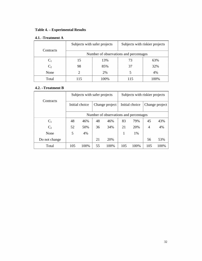
4.2. Results

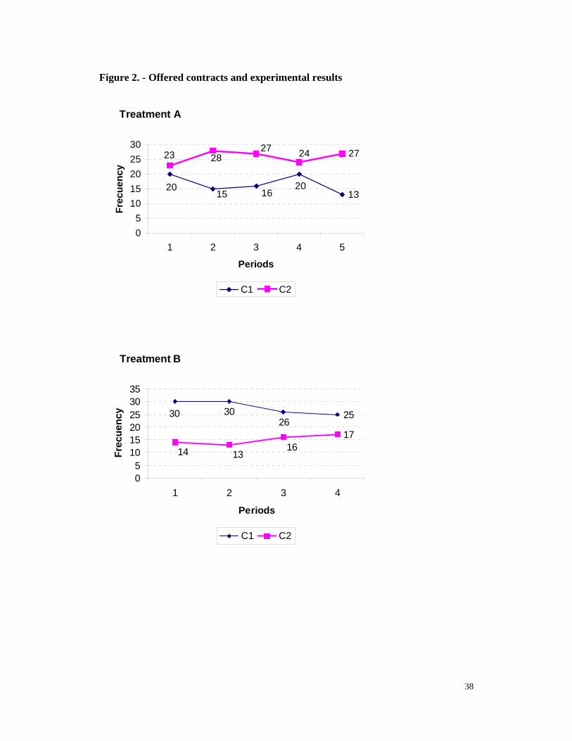
The results of the experiment are summarized in Table 4. There is a total of 440

observations; 230 correspond to Treatment A and 210 correspond to Treatment B. Half

of the subjects in the experiment had a riskier project and the other half had a safer

project. Chart 2 shows the distribution of the subjects' responses by treatment in each

26 The instructions and other documents used in this experiment are available upon request to the corresponding author.

19

period. The purpose of this experiment is to analyze whether offering a pair of incentive

compatible contracts combining collateral and interest rate requirements allows lenders

to separate borrowers according to their project risk, both without and with moral

hazard. In addition, we wanted to test whether this separating effect exceeds the

adverse selection and moral hazard effects of high collateral.

[INSERT TABLE 4]

[INSERT CHART 2]

Therefore, first the test of the separating power of contracts was run, similar to

the test of the combination collateral/interest rate in the previous section. The one

factor analysis of variance and the logit analysis were also used to examine the

experimental data.27 Contracts (CONTRACT variable) act as exogenous variable

because each contract has an incentive compatible combination of price and security

deposit. This test analyses whether the contract choice (C1 or C2) can be explained by

the project risk level with and without moral hazard. Then, the test of the influence of

moral hazard was run completing the analysis of the moral hazard influence on the

initial contract and the change of project choices.

4.2.1. Test of the Separating Power of Contracts

The variables used in this test are the following:

- Endogenous variable:

CONTRACT: Dummy variable that summarizes the information about collateral and

interest rates of a loan. Contract C1 is given value 0 and Contract C2 is given 1.

- Exogenous variables:

PROJECT: Dummy variable. Riskier projects r are given value 0 and safer ones s are

given value 1.

27 These logit analyses had no validation sample.

20

TREATMENT: Dummy variable. Treatment A (without moral hazard) is given value 0

and Treatment B (with moral hazard) is given value 1.

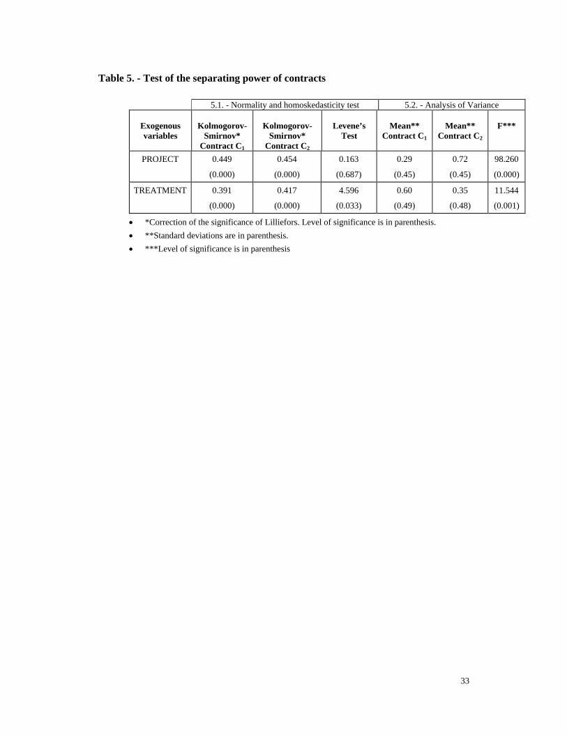
Results of the Analysis of Variance

Table 5 shows the ANOVA results28. Subjects with safer projects made most of

the C2 choices (72%). In contrast, subjects with riskier projects made most of the C1

choices, 71% of the total choices in the two treatments. Therefore, our hypothesis H1E

was proven right: by offering pairs of incentive compatible contracts, subjects with safer

projects chose Contract C2 and subjects with riskier projects chose Contract C1. On the

other hand, TREATMENT shows how choices change from Treatment A to Treatment

B. Contract C2 was chosen more frequently under Treatment A, without moral hazard

(65% of Contract C2 choices were under Treatment A). In contrast, Contract C1 was

chosen more often under Treatment B involving moral hazard (60% of Contract C1

choices were under Treatment B). The last column of Table 5.2 shows that the inter-

group differences are significant in both variables. The ANOVA results suggest that the

existence of moral hazard affects initial contract choices thus reducing the separating

effect of the incentive compatible contracts.

[INSERT TABLE 5]

Results of the Logit Analysis

Risk-free investment decisions were excluded from the total of the observed

subject choices in both treatments. Hence, we analyzed 427 choices, 219 of Contract C1

and 208 of Contract C2. The variable selection method was the forward stepwise

process of the likelihood ratio. Table 6 gives the results. PROJECT and

TREATMENT, were selected.

28 Normality and homogeneity of variance tests for each of the exogenous variables are also shown in Table 5. The two variables PROJECT and TREATMENT followed a distribution clearly different from normal, as expected. With respect to the homogeneity of variance, the null hypothesis of equal variances

21

[INSERT TABLE 6]

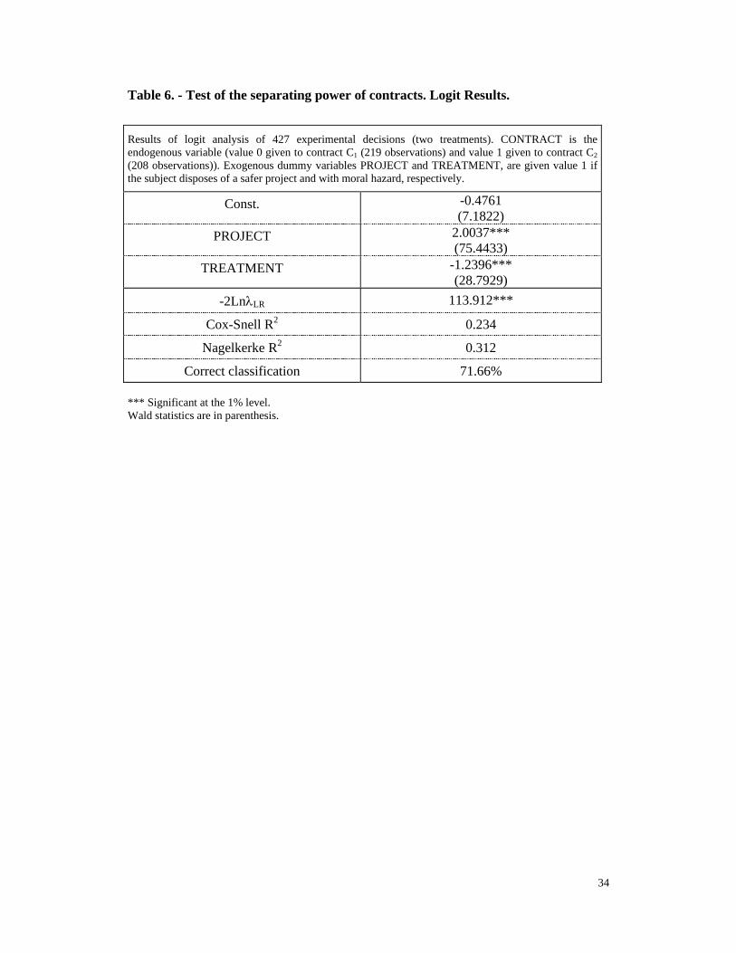
PROJECT indicates that the safer the project the greater the probability to

choose Contract C2. This result confirms the significance of the differences between

choices of subjects with safer projects and subjects with riskier projects. Hence, it is

ascertained that high collateral combined with an adequate low rate of interest attracts

principally subjects with safer projects. Moreover, this result suggests that in this

context high collateral does not generate adverse selection of borrowers. However, the

TREATMENT variable was also selected, i.e. Treatment B lowers the number of C2

choices compared with Treatment A, confirming the result of the analysis of variance.

Moral hazard alters initial contract choices thus reducing the separation effects of

incentive compatible contracts. With respect to the goodness of fit, Table 6 shows that

each of the coefficients is significantly different from zero. The two variables are

jointly significant when determining the probability of selecting Contract C2. Thus, the

chi-square with two degrees of freedom, −2 Ln LRλ , reaches 113.912 and a significance

level of 0.0000 which indicates that the null hypothesis according to which βj are both

zero must be rejected. In addition, a correct classification of 71.66% is obtained using

this function.

4.2.2. Test of the influence of moral hazard

The results in the previous test reveal the influence of moral hazard on initial

contract choices. This section extends those results by examining the differences in

borrowers’ choices according to their project risk. The endogenous variable is now the

dummy variable PROJECT. The differences between Group 1 (subjects with safer

projects) and Group 2 (subjects with riskier projects) are explained using the ANOVA

test based on the following exogenous variables:

in the two groups cannot be rejected. However, the lack of normality requires caution in the interpretation of the F of Snedecor.

22

CONTRACT(A): Contract choices in Treatment A. No contract choice was given value

0, Contract C1 choice was given value 1, and Contract C2 choice was given value 2.

CONTRACT(B): Contract choices in Treatment B. No contract choice was given value

0, Contract C1 choice was given value 1, and Contract C2 choice was given value 2.

CONTRACT(A+B): Contract choices in the two treatments globally. No contract

choice was given value 0, Contract C1 choice was given value 1, and Contract C2 choice

was given value 2.

INCREASE IN R: Subject’s second decision in Treatment B: to increase or not to

increase the risk level of the original project after choosing a contract. No modification

was given value 0, and while modifications were given value 1.

Results of the Analysis of Variance

Table 7 shows the ANOVA results29. CONTRACT(A) reveals a significant

difference in the contract choices of individuals with safer projects and those with

riskier projects. Most of the individuals with safer projects, 83%, chose Contract C2 in

Treatment A, which excludes the possibility of moral hazard. In contrast, most of the

individuals with riskier projects, 70%, chose Contract C1 in the same treatment.

[INSERT TABLE 7]

In Treatment B, 45% of individuals with safer projects chose Contract C2 and

most of the individuals with riskier projects, 81%, chose Contract C1. CONTRACT(B)

changes from a mean of 1.45 in Group 1 to a mean of 1.19 in Group 2, with a level of

significance of 0.000. However, though the difference in contract choices is significant,

it is lower than the one in Treatment A. It seems that moral hazard introduced in

Treatment B reduces the separating power of incentive compatible contracts. The joint

29 Table 7 also shows the results of normality and homogeneity of variance tests. CONTRACT(A+B) has the same variance in the two groups. The rest of exogenous variables do not observe the homogeneity of variance hypothesis required by the ANOVA. On the other hand, the four categorical exogenous variables follow a distribution different from normal.

23

exam of Treatments A y B shows that, globally, the differences in contract choices

between different risk level subjects is significant, as noticed in the test of the separating

power of contracts. Group 1 mean value of the CONTRACT(A+B) variable is 1.65

against a mean of 1.24 in Group 2, with a F of Snedecor’s level of significance of 0.000.

The results of the analysis of these three variables seem to confirm the effectiveness of

this menu of incentive compatible contracts in terms of expected returns to separate

borrowers according to their project risk level. Again, we do not find that a high

collateral requirement leads to an adverse selection of borrowers. In contrast, high

collateral appropriately combined with the interest rate attracts subjects with safer

projects. These results are consistent to the ones in section 2, obtained with data of real

markets. Moreover, we found that the separating effect of this menu of contracts exists

even in the moral hazard environment designed in Treatment B.

However, moral hazard generates an increase in the failure probability of the

projects once the loan is granted. Subjects with initially safer projects switch it and

increase the risk more often. This is shown by the differences in Group 1 and Group 2

mean values of INCREASE IN R. 79% of the decisions of subjects initially having a

safer project are to increase the failure probability, whereas only 47% of the decisions

of subjects with an originally riskier project switch. The F of Snedecor’s level of

significance indicates the hypothesis of equal means has to be rejected. Thus, moral

hazard results in the reduction of borrowers’ separation in two ways. First, the

proportion of Contract C2 choices of subjects with originally safer projects is reduced.

Second, some subjects with originally safer projects decide to increase the project

failure probability once the loan is granted. The Contract C2 choices in Treatment B (a

total of 73) change from 71% with safer projects to 22% after taking the decision of

increasing the project risk or not.

24

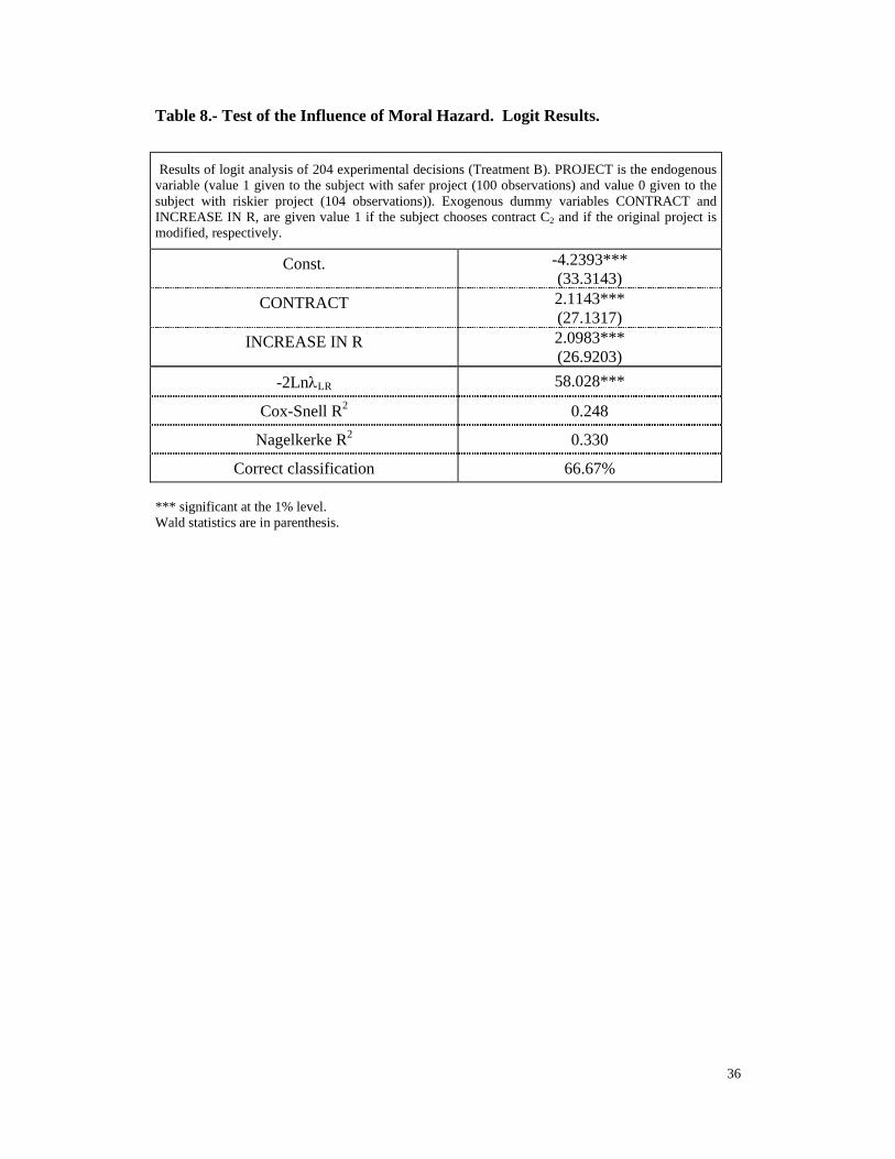
Results of the Logit Analysis

To verify the effects of moral hazard detected in the previous ANOVA a logit

analysis is run. We examine the project type of each subject (PROJECT), riskier or

safer, as a function of CONTRACT, representing the contract choice in Treatment B,

and INCREASE IN R, representing the decision to increase the probability of failure

after obtaining the loan. A logit analysis with the exogenous variable INCREASE IN R

requires limitation to Treatment B and exclusion of decisions without any contract

choices. In total 204 decisions were analyzed, 100 taken by subjects with safer projects

and 104 by subjects with riskier project. The method of variable selection is the

forward stepwise process of the likelihood ratio.

Table 8 shows that the two exogenous variables: CONTRACT(B) and

INCREASE IN R were selected in the final function. Contract C2 is more likely to be

chosen by a subject with a safer project. This variable clearly differentiates the

individuals with riskier projects from those with safer projects. Hence, the separating

effect of this menu of incentive compatible contracts remains, even in environments

where there is moral hazard. The selection of the variable INCREASE IN R indicates

that subjects with safer projects are more likely to increase their project risk once the

loan is granted, also shown in the previous analysis of variance. These results are fairly

robust. Table 8 shows that the coefficients of the two variables are far different from

zero. On the whole, these are also significant when differentiating contract choices,

since the chi-square with two degrees of freedom, −2 Ln LRλ , reaches a value of 58.028

and a level of significance of 0.0000, indicating that the null hypothesis according to

which the βj are all zeros, should be rejected. In addition, the percentage of correct

classification of choices is 66.67%.

[INSERT TABLE 8]

25

5. Conclusions

This paper examines the separating effect of collateral empirically by analyzing

data of real markets and of a controlled experiment, taking the role of moral hazard into

account. Such an analysis is suggested by the extant theories of the role of collateral in

credit markets with asymmetric information which assume that borrower preferences

among different combinations of interest and collateral systematically depend on their

risk levels. Empirical studies, so far, have been unable to examine the incentive

compatibility of this menu of contracts because individualized information on loan

contract features is unusual and does not include a direct and objective approximation to

the ex ante unobservable borrower risk.

First, we investigated the separating role of collateral by analyzing data

concerning a sample of credits to small and medium-sized firms guaranteed by the SGR

of Valencia, Spain. In contrast to other studies, we explored the combination

collateral/interest rate. Moreover, we used the real outcome of each loan as

approximation to the ex ante, i.e. privately known, borrower risk. Consistent with

previous papers, we found evidence that collateral is related to higher ex ante borrower

risk. Nevertheless, our results suggest that by combining collateral appropriately with

the interest rate, borrowers with different risk levels are separated and the borrowers

with higher risk tend to ask for loans without collateral and high interest rates.

Whereas, the borrowers with lower risk ask for loans with real asset collateral and low

interest rate. Hence, we provide first empirical evidence on the effectiveness of

collateral as a separating mechanism when it is adequately combined with interest rates.

Our results support the theoretical conclusions concerning collateral of Bester (1985b,

1987), Chan and Kanatas (1985), Besanko and Thakor (1987), Deshons and Freixas

(1987), Igawa and Kanatas (1990), Stiglitz and Weiss (1986, 1992), Boot, Thakor and

26

Udell (1991) and Coco (1999). Our results are also consistent with the assumption that

borrowers produce information about the ex ante borrower risk and indicate that lenders

systematically use this information to ask high-risk borrowers for higher collateral.

However, the evidence does not suggest that lenders use this information to ask a higher

interest rate from high-risk borrowers. Nevertheless, this empirical result must be

examined with caution as our data come from loans guaranteed by SGR’s. The lender

designs the terms of the contract given that the loan is secured by the SGR which, in

turn, analyzes the risk of the operation and decides whether to provide a guarantee and,

if so, what level of collateral is requested.

Experimental data involving relatively simple decisions in a controlled setting

also support previous results of our empirical analysis in real credit markets. However,

our experimental results show the existence of moral hazard that reduce the efficacy of

incentive compatible contracts in separating borrowers according to their risk levels.

Moreover, in contrast to Bester (1987), we find no positive incentive effects of contracts

with high collateral. Indeed, we find that contracts with high collateral do not make

subjects less likely to increase the probability of failure of their projects in an

environment with moral hazard.

References

Allen (1983)

Benjamin (1978)

Berger, A. N., and Udell, G. F., 1990. Collateral, loan quality and bank risk. Journal of Monetary

Economics 25, 21-42.

Besanko, D., and Thakor, A., 1987. Collateral and rationing: sorting equilibria in monopolistic and

competitive credit markets. International Economic Review 28, 3, 671-689.

Bester, H., 1985a. The level of investment in credit markets with imperfect information. Journal of

Institutional and Theoretical Economics 141, 503-515.

27

Bester, H., 1985b. Screening vs. rationing in credit markets with imperfect information. American

Economic Review 75, 4, 850-855.

Bester, H., 1987. The role of collateral in credit markets with imperfect information. European

Economic Review 31, 887-899.

Boot, A. W. A., Thakor, A. V., and Udell, G. F., 1991. Secured lending and default risk: Equilibrium

analysis and policy implications and empirical results. Economic Journal 101, 458-472.

Brennan, M., and Kraus, A., 1987. Efficiency financing under asymmetric information. Journal of

Finance 42, 5, 1225-1243.

Cabrer, B., Sancho, A., and Serrano, G., 2001. Microeconometría y decisión. Pirámide, Madrid.

Chan, Y. S., and Kanatas, G., 1985. Asymmetric valuations and the role of collateral in loan agreements.

Journal of Money, Credit and Banking, 84-95.

Coco, G., 1999. Collateral, heterogeneity in risk attitude and the credit market equilibrium. European

Economic Review 43, 559-574.

Deshons, M., and Freixas, X., 1987. Le rôle de la garantie dans les contrats de prêt bancaire. Finance 8,

1, 7-32.

Grinblatt, M., and Hwang, C. Y., 1989. Signaling and the pricing of new issues. Journal of Finance 44,

2, 393-420.

Hester, D., 1979. Customer relationships and terms of loans: Evidence from a pilot survey. Journal of

Money, Credit and Banking 11, 349-357.

Igawa, K., and Kanatas, G., 1990. Asymmetric information, collateral, and moral hazard. Journal of

Financial and Quantitative Analysis 25, 4, 469-490.

Jaffe y Russell (1976)

Leeth, J. D., and Scott, J. A., 1989. The incidence of secured debt: evidence from the small business

community. Journal of Financial and Quantitative Analysis 24, 3, 379-394.

Leland, H. E., and Pyle, D. H., 1977. Informational Asymmetries, financial structure and financial

intermediation. Journal of Finance 32, 371-387.

Machauer, A., and Weber, M., 1998. Bank behavior based on internal credit ratings of borrowers.

Journal of Banking and Finance 22, 1355-1383.

Milde, H., and Riley, J., 1988. Signaling in credit markets. Quarterly Journal of Economics 103, 101-

129.

28

Orgler, Y., 1970. A credit scoring model for commercial loans. Journal of Money, Credit and Banking 2,

435-445.

Ramírez Comeig, I., and Ferrando Bolado, 1999. La Sociedad de Garantía Recíproca de la Comunidad

Valenciana. Análisis y evolución 1982-1998. Sociedad de Garantía Recíproca de la Comunidad

Valenciana, Valencia.

Rostchild y Stiglitz (1970)

Stiglitz, J. E., and Weiss, A., 1981. Credit rationing in markets with imperfect information. American

Economic Review 71, 3, 393-410.

Stiglitz, J. E., and Weiss, A., 1986. Credit rationing and collateral, in: Edwards, J., Franks, J., Mayer, C.,

Schaefer, S. (Eds.), Recent developments in Corporate Finance, Cambridge University Press, New

York, pp. 101-135.

Stiglitz, J. E., and Weiss, A., 1992. Asymmetric information in credit markets and its implications for

macro-economics. Oxford Economic Papers 44, 694-724.

Uriel, E., 1995. Análisis de datos: series temporales y análisis multivariante. AC, Madrid.

Wette, H., 1983. Collateral in credit rationing in markets with imperfect information. American

Economic Review 73, 3, 442-445.

29

Table 1. - Test of the combination collateral-interest rate.

1.1. - Normality and homoskedasticity test 1.2. - Analysis of Variance

Exogenous variables

Kolmogorov-

Smirnov* Contract C2

Kolmogorov-

Smirnov* Contract C1

Levene’s

Test

Mean**

Contract C2

Mean**

Contract C1

F***

FIRMTYPE 0.277

(0.000)

0.332

(0.000)

37.681

(0.000)

0.86

(0.67)

1.25

(0.86)

20.181

(0.000)

FIRMTYPE(1) 0.439

(0.000)

0.454

(0.000)

1.398

(0.238)

0.31

(0.46)

0.28

(0.45)

0.347

(0.556)

FIRMTYPE(2) 0.353

(0.000)

0.491

(0.000)

95.316

(0.000)

0.52

(0.50)

0.20

(0.40)

40.61

(0.000)

EMPL 0.270

(0.000)

0.197

(0.000)

46.940

(0.000)

17.39

(28.31)

40.39

(43.61)

32.08

(0.000)

SIZE 0.152

(0.000)

0.209

(0.000)

11.066

(0.001)

20,314.76

(14,756.79)

11,666.12

(12,481.,76)

31.712

(0.000)

TERM 0.318

(0.000)

0.154

(0.000)

27.274

(0.00)

80.51

(18.8)

46.99

(22.0)

213.944

(0.000)

DEST 0.520

(0.000)

0.541

(0.000)

36.775

(0.000)

0.87

(0.34)

0.96

(0.20)

8.234

(0.004)

OUTC 0.536

(0.000)

0.434

(0.000)

573.073

(0.000)

0.98

(0.13)

0.68

(0.47)

64.432

(0.000)

• EMPL: number of employees per firm; SIZE: amount granted in thousands of pesetas; TERM: term of the loan in months. The rest are dummy variables.

• *Correction of the significance of Lilliefors . Level of significance is in parenthesis. • **Standard deviations are in parenthesis. • ***Level of significance is in parenthesis

30

Table 2. Test of the combination collateral - interest rate. Logit Results.

The estimation sample consists of 303 loans to small and medium-sized firms guaranteed by SGR of Land of Valencia from 1983 to 1998. CONTRACT is the endogenous variable (value 1 given to contract C1 (172 observations) and value 0 given to contract C2 (131 observations). Exogenous dummy variables FIRMTYPE(1), FIRMTYPE(2), DEST and OUTC are given value 1 in the case of sole proprietors, PLCs., investments not corresponding to the set-up of a new company and in case of non-repayment, respectively. Variables SIZE and TERM, in pesetas and months, respectively.

Const. 6.2632*** (25.7214)

FIRMTYPE(1) -1.8117*** (9.2702)

FIRMTYPE(2) -2.3273*** (19.9488)

EMPL 0.0285*** (18.5548)

SIZE -7.2E-08*** (12.8514)

TERM -0.0697*** (39.8156)

DEST 2.2157*** (9.0362)

OUTC -2.5857*** (9.6724)

-2LnλLR 238.690***

Cox-Snell R2 0.545

Nagelkerke R2 0.731

Correct classification 89.11% of estimation sample

100% of validation sample *** Significant at the 1% level. Wald statistics are in parenthesis.

31

Table 3. - Pairs of offered contracts and expected returns

3.1. -Treatment A 3.2. -Treatment B If individuals modify original projects

Contract C1 Contract C2

Safer Project Riskier Project Safer Project Riskier Project Period

Price Dep. Price Dep. ERs(C1) ERs(C2) ERr (C1) ERr(C2) ERs(C1) ERs(C2) ERr(C1) ERr(C2)

1 360 0 166 300 516

(72)

660.6

(220.2)

660

(360)

607

(607)

804

(411.5)

800.4

(653.5)

840

(824.9)

688.2

(1051.2)

2 335 25 169 275 536

(87)

660.4

(211.8)

660

(385)

618

(593)

809

(436)

808.6

(639.8)

830

(847.8)

704.8

(1038.4)

3 310 50 172 250 556

(102)

660.2

(203.4)

660

(410)

629

(579)

814

(460.5)

816.8

(626.1)

820

(870.7)

721.4

(1025.6)

4 285 75 175 225 576

(117)

660

(195)

660

(435)

640

(565)

819

(485)

825

(612.4)

810

(893.6)

738

(1012.7)

5 260 100 177 200 596

(132)

660.7

(186.9)

660

(460)

651.5

(551.5)

824

(509.5)

833,8

(599.1)

800

(916.5)

754.9

(1000.4)

ER(.) Expected returns for each contract under each treatment Standard deviations are in parenthesis

32

Table 4. – Experimental Results

4.1. -Treatment A

Subjects with safer projects Subjects with riskier projects

Contracts Number of observations and percentages

C1 15 13% 73 63% C2 98 85% 37 32%

None 2 2% 5 4%

Total 115 100% 115 100%

4.2. –Treatment B

Subjects with safer projects Subjects with riskier projects

Initial choice Change project Initial choice Change project

Contracts

Number of observations and percentages

C1 48 46% 48 46% 83 79% 45 43% C2 52 50% 36 34% 21 20% 4 4%

None 5 4% 1 1%

Do not change 21 20% 56 53%

Total 105 100% 55 100% 105 100% 105 100%

33

Table 5. - Test of the separating power of contracts

5.1. - Normality and homoskedasticity test 5.2. - Analysis of Variance

Exogenous variables

Kolmogorov-

Smirnov* Contract C1

Kolmogorov-

Smirnov* Contract C2

Levene’s

Test

Mean**

Contract C1

Mean**

Contract C2

F***

PROJECT 0.449

(0.000)

0.454

(0.000)

0.163

(0.687)

0.29

(0.45)

0.72

(0.45)

98.260

(0.000)

TREATMENT 0.391

(0.000)

0.417

(0.000)

4.596

(0.033)

0.60

(0.49)

0.35

(0.48)

11.544

(0.001)

• *Correction of the significance of Lilliefors. Level of significance is in parenthesis. • **Standard deviations are in parenthesis. • ***Level of significance is in parenthesis

34

Table 6. - Test of the separating power of contracts. Logit Results.

Results of logit analysis of 427 experimental decisions (two treatments). CONTRACT is the endogenous variable (value 0 given to contract C1 (219 observations) and value 1 given to contract C2 (208 observations)). Exogenous dummy variables PROJECT and TREATMENT, are given value 1 if the subject disposes of a safer project and with moral hazard, respectively.

Const. -0.4761 (7.1822)

PROJECT 2.0037*** (75.4433)

TREATMENT -1.2396*** (28.7929)

-2LnλLR 113.912***

Cox-Snell R2 0.234

Nagelkerke R2 0.312

Correct classification 71.66% *** Significant at the 1% level. Wald statistics are in parenthesis.

35

Table 7. – Test of the Influence of Moral Hazard

7.1. - Normality and homoskedasticity test 7.2. - Analysis of Variance

Exogenous variables

Kolmogorov-

Smirnov* Group 1

Safer projects

Kolmogorov-

Smirnov* Group 2

Riskier projects

Levene’s

Test

Mean** Group 1

Safer projects

Mean** Group 2 Riskier projects

F***

CONTRACT(A) 0.506 (0.000)

0.375 (0.000)

23.025 (0.000)

1.83 (0.42)

1.28 (0.54)

76.674 (0.000)

CONTRACT(B) 0.321 (0.000)

0.476 (0.000)

46.495 (0.000)

1.45 (0.59)

1.19 (0.42)

13.334 (0.000)

CONTRACT(A+B) 0.423 (0.000)

0.423 (0.000)

8.951 (0.003)

1.65 (0.54)

1.24 (0.49)

72.211 (0.000)

INCREASE IN R 0.486 (0.000)

0.355 (0.000)

50.397 (0.000)

0.79 (0.41)

0.47 (0.50)

24.632 (0.000)

• *Correction of the significance of Lilliefors . Level of significance is in parenthesis. • **Standard deviations are in parenthesis. • ***Level of significance is in parenthesis

36

Table 8.- Test of the Influence of Moral Hazard. Logit Results.

Results of logit analysis of 204 experimental decisions (Treatment B). PROJECT is the endogenous variable (value 1 given to the subject with safer project (100 observations) and value 0 given to the subject with riskier project (104 observations)). Exogenous dummy variables CONTRACT and INCREASE IN R, are given value 1 if the subject chooses contract C2 and if the original project is modified, respectively.

Const. -4.2393*** (33.3143)

CONTRACT 2.1143*** (27.1317)

INCREASE IN R 2.0983*** (26.9203)

-2LnλLR 58.028***

Cox-Snell R2 0.248

Nagelkerke R2 0.330

Correct classification 66.67% *** significant at the 1% level. Wald statistics are in parenthesis.

37

Figure 1. - Treatment A. Offered contracts and isoreturn curves.

Expected Return = 660

050

100150200250300350400

0 50 100 150 200 250 300 350

Security Deposit

Pric

e

Safer Project Riskier Project

38

Figure 2. - Offered contracts and experimental results

Treatment A

13

27

2015 16

20

2723 28 24

05

1015202530

1 2 3 4 5

Periods

Frec

uenc

y

C1 C2

Treatment B

25

17

30 3026

14 1316

05

101520253035

1 2 3 4

Periods

Frec

uenc

y

C1 C2