Revised: April 1, 1997

More than a Dozen Alternative Ways of Spelling Gini1

by

Shlomo Yitzhaki

ABSTRACT

This paper surveys alternative ways of expressing the Gini mean difference and the Gini coefficient.

It adds some new representations and new interpretations of Gini's mean difference and the Gini

coefficient. All in all, there are over a dozen alternative ways of writing the Gini, which can be

useful in developing applications to Gini-based statistics.

Mailing Address:

Department of Economics Hebrew University Jerusalem, 91905 Israel E-Mail – shlomo.yitzhaki@huji.ac.il Source: Yitzhaki, S.: More than a Dozen Alternative Ways of Spelling Gini, Research on

Economic Inequality. 8, 1998, 13-30.

1 I would like to thank Peter Lambert for very helpful comments and a reference the Gini's original work in English.

More than a Dozen Alternative Ways of Spelling Gini

Gini's mean difference (GMD) as a measure of variability has been known for over a century.2 It

was `rediscovered' several times (see, for example, David, 1968; Jaeckel, 1972; Jurečková, 1969;

Olkin and Yitzhaki, 1992; Simpson, 1948) which means that it had been used by investigators who

did not know that they were using a statistic, which was a version of the GMD. One possible

explanation of this phenomenon is the large number of seemingly unrelated presentations of the

Gini's mean difference (and other statistics that are derived from it), which makes it hard to identify

which Gini one is dealing with. Being able to identify a Gini enables the investigator to derive

additional properties of the statistic at hand and rewrite it in an alternative, more user-friendly way.

It also enables the investigator to find new interpretations of the Gini and of Gini- related statistics.

One must be familiar with alternative definitions whenever one is interested in extension of the

statistics at hand: as will become obvious later, some definitions are more amenable to such

extension. Unfortunately, the alternative representations are scattered throughout many papers,

spread over a long period and many areas of interest, and are not readily accessible.3

2 For a description of its early development - see Dalton (1920); David (1981, p. 192); Gini (1921, 1936), and several entries in Harter (1978). Unfortunately, I am unable to survey the Italian literature, which includes, among others, Gini's (1912) original presentation of the index. A comprehensive survey of this literature can be found in Giorgi (1990, 1993).

3This phenomenon seems to be a characteristic of the literature on the GMD from its early development. Gini (1921) argues " Probably these papers have escaped Mr. Dalton's attention owing to the difficulty of access to the publications in which they appeared." (Gini, 1921, p. 124).

The aim of this paper is to survey alternative presentations of the GMD. As the survey is

restricted to quantitative random variables, the literature on diversity, which is mainly concerned

with categorical data, is not covered.4 For some purposes, the continuous formulation is more

convenient, yielding insights that are not as accessible when the random variable is discrete. The

continuous formulation is also preferred because it can be handled using calculus.5 To avoid

problems of existence, only continuous distributions with finite first moment will be considered.

The presentation is also restricted to population parameters, ignoring different types of estimators. It

is assumed that sample values substitute for population parameters in the estimation. As far as I

know, these alternative representations cover all known cases but I would not be surprised if others

turn up. The different formulations explain why the GMD can be applied in so many different fields

and given so many different interpretations.

The Gini coefficient is the GMD divided by twice the mean income. Actually, it is the most

well-known member of the Gini family and it is mainly used to measure income inequality. The

relationship between the two is similar to that between variance and the coefficient of variation.

Hence, one need only derive the GMD, and then easily convert the representation into a Gini

coefficient. Some additional properties relevant to the Gini coefficient will be added later. It is

worth mentioning that reference to "variability" or "risk" (most common among statisticians and

4For use of the GMD in categorical data, see the bibliography in Rao (1982) and Dennis et al. (1979) in biology, Lieberson (1969) in sociology; Bachi (1956) in linguistic homogeneity , and Gibbs and Martin (1962) for industry diversification.

5 One way of writing the Gini is based on vectors and matrices. This form is clearly restricted to discrete variables and hence it is not covered in this paper. For a description of the method see Silber (1989).

finance specialists) implies use of the Gini mean difference (GMD), whereas reference to

"inequality" (usually in the context of income distribution) implies use of Gini coefficient. The

difference is not purely semantic or even one of plain arithmetic: it reveals a distinction in one's

definition of an increase in variability (inequality). To see the difference, consider a distribution

bounded by [a,b] and ask what is the most variable (unequal) distribution. If the most variable

distribution is defined as the one with half of the population at a and the other half at b then the

GMD (or the variance) is the appropriate index of variability. If the most unequal distribution is

defined as the one with almost all the population concentrated at a and a tiny fraction at b, (all

income in the hand of one person), then the appropriate index is the Gini coefficient (or the

coefficient of variation).

The structure of the paper is as follows: The next section derives the alternative

presentations of the GMD; the third section adds some properties specific to the Gini coefficient.

The fourth section investigates the similarity with variance. The paper concludes with a section

indicating areas of further research.

2. Alternative Presentations of GMD

There are four types of formulae for GMD, depending on the elements involved. The first type is

based on absolute values, the second relies on integrals of cumulative distributions, the third on

covariances, and the forth on Lorenz curves (or integrals of first moment distributions).

Let X1, X2 be i. i. d. continuous random variables with F(x) representing the cumulative

distribution and f(x) the density function. It is assumed that the expected value, µ, exists; hence

limt→-∞ tF(t) = limt→∞ t[1-F(t)] = 0.

2.a: Formulations based on absolute values

The original definition of the GMD is the expected difference between two realizations of i.i.d.

variables. That is, the GMD in the population is:

Γ = E {|X1 - X2|} , (1)

which can be given the following interpretation: Consider an investigator who is interested in

measuring the variability of a certain property in the population. He draws a random sample of two

observations and records the difference between them. Repeating the sampling and averaging the

differences an infinite number of times yields the GMD.6 Hence, the GMD can be interpreted as the

expected difference between two randomly drawn members of the population.

A variant of (1) is:

Γ = E { E{|X1 - q|}|q = X2} . (2)

The term E{X1 - q} is the absolute deviation of X1 from q, where q is a quantile of X. The GMD is

therefore the expected value of absolute deviations from quantiles of the random variable. In other

words, the GMD is the average value of all possible absolute deviations of a variable from itself.

A slightly different set of presentations relies on the following identities: Let x, y be two

variables. then

6 See also Pyatt (1976) for an interesting interpretation based on a view of the Gini coefficient as the equilibrium of a game.

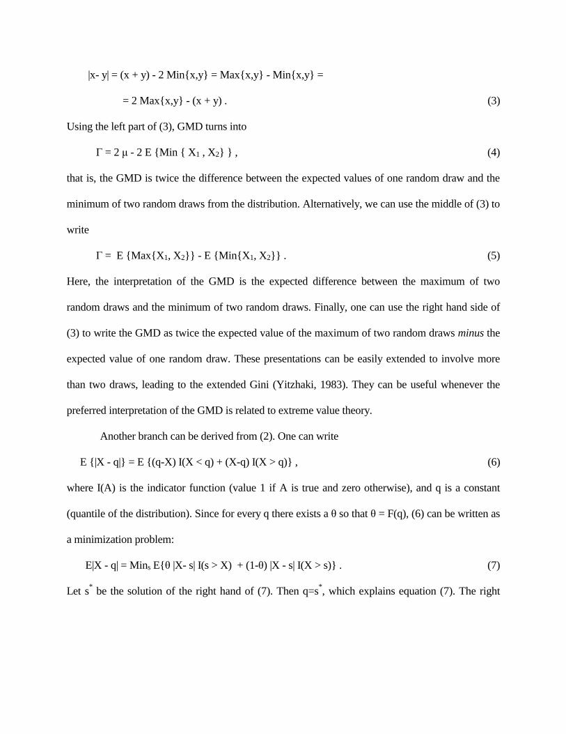
|x- y| = (x + y) - 2 Min{x,y} = Max{x,y} - Min{x,y} =

= 2 Max{x,y} - (x + y) . (3)

Using the left part of (3), GMD turns into

Γ = 2 µ - 2 E {Min { X1 , X2} } , (4)

that is, the GMD is twice the difference between the expected values of one random draw and the

minimum of two random draws from the distribution. Alternatively, we can use the middle of (3) to

write

Γ = E {Max{X1, X2}} - E {Min{X1, X2}} . (5)

Here, the interpretation of the GMD is the expected difference between the maximum of two

random draws and the minimum of two random draws. Finally, one can use the right hand side of

(3) to write the GMD as twice the expected value of the maximum of two random draws minus the

expected value of one random draw. These presentations can be easily extended to involve more

than two draws, leading to the extended Gini (Yitzhaki, 1983). They can be useful whenever the

preferred interpretation of the GMD is related to extreme value theory.

Another branch can be derived from (2). One can write

E {|X - q|} = E {(q-X) I(X < q) + (X-q) I(X > q)} , (6)

where I(A) is the indicator function (value 1 if A is true and zero otherwise), and q is a constant

(quantile of the distribution). Since for every q there exists a θ so that θ = F(q), (6) can be written as

a minimization problem:

E|X - q| = Mins E{θ |X- s| I(s > X) + (1-θ) |X - s| I(X > s)} . (7)

Let s* be the solution of the right hand of (7). Then q=s*, which explains equation (7). The right

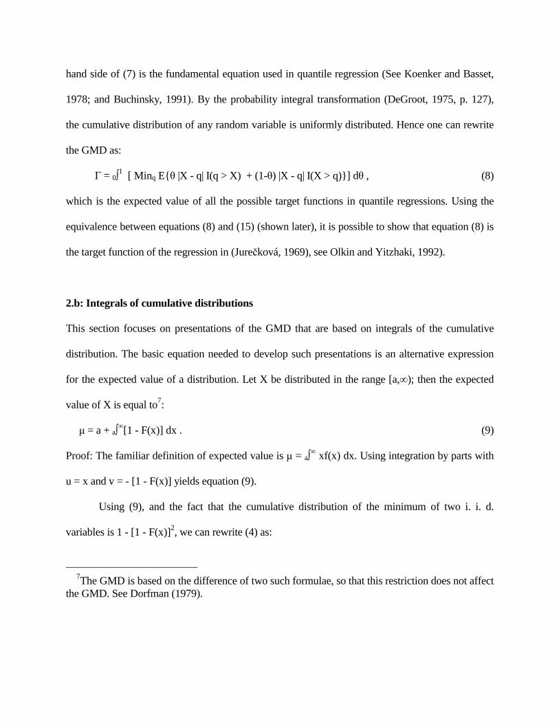
hand side of (7) is the fundamental equation used in quantile regression (See Koenker and Basset,

1978; and Buchinsky, 1991). By the probability integral transformation (DeGroot, 1975, p. 127),

the cumulative distribution of any random variable is uniformly distributed. Hence one can rewrite

the GMD as:

Γ = 0∫1 [ Minq E{θ |X - q| I(q > X) + (1-θ) |X - q| I(X > q)}] dθ , (8)

which is the expected value of all the possible target functions in quantile regressions. Using the

equivalence between equations (8) and (15) (shown later), it is possible to show that equation (8) is

the target function of the regression in (Jurečková, 1969), see Olkin and Yitzhaki, 1992).

2.b: Integrals of cumulative distributions

This section focuses on presentations of the GMD that are based on integrals of the cumulative

distribution. The basic equation needed to develop such presentations is an alternative expression

for the expected value of a distribution. Let X be distributed in the range [a,∞); then the expected

value of X is equal to7:

µ = a + a∫∞[1 - F(x)] dx . (9)

Proof: The familiar definition of expected value is µ = a∫∞ xf(x) dx. Using integration by parts with

u = x and v = - [1 - F(x)] yields equation (9).

Using (9), and the fact that the cumulative distribution of the minimum of two i. i. d.

variables is 1 - [1 - F(x)]2, we can rewrite (4) as:

7The GMD is based on the difference of two such formulae, so that this restriction does not affect the GMD. See Dorfman (1979).

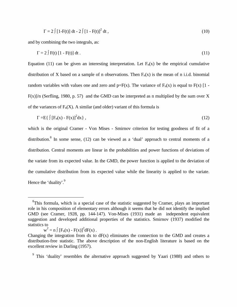
Γ = 2 ∫ [1-F(t)] dt - 2 ∫ [1 - F(t)]2 dt , (10)

and by combining the two integrals, as:

Γ = 2 ∫ F(t) [1 - F(t)] dt . (11)

Equation (11) can be given an interesting interpretation. Let Fn(x) be the empirical cumulative

distribution of X based on a sample of n observations. Then Fn(x) is the mean of n i.i.d. binomial

random variables with values one and zero and p=F(x). The variance of Fn(x) is equal to F(x) [1 -

F(x)]/n (Serfling, 1980, p. 57) and the GMD can be interpreted as n multiplied by the sum over X

of the variances of Fn(X). A similar (and older) variant of this formula is

Γ =E{ ∫ [Fn(x) - F(x)]2dx} , (12)

which is the original Cramer - Von Mises - Smirnov criterion for testing goodness of fit of a

distribution.8 In some sense, (12) can be viewed as a ‘dual’ approach to central moments of a

distribution. Central moments are linear in the probabilities and power functions of deviations of

the variate from its expected value. In the GMD, the power function is applied to the deviation of

the cumulative distribution from its expected value while the linearity is applied to the variate.

Hence the ‘duality’.9

8This formula, which is a special case of the statistic suggested by Cramer, plays an important role in his composition of elementary errors although it seems that he did not identify the implied GMD (see Cramer, 1928, pp. 144-147). Von-Mises (1931) made an independent equivalent suggestion and developed additional properties of the statistics. Smirnov (1937) modified the statistics to w2 = n ∫ [Fn(x) - F(x)]2dF(x) . Changing the integration from dx to dF(x) eliminates the connection to the GMD and creates a distribution-free statistic. The above description of the non-English literature is based on the excellent review in Darling (1957).

9 This ‘duality’ resembles the alternative approach suggested by Yaari (1988) and others to

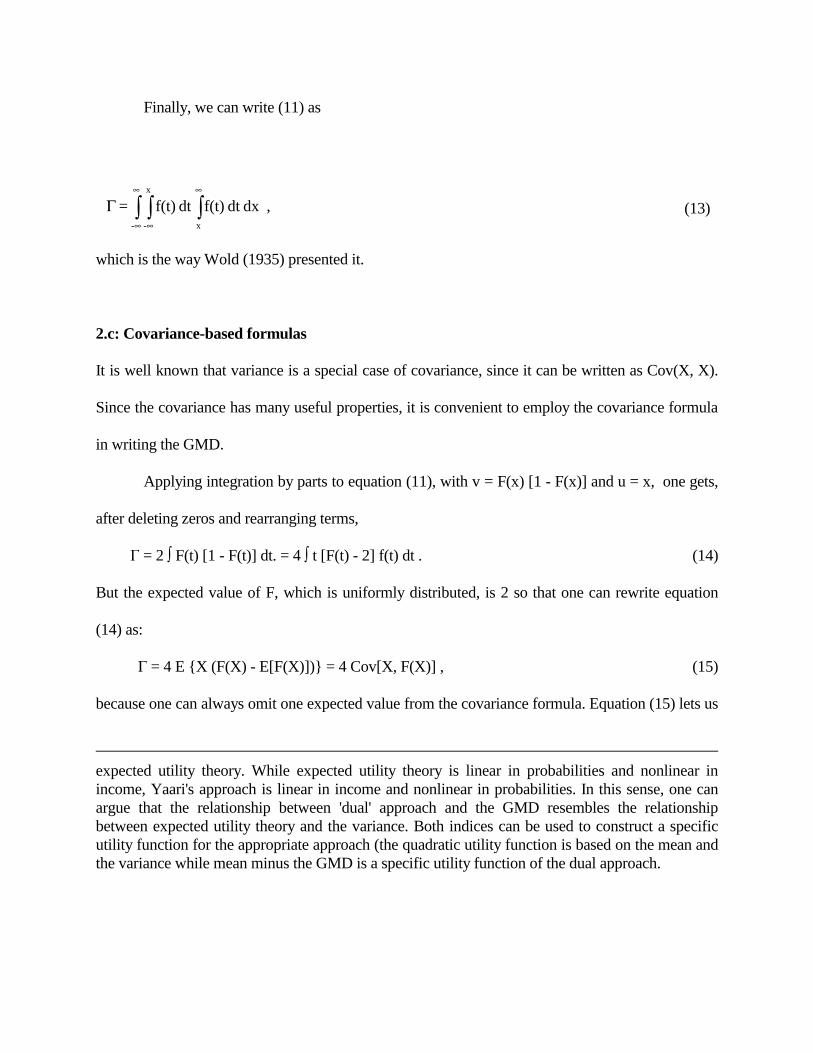
Finally, we can write (11) as

which is the way Wold (1935) presented it.

2.c: Covariance-based formulas

It is well known that variance is a special case of covariance, since it can be written as Cov(X, X).

Since the covariance has many useful properties, it is convenient to employ the covariance formula

in writing the GMD.

Applying integration by parts to equation (11), with v = F(x) [1 - F(x)] and u = x, one gets,

after deleting zeros and rearranging terms,

Γ = 2 ∫ F(t) [1 - F(t)] dt. = 4 ∫ t [F(t) - 2] f(t) dt . (14)

But the expected value of F, which is uniformly distributed, is 2 so that one can rewrite equation

(14) as:

Γ = 4 E {X (F(X) - E[F(X)])} = 4 Cov[X, F(X)] , (15)

because one can always omit one expected value from the covariance formula. Equation (15) lets us

expected utility theory. While expected utility theory is linear in probabilities and nonlinear in income, Yaari's approach is linear in income and nonlinear in probabilities. In this sense, one can argue that the relationship between 'dual' approach and the GMD resembles the relationship between expected utility theory and the variance. Both indices can be used to construct a specific utility function for the appropriate approach (the quadratic utility function is based on the mean and the variance while mean minus the GMD is a specific utility function of the dual approach.

, dxdt f(t)dt f(t) = x

x

--∫∫∫∞

∞

∞

∞

Γ (13)

calculate the GMD using a simple regression program.10 Since by definition Cov[F(X), F(X)] =

1/12 (because it is the variance of a uniformly distributed variable) we can write the GMD as

Γ = (1/3) Cov[X,F(X)]/ Cov [F(X), F(X)] , (16)

which can be given the following interpretation: Assume that the observations are arrayed in

ascending order, (say, by height as in the case of soldiers on parade), with equal distance between

each two observations (soldiers). The following proposition summarizes two interpretations of the

GMD:

Proposition 1:

(a) The GMD is equal to one third of the slope of the regression curve of the variable observed

(height) as a function of each observation's position in the array.

(b) The GMD is a weighted average of the differences in, say, heights between adjacent soldiers

(alternatively, it is a weighted average of the slopes defined by each two adjacent heights in the

array). The weights are symmetric around the median, with the median having the highest weight.

Proof of (a)

Let X(p) be the height of each soldier as a function of its position, p. Note that X(p) is the inverse of

the cumulative distribution of X. Using Ordinary Least Squares, the slope of heights is defined as

10 See Lerman and Yitzhaki (1984) for the derivation and interpretation of the formula, Jenkins (1987) on actual calculations using available software, and Lerman and Yitzhaki (1989) on using this equation to calculate the GMD in stratified samples. As far as I know, Stuart (1954) was the first to notice that the GMD can be written as a covariance. However, his findings were confined to normal distributions. Pyatt, Chau-nan, and Fei (1980) also write the Gini coefficient as a covariance. Hart (1975) argues that the moment-generating function was at the heart of the debate between Corardo Gini and Western statisticians. Hence, it is a bit ironic to find that one can write the GMD as some kind of a central moment.

COV(X,p)/COV(p,p). Since p is uniformly distributed, cov(p,p) = 1/12, which completes the proof

of (a).

Proof of (b):

Writing explicitly the numerator in (16) we get cov(x,p) = ∫ x(p) (p - 2) dp and by using integration

by parts with u=x(p) and v = (p - 2)2/2 we get:

cov(X,p) = x(p) (p-2)2/2|10 - 2 ∫ x'(p) (p - 2)2 dp .

Substituting x(1) - x(0) = ∫x'(p)dp, where x' denote a derivative, we get

cov(X,p) = 2 ∫ x'(p) p(1-p) dp . (17)

The GMD is equal to the weighted average of the slopes between the heights of each adjacent pair

of soldiers; the weighting scheme is symmetric in ranking around the median, and the farther away

each pair of soldiers from the middle of the distribution -- the lower the weight assign to their slope.

Since X(p) is the inverse of the cumulative distribution it is easy to see that X'(p) = 1/f(x), that is,

the reciprocal of the density function. Hence, a consequence of (17) is that the lower the density

function the larger the GMD. To sum up, according to these presentations, the GMD is the average

change in a variable for a small change in rank.

Equation (15), the covariance formula of the GMD, can be used to show that R-regressions

[Hettmansperger, (1984)] are actually based on minimizing the GMD of the error term. To see that,

note that the target function in R-regression is to minimize ∑i ei R(ei), where ei is the error term of

observation i in the regression while R(ei) is the rank of the error term. Keeping in mind that the

mean of the error term is constrained to equal zero, and that the rank is the empirical representation

of the cumulative distribution will lead us to the conclusion that R-regression are actually based on

minimizing the GMD of the error term. Then, some properties of these regressions can be traced to

the properties of the GMD.

2.d: Lorenz-Curve-based formulas

The fourth set of presentations of the GMD is based on the generalized Lorenz Curve (GLC),

which is also referred to as the absolute concentration curve.11 There are several definitions of this

curve. We follow Gastwirth's (1971, 1972) definition, which is based on the inverse of the

cumulative distribution x(p): p is plotted on the horizontal axis while the vertical axis represents the

cumulative value of the variate, -∞∫p x(t)dt. The familiar Lorenz curve is derived from the GLC by

dividing the cumulative value of the variate by the mean: the vertical axis is then (1/µ), -∞∫p x(t)dt.

The GLC has the following properties:

1. The GLC passes through (0,0) and (1,µ). The Lorenz curve passes through (0,0) (1,1).

2. The derivative of the curve at p is x(p); hence the curve is increasing (decreasing) depending on

whether x is negative (positive).

Figure 1 presents a typical GLC, the curve OAB. Before proceeding with the relationship

between the GLC and the GMD, I discuss some geometrical properties of the curve. The slope of

the line connecting the two extremes of the curve is µ. I refer to this line as the Line of Equality

11 The term "generalized Lorenz curve" was coined by Shorrocks (1983). Lambert (1993) gives an excellent description of the properties of GLC. However, it seems to me that the term "absolute" is more useful because it distinguishes the absolute curve from the relative one. Hart (1975) presents inequality indices in terms of the distribution of first moments, which is related to the Generalized Lorenz Curve.

(LOE), because when all observations are equal the curve coincides with the line. The line OEGB

in Figure 1 represents the LOE. Other elements in Figure 1 are: The line DFAC, which is tangent to

the curve at A, and whose slope is q=x(p), and the vertical segment EF, which passes through

p=1/2.

The absolute deviation E|X-q| of X from a quantile q can be divided into two components: a

lower absolute deviation LAD(q) and a higher absolute deviation HAD(q). Formally:

LAD(q) = -∞∫q(q-x)dF(x) = F(q) E { q-X| X q}

HAD(q) = q∫∞ (x-q)dF(x) = (1-F(q)) E { X-q| X q},

from which it is clear that

E{|X-q|} = LAD(q) +HAD(q). (18)

Equation (18) is actually equation (6), leading to the following: viewing q as a random variable

identically distributed as X, means:

Γ = E{|X1 -X2|} = 2 Eq{LAD(q)} = 2 Eq{HAD(q)} = 4 COV(X,F(X)). (19)

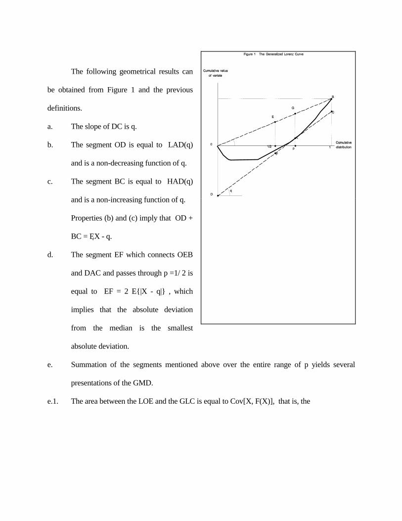
The following geometrical results can

be obtained from Figure 1 and the previous

definitions.

a. The slope of DC is q.

b. The segment OD is equal to LAD(q)

and is a non-decreasing function of q.

c. The segment BC is equal to HAD(q)

and is a non-increasing function of q.

Properties (b) and (c) imply that OD +

BC = EX - q.

d. The segment EF which connects OEB

and DAC and passes through p =1/ 2 is

equal to EF = 2 E{|X - q|} , which

implies that the absolute deviation

from the median is the smallest

absolute deviation.

e. Summation of the segments mentioned above over the entire range of p yields several

presentations of the GMD.

e.1. The area between the LOE and the GLC is equal to Cov[X, F(X)], that is, the

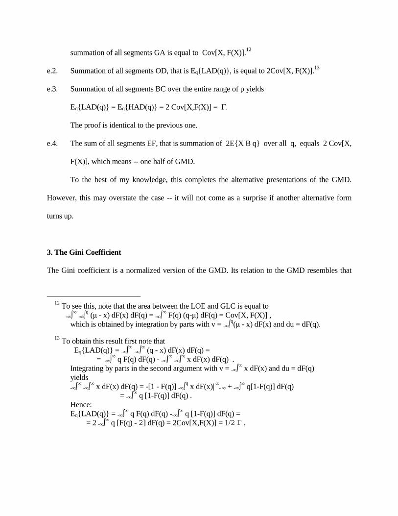
summation of all segments GA is equal to Cov[X, F(X)].12

e.2. Summation of all segments OD, that is Eq{LAD(q)}, is equal to 2Cov[X, F(X)].13

e.3. Summation of all segments BC over the entire range of p yields

Eq{LAD(q)} = Eq{HAD(q)} = 2 Cov[X,F(X)] = Γ.

The proof is identical to the previous one.

e.4. The sum of all segments EF, that is summation of 2E{X B q} over all q, equals 2 Cov[X,

F(X)], which means -- one half of GMD.

To the best of my knowledge, this completes the alternative presentations of the GMD.

However, this may overstate the case -- it will not come as a surprise if another alternative form

turns up.

3. The Gini Coefficient

The Gini coefficient is a normalized version of the GMD. Its relation to the GMD resembles that

12 To see this, note that the area between the LOE and GLC is equal to -∞∫∞ -∞∫q (µ - x) dF(x) dF(q) = -∞∫∞ F(q) (q-µ) dF(q) = Cov[X, F(X)] , which is obtained by integration by parts with v = -∞∫q(µ - x) dF(x) and du = dF(q).

13 To obtain this result first note that Eq{LAD(q)} = -∞∫∞ -∞∫∞ (q - x) dF(x) dF(q) = = -∞∫∞ q F(q) dF(q) - -∞∫∞ -∞∫∞ x dF(x) dF(q) . Integrating by parts in the second argument with v = -∞∫∞ x dF(x) and du = dF(q) yields -∞∫∞ -∞∫∞ x dF(x) dF(q) = -[1 - F(q)] -∞∫q x dF(x)| ∞- ∞ + -∞∫∞ q[1-F(q)] dF(q) = -∞∫∞ q [1-F(q)] dF(q) . Hence: Eq{LAD(q)} = -∞∫∞ q F(q) dF(q) --∞∫∞ q [1-F(q)] dF(q) = = 2 -∞∫∞ q [F(q) - 2] dF(q) = 2Cov[X,F(X)] = 1/2 Γ .

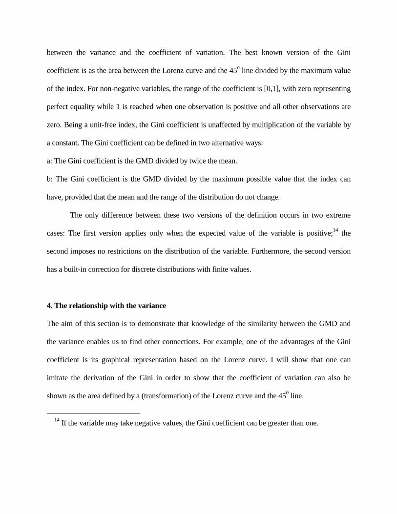
between the variance and the coefficient of variation. The best known version of the Gini

coefficient is as the area between the Lorenz curve and the 45o line divided by the maximum value

of the index. For non-negative variables, the range of the coefficient is [0,1], with zero representing

perfect equality while 1 is reached when one observation is positive and all other observations are

zero. Being a unit-free index, the Gini coefficient is unaffected by multiplication of the variable by

a constant. The Gini coefficient can be defined in two alternative ways:

a: The Gini coefficient is the GMD divided by twice the mean.

b: The Gini coefficient is the GMD divided by the maximum possible value that the index can

have, provided that the mean and the range of the distribution do not change.

The only difference between these two versions of the definition occurs in two extreme

cases: The first version applies only when the expected value of the variable is positive;14 the

second imposes no restrictions on the distribution of the variable. Furthermore, the second version

has a built-in correction for discrete distributions with finite values.

4. The relationship with the variance

The aim of this section is to demonstrate that knowledge of the similarity between the GMD and

the variance enables us to find other connections. For example, one of the advantages of the Gini

coefficient is its graphical representation based on the Lorenz curve. I will show that one can

imitate the derivation of the Gini in order to show that the coefficient of variation can also be

shown as the area defined by a (transformation) of the Lorenz curve and the 450 line.

14 If the variable may take negative values, the Gini coefficient can be greater than one.

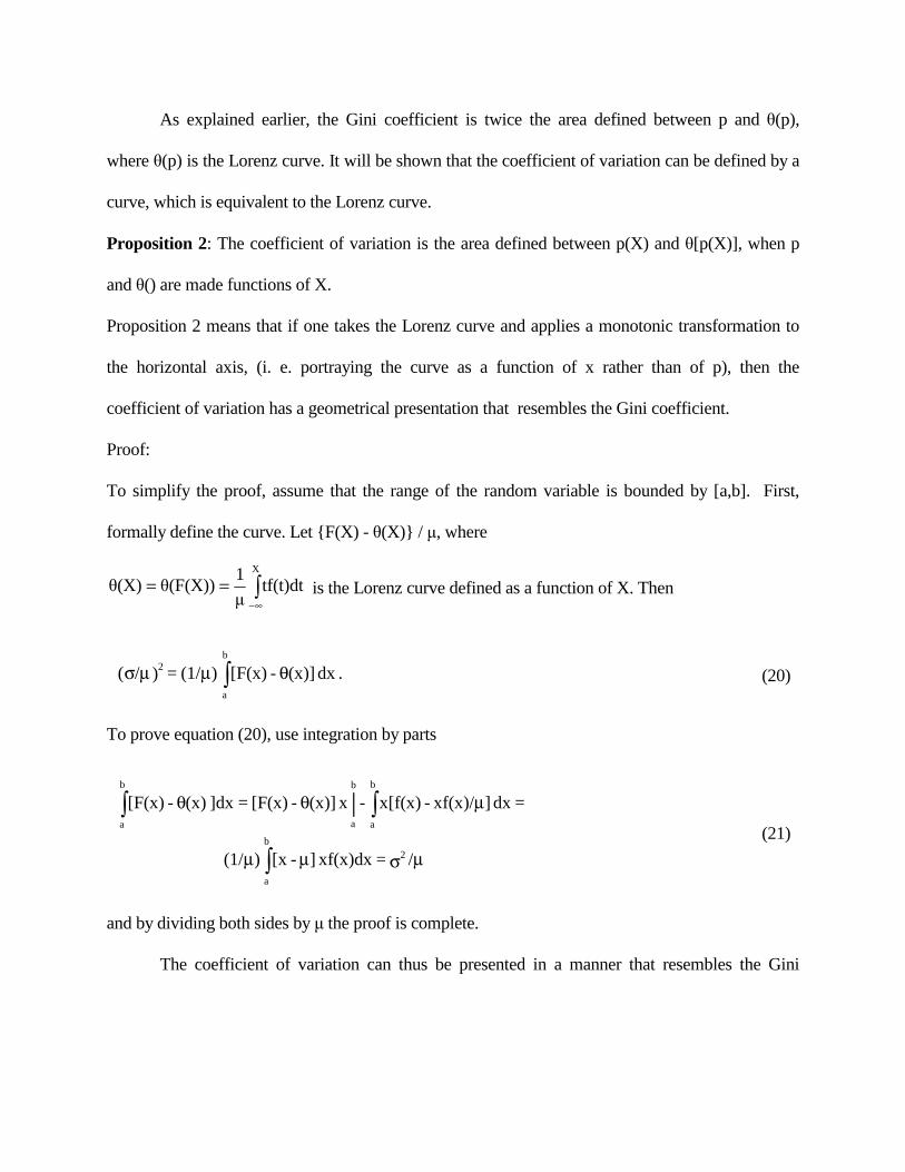
As explained earlier, the Gini coefficient is twice the area defined between p and θ(p),

where θ(p) is the Lorenz curve. It will be shown that the coefficient of variation can be defined by a

curve, which is equivalent to the Lorenz curve.

Proposition 2: The coefficient of variation is the area defined between p(X) and θ[p(X)], when p

and θ() are made functions of X.

Proposition 2 means that if one takes the Lorenz curve and applies a monotonic transformation to

the horizontal axis, (i. e. portraying the curve as a function of x rather than of p), then the

coefficient of variation has a geometrical presentation that resembles the Gini coefficient.

Proof:

To simplify the proof, assume that the range of the random variable is bounded by [a,b]. First,

formally define the curve. Let {F(X) - θ(X)} / µ, where

∫∞−

==X

tf(t)dtµ1θ(F(X))θ(X) is the Lorenz curve defined as a function of X. Then

To prove equation (20), use integration by parts

and by dividing both sides by µ the proof is complete.

The coefficient of variation can thus be presented in a manner that resembles the Gini

.dx (x)] - [F(x) )(1/= )/(b

a

2 θµµσ ∫ (20)

µσµµ

µθθ

∫

∫∫

/ =xf(x)dx ] -[x )(1/

=dx ]xf(x)/ - x[f(x) - x (x)] - [F(x)=]dx (x) - [F(x)

2b

a

b

a

b

a

b

a

| (21)

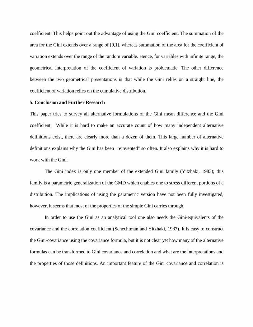
coefficient. This helps point out the advantage of using the Gini coefficient. The summation of the

area for the Gini extends over a range of [0,1], whereas summation of the area for the coefficient of

variation extends over the range of the random variable. Hence, for variables with infinite range, the

geometrical interpretation of the coefficient of variation is problematic. The other difference

between the two geometrical presentations is that while the Gini relies on a straight line, the

coefficient of variation relies on the cumulative distribution.

5. Conclusion and Further Research

This paper tries to survey all alternative formulations of the Gini mean difference and the Gini

coefficient. While it is hard to make an accurate count of how many independent alternative

definitions exist, there are clearly more than a dozen of them. This large number of alternative

definitions explains why the Gini has been "reinvented" so often. It also explains why it is hard to

work with the Gini.

The Gini index is only one member of the extended Gini family (Yitzhaki, 1983); this

family is a parametric generalization of the GMD which enables one to stress different portions of a

distribution. The implications of using the parametric version have not been fully investigated,

however, it seems that most of the properties of the simple Gini carries through.

In order to use the Gini as an analytical tool one also needs the Gini-equivalents of the

covariance and the correlation coefficient (Schechtman and Yitzhaki, 1987). It is easy to construct

the Gini-covariance using the covariance formula, but it is not clear yet how many of the alternative

formulas can be transformed to Gini covariance and correlation and what are the interpretations and

the properties of those definitions. An important feature of the Gini covariance and correlation is

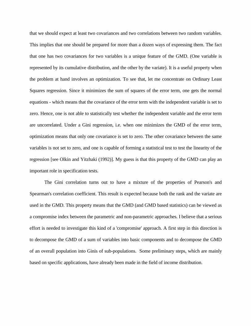
that we should expect at least two covariances and two correlations between two random variables.

This implies that one should be prepared for more than a dozen ways of expressing them. The fact

that one has two covariances for two variables is a unique feature of the GMD. (One variable is

represented by its cumulative distribution, and the other by the variate). It is a useful property when

the problem at hand involves an optimization. To see that, let me concentrate on Ordinary Least

Squares regression. Since it minimizes the sum of squares of the error term, one gets the normal

equations - which means that the covariance of the error term with the independent variable is set to

zero. Hence, one is not able to statistically test whether the independent variable and the error term

are uncorrelated. Under a Gini regression, i.e. when one minimizes the GMD of the error term,

optimization means that only one covariance is set to zero. The other covariance between the same

variables is not set to zero, and one is capable of forming a statistical test to test the linearity of the

regression [see Olkin and Yitzhaki (1992)]. My guess is that this property of the GMD can play an

important role in specification tests.

The Gini correlation turns out to have a mixture of the properties of Pearson's and

Spearman's correlation coefficient. This result is expected because both the rank and the variate are

used in the GMD. This property means that the GMD (and GMD based statistics) can be viewed as

a compromise index between the parametric and non-parametric approaches. I believe that a serious

effort is needed to investigate this kind of a 'compromise' approach. A first step in this direction is

to decompose the GMD of a sum of variables into basic components and to decompose the GMD

of an overall population into Ginis of sub-populations. Some preliminary steps, which are mainly

based on specific applications, have already been made in the field of income distribution.

Finally, The Gini covariances and correlations play an important role in decomposition of

the GMD (Gini coefficient) of a sum of variables (Lerman and Yitzhaki (1985)) and the GMD of

an overall population into the Gini of subgroups. (Yitzhaki (1994). These types of decompositions

are at the early stages of development and beyond the scope of this paper.

References

Bachi, Roberto (1956), "A statistical analysis of the revival of Hebrew in Israel," Scripta

Hierosolymitana III, 179-247.

Bhargava, T. N. and Uppuluri, V. R. R. (1975), "On an axiomatic derivation of Gini diversity, with

applications," Metron, 33, No. 1-2, 41-53.

Buchinsky, Moshe (1991) "Changes in the Structure of Wages in the U. S. 1963-1987:

Application of Quantile and Censored Regressions," Draft. Forthcoming in

Econometrica.

Chandra, Mahesh and Singpurwalla, Nozer, D. (1971), "Relationship between some notions which

are common to reliability theory and economics," Mathematics of Operation Research, 6,

113-121.

Cramer, Harald (1928), "On the composition of elementary errors" (Second paper: Statistical

applications), Skandinavisk Aktuareitidskrift, 11, 141-180.

Dalton, Hugh (1920), "The Measurement of the Inequality of Incomes", The Economic Journal,

(September).

Darling, D. A. (1957), "The Kolmogorov-Smirnov, Cramer-Von Mises Tests," Annals of

Mathematical Statistics, 28, 823-838.

David, H. A. (1968), "Gini's mean difference rediscovered," Biometrika, 55, 573-575.

David, H. A. (1981). Order Statistics (2nd edition), New York: John Wiley & Sons.

Degroot, Morris, H. (1975), Probability and Statistics, London: Addison-Wesley Publishing

Company.

Dennis, B., Patil, G. P., Rossi, O. Stehman, S. and Taille, C. (1979), "A bibliography of literature

on ecological diversity and related methodology." In Ecological Diversity in Theory and

Practice, 1, CPH, 319-354.

Dorfman, Robert (1979), "A formula for the Gini coefficient," Review of Economics and Statistics,

61, (February), 146-149.

Gastwirth, J. L. (1971), "A General Definition of the Lorenz Curve," Econometrica, 39, 1037-1039

Gastwirth, J. L. (1972), The estimation of the Lorenz curve and Gini index. The Review of

Economics and Statistics, 54, 306-316.

Gibbs, Jack, P. and Martin, Walter, A. (1962), "Urbanization, technology and the division of Labor:

international patterns," American Sociological Review, 27 (October), 667-677.

Giorgi, G. M. (1990), "Bibliographic Portrait of the Gini Concentration Ratio," Metron, XLVIII, n

1-4, 183-221.

Giorgi, G. M. (1993), "A Fresh Look at the Topical Interest of the Gini Concentration Ratio,"

Metron, LI, n 1-2, 83-98.

Gini, Corrado (1921), "Measurement of Inequality of Incomes," The Economic Journal, (March),

124-126.

Gini, Corrado (1936) Cowles Commission Research Conference on Economics & Statistics,

Colorado College Publication, General Series No. 208, Colorado Springs.

Hart, P. E. (1975), "Moment distributions in economics: an exposition," Journal of the Royal

Statistical Society, A, 138, Part 3, 423-434.

Harter, H. L. (1978), A Chronological Annotated Bibliography of Order Statistics, Vol 1: Pre-1950,

Washington D. C.: U. S. Government Printing Office.

Hettmansperger, Thomas P. (1984), Statistical Inference based on Ranks, New York: John Wiley

and Sons.

Jaeckel, L. A. (1972), "Estimating regression coefficients by minimizing the dispersion of the

residuals," Annals of Mathematical Statistics, 43, 1449-1458.

Jenkins, S. P. (1988), "Calculating income distribution indices from micro data," National Tax

Journal, 41, 139-142.

Jurečková, J. (1969), "Asymptotic linearity of a rank statistic in regression parameter," Annals of

Mathematical Statistics, 40, 1889-1900.

Koenker, R. and G. Basset, Jr. (1978), "Regression quantiles," Econometrica, 46:33-50.

Lambert, Peter J. (1993), The Distribution and Redistribution of Income, second edition,

Manchester, Manchester University Press.

Lerman, R. and Yitzhaki, S. (1984) "A note on the calculation and interpretation of the Gini index,"

Economics Letters, 15, 353-358.

Lerman, Robert and Yitzhaki, S. “Income Inequality Effects by Income Source: A New Approach

and Application to the U.S.,” Review of Economics and Statistics , 67, No.1, February 1985,

151-56.

Lerman, R. and Yitzhaki, S. (1989), "Improving the accuracy of estimates of Gini coefficients,"

Journal of Econometrics, 42, 43-47.

Lorenz, M. O. (1905), "Methods for measuring concentration of wealth," Journal of American

Statistical Association, 9, New Series No. 70, (June), 209-219.

Lieberson, Stanley, (1969) "Measuring population diversity," American Sociological Review, 34,

(December) 850-862.

Olkin, Ingram and Yitzhaki, S. (1992) "Gini regression analysis," International Statistical Review,

60, 2, (August), 185-196.

Pyatt, Graham, (1976), "On the interpretation and disaggregation of Gini coefficients", The

Economic Journal, 86, (June), 243-255.

Pyatt, Graham, Chau-nan, Chen, and John Fei (1980), "The distribution of income by factor

components," Quarterly Journal of Economics, 95, 451-475.

Rao, C. Radhakrishna, (1982), "Diversity: Its measurement, decomposition, apportionment and

analysis," Sankhya, 44, Series A, Pt. 1, 1-22.

Schechtman, E. and Yitzhaki, S. (1987) "A measure of association based on Gini's mean

difference," Communications in Statistics, A16, No. 1, Theory and Methods, 207-231.

Serfling, Robert, J. (1980), Approximation Theorems of Mathematical Statistics, John Wiley &

Sons, New York.

Shorrocks, A. F. (1983), "Ranking income distributions," Economica, 50, 3-17.

Silber, Jacques (1989), "Facor Components, Populations Subgroups and the Computation of the

Gini Index of Inequality," The Review of Economics and Statistics, 1989, LXXI:107-115.

Simpson, E. H. (1949), "Measurement of diversity," Nature, 163, 688.

Smirnov, N. V. (1937), "On the Distribution of the w2 criterion of von Mises," Rec. Math. (NS) 2,

973-993.

Stuart, Alan (1954), The Correlation between variate-values and ranks in samples from a

continuous distributions," British Journal of Statistical Psychology 7, 37-44

von Mises, R. (1931), Wahrscheinlichkeitsrechnung, Leipzig-Wien

Wold, Herman (1935), "A study of the mean difference, concentration curves and concentration

ratios," Metron, 12, No. 2, 39-58.

Yaari, M. E. (1988) "A controversial proposal concerning inequality measurement," Journal of

Economic Theory, 44, No. 2, 381-97.

Yitzhaki, S. (1983), "On an extension of the Gini inequality index," International Economic

Review, 24, No. 3, (October), 617-28.

Yitzhaki, S. (1994), “Economic Distance and Overlapping of Distributions,” Journal of

Econometrics , Vol 61, 147-159.