Morphological filters for OCR: a performance comparison

Laurent Mennillo1, Jean Cousty2 and Laurent Najman2

1Institut Pascal - UMR6602 - UBP/CNRS/IFMA2Universite Paris-Est, LIGM, Equipe A3SI, ESIEE, France

AbstractIn this article is compared the ability of several morphological operators to improve OCR

performance when used as preprocessing filters. An experiment on binary and greyscaleimages using the Tesseract OCR engine and morphological filters acting in complex, graphand vertex spaces has thus been performed and results in a good overall performance ofcomplex and area filters. MSE measures have also been performed to evaluate the denoisingability of these filters, which again shows the good performance of both complex and areafilters on this aspect.

1 Introduction

This article presents an OCR performance comparison obtained through the use of several mor-phological filters on degraded documents. First, section 2 will present the degradation modelsused to alter the documents to be analysed, section 3 will then introduce morphological filterspartially restoring the image quality of such degraded documents, section 4 will describe thedetailed test protocols of this experiment and the last sections will finally discuss the results andconclude.

2 Document degradation models

Document degradation models are designed to simulate local distortions that are introducedduring the processes of document scanning, printing and photocopying. In the context of thisexperiment, some of these models have the ability to generate realistic degradations that areappropriate for OCR performance evaluation. Besides, increasing levels of such degradations canalso be produced by adjusting the models parameters, thus allowing a proper leveled comparison.

2.1 Binary document degradation

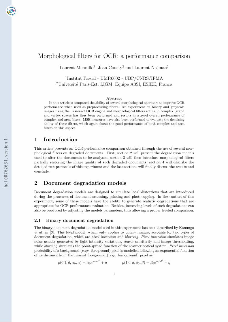
The binary document degradation model used in this experiment has been described by Kanungoet al. in [3]. This local model, which only applies to binary images, accounts for two types ofdocument degradation, which are pixel inversion and blurring. Pixel inversion simulates imagenoise usually generated by light intensity variations, sensor sensitivity and image thresholding,while blurring simulates the point-spread function of the scanner optical system. Pixel inversionprobability of a background (resp. foreground) pixel is modelled following an exponential functionof its distance from the nearest foreground (resp. background) pixel as:

p(0|1, d, α0, α) = α0e−αd2 + η p(1|0, d, β0, β) = β0e

−βd2 + η

1

hal-0

0762

631,

ver

sion

1 -

Parameter d is thus the 4-neighbor distance of each background (resp. foreground) pixel fromits nearest foreground (resp. background) pixel, parameter α0 (resp. β0) is the amount ofgenerated noise related to background (resp. foreground) pixels, parameter α (resp. β) is thedecay speed, relatively to distance d, of background (resp. foreground) pixels flipping probabilityand parameter η is the constant flipping probability of all pixels. Finally, Blurring is produced bya morphological closing operation using a disk structuring element of diameter k. The describedmodel with parameters Θ = (η, α0, α, β0, β, k) is thus used to degrade any binary document bycomputing the distance map of each pixel, then independently flip them following their respectiveprobability and finally perform a morphological closing operation.

2.2 Greyscale document degradation

The document degradation model described in 2.1 can also be used to process greyscale images.For this purpose, the image to degrade is first thresholded with value t ∈ [0; 255] to binary imagesBt. These images are then degraded with the binary document degradation model. Thereafter,greyscale images Gt are generated by setting the black pixels of images Bt to their respectivetresholding value t. The degraded image D, initialized with white pixels, is finally reconstructedfrom white to black values (t = 255 . . . 0) by processing the minimum value at each pixelof images D and Gt (Di,j = min(Di,j , Gt,i,j)). In this experiment, a faster but less realisticgreyscale document degradation is achieved by adding impulsional Gaussian noise to the originalimage with parameters Ω = (σ, p), where σ and p, respectively denote the standard deviationand proportion of pixels to alter.

3 Morphological filtering

Morphological filters can be used to restore or improve the image quality of digitally converteddocuments and thus increase OCR performance. This section presents the four morphologicalfilters compared in this experiment.

3.1 Morphological operators in simplicial complex spaces

Morphological operators defined in simplicial complex spaces have been presented by Dias et al.in [2]. The following paragraphs will introduce these morphological operators and describe theirimplementation.

3.1.1 Definitions

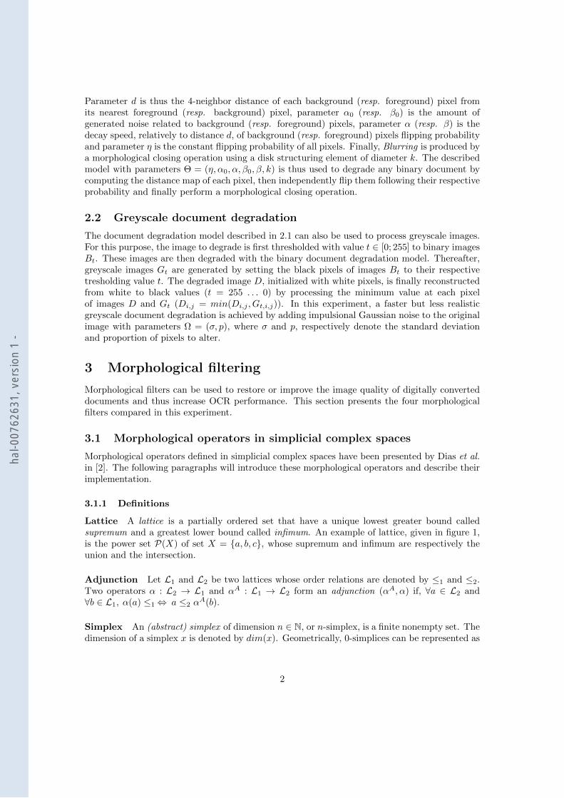
Lattice A lattice is a partially ordered set that have a unique lowest greater bound calledsupremum and a greatest lower bound called infimum. An example of lattice, given in figure 1,is the power set P(X) of set X = a, b, c, whose supremum and infimum are respectively theunion and the intersection.

Adjunction Let L1 and L2 be two lattices whose order relations are denoted by ≤1 and ≤2.Two operators α : L2 → L1 and αA : L1 → L2 form an adjunction (αA, α) if, ∀a ∈ L2 and∀b ∈ L1, α(a) ≤1⇔ a ≤2 α

A(b).

Simplex An (abstract) simplex of dimension n ∈ N, or n-simplex, is a finite nonempty set. Thedimension of a simplex x is denoted by dim(x). Geometrically, 0-simplices can be represented as

2

hal-0

0762

631,

ver

sion

1 -

a,b,c

b,ca,ca,b

b ca

Ø

Figure 1: Power set P(X) of set X = a, b, c.

points, 1-simplices as segments, 2-simplices as triangles and so forth. Illustrations of simplicesa, a, b and a, b, c are respectively given in figures 2a, 2b and 2c.

a

(a) 0-simplex

a b

(b) 1-simplex

a b

c

(c) 2-simplex

a b

c

(d) 2-cell

Figure 2: Graphical representation of simplices and cell.

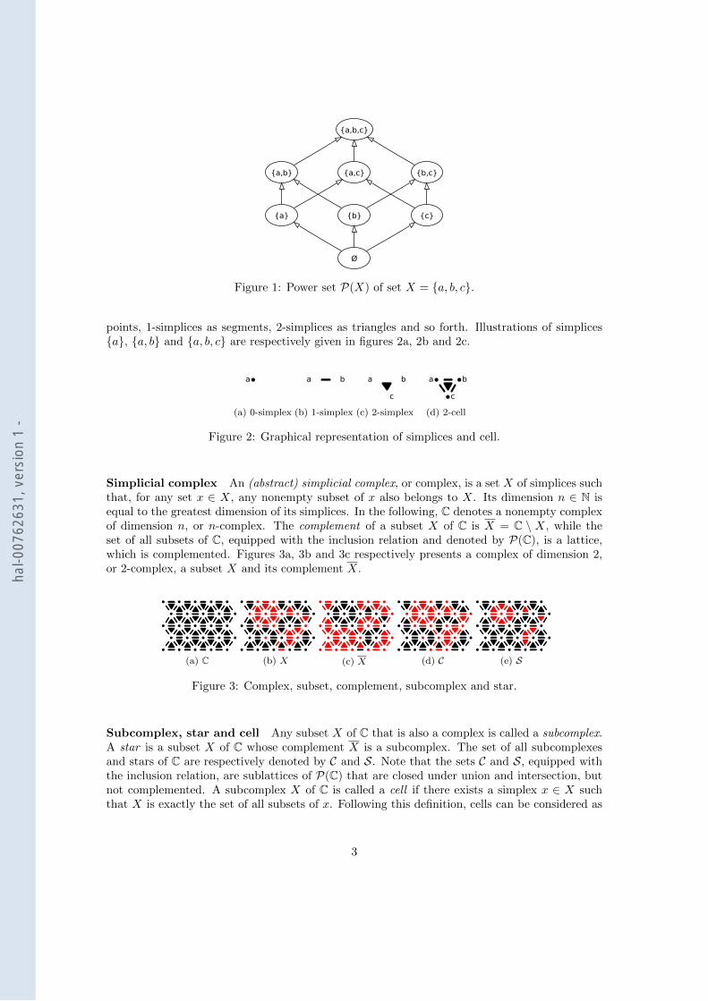
Simplicial complex An (abstract) simplicial complex, or complex, is a set X of simplices suchthat, for any set x ∈ X, any nonempty subset of x also belongs to X. Its dimension n ∈ N isequal to the greatest dimension of its simplices. In the following, C denotes a nonempty complexof dimension n, or n-complex. The complement of a subset X of C is X = C \ X, while theset of all subsets of C, equipped with the inclusion relation and denoted by P(C), is a lattice,which is complemented. Figures 3a, 3b and 3c respectively presents a complex of dimension 2,or 2-complex, a subset X and its complement X.

(a) C (b) X (c) X (d) C (e) S

Figure 3: Complex, subset, complement, subcomplex and star.

Subcomplex, star and cell Any subset X of C that is also a complex is called a subcomplex.A star is a subset X of C whose complement X is a subcomplex. The set of all subcomplexesand stars of C are respectively denoted by C and S. Note that the sets C and S, equipped withthe inclusion relation, are sublattices of P(C) that are closed under union and intersection, butnot complemented. A subcomplex X of C is called a cell if there exists a simplex x ∈ X suchthat X is exactly the set of all subsets of x. Following this definition, cells can be considered as

3

hal-0

0762

631,

ver

sion

1 -

the elementary building blocks of simplicial complexes. Illustrations of a subcomplex, a star anda cell are respectively given in figures 3d, 3e and 2d.

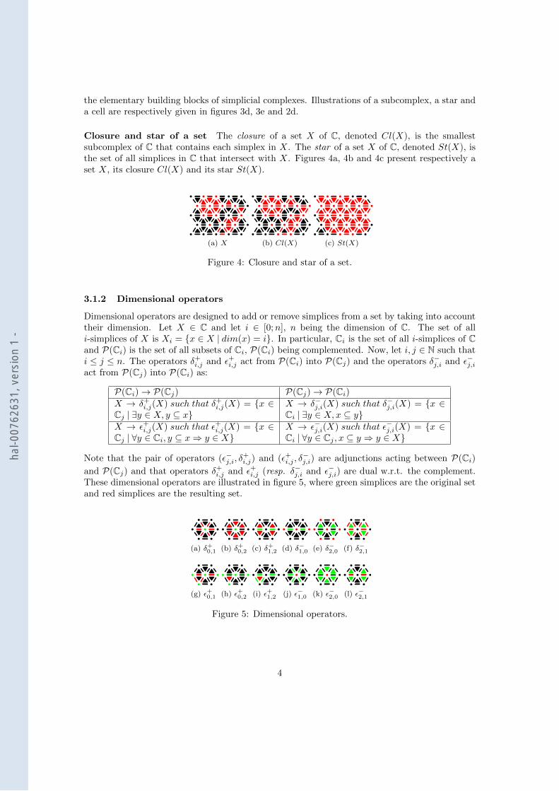
Closure and star of a set The closure of a set X of C, denoted Cl(X), is the smallestsubcomplex of C that contains each simplex in X. The star of a set X of C, denoted St(X), isthe set of all simplices in C that intersect with X. Figures 4a, 4b and 4c present respectively aset X, its closure Cl(X) and its star St(X).

(a) X (b) Cl(X) (c) St(X)

Figure 4: Closure and star of a set.

3.1.2 Dimensional operators

Dimensional operators are designed to add or remove simplices from a set by taking into accounttheir dimension. Let X ∈ C and let i ∈ [0;n], n being the dimension of C. The set of alli-simplices of X is Xi = x ∈ X | dim(x) = i. In particular, Ci is the set of all i-simplices of Cand P(Ci) is the set of all subsets of Ci, P(Ci) being complemented. Now, let i, j ∈ N such thati ≤ j ≤ n. The operators δ+i,j and ε+i,j act from P(Ci) into P(Cj) and the operators δ−j,i and ε−j,iact from P(Cj) into P(Ci) as:

P(Ci)→ P(Cj) P(Cj)→ P(Ci)X → δ+i,j(X) such that δ+i,j(X) = x ∈Cj | ∃y ∈ X, y ⊆ x

X → δ−j,i(X) such that δ−j,i(X) = x ∈Ci | ∃y ∈ X,x ⊆ y

X → ε+i,j(X) such that ε+i,j(X) = x ∈Cj | ∀y ∈ Ci, y ⊆ x⇒ y ∈ X

X → ε−j,i(X) such that ε−j,i(X) = x ∈Ci | ∀y ∈ Cj , x ⊆ y ⇒ y ∈ X

Note that the pair of operators (ε−j,i, δ+i,j) and (ε+i,j , δ

−j,i) are adjunctions acting between P(Ci)

and P(Cj) and that operators δ+i,j and ε+i,j (resp. δ−j,i and ε−j,i) are dual w.r.t. the complement.These dimensional operators are illustrated in figure 5, where green simplices are the original setand red simplices are the resulting set.

(a) δ+0,1 (b) δ+0,2 (c) δ+1,2 (d) δ−1,0 (e) δ−2,0 (f) δ−2,1

(g) ε+0,1 (h) ε+0,2 (i) ε+1,2 (j) ε−1,0 (k) ε−2,0 (l) ε−2,1

Figure 5: Dimensional operators.

4

hal-0

0762

631,

ver

sion

1 -

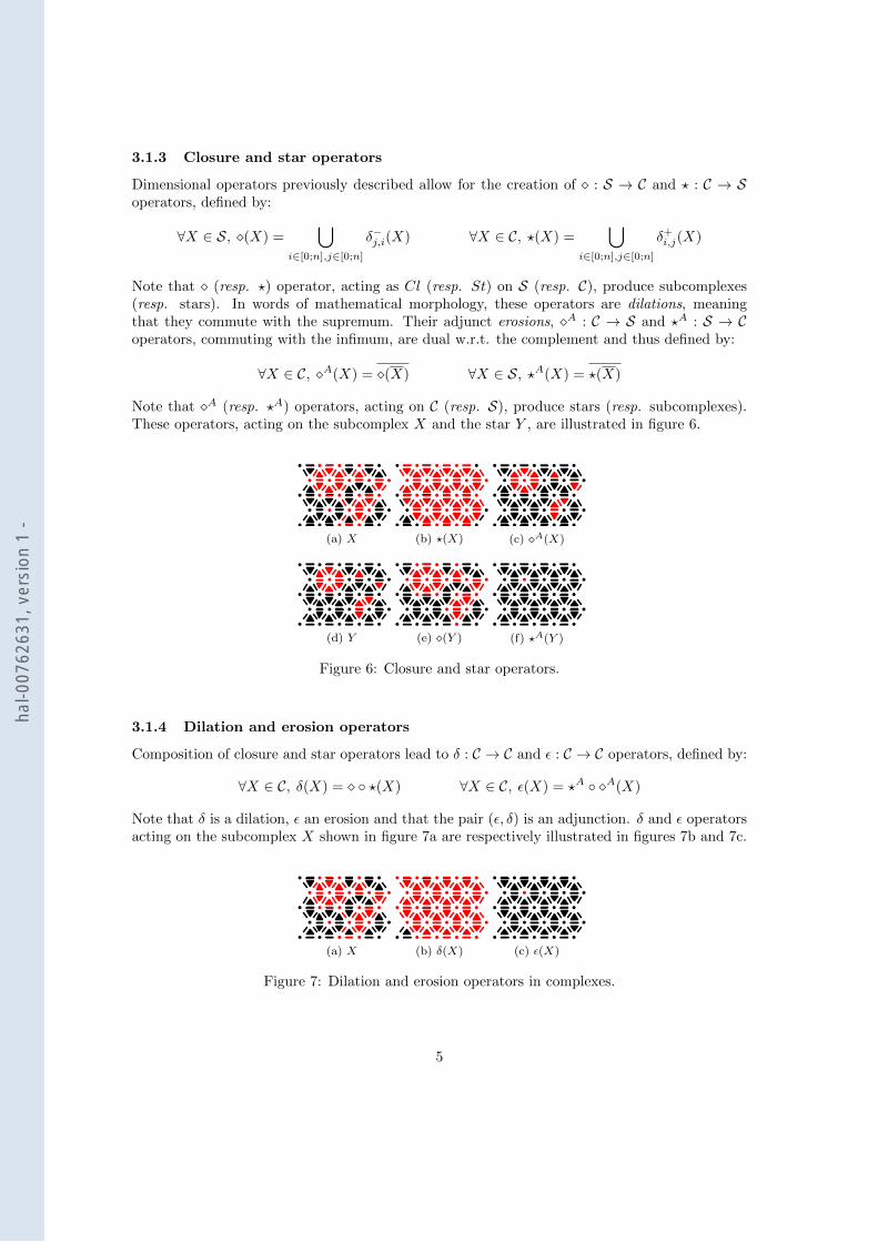
3.1.3 Closure and star operators

Dimensional operators previously described allow for the creation of : S → C and ? : C → Soperators, defined by:

∀X ∈ S, (X) =⋃

i∈[0;n],j∈[0;n]

δ−j,i(X) ∀X ∈ C, ?(X) =⋃

i∈[0;n],j∈[0;n]

δ+i,j(X)

Note that (resp. ?) operator, acting as Cl (resp. St) on S (resp. C), produce subcomplexes(resp. stars). In words of mathematical morphology, these operators are dilations, meaningthat they commute with the supremum. Their adjunct erosions, A : C → S and ?A : S → Coperators, commuting with the infimum, are dual w.r.t. the complement and thus defined by:

∀X ∈ C, A(X) = (X) ∀X ∈ S, ?A(X) = ?(X)

Note that A (resp. ?A) operators, acting on C (resp. S), produce stars (resp. subcomplexes).These operators, acting on the subcomplex X and the star Y , are illustrated in figure 6.

(a) X (b) ?(X) (c) A(X)

(d) Y (e) (Y ) (f) ?A(Y )

Figure 6: Closure and star operators.

3.1.4 Dilation and erosion operators

Composition of closure and star operators lead to δ : C → C and ε : C → C operators, defined by:

∀X ∈ C, δ(X) = ?(X) ∀X ∈ C, ε(X) = ?A A(X)

Note that δ is a dilation, ε an erosion and that the pair (ε, δ) is an adjunction. δ and ε operatorsacting on the subcomplex X shown in figure 7a are respectively illustrated in figures 7b and 7c.

(a) X (b) δ(X) (c) ε(X)

Figure 7: Dilation and erosion operators in complexes.

5

hal-0

0762

631,

ver

sion

1 -

3.1.5 Closing and opening filters

A filter is an operator β : L → L that is increasing: X ⊆ Y ⇒ β(X) ⊆ β(Y ) and idempotent:β β(X) = β(X). Composition of dilation and erosion operators lead to φ : C → C and γ : C → Cfilters, defined by:

∀X ∈ C, φ(X) = ε δ(X) ∀X ∈ C, γ(X) = δ ε(X)

In words of mathematical morphology, φ filter is a closing operation, which is extensive: X ⊆φ(X), while γ filter is an opening operation, which is anti-extensive: γ(X) ⊆ X. These twofilters are illustrated in figure 8.

(a) X (b) φ(X) (c) γ(X)

Figure 8: Closing and opening filters in complexes.

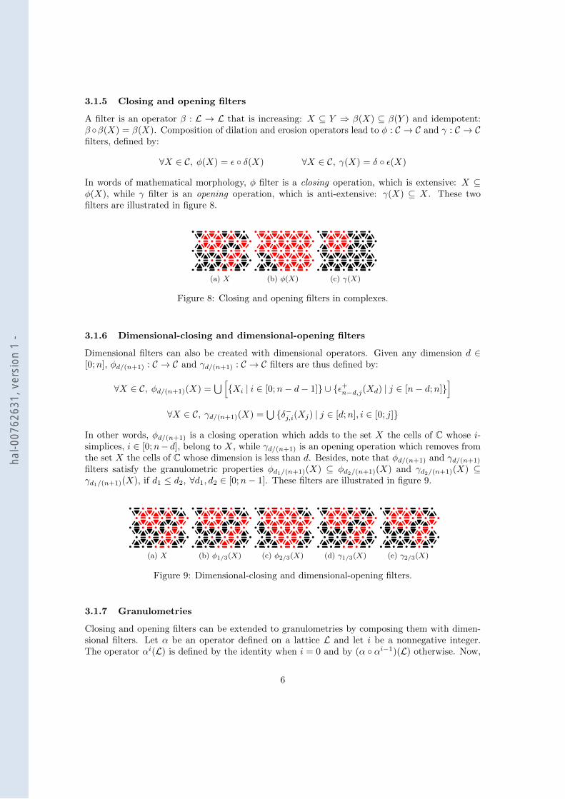
3.1.6 Dimensional-closing and dimensional-opening filters

Dimensional filters can also be created with dimensional operators. Given any dimension d ∈[0;n], φd/(n+1) : C → C and γd/(n+1) : C → C filters are thus defined by:

∀X ∈ C, φd/(n+1)(X) =⋃[Xi | i ∈ [0;n− d− 1] ∪ ε+n−d,j(Xd) | j ∈ [n− d;n]

]∀X ∈ C, γd/(n+1)(X) =

⋃δ−j,i(Xj) | j ∈ [d;n], i ∈ [0; j]

In other words, φd/(n+1) is a closing operation which adds to the set X the cells of C whose i-simplices, i ∈ [0;n− d], belong to X, while γd/(n+1) is an opening operation which removes fromthe set X the cells of C whose dimension is less than d. Besides, note that φd/(n+1) and γd/(n+1)

filters satisfy the granulometric properties φd1/(n+1)(X) ⊆ φd2/(n+1)(X) and γd2/(n+1)(X) ⊆γd1/(n+1)(X), if d1 ≤ d2, ∀d1, d2 ∈ [0;n− 1]. These filters are illustrated in figure 9.

(a) X (b) φ1/3(X) (c) φ2/3(X) (d) γ1/3(X) (e) γ2/3(X)

Figure 9: Dimensional-closing and dimensional-opening filters.

3.1.7 Granulometries

Closing and opening filters can be extended to granulometries by composing them with dimen-sional filters. Let α be an operator defined on a lattice L and let i be a nonnegative integer.The operator αi(L) is defined by the identity when i = 0 and by (α αi−1)(L) otherwise. Now,

6

hal-0

0762

631,

ver

sion

1 -

let parameters i and d respectively be the quotient and the remainder of the division k/(n+ 1).Granulometric-closing filter Φk/(n+1) : C → C and granulometric-opening filter Γk/(n+1) : C → Care then defined by:

∀X ∈ C, Φk/(n+1) = εi φd/(n+1) δi(X) ∀X ∈ C, Γk/(n+1) = δi γd/(n+1) εi(X)

3.1.8 Alternating sequential filter

The alternating sequential filter ASFk/(n+1) : C → C can be defined using the granulometricclosing and opening filters by:

∀X ∈ C, ASFk/(n+1)(X) =

identity if k = 0Γk/(n+1) Φk/(n+1) ASFk−1/(n+1)(X) otherwise

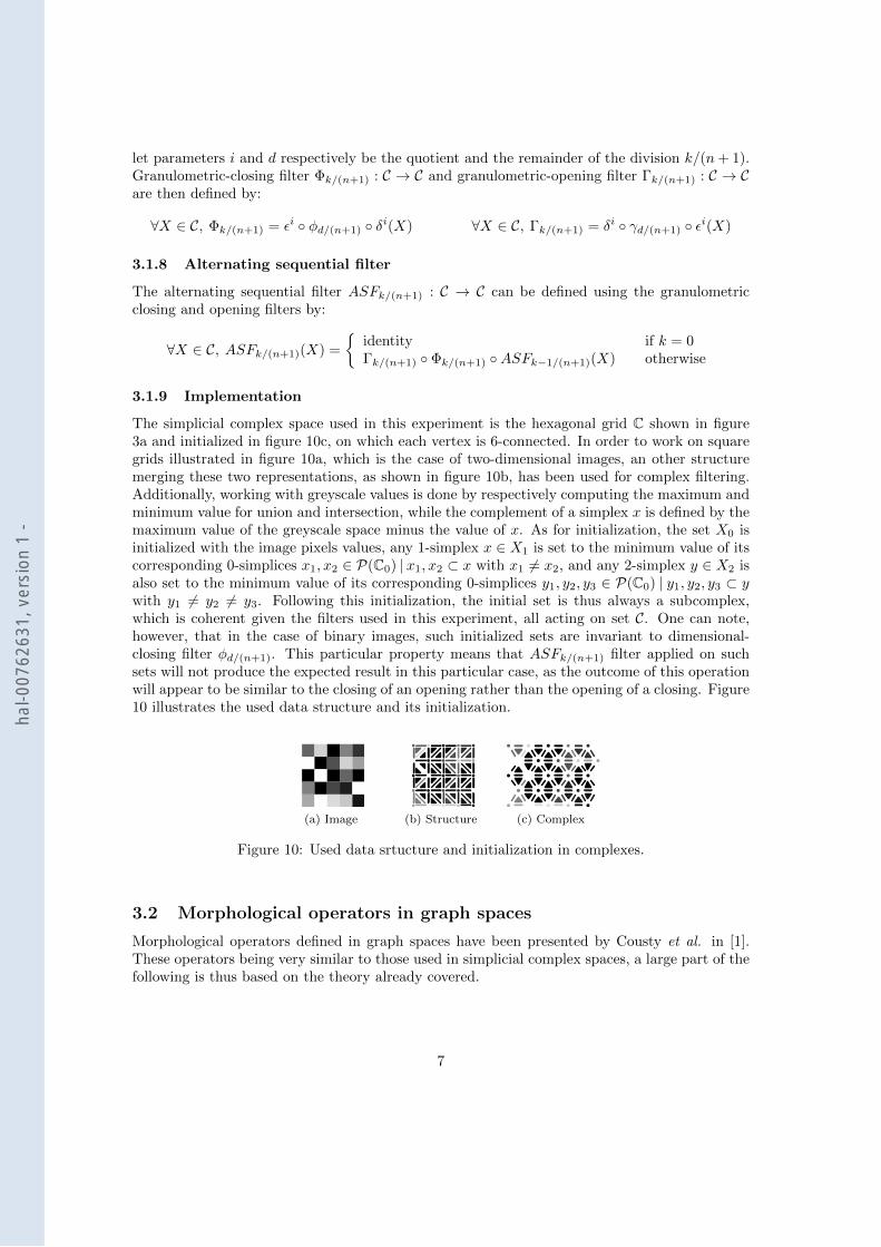
3.1.9 Implementation

The simplicial complex space used in this experiment is the hexagonal grid C shown in figure3a and initialized in figure 10c, on which each vertex is 6-connected. In order to work on squaregrids illustrated in figure 10a, which is the case of two-dimensional images, an other structuremerging these two representations, as shown in figure 10b, has been used for complex filtering.Additionally, working with greyscale values is done by respectively computing the maximum andminimum value for union and intersection, while the complement of a simplex x is defined by themaximum value of the greyscale space minus the value of x. As for initialization, the set X0 isinitialized with the image pixels values, any 1-simplex x ∈ X1 is set to the minimum value of itscorresponding 0-simplices x1, x2 ∈ P(C0) | x1, x2 ⊂ x with x1 6= x2, and any 2-simplex y ∈ X2 isalso set to the minimum value of its corresponding 0-simplices y1, y2, y3 ∈ P(C0) | y1, y2, y3 ⊂ ywith y1 6= y2 6= y3. Following this initialization, the initial set is thus always a subcomplex,which is coherent given the filters used in this experiment, all acting on set C. One can note,however, that in the case of binary images, such initialized sets are invariant to dimensional-closing filter φd/(n+1). This particular property means that ASFk/(n+1) filter applied on suchsets will not produce the expected result in this particular case, as the outcome of this operationwill appear to be similar to the closing of an opening rather than the opening of a closing. Figure10 illustrates the used data structure and its initialization.

(a) Image (b) Structure (c) Complex

Figure 10: Used data srtucture and initialization in complexes.

3.2 Morphological operators in graph spaces

Morphological operators defined in graph spaces have been presented by Cousty et al. in [1].These operators being very similar to those used in simplicial complex spaces, a large part of thefollowing is thus based on the theory already covered.

7

hal-0

0762

631,

ver

sion

1 -

3.2.1 Definitions

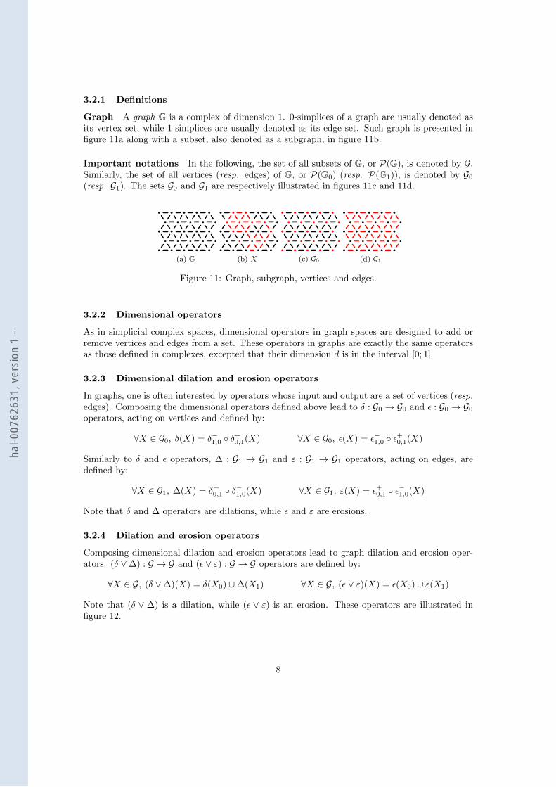
Graph A graph G is a complex of dimension 1. 0-simplices of a graph are usually denoted asits vertex set, while 1-simplices are usually denoted as its edge set. Such graph is presented infigure 11a along with a subset, also denoted as a subgraph, in figure 11b.

Important notations In the following, the set of all subsets of G, or P(G), is denoted by G.Similarly, the set of all vertices (resp. edges) of G, or P(G0) (resp. P(G1)), is denoted by G0(resp. G1). The sets G0 and G1 are respectively illustrated in figures 11c and 11d.

(a) G (b) X (c) G0 (d) G1

Figure 11: Graph, subgraph, vertices and edges.

3.2.2 Dimensional operators

As in simplicial complex spaces, dimensional operators in graph spaces are designed to add orremove vertices and edges from a set. These operators in graphs are exactly the same operatorsas those defined in complexes, excepted that their dimension d is in the interval [0; 1].

3.2.3 Dimensional dilation and erosion operators

In graphs, one is often interested by operators whose input and output are a set of vertices (resp.edges). Composing the dimensional operators defined above lead to δ : G0 → G0 and ε : G0 → G0operators, acting on vertices and defined by:

∀X ∈ G0, δ(X) = δ−1,0 δ+0,1(X) ∀X ∈ G0, ε(X) = ε−1,0 ε

+0,1(X)

Similarly to δ and ε operators, ∆ : G1 → G1 and ε : G1 → G1 operators, acting on edges, aredefined by:

∀X ∈ G1, ∆(X) = δ+0,1 δ−1,0(X) ∀X ∈ G1, ε(X) = ε+0,1 ε

−1,0(X)

Note that δ and ∆ operators are dilations, while ε and ε are erosions.

3.2.4 Dilation and erosion operators

Composing dimensional dilation and erosion operators lead to graph dilation and erosion oper-ators. (δ ∨∆) : G → G and (ε ∨ ε) : G → G operators are defined by:

∀X ∈ G, (δ ∨∆)(X) = δ(X0) ∪∆(X1) ∀X ∈ G, (ε ∨ ε)(X) = ε(X0) ∪ ε(X1)

Note that (δ ∨ ∆) is a dilation, while (ε ∨ ε) is an erosion. These operators are illustrated infigure 12.

8

hal-0

0762

631,

ver

sion

1 -

(a) X (b) (δ ∨∆)(X) (c) (ε ∨ ε)(X)

Figure 12: Graph dilation and erosion operators.

3.2.5 Closing and opening filters

Composition of δ, ∆, ε and ε operators lead to (φ ∨ Φ)1 : G → G and (γ ∨ Γ)1 : G → G filters,defined by:

∀X ∈ G, (φ ∨ Φ)1(X) = (ε ∨ ε) (δ ∨∆)(X)

∀X ∈ G, (γ ∨ Γ)1(X) = (δ ∨∆) (ε ∨ ε)(X)

Note that (φ ∨ Φ)1 is a closing operation, while (γ ∨ Γ)1 is an opening operation. These filtersare illustrated in figure 13.

(a) X (b) (φ ∨ Φ)1(X) (c) (γ ∨ Γ)1(X)

Figure 13: Graph closing and opening filters.

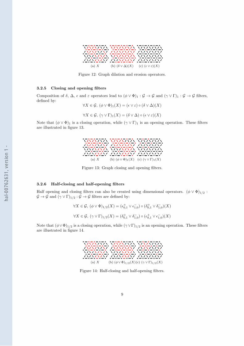
3.2.6 Half-closing and half-opening filters

Half opening and closing filters can also be created using dimensional operators. (φ ∨ Φ)1/2 :G → G and (γ ∨ Γ)1/2 : G → G filters are defined by:

∀X ∈ G, (φ ∨ Φ)1/2(X) = (ε+0,1 ∨ ε−1,0) (δ+0,1 ∨ δ

−1,0)(X)

∀X ∈ G, (γ ∨ Γ)1/2(X) = (δ+0,1 ∨ δ−1,0) (ε+0,1 ∨ ε

−1,0)(X)

Note that (φ∨Φ)1/2 is a closing operation, while (γ∨Γ)1/2 is an opening operation. These filtersare illustrated in figure 14.

(a) X (b) (φ∨Φ)1/2(X)(c) (γ ∨ Γ)1/2(X)

Figure 14: Half-closing and half-opening filters.

9

hal-0

0762

631,

ver

sion

1 -

3.2.7 Granulometries

Given parameters i and j, respectively being the quotient and the remainder of the division k/2,granulometric-closing filter (φ∨Φ)k/2 : G → G and granulometric-opening filter (γ∨Γ)k/2 : G → Gare defined by:

∀X ∈ G, (φ ∨ Φ)k/2 = (ε ∨ ε)i (φ ∨ Φ)j1/2 (δ ∨∆)i(X)

∀X ∈ G, (γ ∨ Γ)k/2 = (δ ∨∆)i (γ ∨ Γ)j1/2 (ε ∨ ε)i(X)

3.2.8 Alternating sequential filter

The alternating sequential filter ASFk/2 : G → G can be defined using the granulometries definedabove, by:

∀X ∈ G, ASFk/2(X) =

identity if k = 0(γ ∨ Γ)k/2 (φ ∨ Φ)k/2 ASFk−1/2(X) otherwise

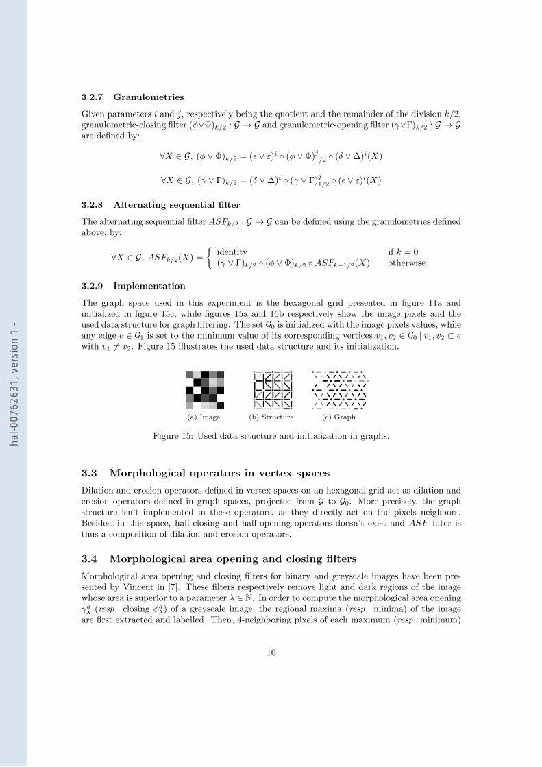
3.2.9 Implementation

The graph space used in this experiment is the hexagonal grid presented in figure 11a andinitialized in figure 15c, while figures 15a and 15b respectively show the image pixels and theused data structure for graph filtering. The set G0 is initialized with the image pixels values, whileany edge e ∈ G1 is set to the minimum value of its corresponding vertices v1, v2 ∈ G0 | v1, v2 ⊂ ewith v1 6= v2. Figure 15 illustrates the used data structure and its initialization.

(a) Image (b) Structure (c) Graph

Figure 15: Used data srtucture and initialization in graphs.

3.3 Morphological operators in vertex spaces

Dilation and erosion operators defined in vertex spaces on an hexagonal grid act as dilation anderosion operators defined in graph spaces, projected from G to G0. More precisely, the graphstructure isn’t implemented in these operators, as they directly act on the pixels neighbors.Besides, in this space, half-closing and half-opening operators doesn’t exist and ASF filter isthus a composition of dilation and erosion operators.

3.4 Morphological area opening and closing filters

Morphological area opening and closing filters for binary and greyscale images have been pre-sented by Vincent in [7]. These filters respectively remove light and dark regions of the imagewhose area is superior to a parameter λ ∈ N. In order to compute the morphological area openingγaλ (resp. closing φaλ) of a greyscale image, the regional maxima (resp. minima) of the imageare first extracted and labelled. Then, 4-neighboring pixels of each maximum (resp. minimum)

10

hal-0

0762

631,

ver

sion

1 -

are progressively added relatively to their intensity, from light (resp. dark) to dark (resp. light)pixels, until the area of the broadened regions reaches λ. Pixels of the created regions are finallyset to the intensity value of their last added pixel.

4 Test protocols

4.1 First test protocol

Tesseract OCR engine, presented in [6], has been used to perform optical character recognitionin this experiment. This powerful system has been evaluated by UNLV-ISRI in 1995 (referto [4]) along with other commercial OCR engines and proved its top-tier performance at thetime. In order to get OCR performance results from this engine on preprocessed documents,the test data and software tools from UNLV-ISRI presented in [5] have been used. Most of thedocuments in this test data being available in binary format at 300 DPI resolution, the testshave been conducted on a selection of this particular set of documents (100). An other set oftwo generated greyscale documents has been used to evaluate the performance of each filter ongreyscale values. The test procedure is basically the iteration of degradation, filtering, OCRanalysis and MSE measure of each document, repeated for each couple (d, f) of degradation andfiltering parameters. Note, however, that the used binary documents are scanned versions ofreal documents, meaning that they are imperfect and consequently contain noise. Degradationperformed on these documents simply allow for a better comparison of the filters efficiency incritical conditions.

4.1.1 Degradation

Degradation levels are specified with parameter d ∈ N, which acts on the binary document degra-dation model parameters Θ = (η, α0, α, β0, β, k) and the impulsional Gaussian noise parametersΩ = (σ, p) as follows:

Θ(d) = (d ∗ 0.02, d ∗ 0.1, 1, d ∗ 0.1, 1, 0)

Ω(d) = (128, d ∗ 0.1)

4.1.2 Filtering

The filters used in this experiment are the ASF filters in simplicial complexes, graphs and ver-tices, as well as a combination of area closing and area opening filters. The tests have beenconducted on both regular and inverse versions of each document, in particular to evaluate theimpact of the proposed initialization in simplicial complex spaces on binary documents. Fur-thermore, ASF filters in gaphs and vertices have also been evaluated with document resolutionscaling of respectively 3/1 and 3/2 (Usc), in order to preserve the same number of iterationsbetween each filter. In the case of binary document filtering, the corresponding upscaled docu-ments were then binarized with a threshold value of 128 (Thr1), downscaled to their original sizeafter filtering (Dsc) and binarized again with a threshold value of 128 (Thr2) in order to pre-serve the characters size for OCR processing. As for greyscale documents, they were also scaledbut not thresholded. Filtering levels were specified for each morphological filter with parameterf ∈ N. Detailed settings are described in table 1. One can note that binarization after upscaling(Thr1) is not performed in the case of vertices filtering. This is simply due to the fact that thesedocuments are already in binary form after an exact upscaling of 3/1.

11

hal-0

0762

631,

ver

sion

1 -

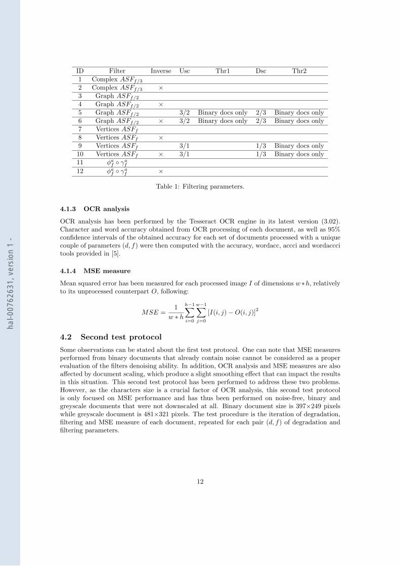
ID Filter Inverse Usc Thr1 Dsc Thr21 Complex ASFf/32 Complex ASFf/3 ×3 Graph ASFf/24 Graph ASFf/2 ×5 Graph ASFf/2 3/2 Binary docs only 2/3 Binary docs only6 Graph ASFf/2 × 3/2 Binary docs only 2/3 Binary docs only7 Vertices ASFf8 Vertices ASFf ×9 Vertices ASFf 3/1 1/3 Binary docs only10 Vertices ASFf × 3/1 1/3 Binary docs only11 φaf γaf12 φaf γaf ×

Table 1: Filtering parameters.

4.1.3 OCR analysis

OCR analysis has been performed by the Tesseract OCR engine in its latest version (3.02).Character and word accuracy obtained from OCR processing of each document, as well as 95%confidence intervals of the obtained accuracy for each set of documents processed with a uniquecouple of parameters (d, f) were then computed with the accuracy, wordacc, accci and wordacccitools provided in [5].

4.1.4 MSE measure

Mean squared error has been measured for each processed image I of dimensions w ∗h, relativelyto its unprocessed counterpart O, following:

MSE =1

w ∗ h

h−1∑i=0

w−1∑j=0

[I(i, j)−O(i, j)]2

4.2 Second test protocol

Some observations can be stated about the first test protocol. One can note that MSE measuresperformed from binary documents that already contain noise cannot be considered as a properevaluation of the filters denoising ability. In addition, OCR analysis and MSE measures are alsoaffected by document scaling, which produce a slight smoothing effect that can impact the resultsin this situation. This second test protocol has been performed to address these two problems.However, as the characters size is a crucial factor of OCR analysis, this second test protocolis only focused on MSE performance and has thus been performed on noise-free, binary andgreyscale documents that were not downscaled at all. Binary document size is 397×249 pixelswhile greyscale document is 481×321 pixels. The test procedure is the iteration of degradation,filtering and MSE measure of each document, repeated for each pair (d, f) of degradation andfiltering parameters.

12

hal-0

0762

631,

ver

sion

1 -

5 Results

5.1 First test protocol

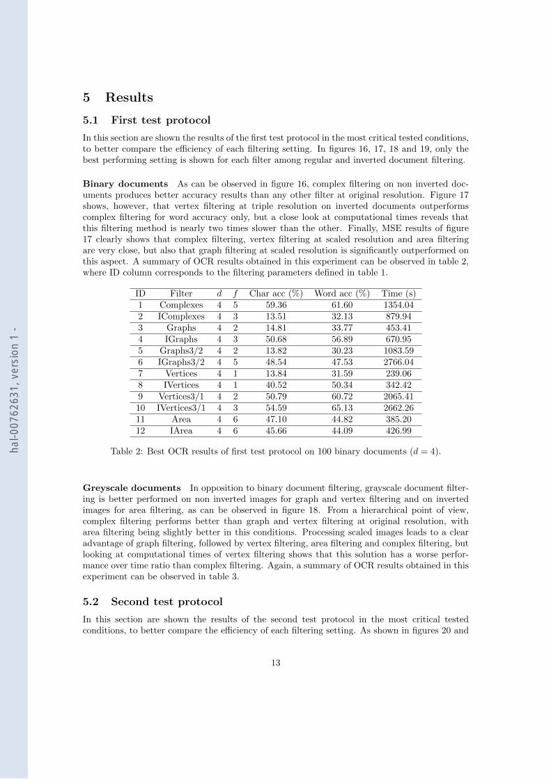
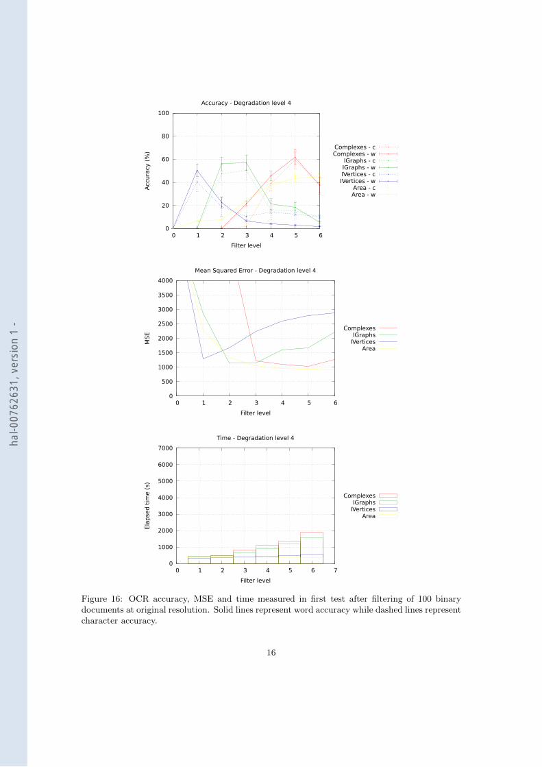
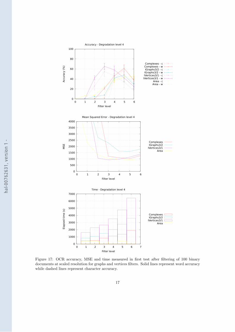
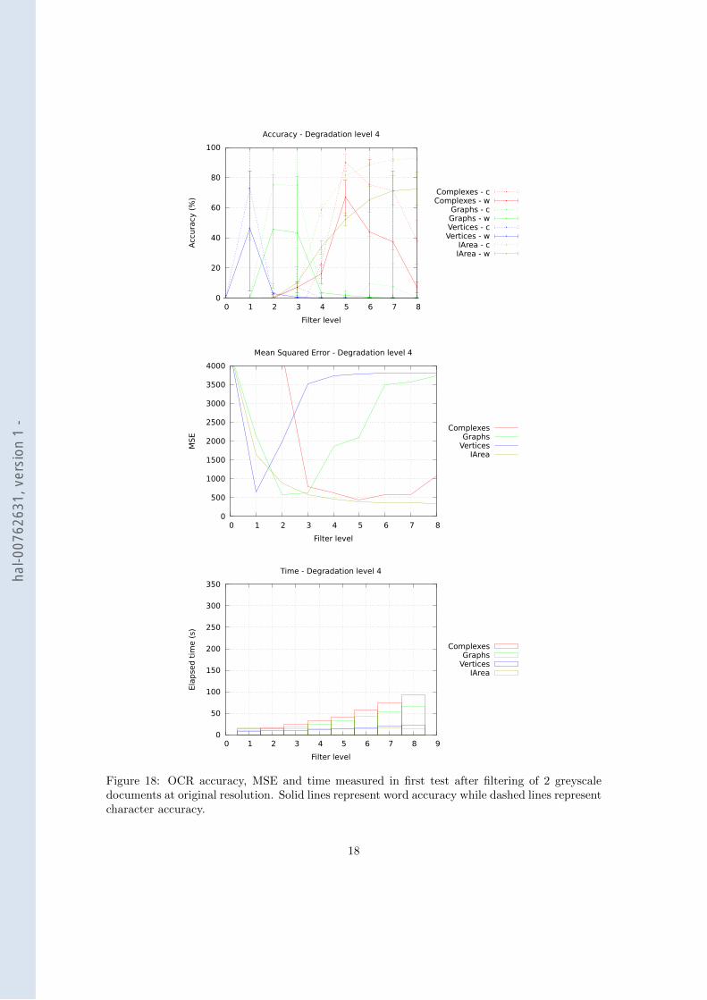
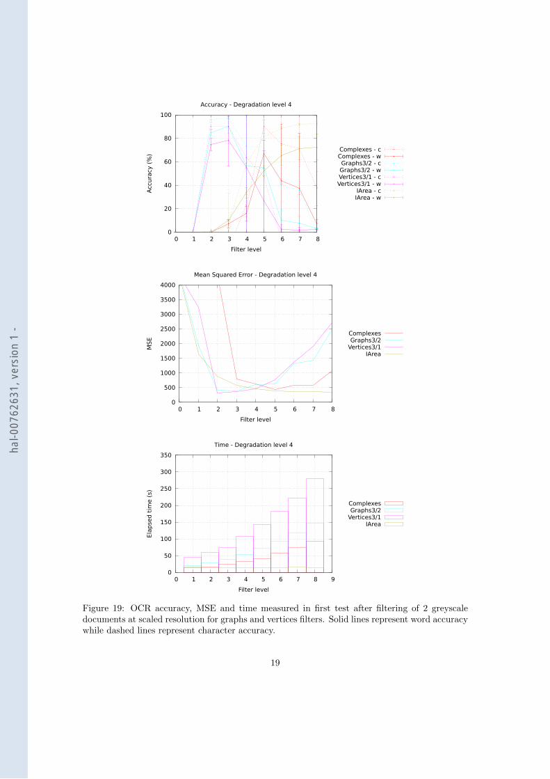
In this section are shown the results of the first test protocol in the most critical tested conditions,to better compare the efficiency of each filtering setting. In figures 16, 17, 18 and 19, only thebest performing setting is shown for each filter among regular and inverted document filtering.

Binary documents As can be observed in figure 16, complex filtering on non inverted doc-uments produces better accuracy results than any other filter at original resolution. Figure 17shows, however, that vertex filtering at triple resolution on inverted documents outperformscomplex filtering for word accuracy only, but a close look at computational times reveals thatthis filtering method is nearly two times slower than the other. Finally, MSE results of figure17 clearly shows that complex filtering, vertex filtering at scaled resolution and area filteringare very close, but also that graph filtering at scaled resolution is significantly outperformed onthis aspect. A summary of OCR results obtained in this experiment can be observed in table 2,where ID column corresponds to the filtering parameters defined in table 1.

ID Filter d f Char acc (%) Word acc (%) Time (s)1 Complexes 4 5 59.36 61.60 1354.042 IComplexes 4 3 13.51 32.13 879.943 Graphs 4 2 14.81 33.77 453.414 IGraphs 4 3 50.68 56.89 670.955 Graphs3/2 4 2 13.82 30.23 1083.596 IGraphs3/2 4 5 48.54 47.53 2766.047 Vertices 4 1 13.84 31.59 239.068 IVertices 4 1 40.52 50.34 342.429 Vertices3/1 4 2 50.79 60.72 2065.4110 IVertices3/1 4 3 54.59 65.13 2662.2611 Area 4 6 47.10 44.82 385.2012 IArea 4 6 45.66 44.09 426.99

Table 2: Best OCR results of first test protocol on 100 binary documents (d = 4).

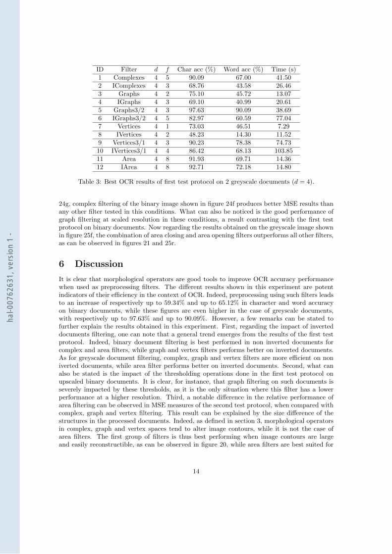
Greyscale documents In opposition to binary document filtering, grayscale document filter-ing is better performed on non inverted images for graph and vertex filtering and on invertedimages for area filtering, as can be observed in figure 18. From a hierarchical point of view,complex filtering performs better than graph and vertex filtering at original resolution, witharea filtering being slightly better in this conditions. Processing scaled images leads to a clearadvantage of graph filtering, followed by vertex filtering, area filtering and complex filtering, butlooking at computational times of vertex filtering shows that this solution has a worse perfor-mance over time ratio than complex filtering. Again, a summary of OCR results obtained in thisexperiment can be observed in table 3.

5.2 Second test protocol

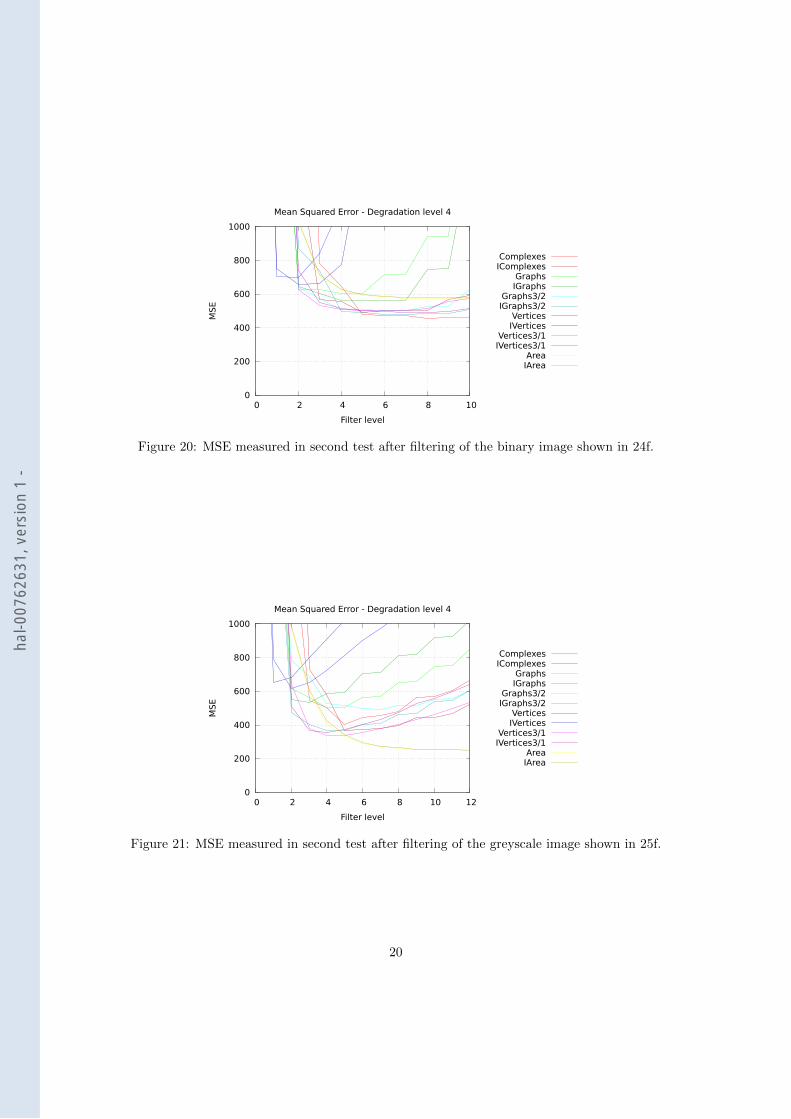
In this section are shown the results of the second test protocol in the most critical testedconditions, to better compare the efficiency of each filtering setting. As shown in figures 20 and

13

hal-0

0762

631,

ver

sion

1 -

ID Filter d f Char acc (%) Word acc (%) Time (s)1 Complexes 4 5 90.09 67.00 41.502 IComplexes 4 3 68.76 43.58 26.463 Graphs 4 2 75.10 45.72 13.074 IGraphs 4 3 69.10 40.99 20.615 Graphs3/2 4 3 97.63 90.09 38.696 IGraphs3/2 4 5 82.97 60.59 77.047 Vertices 4 1 73.03 46.51 7.298 IVertices 4 2 48.23 14.30 11.529 Vertices3/1 4 3 90.23 78.38 74.7310 IVertices3/1 4 4 86.42 68.13 103.8511 Area 4 8 91.93 69.71 14.3612 IArea 4 8 92.71 72.18 14.80

Table 3: Best OCR results of first test protocol on 2 greyscale documents (d = 4).

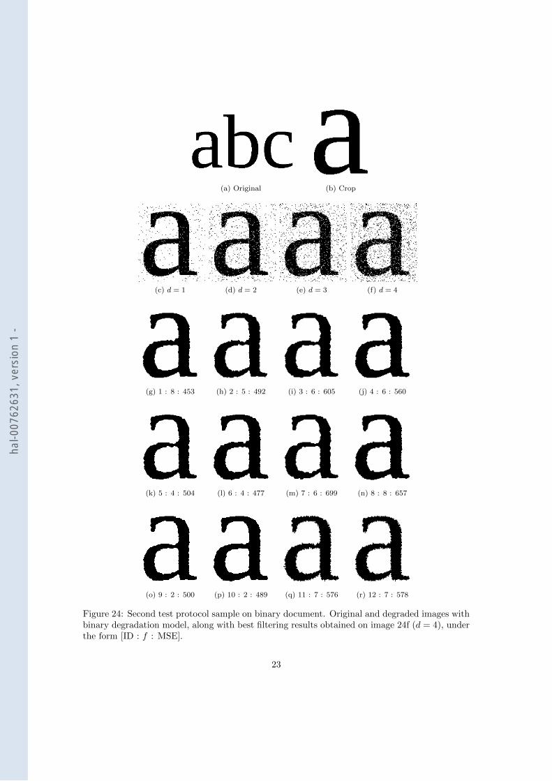
24g, complex filtering of the binary image shown in figure 24f produces better MSE results thanany other filter tested in this conditions. What can also be noticed is the good performance ofgraph filtering at scaled resolution in these conditions, a result contrasting with the first testprotocol on binary documents. Now regarding the results obtained on the greyscale image shownin figure 25f, the combination of area closing and area opening filters outperforms all other filters,as can be observed in figures 21 and 25r.

6 Discussion

It is clear that morphological operators are good tools to improve OCR accuracy performancewhen used as preprocessing filters. The different results shown in this experiment are potentindicators of their efficiency in the context of OCR. Indeed, preprocessing using such filters leadsto an increase of respectively up to 59.34% and up to 65.12% in character and word accuracyon binary documents, while these figures are even higher in the case of greyscale documents,with respectively up to 97.63% and up to 90.09%. However, a few remarks can be stated tofurther explain the results obtained in this experiment. First, regarding the impact of inverteddocuments filtering, one can note that a general trend emerges from the results of the first testprotocol. Indeed, binary document filtering is best performed in non inverted documents forcomplex and area filters, while graph and vertex filters performs better on inverted documents.As for greyscale document filtering, complex, graph and vertex filters are more efficient on noniverted documents, while area filter performs better on inverted documents. Second, what canalso be stated is the impact of the thresholding operations done in the first test protocol onupscaled binary documents. It is clear, for instance, that graph filtering on such documents isseverely impacted by these thresholds, as it is the only situation where this filter has a lowerperformance at a higher resolution. Third, a notable difference in the relative performance ofarea filtering can be observed in MSE measures of the second test protocol, when compared withcomplex, graph and vertex filtering. This result can be explained by the size difference of thestructures in the processed documents. Indeed, as defined in section 3, morphological operatorsin complex, graph and vertex spaces tend to alter image contours, while it is not the case ofarea filters. The first group of filters is thus best performing when image contours are largeand easily reconstructible, as can be observed in figure 20, while area filters are best suited for

14

hal-0

0762

631,

ver

sion

1 -

small structures that suffer from strong contour alteration (figure 21). Finally, as a concludingremark and following the previous statement, each filter have its own strengths and weaknesses.Nevertheless, complex filtering seems to be a good choice when preprocessing binary documentswith fairly large structures, while area filtering performs better on greyscale documents withsmall structures.

References

[1] Jean Cousty, Laurent Najman, and Jean Serra. Some morphological operators in graphspaces. In Mathematical Morphology and Its Application to Signal and Image Processing -Proceedings of the 9th International Symposium on Mathematical Morphology (ISMM 2009),volume 5720 of Lecture Notes in Computer Science, pages 149–160, Groningen, The Nether-lands, aug 2009. Springer Berlin / Heidelberg.

[2] Fabio Dias, Jean Cousty, and Laurent Najman. Some morphological operators on simplicialcomplex spaces. In Discrete Geometry for Computer Imagery - Proceedings of the 16th IAPRInternational Conference (DGCI 2011), volume 6607 of Lecture Notes in Computer Science,pages 441–452, Nancy, France, apr 2011. Springer Berlin / Heidelberg.

[3] Tapas Kanungo, Robert M. Haralick, Henry S. Baird, Werner Stuezle, and David Madigan.A statistical, nonparametric methodology for document degradation model validation. IEEETransactions on Pattern Analysis and Machine Intelligence, 22(11):1209–1223, nov 2000.

[4] Thomas A. Nartker, Stephen V. Rice, and Frank R. Jenkins. Ocr accuracy: Unlv’s fourthannual test. Inform, 9(7):38–46, jul 1995.

[5] Thomas A. Nartker, Stephen V. Rice, and Steven E. Lumos. Software tools and test datafor research and testing of page-reading ocr systems. In Document Recognition and RetrievalXII, volume 5676 of Proceedings of SPIE, pages 37–47, San Jose, CA, USA, jan 2005. SPIE.

[6] Ray Smith. An overview of the tesseract ocr engine. In Proceedings of the 9th InternationalConference on Document Analysis and Recognition (ICDAR 2007), volume 2, pages 629–633,Curitiba, Parana, Brazil, sep 2007. IEEE.

[7] Luc Vincent. Morphological area openings and closings for greyscale images. In Shape inPicture, volume 126 of Nato ASI Series, pages 197–208, Driebergen, The Netherlands, sep1992. Springer Berlin / Heidelberg.

15

hal-0

0762

631,

ver

sion

1 -

0

20

40

60

80

100

0 1 2 3 4 5 6

Acc

ura

cy (

%)

Filter level

Accuracy - Degradation level 4

Complexes - cComplexes - w

IGraphs - cIGraphs - wIVertices - cIVertices - w

Area - cArea - w

0

500

1000

1500

2000

2500

3000

3500

4000

0 1 2 3 4 5 6

MSE

Filter level

Mean Squared Error - Degradation level 4

ComplexesIGraphs

IVerticesArea

0

1000

2000

3000

4000

5000

6000

7000

0 1 2 3 4 5 6 7

Ela

pse

d t

ime (

s)

Filter level

Time - Degradation level 4

ComplexesIGraphs

IVerticesArea

Figure 16: OCR accuracy, MSE and time measured in first test after filtering of 100 binarydocuments at original resolution. Solid lines represent word accuracy while dashed lines representcharacter accuracy.

16

hal-0

0762

631,

ver

sion

1 -

0

20

40

60

80

100

0 1 2 3 4 5 6

Acc

ura

cy (

%)

Filter level

Accuracy - Degradation level 4

Complexes - cComplexes - wIGraphs3/2 - cIGraphs3/2 - wIVertices3/1 - cIVertices3/1 - w

Area - cArea - w

0

500

1000

1500

2000

2500

3000

3500

4000

0 1 2 3 4 5 6

MSE

Filter level

Mean Squared Error - Degradation level 4

ComplexesIGraphs3/2

IVertices3/1Area

0

1000

2000

3000

4000

5000

6000

7000

0 1 2 3 4 5 6 7

Ela

pse

d t

ime (

s)

Filter level

Time - Degradation level 4

ComplexesIGraphs3/2

IVertices3/1Area

Figure 17: OCR accuracy, MSE and time measured in first test after filtering of 100 binarydocuments at scaled resolution for graphs and vertices filters. Solid lines represent word accuracywhile dashed lines represent character accuracy.

17

hal-0

0762

631,

ver

sion

1 -

0

20

40

60

80

100

0 1 2 3 4 5 6 7 8

Acc

ura

cy (

%)

Filter level

Accuracy - Degradation level 4

Complexes - cComplexes - w

Graphs - cGraphs - wVertices - cVertices - w

IArea - cIArea - w

0

500

1000

1500

2000

2500

3000

3500

4000

0 1 2 3 4 5 6 7 8

MSE

Filter level

Mean Squared Error - Degradation level 4

ComplexesGraphs

VerticesIArea

0

50

100

150

200

250

300

350

0 1 2 3 4 5 6 7 8 9

Ela

pse

d t

ime (

s)

Filter level

Time - Degradation level 4

ComplexesGraphs

VerticesIArea

Figure 18: OCR accuracy, MSE and time measured in first test after filtering of 2 greyscaledocuments at original resolution. Solid lines represent word accuracy while dashed lines representcharacter accuracy.

18

hal-0

0762

631,

ver

sion

1 -

0

20

40

60

80

100

0 1 2 3 4 5 6 7 8

Acc

ura

cy (

%)

Filter level

Accuracy - Degradation level 4

Complexes - cComplexes - wGraphs3/2 - cGraphs3/2 - wVertices3/1 - cVertices3/1 - w

IArea - cIArea - w

0

500

1000

1500

2000

2500

3000

3500

4000

0 1 2 3 4 5 6 7 8

MSE

Filter level

Mean Squared Error - Degradation level 4

ComplexesGraphs3/2

Vertices3/1IArea

0

50

100

150

200

250

300

350

0 1 2 3 4 5 6 7 8 9

Ela

pse

d t

ime (

s)

Filter level

Time - Degradation level 4

ComplexesGraphs3/2

Vertices3/1IArea

Figure 19: OCR accuracy, MSE and time measured in first test after filtering of 2 greyscaledocuments at scaled resolution for graphs and vertices filters. Solid lines represent word accuracywhile dashed lines represent character accuracy.

19

hal-0

0762

631,

ver

sion

1 -

0

200

400

600

800

1000

0 2 4 6 8 10

MSE

Filter level

Mean Squared Error - Degradation level 4

ComplexesIComplexes

GraphsIGraphs

Graphs3/2IGraphs3/2

VerticesIVertices

Vertices3/1IVertices3/1

AreaIArea

Figure 20: MSE measured in second test after filtering of the binary image shown in 24f.

0

200

400

600

800

1000

0 2 4 6 8 10 12

MSE

Filter level

Mean Squared Error - Degradation level 4

ComplexesIComplexes

GraphsIGraphs

Graphs3/2IGraphs3/2

VerticesIVertices

Vertices3/1IVertices3/1

AreaIArea

Figure 21: MSE measured in second test after filtering of the greyscale image shown in 25f.

20

hal-0

0762

631,

ver

sion

1 -

(a) Original (b) Crop (c) d = 1 (d) d = 2

(e) d = 3 (f) d = 4 (g) 1 : 5 (h) 4 : 3

(i) 6 : 5 (j) 8 : 1 (k) 10 : 3 (l) 11 : 6

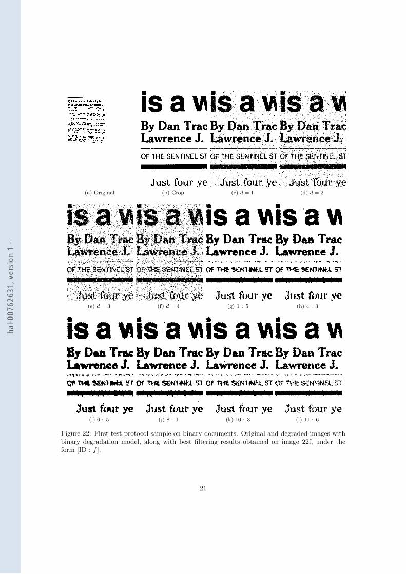
Figure 22: First test protocol sample on binary documents. Original and degraded images withbinary degradation model, along with best filtering results obtained on image 22f, under theform [ID : f ].

21

hal-0

0762

631,

ver

sion

1 -

(a) Original (b) Crop (c) d = 1 (d) d = 2

(e) d = 3 (f) d = 4 (g) 1 : 5 (h) 3 : 2

(i) 5 : 3 (j) 7 : 1 (k) 9 : 3 (l) 12 : 8

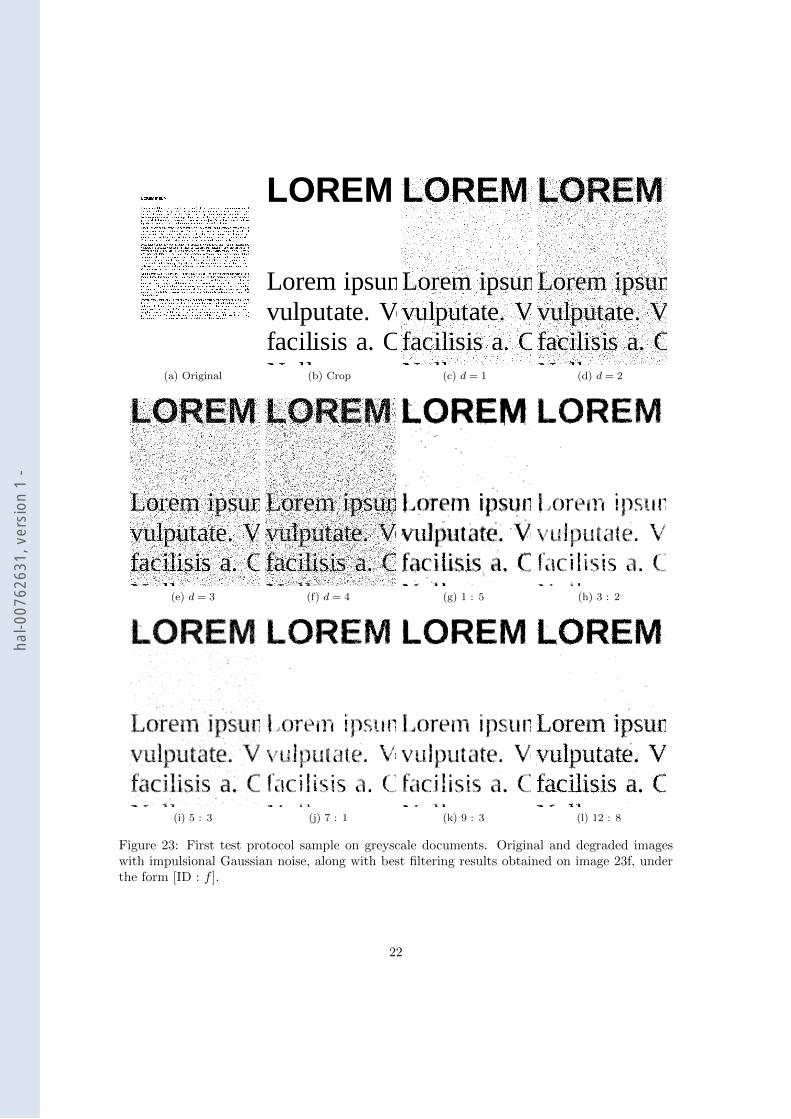
Figure 23: First test protocol sample on greyscale documents. Original and degraded imageswith impulsional Gaussian noise, along with best filtering results obtained on image 23f, underthe form [ID : f ].

22

hal-0

0762

631,

ver

sion

1 -

(a) Original (b) Crop

(c) d = 1 (d) d = 2 (e) d = 3 (f) d = 4

(g) 1 : 8 : 453 (h) 2 : 5 : 492 (i) 3 : 6 : 605 (j) 4 : 6 : 560

(k) 5 : 4 : 504 (l) 6 : 4 : 477 (m) 7 : 6 : 699 (n) 8 : 8 : 657

(o) 9 : 2 : 500 (p) 10 : 2 : 489 (q) 11 : 7 : 576 (r) 12 : 7 : 578

Figure 24: Second test protocol sample on binary document. Original and degraded images withbinary degradation model, along with best filtering results obtained on image 24f (d = 4), underthe form [ID : f : MSE].

23

hal-0

0762

631,

ver

sion

1 -

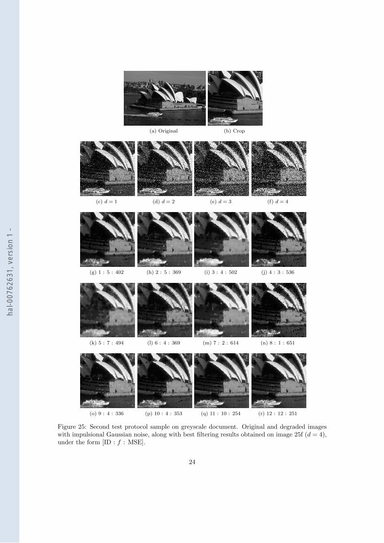
(a) Original (b) Crop

(c) d = 1 (d) d = 2 (e) d = 3 (f) d = 4

(g) 1 : 5 : 402 (h) 2 : 5 : 369 (i) 3 : 4 : 502 (j) 4 : 3 : 536

(k) 5 : 7 : 494 (l) 6 : 4 : 369 (m) 7 : 2 : 614 (n) 8 : 1 : 651

(o) 9 : 4 : 336 (p) 10 : 4 : 353 (q) 11 : 10 : 254 (r) 12 : 12 : 251

Figure 25: Second test protocol sample on greyscale document. Original and degraded imageswith impulsional Gaussian noise, along with best filtering results obtained on image 25f (d = 4),under the form [ID : f : MSE].

24

hal-0

0762

631,

ver

sion

1 -