Mostly Planar Motion

John E. Hurtado

Department of Aerospace Engineering

Texas A&M University, College Station

A complete set of notes and examples for a one-semester, sophomore-level

dynamics course. Broadly speaking, the content covers point mass and rigid

body dynamics in the plane, elementary orbital motions, and elementary rocket

dynamics. The principles are presented in a rigorous manner and problems are

approached in a systematic way. Furthermore, the notes follow my usual 1-page,

1-topic style.

ii

Preface. This is a thin companion to many sophomore-level dynamics texts.

Although this set of notes cannot replace a full-°edged text, its concise form

may make it useful for quick reference. My preferences in content and style are

re°ected in the material and its presentation.

In keeping with a sophomore-level treatment, I've constrained this mate-

rial in two signi¯cant ways. Firstly, only planar motions are covered. (The

sole exception is 3-D kinematics using cylindrical coordinates, which could be

overlooked.) My reason for keeping things planar is that almost all of the fun-

damental tools and techniques that are needed to study advanced dynamics can

be learned within planar motions. Secondly, there is no mention or use of dif-

ferential equation techniques to compute solutions to the governing equations.

My reason is that the subject of di®erential equations is beyond the grasp of

most sophomore-level students, and it's not needed to understand the evolution

of many basic systems.

Certain areas of mathematics are essential to master a subject like dynamics.

Particularly, algebra and calculus skills are needed to e±ciently and e®ectively

develop and investigate the equations that govern motion. Another essential

skill, which is important to engineering in general, is the ability to properly set-

up assigned problems; that is, to transform an inquiry into precise mathematical

statements. Hopefully, these notes will help a student develop and hone all of

these skills.

Finally, note that a ? followed by a number (e.g. ? 1) indicates an example

or an exercise.

JEH

June 7, 2010

For Juan Sandez and Linda Ann

iv

References and Supplemental Sources. Meriam and Kraige's text is suit-

able for a sophomore-level dynamics course.

Barger, V. & Olsson M. 1995 Classical Mechanics: A Modern Perspective. New

York, New York: McGraw-Hill Companies.

Beer, F.P. & Johnston E.R. 2004 Vector Mechanics for Engineers: Statics and

Dynamics, 7ed. New York, New York: McGraw-Hill Companies.

Greenwood, D.T 1988 Principles of Dynamics, 2ed. Englewood Cli®s, New

Jersey: Prentice-Hall.

? Meriam, J.L. & Kraige, L.G. 2007 Engineering Mechanics: Dynamics, 6ed.

John Wiley and Sons, Inc.

Nelson, E.W., Best, C.L. & McLean, W.G. 1997 Schaum's Outline of Engineer-

ing Mechanics. New York, New York: McGraw-Hill Companies.

Thomson, W.T. 1986 Introduction to Space Dynamics. Mineola, New York:

Dover Publications.

Wiesel, W.E. 1989 Space°ight Dynamics. New York, New York: McGraw-Hill

Companies.

v

Contents

Preface. . . . . . . . . . . . . . . . . . . . . . . . . . . . . ii

References and Supplemental Sources. . . . . . . . . . . . iv

1 Preliminaries 1

An Introduction. . . . . . . . . . . . . . . . . . . . . . . . 2

The Parts of Engineering Mechanics. . . . . . . . . . . . . 3

Kinematics & Kinetics. . . . . . . . . . . . . . . . . . . . 4

Di®erent Types of Vectors. . . . . . . . . . . . . . . . . . 5

Frames of Reference. . . . . . . . . . . . . . . . . . . . . . 6

Coordinate Systems. . . . . . . . . . . . . . . . . . . . . . 7

Newton's Laws. . . . . . . . . . . . . . . . . . . . . . . . . 8

2 Point Mass Kinematics in Stationary Frames 9

An Introduction. . . . . . . . . . . . . . . . . . . . . . . . 10

Rectilinear Motion. . . . . . . . . . . . . . . . . . . . . . . 11

? 1 Descent of a Lunar Lander. . . . . . . . . . . . . . . . 12

? 2 Escape Velocity. . . . . . . . . . . . . . . . . . . . . . 13

? 3 Escape Altitude. . . . . . . . . . . . . . . . . . . . . . 14

Constant Acceleration & Distance Traveled. . . . . . . . . 15

Planar Motion. . . . . . . . . . . . . . . . . . . . . . . . . 16

? 4 A Fired Missile. . . . . . . . . . . . . . . . . . . . . . 17

Projectile Motion. . . . . . . . . . . . . . . . . . . . . . . 18

? 5 Extremes in Projectile Motion. . . . . . . . . . . . . . 19

The Trajectory Space. . . . . . . . . . . . . . . . . . . . . 20

? 6 Trajectory Envelope Computations. . . . . . . . . . . 21

A Down Range Plot. . . . . . . . . . . . . . . . . . . . . . 22

Notes. . . . . . . . . . . . . . . . . . . . . . . . . . . . . . 23

3 Point Mass Kinematics using Rotating Frames 24

An Introduction. . . . . . . . . . . . . . . . . . . . . . . . 25

vi

Rotating Reference Frames. . . . . . . . . . . . . . . . . . 26

Relating One Set of Unit Vectors to Another. . . . . . . . 27

? 7 A Two-Link Robot Arm. . . . . . . . . . . . . . . . . 28

Planar Kinematics in Polar Coordinates. . . . . . . . . . . 29

? 8 Radar Tracking of a Rocket. . . . . . . . . . . . . . . 30

Normal and Tangential Velocity Coordinates. . . . . . . . 31

A Collection of Kinematic Coordinates. . . . . . . . . . . 32

Satellite Speed in a Circular Orbit. . . . . . . . . . . . . . 33

Cylindrical Coordinates for Motion in 3-D. . . . . . . . . 34

? 9 The Spiraling Descent of a Glider. . . . . . . . . . . . 35

Notes. . . . . . . . . . . . . . . . . . . . . . . . . . . . . . 36

4 Point Mass Kinetics in Stationary Frames 37

An Introduction. . . . . . . . . . . . . . . . . . . . . . . . 38

Newton's Second Law: N2L. . . . . . . . . . . . . . . . . 39

A Point Mass Routine. . . . . . . . . . . . . . . . . . . . . 40

? 10 A Block on an Inclined Plane. . . . . . . . . . . . . . 41

? 11 A Block on an Inclined Plane II. . . . . . . . . . . . 42

? 12 A Collar on a Shaft. . . . . . . . . . . . . . . . . . . 43

Equations of Motion: Now What? . . . . . . . . . . . . . 44

? 13 A Model Rocket Problem. . . . . . . . . . . . . . . . 45

? 14 The Archer's Bow. . . . . . . . . . . . . . . . . . . . 46

? 15 A Point Mass Lunar Rocket. . . . . . . . . . . . . . . 47

? 16 A Point Mass in a Thick Fluid. . . . . . . . . . . . . 48

? 17 The Sky Diver. . . . . . . . . . . . . . . . . . . . . . 49

Euler's Simple, Simple Numerical Integration. . . . . . . . 50

? 18 An Euler Numerical Integration Picture. . . . . . . . 51

Rigidly Connected Bodies. . . . . . . . . . . . . . . . . . . 52

? 19 Two Blocks. . . . . . . . . . . . . . . . . . . . . . . . 53

? 20 A Toy Train. . . . . . . . . . . . . . . . . . . . . . . 55

? 21 A Hanging Chain. . . . . . . . . . . . . . . . . . . . 57

vii

Integrated Or Momentum Form. . . . . . . . . . . . . . . 58

? 22 Cart Momentum. . . . . . . . . . . . . . . . . . . . . 59

Notes. . . . . . . . . . . . . . . . . . . . . . . . . . . . . . 60

5 A Sticky Situation 61

An Introduction. . . . . . . . . . . . . . . . . . . . . . . . 62

General Friction Scenarios. . . . . . . . . . . . . . . . . . 63

? 23 The Friction Illustrations. . . . . . . . . . . . . . . . 64

Known Impending Motion. . . . . . . . . . . . . . . . . . 65

? 24 Known Impending Motion of Stacked Blocks. . . . . 66

? 25 Known Sliding Motion of Stacked Blocks. . . . . . . 67

? 26 Known Impending Motion of a Hanging Chain. . . . 68

? 27 Known Sliding Motion of a Hanging Chain. . . . . . 69

? 28 Another Known Sliding Motion Example. . . . . . . 71

Will Motion Occur? . . . . . . . . . . . . . . . . . . . . . 73

? 29 A Block Worked Two Ways. . . . . . . . . . . . . . . 74

Notes. . . . . . . . . . . . . . . . . . . . . . . . . . . . . . 77

6 Point Mass Kinetics using Rotating Frames 78

An Introduction. . . . . . . . . . . . . . . . . . . . . . . . 79

A Motivating Example. . . . . . . . . . . . . . . . . . . . 80

? 30 Simple Pendulum Equations in a Fixed Reference

Frame. . . . . . . . . . . . . . . . . . . . . . . . 81

? 31 Simple Pendulum Equations in a Rotating Reference

Frame. . . . . . . . . . . . . . . . . . . . . . . . 82

A Di®erence Between Linear and Nonlinear Equations. . . 83

? 32 The Vomit Comet. . . . . . . . . . . . . . . . . . . . 84

? 33 An Airplane Loop. . . . . . . . . . . . . . . . . . . . 85

? 34 The Swinging Pendulum. . . . . . . . . . . . . . . . . 86

? 35 The Block Slides O® the Dome. . . . . . . . . . . . . 87

? 36 The Block Slides Down the Bowl. . . . . . . . . . . . 88

viii

? 37 Satellite in Elliptic Orbit. . . . . . . . . . . . . . . . 90

Notes. . . . . . . . . . . . . . . . . . . . . . . . . . . . . . 92

7 Point Mass Angular Momentum 93

An Introduction. . . . . . . . . . . . . . . . . . . . . . . . 94

The De¯nition. . . . . . . . . . . . . . . . . . . . . . . . . 95

? 38 A Point Mass Launched o® a Table. . . . . . . . . . 96

The Time Derivative of ho. . . . . . . . . . . . . . . . . . 97

? 39 _ho for the Point Mass Launched o® a Table. . . . . . 98

The Mutual Attraction of Two Bodies. . . . . . . . . . . . 99

? 40 Development of the Relative 2-Body Equations. . . . 100

Angular Momentum of the Relative 2-Body Problem. . . 101

Presto Chango for the Relative 2-Body Problem. . . . . . 102

? 41 A Presto Chango Exercise. . . . . . . . . . . . . . . . 103

Energy of the Relative 2-Body Problem. . . . . . . . . . . 104

(One More Integration Reveals Conic Sections.) . . . . . . 105

? 42 Relative 2-Body Motion. . . . . . . . . . . . . . . . . 107

Notes. . . . . . . . . . . . . . . . . . . . . . . . . . . . . . 108

8 Rigid Body Kinematics 109

An Introduction. . . . . . . . . . . . . . . . . . . . . . . . 110

Position and Attitude. . . . . . . . . . . . . . . . . . . . . 111

Body-Fixed Reference Frames. . . . . . . . . . . . . . . . 112

Velocities: Speci¯cally, What is Angular Velocity? . . . . 113

Translational and Rotational Acceleration. . . . . . . . . 114

? 43 Looping Maneuver of a Rigid Body Airplane. . . . . 115

(An Angular Position Vector?) . . . . . . . . . . . . . . . 116

Position and Velocity of Two Points on the Same Body. . 117

? 44 Velocities of a Sliding Rod. . . . . . . . . . . . . . . 118

? 45 Revolution and Rotation of the Moon. . . . . . . . . 119

Acceleration of Two Points on the Same Rigid Body. . . . 120

ix

? 46 Accelerations of a Sliding Rod. . . . . . . . . . . . . 121

Rotational Motion Only. . . . . . . . . . . . . . . . . . . . 122

? 47 A Rotating Disk. . . . . . . . . . . . . . . . . . . . . 123

Kinematics of Roll Without Slip. . . . . . . . . . . . . . . 124

Roll Without Slip Accelerations. . . . . . . . . . . . . . . 125

? 48 A Disk Rolls on a Dome. . . . . . . . . . . . . . . . . 126

? 49 A Disk Rolls in a Bowl. . . . . . . . . . . . . . . . . 128

Notes. . . . . . . . . . . . . . . . . . . . . . . . . . . . . . 129

9 Rigid Body Kinetics 130

An Introduction. . . . . . . . . . . . . . . . . . . . . . . . 131

Newton and Euler. . . . . . . . . . . . . . . . . . . . . . . 132

A First Look at Angular Momentum. . . . . . . . . . . . 133

? 50 Showing the Translation Theorem for Angular Mo-

mentum. . . . . . . . . . . . . . . . . . . . . . . 134

A Collection of Newton and Euler Laws. . . . . . . . . . . 135

Introducing Inertia. . . . . . . . . . . . . . . . . . . . . . 136

? 51 Rigid Body Inertia in the Plane. . . . . . . . . . . . 137

? 52 Planar Inertia of Common Shapes. . . . . . . . . . . 138

The Useful Collection of Newton and Euler Laws. . . . . 139

A Rigid Body Routine. . . . . . . . . . . . . . . . . . . . 140

? 53 A Swinging Rod. . . . . . . . . . . . . . . . . . . . . 141

Parallel Axis Theorem and Radius of Gyration. . . . . . . 143

? 54 General Planar Motion of a Rod. . . . . . . . . . . . 144

? 55 Two Rigid Bodies. . . . . . . . . . . . . . . . . . . . 146

Will the Wheel Slide? . . . . . . . . . . . . . . . . . . . . 149

? 56 Pulling on a Disk. . . . . . . . . . . . . . . . . . . . . 150

? 57 The `Backspinning' Ball. . . . . . . . . . . . . . . . . 152

(Hula Hoops and Bowling Balls). . . . . . . . . . . . . . . 154

Notes. . . . . . . . . . . . . . . . . . . . . . . . . . . . . . 155

x

10 Energy Analysis 156

An Introduction. . . . . . . . . . . . . . . . . . . . . . . . 157

Kinetic Energy of a Point Mass. . . . . . . . . . . . . . . 158

? 58 Kinetic Energy of a Sliding Block. . . . . . . . . . . 159

Potential Forces. . . . . . . . . . . . . . . . . . . . . . . . 160

Total Energy. . . . . . . . . . . . . . . . . . . . . . . . . . 161

? 59 Total Energy of an Inclined Block. . . . . . . . . . . 162

Energy of a Rigid Body. . . . . . . . . . . . . . . . . . . . 163

? 60 The Compound Pendulum. . . . . . . . . . . . . . . 164

The Change in Energy of a Rigid Body. . . . . . . . . . . 165

? 61 Martian Rover Deployment. . . . . . . . . . . . . . . 166

Notes. . . . . . . . . . . . . . . . . . . . . . . . . . . . . . 168

11 Docking, Despin, & Thrust 169

An Introduction. . . . . . . . . . . . . . . . . . . . . . . . 170

A Momentum Analysis for Docking. . . . . . . . . . . . . 171

? 62 Command and Lunar Module Docking. . . . . . . . 172

Energy Lost in Docking. . . . . . . . . . . . . . . . . . . . 173

Satellite Despin. . . . . . . . . . . . . . . . . . . . . . . . 174

? 63 Yo-yo Despin. . . . . . . . . . . . . . . . . . . . . . . 175

An Instantaneous Form. . . . . . . . . . . . . . . . . . . . 176

The Sounding Rocket. . . . . . . . . . . . . . . . . . . . . 177

Single Stage to Orbit. . . . . . . . . . . . . . . . . . . . . 178

(? 64 Variable Mass Rocket Exercises.) . . . . . . . . . . . 179

(Achieving Exhaust Velocity Speed & More.) . . . . . . . 180

(Maximum Altitude.) . . . . . . . . . . . . . . . . . . . . 181

Notes. . . . . . . . . . . . . . . . . . . . . . . . . . . . . . 182

1 Preliminaries

2

An Introduction. This ¯rst chapter is used to introduce some of the main

concepts that are a part of the principles of motion. These include the di®erences

between kinematics and kinetics, the di®erences in the types of vectors that

are used to model physical entities, the characteristics of reference frames and

coordinate systems, and Newton's laws of motion. This material is commonly

found in the beginning pages of dynamics textbooks, e.g., chapter 1 of Meriam

and Kraige.

3

The Parts of Engineering Mechanics.1 Engineering mechanics is typically

divided into three branches.

1. Mechanics of point mass models and rigid bodies: this topic deals with

external forces and moments acting on the surface or boundary of rigid

bodies or point mass models. Point mass models and rigid body models

are truly only idealizations.

2. Mechanics of deformable bodies: this topic deals with internal force dis-

tributions and deformations that occur when bodies are subject to forces

and moments. All real engineering structures are deformable. Sometimes

rigid body assumptions are valid or acceptable and sometimes they are

not. This material is also commonly called mechanics of materials.

3. Mechanics of °uids: this topic deals with liquids and gases at rest or in

motion. More simply, this topic is called °uid mechanics. Fluids can be

further modeled as being compressible or incompressible, and this depends

on whether the °uid density varies with temperature, pressure, etc.

1Paraphrased from notes of W.E. Haisler.

4

Kinematics & Kinetics. Each one of the branches or areas of engineering

mechanics can be further divided into two topics.

1. Kinematics: this topic is concerned with the appearance of motion. The

focus is on describing motion without regard to why motion is occuring.

Kinematics analysis can provide relationships between position, velocity,

and acceleration. Kinematics involves geometry alone and has nothing to

do with the laws (Newton's or Euler's) of motion. Therefore, this topic is

sometimes referred to as the geometry of motion.

2. Kinetics: this topic deals with bodies subject to forces and moments.

Forces and moments can make a body accelerate or not. In the acceleration

case it is sometimes said that the forces and moments are unbalanced;

conversely, in the zero acceleration case it is sometimes said that the forces

and moments are balanced. Traditionally, the unbalanced case is called the

dynamics problem whereas the balanced case is called the statics problem.

The laws of motion (Newton's or Euler's) have everything to do with the

kinetics situation.

5

Di®erent Types of Vectors. Vectors and scalars are central to studying the

principles of motion because motion itself, the forces that cause motion, and the

object properties that participate in motion can be represented by them. We

know what a vector is and that, from a mathematical point of view, magnitude

and direction are the important vector quantities. But vectors can represent

physical quantities and sometimes the physical quantities have an added impor-

tance related to the location of the vector. This gives rise to classi¯cations like

free vectors, sliding vectors, and bound vectors.

A free vector has magnitude and direction but no speci¯ed location or point

of application. For example, the angular velocity of a rigid body is a free vector.

So is a pure torque applied to a rigid body.2

A sliding vector has magnitude, direction, and a line of action that is aligned

with the vector direction. The relevant point is that the a®ect of the vector is

the same regardless of where the vector is placed along the line of action. For

example, a force acting on a rigid body is a sliding vector because its in°uence

on the overall motion (translational and rotational) is independent of where the

vector is placed along the line of action. (This truth regarding rigid body forces

is called the principle of transmissibility.)

A bound vector has magnitude, direction, and a precise point of application.

An applied force on an elastic body is an example of a bound vector.

Operations on vectors are most meaningful when they are explicitly carried

out using vector components. But in order to discuss vector components, we

must ¯rst introduce reference frames and coordinate systems.

2Truthfully, these free vectors are planar entities. Angular velocity is really angular velocity

in a plane. And a pure torque is really pure torque in a plane. We are able to dress these planar

entities as vectors because of the vector-plane equivalency that exists in three dimensions.

6

Frames of Reference. A frame of reference (or reference frame) is de¯ned as

a collection of points such that the distance between the points is constant with

respect to time. The minimum number of points required to de¯ne a reference

frame in three-dimensional space is three noncollinear points. A reference frame

is used to make observations regarding motion, but it does not provide a way

to measure the motion. (For that, we must introduce a coordinate system.)

Reference frames can be inertial or non-inertial. An inertial reference frame

is one whose points are either absolutely ¯xed in space or at most translate

relative to an absolutely ¯xed set of points with the same constant velocity. A

non-inertial reference frame is one whose points accelerate with time.

Inertial reference frames are important because it is an axiom of Newtonian

mechanics that such frames exist and that his laws of mechanics are valid only

in such frames.

7

Coordinate Systems. A coordinate system can be overlayed on a reference

frame. Indeed, a reference frame can be home to an in¯nite number of coordinate

systems, but typically one associates one reference frame to one coordinate

system and the two become synonymous.

A coordinate system is a group of objects within a reference frame that

allows measurement. In three-dimensional space, the system is constructed by

three mutually orthogonal unit vectors in a reference frame, called the axes

of the coordinate system or the coordinate axes or the reference vectors, that

meet at a point in a reference frame, called the origin.3 The set of unit vectors

always form a right-handed system. As an example, we could de¯ne a coordinate

system a+ to have coordinate axes ai meeting at an origin o in some reference

frame.4

a+ : fo; a1; a2; a3g or a+ : fo; aig; i = 1; 2; 3 (7.1)

We would call this coordinate system a+ in the reference frame, or because of

the close relationship between reference frames and coordinate systems, simply

the a+ frame or frame a+. Furthermore, the coordinate axes ai will often be

simply called the a+ axes.

Measurement in a reference frame is done relative to the coordinate system

(or frame) origin and along the coordinate (or frame) axes. Thus, the location of

an arbitrary point in three-dimensional space can be described by the elements

of the coordinate system. All that is needed are measures along the coordinate

axes.

p = p1a1 + p2a2 + p3a3 (7.2)

Here, the pi are scalar coe±cients of the vector p in the a+ frame. These scalar

coe±cients are commonly called the components of p or the measures of p.

3Strictly speaking, the axes don't have to meet at a point.4Right-handed means, for example, a1 £ a2 = a3. Orthogonal means ai ¢ aj = 0 if i 6= j.

And unit vector means jjaijj = 1.

8

Newton's Laws. Newton's original laws of motion may be stated using mod-

ern language in the following way.

N1L | A point mass remains at rest or continues to move with uniform

velocity, which means with constant speed along a straight line, if the

forces acting on it are balanced.

N2L | A point mass accelerates in an amount proportional to, and in the

direction of, the unbalance of forces acting on it.

N3L | The forces of action and reaction between contacting point masses

have equal magnitudes and opposite, collinear directions.

N4L | A gravitational law governs the mutual attractive force between

point masses as described by the limerick:

If ½ be the distance to O

Sir Newton said he could show

That the force of attraction

Behaves like the fraction

Of one over the square of ½

(R.M. Rosenberg)

Newton's second law (N2L) gives us f = ma where a is the acceleration

in a non accelerating reference frame. Newton's fourth law (N4L) gives us

f = Gm1m2=½2 where G is a universal constant. N2L and N4L combine to

give that the amount of gravity at the Earth's surface is g0 = Gme=R2 =

9:825m=s2. At an altitude h above the Earth's surface, the gravity behaves

according to g = g0R2=(R+ h)2.

2 Point Mass Kinematics in Stationary Frames

10

An Introduction. The purpose of this chapter is to refresh our understanding

of motion along ¯xed directions.

One important fact that often gets overlooked is that inertial kinematic vec-

tors are critical when studying dynamics. Inertial kinematic vectors encompass

inertial position vectors, inertial velocity vectors, and inertial acceleration vec-

tors. An inertial position vector is one that is measured from a ¯xed point.5 An

inertial velocity vector is the time derivative of this inertial position vector as

viewed by an inertial observer, i.e., an observer in an inertial reference frame.

An inertial acceleration vector is the time derivative of the an inertial velocity

vector as viewed by an inertial observer.

In this section, the kinematic vectors will be measured along ¯xed directions,

or measured in ¯xed reference frames. This doesn't have to be so, but it's what

we'll do for now.

5Truly, the point can move with constant velocity along a straight line.

11

Rectilinear Motion. This begins a kinematic analysis of rectilinear motion,

including position vectors, velocity vectors, and acceleration vectors.

Rectilinear motion means motion along a ¯xed, straight line. The line can

be de¯ned by an axis (e.g., the n1 axis) of an orthogonal reference frame whose

origin is located at a ¯xed point o. The instantaneous position of a point along

the axis is measured by the coordinate x.

Commonly, information about the instantaneous position (x) or velocity (v)

or acceleration (a) is given, but information about the instantaneous position or

velocity or acceleration is sought. There are ¯ve common situations to consider.

1. x(t) is known: the magnitude of the instantaneous velocity and accelera-

tion can be determined from di®erentiation.

2. v(t) is known: the magnitude of the instantaneous position and accelera-

tion can be determined from integration and di®erentiation, respectively.

3. a(t) is known: the magnitude of the instantaneous position and velocity

can be determined from integration.

4. a(x) is known: beginning with a = dv=dt, the chain rule of calculus

gives v dv = a(x) dx, which can be integrated to give v(x). Integrat-

ing dx=v(x) = dt gives an expression that relates time to position t(x),

which can be inverted to determine position as a function of time, x(t).

5. a(v) is known: beginning with a = dv=dt, we can ¯nd an expression that

relates time to velocity. Once t(v) is formally known, the expression may

be inverted to give velocity as a function of time, v(t). The position as a

function of time immediately follows.

12

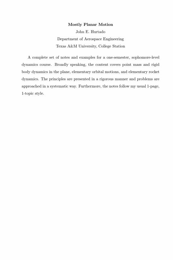
? 1 Descent of a Lunar Lander.

13

? 2 Escape Velocity.

14

? 3 Escape Altitude.

15

Constant Acceleration & Distance Traveled. Rectilinear motion involv-

ing constant acceleration is a practical, special case to consider. A familiar

example of this is the vertical motion of point mass in an idealized constant

gravity ¯eld, a = ¡9:81 m/s2. The previous results with a equal to a known

constant c are useful to ¯nd explicit expressions relating the instantaneous ve-

locity, position, and time.

v = ct+ v0 (15.1)

x =c2t2 + v0t+ x0 (15.2)

v2 = v20 + 2c(x¡ x0) (15.3)

Note that the initial time t0 is assumed to be zero in the above equations, and

that x0 and v0 are initial conditions.

When the acceleration is constant, these relationships are really all there is

to know: (15.1) gives the instantaneous velocity as a function of time, or time

as a function of velocity; (15.2) gives the instantaneous position as a function

of time, or time as a function of position; and (15.3) gives the instantaneous

velocity as a function of instantaneous position, or position as a function of

velocity.

The distance traveled by a point mass can be computed from a modi¯ed

version of x(t) =R tt0v(s) ds+ x0.

d(t) =¯¯Z t1

t0v(s) ds

¯¯+

¯¯Z t2

t1v(s) ds

¯¯+ : : :+

¯¯Z t

tn¡1

v(s) ds¯¯ (15.4)

Here, like before, t0 is the initial time. The intermediate times between t0 and

t are instances when the velocity magnitude undergoes a sign change. These

times must be identi¯ed if they are not given.

16

Planar Motion. Point mass kinematics in the plane can be studied using

Cartesian coordinates.

The instantaneous position of a point on a plane needs two independent

coordinates to pinpoint its location.

p = x n1 + y n2 (16.1)

The measures x and y can vary, but the axes n1 and n2 are ¯xed: they are unit

vectors that do not change direction.

The time derivative of the instantaneous position vector gives the instanta-

neous velocity vector, and a subsequent time derivative gives the instantaneous

acceleration vector.

v = _x n1 + _y n2 = vx n1 + vy n2

a = Äx n1 + Äy n2 = _vx n1 + _vy n2 = ax n1 + ay n2

(16.2, 16.3)

The overdot means the time derivative of the scalar measure, e.g., _x ´ dx=dt.

It is important to note that motion appears uncoupled using this Cartesian

coordinate description. That is, we could have full knowledge of x, vx, or ax

along the n1 direction and determine through di®erentiation or integration the

other unknown kinematic variables along the n1 direction. Likewise for the

kinematics along the n2 direction.

17

? 4 A Fired Missile.

18

Projectile Motion. Projectile motion is idealized motion of a point mass

near the Earth's surface. In a Cartesian coordinate description, the accelera-

tion component in the horizontal n1 direction is zero whereas the acceleration

component in the vertical n2 direction is the negative of the gravitational con-

stant. Consequently, the velocity component along the n1 direction is constant

and the position component along the n1 direction is a linear function of time.

Motion along n2 is governed by the familiar constant acceleration formulae.

Horizontal Vertical

ax = 0 v2y = v2

y0 ¡ 2g(y ¡ y0)vx = vx0 vy = ¡gt+ vy0

x = vx0t+ x0 y = ¡ 12gt

2 + vy0t+ y0

(18.1)

Often, the components of velocity are written using the launch speed and launch

angle measured from the horizon.

vx0 = v cos ° ; vy0 = v sin ° (18.2, 18.3)

These equations can be manipulated to show a few properties of projectile

motion over level terrain:

1. The range (i.e., the x component of position) is maximized for a 45 degree

launch angle;

2. The time of °ight is maximized for a 90 degree launch angle.

19

? 5 Extremes in Projectile Motion.

20

The Trajectory Space. The admissible trajectory space of projectile motion

in an unobstructed region are those (x; y) points that can be reached.

Given a launch velocity v, the admissible trajectory space is governed by a

quadratic equation in the tangent of the launch angle.

tan2 ° ¡ 2v2

gxtan ° +

µ2v2ygx2 + 1

¶= 0 (20.1)

The explicit solutions to eq. (20.1) reveal the di®erent scenarios.

tan ° =v2

gx§s

v4

g2x2 ¡2v2ygx2 ¡ 1 (20.2)

These solutions are telling: there are two launch angles for all (x; y) points

strictly inside the trajectory space, and for this case the radicand is positive;

there is only one launch angle for all (x; y) points strictly on the edge of the

trajectory space (called the trajectory envelope), and for this case the radicand

is zero; and there are nonsensical launch angles for all (x; y) points strictly

outside the trajectory space, and in this case the radicand is negative.

The trajectory envelope is de¯ned when the radicand equals zero. These are

the points that can barely be reached. Notice then, that the maximum height

of the trajectory envelope is found from setting x = 0, and the maximum range

of the trajectory envelope is found from setting y = 0.

max height y =v2

2g; max range x =

v2

g(20.3, 20.4)

Downrange

Alti

tude

Admissible Trajectory Space

Inadmissible Trajectory Space

21

? 6 Trajectory Envelope Computations.

Consider projectile motion over a °at surface. Let the launch velocity equal 100

m/s. For simplicity, let gravity equal 10 m/s2. Perform the following:

a. Show that points on the trajectory envelope are governed by a quadratic

equation.

2y = v2=g ¡ gx2=v2

b. Calculate and plot 10 points that lie on the trajectory envelope.

c. Compute the launch angles for the 10 points in part b.

d. Compute the launch angles for 3 points the lie within the trajectory en-

velope.

22

A Down Range Plot. Points in the trajectory space are governed by tan2 °¡(2v2=gx) tan °+(2v2y=gx2)+1 = 0. By setting y = 0, one can use the resulting

expression to determine the initial launch velocities and initial launch angles

that will achieve a down range distance over °at terrain. A plot of those results

are shown here. For example, for v2 = 1000 m/s2, a down range distance of 100

m can be reached for launch angles approximately equal to 40 and 50 deg. This

also shows that the maximum down range distance for a given launch velocity

will occur at 45 deg.

5

10

20

40

60

80

100

120

140

160

180200

23

Notes. This blank page is for your annotations.