Motion analysis for Arctic char and Atlantic

salmon.

Sæþór Ásgeirsson

Faculty of Mechanical Engineering University of Iceland

2013

Motion Analysis of Arctic char and Atlantic salmon

Sæþór Ásgeirsson

60 ECTS thesis submitted in partial fulfillment of a Magister Scientiarum degree in Mechanical Engineering

Advisor Rúnar Unnþórsson Halldór Pálsson

Faculty Representative Valdimar K Jónsson

Faculty of Mechanical Engineering School of Engineering and Natural Sciences

University of Iceland Reykjavik. September 2013

Motion analysis of Arctic char and Atlantic salmon. 60 ECTS thesis submitted in partial fulfillment of a Magister Scientiarum degree in Mechanical Engineering Copyright © 2013 Sæþór Ásgeirsson All rights reserved Faculty of Mechanical Engineering School of Engineering and Natural Sciences University of Iceland Hjarðarhagi 2-6 107 Reykjavik Iceland Telephone: 525 4000 Bibliographic information: Saethor Asgeirsson. 2013. Motion analysis of Arctic char and Atlantic salmon. Master’s thesis. Faculty of Engineering. University of Iceland. pp. 75 Printing: Háskólaprent ehf, Fálkagata 2, 107 Reykjavík Reykjavik. Iceland. September 2013

Abstract This thesis presents the results of a study, which aimed to understand and evaluate the locomotion of Atlantic salmon and Arctic char under three different swimming conditions, slow, medium and fast. A Fourier-series based numerical model that describes the swimming mode for each condition is presented and the control variables for a swimming fish are evaluated.

The numerical model is based on a video analysis of a swimming fish. A video recording system was used to record the movement of two fish species under different swimming conditions in a respirometer tunnel. The movements of eleven points on the fishes were tracked from the video recordings and logged. The movements of each point were then analyzed in Matlab and a model constructed to describe the motion.

Fourier series was used to determine the fish motion and mathematically important variables such as frequency, amplitude, acceleration, phase difference and the most important factor, flexibility. The change in swimming behavior of fish has not been fully understood, neither how it changes with increased swimming velocity. The change in flexibility or stiffness is addressed for sub-Carangi form type of fish and results graphically illustrated.

The conventional marine propeller has an average efficiency of about 70%. Propulsion efficiency in for example dolphins is around 90% according to F.E.Fish 1993. The possibility represents itself for a revolution in how marine vessels propel themselves with an innovative mechanical device that can replace the marine propeller.

Útdráttur Verkefni þetta snýst um að greina hreyfingar laxa og bleikju á þremur mismunandi sund hröðum. Hægt, miðlungs og hratt. Annarar gráðu Fourier röð er notuð til að lýsa hreyfingunum og niðurstöðurnar notaðar til að ákvarða hvaða breytur skipta máli í sundi þeirra.

Stærðfræðilíkan byggt á myndgreiningu af myndsbandupptöku af lax og bleikju á sundi þar sem gangapunktar staðsettir á baki fisksins eru skrásettir. Breytur eins og tíðni, útslag, hröðun, fasa munur og stífni eru reiknuð út og samanburður gerður á milli sundhraða. Stífni fiska er óþekkt breyta, þ.e.a.s. engin gögn né rannsóknir hafa verið gerðar á því hvernig stífni fiska af sub-Carangi formi breytist með auknum sundhraða. Niðurstöðurnar eru settar fram á þann hátt að auðvelt er að halda áfram þar sem frá var horfið og þróa drifkerfi fyrir báta sem líkir eftir hreyfingum fiska af sub-Carangi form.

Almennt hafa skipsskrúfur um 70% nýtni. Sundnýtni fiska er um 90% og því er möguleiki fyrir hendi að brúa bil sem gæti haft í för með sér byltingu í skipaiðnaðinum með orkusparandi drifi. Þróun og rannsóknir á drifi af þessari tegund gæti þar með opnað nýjar dyr í skipaiðnaði.

Dedication

I would like to dedicate this project to my beloved grandfather Sigurdur Gunnarsson who passed away during the course of my studies. Thank you for all the wonderful summers we spent together. I will never forget you.

ix

Table of Contents Motion Analysis of Arctic char and Atlantic salmon ........................................................ i

List of Figuress .................................................................................................................... xi

List of Tables ..................................................................................................................... xiv

Variable Names .................................................................................................................. xv

Acknowledgements .......................................................................................................... xvii

1 Introduction ................................................................................................................... 19 1.1 Motivation and objectives ..................................................................................... 19 1.2 Contributions and results ....................................................................................... 20

2 Background ................................................................................................................... 22 2.1 The Fish ................................................................................................................. 22 2.2 Swimming ............................................................................................................. 24 2.3 Thrust..................................................................................................................... 25 2.4 Drag ....................................................................................................................... 27 2.5 Historical development of fin propulsion .............................................................. 27

2.6 Fins ........................................................................................................................ 27 2.7 Rigid fin ................................................................................................................. 28 2.8 Flexible fin ............................................................................................................ 28

3 Mathematical model ..................................................................................................... 31 3.1 Fourier interpolation model ................................................................................... 31

3.1.1 Error ............................................................................................................. 31 3.2 Control variables ................................................................................................... 32

3.2.1 Frequency ..................................................................................................... 32 3.2.2 Amplitude .................................................................................................... 32 3.2.3 Acceleration ................................................................................................. 33 3.2.4 Phase difference ........................................................................................... 33 3.2.5 Volume ......................................................................................................... 34 3.2.6 Fin flexibility ............................................................................................... 34

4 Experimental setup and procedure ............................................................................. 37 4.1 Experiment in a swimming tunnel......................................................................... 37

4.1.1 Arctic char .................................................................................................... 40 4.1.2 Atlantic salmon ............................................................................................ 40

4.2 The procedure of an experiment in a swimming tunnel ........................................ 41 4.2.1 Arctic char .................................................................................................... 41 4.2.2 Atlantic salmon ............................................................................................ 42 4.2.3 Data fitting ................................................................................................... 42

4.3 Measuring the volume of fish ................................................................................ 43 4.4 Recreation of the motion ....................................................................................... 43

x

4.4.1 Hydraulic, electric or air powered jacks ...................................................... 44

4.4.2 Design of a reciprocating crankshaft ........................................................... 44 4.4.3 Servo motors ................................................................................................ 44 4.4.4 Mechanical setup ......................................................................................... 44 4.4.5 Electronic motor controller and motor ........................................................ 45 4.4.6 The foil ........................................................................................................ 46 4.4.7 Water tank setup and mechanical frame ...................................................... 47

4.5 The execution of experiment two, the water tank .................................................. 49

5 Results ............................................................................................................................. 51 5.1 Arctic char .............................................................................................................. 51

5.1.1 Fourier model .............................................................................................. 51 5.2 Atlantic salmon ...................................................................................................... 55

5.2.1 Fourier model .............................................................................................. 55 5.2.2 Frequency .................................................................................................... 56 5.2.3 Acceleration ................................................................................................. 57 5.2.4 Amplitude .................................................................................................... 59 5.2.5 Phase difference ........................................................................................... 61 5.2.6 Volume ........................................................................................................ 62 5.2.7 Flexibility ..................................................................................................... 65

5.3 Comparison of Arctic char and Atlantic salmon .................................................... 68 5.3.1 Frequency .................................................................................................... 68 5.3.2 Amplitude .................................................................................................... 69

5.4 Tank experiment and mechanical assembly ........................................................... 69

6 Discussion ....................................................................................................................... 71 6.1 Designing a flexible fin for a fishing vessel .......................................................... 71

6.1.1 The vessel .................................................................................................... 71 6.1.2 Fin material .................................................................................................. 71 6.1.3 Fin thickness calculations ............................................................................ 72

6.2 Variable fin drive ................................................................................................... 73 6.2.1 Linearly activated jacks ............................................................................... 73 6.2.2 Variable stiffness material (The ideal material) .......................................... 73

6.2.3 Variable stiffness using ferro fluid and magnetic fields. ............................. 73 6.2.4 Variable stiffness using water injection. ...................................................... 74 6.2.5 Variable stiffness using electronically active metals. .................................. 74

7 Conclusion ...................................................................................................................... 75

References ........................................................................................................................... 77

Appendix A ......................................................................................................................... 79

xi

List of Figuress

Figure 1. Different types of locomotion. Courtesy of Fish Physiology Volume VII ............ 23

Figure 2. Caudal fin wake in bluegill sunfish. The curved arrows represent jet flow. Picture curtousy of, The Physiology of fishes third edition. ............................. 25

Figure 3. Fixed foil and sphere wake generation versus fish wake. (M.Sfakiotakis 1999). A jet stream is created between the counterclockwise and clockwise rotating vortexes which lead to increased thrust. ............................ 26

Figure 4. Grahpical representatin of the variables used to desribe and calculate the mechanical thrust in swimming fish. (M.Sfakiotakis 1999). ............................. 26

Figure 5. Rigid fin vs flexible fin moving upwards in water. The water pushes on the flexible fin which flexes under the force from the water. .................................. 28

Figure 6. How wavelength is measured graphically. The length measured between peaks of the wave. ............................................................................................. 32

Figure 7. How the amplitude is measures graphically. Distance from where the wave intersects the x-axis to the peak of the wave. .................................................... 33

Figure 8. How the phase difference is measured and then calculated. Time difference between waves is measured and multiplied with the frequency give the phase difference. ............................................................................................... 34

Figure 9. Atlantic salmon divided into eleven sections. ...................................................... 35

Figure 10. Beam with equal load. ....................................................................................... 35

Figure 11. Ellipse like cross-sectional area of the fish. ...................................................... 36

Figure 12. Loligo SW10050 Swim tunnel ............................................................................ 37

Figure 13. Camera setup for experiment one. Camera placed above the swimming tunnel. ............................................................................................................... 38

Figure 14. Swimming tunnel, camera setup. ....................................................................... 39

Figure 15. Method for determining the data points. ........................................................... 39

Figure 16. Arctic Char in swimming tunnel. ....................................................................... 40

Figure 17. Atlantic salmon in the swim tunnel / test tank. .................................................. 41

xii

Figure 18. All data points plotted. Amplitude vs time from nose of the fish to its tail. Red circles represent the raw data points and the blue line the fitted Fourier model. .................................................................................................. 43

Figure 19. A 3D representation of the crankshaft used to recreate the oscillating motion of the fish. ............................................................................................. 45

Figure 20. Electronic speed controller for the motor. ........................................................ 46

Figure 21. PM 759 12V-90W motor from a air conditioning unit. Used to control the rotational speed of the crankshaft and therefore its frequency. ....................... 46

Figure 22. The foil made out of 1mm rubber sheet. ............................................................ 47

Figure 23. Steel frame construction. Side plates are made from Acrylic glass. ................. 47

Figure 24. Magnetic levitation. ........................................................................................... 48

Figure 25. 420L steel tank for the second experiment. Mechanical setup .......................... 48

Figure 26. Experiental setup for the tank experiment. A steel frame supporting the rotating assembly connected to an electric motor. The crankshaft then delivers the oscillating motion to the flexible fin. ............................................ 49

Figure 27. Arctic char. 2.4Bl/s. All data points plotted from head to tail with increasing amplitude towards the tail. ............................................................. 51

Figure 28. Arctic char 2.4 Bl/s. Data points 0, 1, 6 and 10 at same frequency and increased amplitude. ........................................................................................ 52

Figure 29. Arctic char. Data point 8 for 1.5. 2.4 and 3.36 Bl/s. With standard error. ...... 53

Figure 30. Amplitude of Data points 9 and 10. With standard error. ................................ 54

Figure 31. Amplitude change. All data points. Arctic char. With standard error. ............. 55

Figure 32. Every other data points at 3.15 Bl/s. Atlantic salmon. ...................................... 56

Figure 33. Frequency plot. Atlantic Salmon. With 6%. 4% and 8% std error. .................. 56

Figure 34. Linear frequency increase as a function of body length velocity with standard error. ................................................................................................. 57

Figure 35. Acceleration for Atlantic salmon. Data points 4-10. 1.84, 3,15 and 4.5 Bl/s .................................................................................................................... 58

Figure 36. Non linear interaction between data points with increased swimming velocity. Data points 4,6,8 and 10. ................................................................... 58

Figure 37. Atlantic salmon amplitude change over 1,84. 3,15 and 4,5 Bl/s ....................... 59

Figure 38. Polynominal plot for amplitude data. Data points 4-10. .................................. 59

xiii

Figure 39. Amplitude increase vs Body length per second with standard error. Atlantic salmon. ................................................................................................ 60

Figure 40. Atlantic salmon. Phase difference change. 1.84, 3.15, 4.5 Bl/s ........................ 61

Figure 41. Atlantic salmon. Polynomial to linear change with increased swimming velocity. ............................................................................................................. 62

Figure 42. Measured area of Atlantic salmon. .................................................................... 63

Figure 43. Moment of inertia distribution. Atlantic salmon................................................ 65

Figure 44. Change in Young’s modulus for Atlantic salmon. ............................................. 65

Figure 45. Increase in Young‘s modulus for data points 4-8 vs body length velocity. ....... 66

Figure 46. Stiffness profile at 1.84, 3.15 and 4.5 Bl/s. ........................................................ 66

Figure 47. Stiffness change between data points. Atlantic salmon. .................................... 67

Figure 48. Frequency increase vs body length speed comparason for Arctic char and Atlantic salmon. Average values....................................................................... 68

Figure 49. Amplitude vs body length speed comparason for Arctic char and Atlantic salmon. Average values. ................................................................................... 69

Figure 50. Single input flexible fin. ..................................................................................... 71

Figure 51. Artificial fin for small fishing vessel. ................................................................. 72

Figure 52. Computer generated image of the crankshaft discs. .......................................... 82

Figure 53. CNC cutting ....................................................................................................... 82

Figure 54. Crankshaft assembly. 1,84Bl/s ........................................................................... 83

Figure 55. Salmon cross sectional area. Courtesy of The Science of Biology, 4th Edition............................................................................................................... 83

xiv

List of Tables Table 1. Maximum continuous swimming velocity of various thunniform type

fish.(Wikipedia) ................................................................................................ 24

Table 2. Arctic char experiment. ......................................................................................... 41

Table 3. Atlantic salmon experiment. .................................................................................. 42

Table 4. Frequency change with increased speed. .............................................................. 54

Table 5. Amplitude change during swimming. .................................................................... 55

Table 6. Frequency change during swimming. ................................................................... 57

Table 7. Atlantic salmon polynominal equations. ............................................................... 60

Table 8. Amplitude change in Atlantic salmon. .................................................................. 60

Table 9. Phase difference change in Atlantic salmon. ........................................................ 62

Table 10. Volume measurement results. .............................................................................. 63

Table 11. Measurement results for variables a and b. ........................................................ 64

Table 12. Moment of inertia for 15.2mm Atlantic salmon. ................................................. 64

Table 13. Polynomial equations for data points 4-8. Stiffness of Atlantic salmon. ............ 67

Table 14. Theoretical fin for a fishing boat cruising at 10knots(5,1m/s). ........................... 72

Table 15. Fourier equation values for Atlantic Salmon 1,84Bl/s........................................ 79

Table 16. Fourier equation values for Atlantic Salmon 3,15Bl/s........................................ 79

Table 17. Fourier equation values for Atlantic salmon 4,5Bl/s. ......................................... 80

Table 18. Frequency for the Atlantic salmon at 1.84, 3.15 and 4.5Bl/s.............................. 80

Table 19. Amplitude of the Atlantic salmon at 1.84, 3.15 and 4.5Bl/s. ............................... 80

Table 20. Phase difference of the Atlantic salmon at 1.84, 3.15 and 4.5Bl/s. .................... 81

Table 21. Acceleration of the Atlantic salmon at 1.84, 3.15 and 4.5 Bl/s. .......................... 81

Table 22. Force applied by the Atlantic salmon at 1,84, 3,15 and 4,5 Bl/s. ....................... 81

xv

Variable Names

nA : Amplitude [cm]

a: Y-Y cross sectional length [m]

Bls : Body length per second

b: X-X cross sectional length [m]

fC : Drag coefficient [dimensionless]

vD : Viscous drag [N]

E : Youngs modulus [Pa]

F : Force [N]

f : Frequency [Hz]

I : Moment of Inertia [m4]

l : Beam length [m]

m: mass [kg]

tP : Mechanical thrust [N]

S : Surface area [m2]

s: Standard error [%]

T : Period

t : Time [s]

U : Velocity [m/s]

V : Volume [m3]

W : Lateral velocity [m/s]

ix : Sample i

x: Sample mean

( )Y x : Transverse displacement wave [mm]

xvi

δ : Beam deflection [m]

( )xθ : Phase difference [°]

κ : Stiffness [Nm2]

ρ : Density [kg/m3]

ω : Water velocity given to the water at the trailing edge[m/s]

xvii

Acknowledgements I wish to sincerely thank Orkusjóður, the National energy fund for funding the project. Without the support this study would not have been possible. Special thanks go to the University of Holar for the use of a swimming tunnel for this project and the support.

I am grateful to Toppstöðin for providing housing for construction of a 420L water tank for experimentation in the project. Also thanks go to Stofnfiskur for supplying the live Atlantic salmon.

I wish to express my gratitude to my advisor Rúnar Unnþórsson for the constructive feedback, knowledge, guidance and support.

19

1 Introduction For centuries humans have observed and analyzed the behavior and movement of animals in the attempt to simulate their behavior to be able to fly, move and swim faster. All this is possible with the help of innovative machines dreamt up by scientists and inventors.

With over 32.000 species and a billion years of evolution fish has migrated into almost every aquatic habitat in the world and displayed amazing adaption for locomotion even in the most hostile environments, both as predator and prey. The mechanical systems in fish formed by evolution and natural selection are highly efficient, but not necessarily optimal. The main characteristic for aquatic animals is their use of oscillating fins to propel themselves. These highly flexible and maneuverable fins (Lighthill 1970) of various types enable them to move from place to place.

Marine propulsion has not changed much since the invention of the marine propeller in the 18th century and the conventional marine propeller itself has long been optimized leaving minimal room for improvements. The possibility exists to develop an unconventional marine propulsion system based on the locomotion of fish that has higher propulsion efficiency.

1.1 Motivation and objectives

The purpose of this project is to analyze the locomotion of Arctic char and Atlantic salmon and determine specific control variables during swimming. The resulting variables can then be used to design a bio inspired alternative marine propulsion system based on the hydrodynamics and locomotion of fish. The highly efficient locomotion of fishes has been studied extensively (M.Wang 2010), but has so far not been fully mastered or implemented for marine propulsion. Mimicking and studying these systems can offer innovative solutions which may result in higher efficiency and performance than the currently used technology offers. This study aims to analyze and understand locomotion of fish and evaluate its potential to develop a marine propulsion system that imitate this type of propulsion and locomotion.

The assumption is that with increased swimming velocity the fish changes its muscle control behavior to actively maintain high efficiency swimming. The faster the fish swims the more energy is tunneled through the muscles to the surrounding water and the fish swims faster. In a sense the fish body becomes stiffer or less flexible the faster it goes. From here after this phenomenon will be referred as stiffness.

To effectively maintain high efficiency over a wide range of velocity the stiffness and the motion of a flexible fish like fin (M.Wang 2010, J.Yu 2008, K.H.Low 2010) has to be constantly changed and controlled. The model can then be used as a basis to construct a prototype of a flexible fish-like fin drive for marine application.

20

1.2 Contributions and results

A mathematical model is presented that describes the motion of data points during swimming of Atlantic salmon and Arctic char at three different swimming velocities. The model is then used to calculate the variables that govern the swimming of the fish.

The results show that the change in swimming behavior in Atlantic salmon and Arctic char with increased swimming velocity does not just include the frequency and amplitude. The change in other variables such as acceleration of the fish body, phase difference, which is the time delay between waves, and stiffness change significantly and behave in a non linear way. With increased speed the basic motion starts to differ and changes with changes in phase difference. The change in phase difference tells us that the change during different swimming velocities is more complex than previously thought. The main result and previously not studied is the change in body stiffness of Atlantic salmon. In other words, how the flexibility profile of the body changes with increased swimming velocity. As previously assumed the stiffness increases with increased velocity and does so in a non linear way.

21

22

2 Background This chapter represents a brief introduction and an overview of the field of fish locomotion and their basics.

Fish locomotion has long been studied and began in the early 19th century. Various books and papers have been published on the subject, C.M. Breder. locomotion of fishes in the journal of experimental biology (C.M.Breder 1926) and R.W. Blake in Fish Locomotion. 1983 (R.W.Blake 1983) are ones of the most commonly referred.

2.1 The Fish

A fish consists of a head, flexible body, various control fins and mainly the caudal fin which it uses for propulsion. Fish locomotion is generally characterized by highly stereotypical oscillatory motion of the fins and body. But fishes have countless body types and therefore many types and movements of locomotion but in general fishes can be categorized into the following main groups.

• Anguilliform o Long slender fish like eels. High amplitude and low frequency.

• Sub-Carangiform o Increased frequency and lower amplitude, stiffer body, and higher speed but

reduced maneuverability. Cod is a good example of a sub-carangiform fish. • Carangiform

o Stiffer and faster moving, concentrated rear body and caudal fin movements. Such as Trout.

• Thunniform o High speed long distance swimmers like Tuna, sailfish and other. Able to

achieve very high speeds and acceleration. Main characteristics are very stiff body where all the power is focused on the caudal fin movement.

The four most common types of fish can be seen in Figure 1. Displayed are from left to right, anguilliform, Sub-Carangiform, Carangiform and Thunniform.

23

Figure 1. Different types of locomotion. Courtesy of Fish Physiology Volume VII

Fish are slightly negatively buoyant, that is, they are critically unstable in water. Their center of mass is above the center of buoyancy (swim bladder) so fish have the need to constantly control their buoyancy mainly with their pectoral fins (this is one of the reasons they float upside down when they die) (R.W.Blake 1983)

Fish in the sub-carangiform are well suited for studies because of their high speed, acceleration and efficiencies where thrust is generated by the caudal fin mainly, allowing high cruising speed. It is considered culminating point in the evolution of swimming (M.Sfakiotakis 1999). Thrust is also generated with the pectoral fins, but their main function is to keep the fish balanced when stationary and serve as flaps (aircraft flaps) when the fish moves around and controls the ascend and descend when this fish dives or surfaces.

Fish from the thunniform class are well suited for a similar study. These include a highly streamlined body, concentration of aerobic red muscle to anterior and medial positions, and high sustained swimming speeds powered primarily by lateral motion of the hydrofoil-like tail fin rather than body movement like carangiform. As an example of swimming velocity, Table 1 demonstrates the top six swimmers. The velocity in Table 1 is the maximum continuous swimming velocity, not instantaneous bursts. As seen in table one the swimming velocity of these fish is amazing, but these incredibly fast swimming fish have limited stamina like all mammals. As a result they can only maintain this high velocity swimming for a brief period of time which varies between fish.

24

Table 1. Maximum continuous swimming velocity of various thunniform type fish.(Wikipedia)

Fish m/s

1 Sailfish 31 2 Blue Shark 24 3 Marlin 22 4 Wahoo 21,5 5 Tuna 21 6 Swordfish 18

From a visual observation of the movements of these types of fish it can be assumed that the stiffness and the angle of attack of the caudal fin (tail fin) changes with increased speed of the fish through the water. So a fixed stiffness body or fin will only work at certain speeds. Ships and boats vary in speed; from steady cruising to slow maneuvering in harbors as a result the propulsion system has to have a wide operational range at peak efficiency. So the propulsion of a ship is difficult to achieve efficiently with a fixed oscillating wing (H.Yamaguchi 1994) and therefore the stiffness of the fin will has to be controlled and changed as its speed increases.

2.2 Swimming

Most fish use their entire body to swim, not the caudal fin alone (P.Domenici 2010). It starts at the head where the side to side lateral motion is small at low swimming speeds, but increases with speed. Fish swim by exerting force against the surrounding water. This is normally achieved by the contracting muscles in the fish on either side of its body in order to generate waves that travel the length of the fish from nose to tail, generally getting larger as they go along. The speed of the wave has to be greater than the swimming speed for the fish to move forward. The amplitude of this wave increases towards the tail and is at its maximum at the caudal fin. Two dimensional analyses show that (K.H.Low 2010) fishes of different body types move in very similar patterns during steady undulating motion despite their other differences.

In swimming, momentum is transferred from the fish to the water and the main reaction forces are drag and lift. Drag can be split into the following components

• Skin friction between the fish and the surrounding water. o Friction drag arises as a result of the viscosity of water in areas of flow with

large velocity gradients. It depends on the wetted area and swimming speed of the fish, as well as the nature of the flow in the boundary layer.

• Force due to pressure.

25

o Form drag is caused by the distortion of flow around solid bodies and depends on their shape. Most of the fast swimming fish have streamlined bodies that reduce drag

Lift forces are produced by the pectoral fins which cause asymmetrical flow around them and produce lift.

2.3 Thrust

Fish generate thrust using their fins, mainly their caudal and pectoral fins. It is the pressure difference between the two sides of the fish and its propagating wave from the nose towards the tail that form the thrust needed to propel the fish. But it’s not as simple as it sounds, fish shed vortex rings or loops into the water as a result of the thrust generation. Studies from the past fourteen years have shown remarkable experimental studies of fish hydrodynamics. A major result of these studies is that fish also generate thrust with their pectoral fins, producing vortex rings or loops. Studies showing vortex production by swimming fishes include research on caudal and pectoral fins (G.V.Lauder 2003 2006, E.D.Tytell 2004). The fish tail appears to function like a propeller, generating a localized thrust wake with an noticable momentum jet in fish such as trout and mackerel. The phenomenon is explained in Figure 2.

To achieve higher thrust it is not only important to increase the frequency of the movement (which has a maximum), one can also produce more thrust with larger motion, that is, increase the heave motion or amplitude.

Figure 2. Caudal fin wake in bluegill sunfish. The curved arrows represent jet flow. Picture curtousy of, The Physiology of fishes third edition.

26

The rotation of the vortexes is reversed in the case of the fish. Clockwise, which leads to increased thrust and a stream of jet is created in the wake of the fish as can be seen in Figure 3.

Figure 3. Fixed foil and sphere wake generation versus fish wake. (M.Sfakiotakis 1999). A jet stream is created between the counterclockwise and clockwise rotating vortexes which lead to increased thrust.

The mechanical thrust for a fish swimming at an average speed U [m/s] is calculated as

2

2cost

m UP mv U

ωωθ

= − (1)

Where m is the mass, v the lateral velocity, ω the water velocity at the trailing edge and θ the phase angle. A graphical representation can be seen in Figure 4.

Figure 4. Grahpical representatin of the variables used to desribe and calculate the mechanical thrust in swimming fish. (M.Sfakiotakis 1999).

Jet Stream

27

2.4 Drag

Movement through water causes drag, viscous drag can be calculated using the standard equation for drag force represented in Equation 2.

21

2v fD C SU ρ= (2)

Where fC is the drag coefficient (which depends on the Reynolds number and the nature of

the flow). S is the surface area of the fin and ρ is the water density. A flexible body is expected to increase viscous drag by a factor of q, which is a multiplication factor, compared to that for an equivalent rigid fin. The factor qfor example Saithe (Pollock) is about 1.12 (H. Liu 1997). One of the factors in fish drag is “boundary layer thinning”, when the motion of the propulsive element increases its velocity with respect to the surrounding fluid (M.Sfakiotakis 1999). As the propagating wave travels down the fish body the boundary layer thinning is companied with boundary layer thickening. These two phenomenon form at the opposite sides of the fish as it travels through the water and induce drag. The flexible body as it moves can also cause flow separation which causes a low pressure zone behind the fish which increases drag.

However studies have shown (E.Anderson 2000) that no or negligible separation of the boundary layer occurs in the swimming of fish, but appears to be stabilized at later phase of the undulatory cycle. These factor may be evidence of hydrodynamic sensing of the fish and response to the optimization of swimming performance.

2.5 Historical development of fin propulsion

The development and research of oscillating fin propulsion has mainly been focused on underwater fish robots, from goldfish to dolphins (M.Wang 2010) and unmanned underwater vehicles. Their main application appears to be either toys or low speed mine sweepers as an example. The general similarity of the research done is focused on low velocity devices where the efficiency of the underwater device is not as important as to simply make it move in a life like way. Although performance studies have been done for a fish robot propelled by a flexible caudal fin (K.H.Low 2010) with focus on propulsion efficiency, only low speed swimming was involved. No known company exists today that offers fin drive propulsion, a fixed or flexible fin as a propulsion system for boats.

2.6 Fins

There are two types of fish like fins, rigid and flexible. The basic difference is clear, one is a fixed shape fin made out of hard plastic materials or even wood that does not allow for any change of shape. A flexible fin is generally made out of some type of rubber-silicone compounds that flex when force is applied. This type of fin flexes and changes its shape depending on the angle of the force applied. Figure 5 demonstrates how a rigid fin behaves under load versus a flexible one.

28

As the fin moves up and down, which is called heave motion, the angle of the surface diverts the flow in an axial direction from the trailing edge which creates thrust. Companied with the heave motion is the rotation through the leading edge axis. These two motions adjusted properly can

Rigid fin

Figure 5. Rigid fin vs flexible fin moving upwards in waterflexible fin which flexes under the force from the water.

2.7 Rigid fin

Most applications studied today are on a rigid fin or foilswept up and down or from side to side 2002 and J.M.Anderson 1998)cost and sufficient thrust compared to the flexible oneefficiency (N.Bose 1992). Neilefficiency over a similar thin wing. Those lower values are mainly a result of higher drag.

2.8 Flexible fin

Fish fins are anything but rigidforces and for thrust production

A partially and a full flexible finefficient than a rigid one (H.Yamaguchi flexible part deflects so that the hydrodynamic force is reduced if the foil motion is the same. Therefore a flexible foil produces less thrust than a fixed oneproduced (rotated vector) which is more in line with thethat a flexible foil is considered

Partially flexible foils have demonstrated 5% higher propulsive efficiencies than comparable screw propeller (which is conabout 8% more efficient than a rigid foil or 73%

Leading edge axis

Trailing edge

As the fin moves up and down, which is called heave motion, the angle of the surface diverts the flow in an axial direction from the trailing edge which creates thrust.

e motion is the rotation through the leading edge axis. These two can create the appropriate angle for thrust generation

Flexible fin

gid fin vs flexible fin moving upwards in water. The water pushes on the flexible fin which flexes under the force from the water.

Most applications studied today are on a rigid fin or foil, where the foil is oscillated and swept up and down or from side to side (H.Yamaguchi 1994, K.H.Low 2010

1998). The main advantages for this method are simplicitycompared to the flexible one. Its downside is mainly lower

eil Bose demonstrated that a thick wing has lower thrust and efficiency over a similar thin wing. Those lower values are mainly a result of higher drag.

Fish fins are anything but rigid, they are very flexible which is important for vectoring forces and for thrust production

full flexible fin, which is the study of this project, is claimed to be (H.Yamaguchi 1994). In 1992 Neil Bose demons

flexible part deflects so that the hydrodynamic force is reduced if the foil motion is the same. Therefore a flexible foil produces less thrust than a fixed one, but a force vector is produced (rotated vector) which is more in line with the thrust direction and the result is

considered more efficient than a fixed foil at the same level of thrust.

Partially flexible foils have demonstrated 5% higher propulsive efficiencies than comparable screw propeller (which is considered to be about 68-70%efficient)about 8% more efficient than a rigid foil or 73% (H.Yamaguchi 1994).

Trailing edge

As the fin moves up and down, which is called heave motion, the angle of the surface diverts the flow in an axial direction from the trailing edge which creates thrust.

e motion is the rotation through the leading edge axis. These two create the appropriate angle for thrust generation.

. The water pushes on the

where the foil is oscillated and K.H.Low 2010, D.A.Read

The main advantages for this method are simplicity, low Its downside is mainly lower

Bose demonstrated that a thick wing has lower thrust and efficiency over a similar thin wing. Those lower values are mainly a result of higher drag.

they are very flexible which is important for vectoring

claimed to be more demonstrated that the

flexible part deflects so that the hydrodynamic force is reduced if the foil motion is the but a force vector is

thrust direction and the result is more efficient than a fixed foil at the same level of thrust.

Partially flexible foils have demonstrated 5% higher propulsive efficiencies than 70%efficient). It is also

29

Neil Bose 1992 claims in his literature that man made propulsors require method that counts for flexibility of fins in addition to the oscillatory motion. And that large amplitude flexibility of these hydrofoils occurs in both chord-wise and span-wise directions.

The flexibility of fish was the main focus in one article published in the journal of biology in 2011 (T.Salumäe 2011). The study aimed at calculating the stiffness profile of a dead rainbow trout. The purpose was to use a stiffness profile of a real fish and create a flexible fin drive. However the basis of that study had a main flaw. The profile of the fish was obtained by letting the dead fish hang of a table and record a stiffness profile. But when that is done the muscles are inactive and the only stiffness recorded is the stiffness profile of the bone structure of the fish, and has nothing to do with muscle stiffness. Although the methodology to calculate the stiffness profile was intuitive, the basis for the study was flawed.

30

31

3 Mathematical model In this chapter the models used to describe the motion of the fish and the changing variables are evaluated, described and explained. The assumption is that the stiffness of swimming fish changes with increased swimming velocity. The amplitude and frequency increase might not be enough to count for high efficiency swimming at all swimming velocities.

3.1 Fourier interpolation model

The Fourier Method of Interpolation is a way to interpolate data that uses combinations of trigonometric functions. This method of interpolation has several major advantages over polynomial interpolation. This enables data that occurs in cycles more naturally than polynomial interpolation. This is especially useful in modeling certain physical phenomenon such as the movement of fish.

A Fourier series decomposes periodic functions into the sum of oscillating functions. To describe the oscillating motion of fish swimming a Fourier based series is well suited to describe the repeated motion of fish locomotion because it gives us a method of decomposing periodic functions into their sinusoidal components. A series of degree two was used to evaluate the motion. Two degrees are generally considered enough to simulate a motion similar to this (H.Yamaguchi 1994).

A Fourier interpolation model is represented by the following equation.

( ) ( )( )0

0

cos sin( )2

N

n nn

aY t a nt b nt

=

= + +∑ (3)

Where na and nb are model parameters

A Fourier model is calculated from the data points acquired from the swimming fish. The original data points are plotted and the Fourier model plotted through the points where it is assumed that the movement is sinusoidal.

All models are on the 2nd degree Fourier form in Equation 4.

( ) ( ) ( ) ( ) ( )0 1 1 2 2cos sin cos 2 sin 2f t a a t b t a t b tω ω ω ω= + + + + (4)

3.1.1 Error

Experimental measurements include errors. Mainly they come from the measurements themselves and have to be estimated as such. Due to the size of the specimen, the Atlantic salmon and the Arctic char, the errors in the measurements are larger than desired. Standard deviation error - calculated using Equation 5 (D.C.Mongomery 2005) - is between 4-8%

( )1

22

1

1 n

ii

s x xn =

= − ∑ (5)

All figures in this thesis use standard error.

32

3.2 Control variables

The Fourier regression model is used to determine the variables that change during fish swimming. Those variables are frequency, amplitude, acceleration, phase difference and stiffness.

3.2.1 Frequency

The oscillating frequency of swimming fish increases as the fish swims faster. The movements of the fish in oscillating motion allows for extraction of data from video recordings. Calculating the frequency of a fish is accomplished by counting the number of peaks within a specific time period then dividing the count by the length of the time period, or the waves per certain wave period. The equation for calculating the frequency can be seen in Equation 6.

.

count Wavesf

T Wave Period= = (6)

Figure 6 demonstrates visually how the frequency is measured and calculated from the recorded data of the fish movement.

Figure 6. How wavelength is measured graphically. The length measured between peaks of the wave.

3.2.2 Amplitude

Amplitude is defined as the maximum extent of a vibration or oscillation, measured from the position of equilibrium. Amplitude is the magnitude of the wave - how high it goes on the y axis from zero. The amplitude can be displayed graphically in Figure 7.

280

282

284

286

288

290

292

294

296

298

0 0,5 1 1,5 2

Am

pli

tud

e[p

ixe

ls]

Time[sec]

5

Peaks

Data Point

33

Figure 7. How the amplitude is measures graphically. Distance from where the wave intersects the x-axis to the peak of the wave.

3.2.3 Acceleration

Each of the eleven data points has a velocity and acceleration. As the fish increases its velocity the sideways acceleration of those data points on the body also increases. The acceleration is calculated using the second derivative of the Fourier series wave seen in Equation 7.

( ) ( )2

2 21 12

sin cosf

b t a tt

ω ω ω ω∂ = − −∂

(7)

The results for the acceleration are then used to calculate the change in stiffness profile as the fish swims faster.

3.2.4 Phase difference

Phase difference is any change that occurs in the phase of one wave, or in the phase difference between two or more waves having the same frequency and referenced to the same point in time. Two waves that have the same frequency and different phases have a phase difference, and the oscillators are said to be out of phase with each other. The amount by which such oscillators are out of phase with each other can be expressed in degrees from 0° to 360°, or in radians from 0 to 2π.

Phase difference is calculated by measuring the time distance between the peaks of two waves multiplied by the frequency of the wave as seen in Equation 8. A graphical representation can be seen in Figure 8.

( ) ( )x f x tθ = ∆ (8)

280

282

284

286

288

290

292

294

296

298

0 0,5 1 1,5 2

Am

pli

tud

e[p

ixe

ls]

Time[sec]

5

Data Point

34

Figure 8. How the phase difference is measured and then calculated. Time difference between waves is measured and multiplied with the frequency give the phase difference.

3.2.5 Volume

The basis for calculating the flexibility is the volume of the fish. To find the volume of the fish one cannot simply dip it in water and measure the increase in water displacement. The distribution in volume must be obtained over the whole fish, a volume gradient.

The measurements were done with an optic scanning device provided by Marel inc. The volume measurements are used to estimate the density [kg/m3] of the fish to determine the change in flexibility.

m

Vρ = (9)

3.2.6 Fin flexibility

As the fish swim faster the more energy is used. The assumption is that the faster fish swim, the stiffer they become and less flexible. To calculate the change in flexibility structural mechanics are implemented and the fish is treated as a total of eleven beams.

The fish is divided into eleven sections, determined by the fish total length. Each intersection is marked as a data point. The separation of each data point can be seen in Figure 9. The downward or upwards deflection in each beam depending on its position in time is used to calculate the Young’s modulus in relations with its area.

275

280

285

290

295

300

305

7 9 11 13 15 17

Am

pli

tud

e[p

ixe

ls]

Time[sec]

4

5

t∆

Data Point

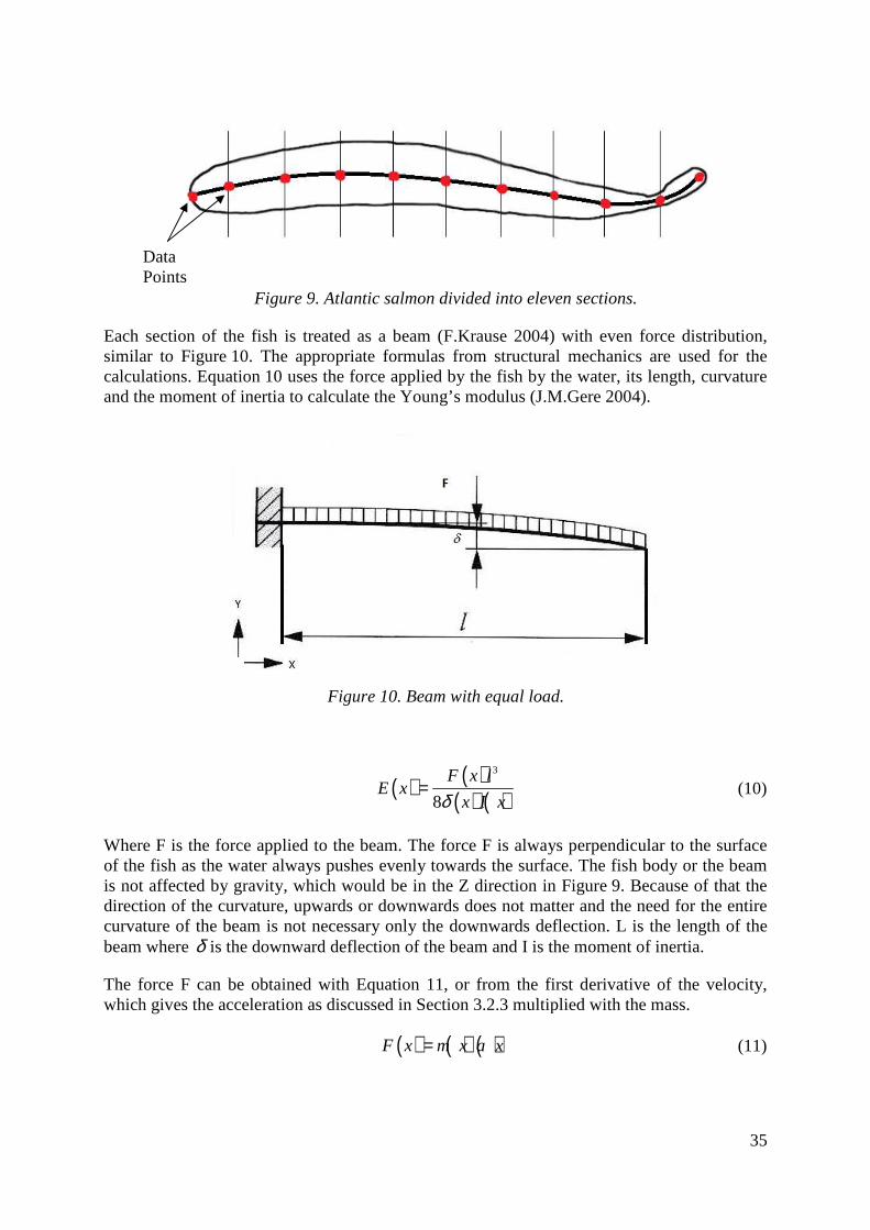
Figure 9

Each section of the fish is treated as similar to Figure 10. The appropriate formulas from structural mechanics calculations. Equation 10 uses the force appliedand the moment of inertia to calculate the

Where F is the force applied to the beam. The force F is always perpendicular to the surface of the fish as the water always pushes evenly towards the surface. The fish body or the beam is not affected by gravity, which would be in the Z direction in direction of the curvature, upwards or downwards does not mattercurvature of the beam is not necessary only the downwards deflection. Lbeam where δ is the downward deflection of the beam and I is the moment of inertia.

The force F can be obtained which gives the acceleration as discussed

Data Points

9. Atlantic salmon divided into eleven sections.

is treated as a beam (F.Krause 2004) with even force distributionhe appropriate formulas from structural mechanics

uses the force applied by the fish by the water, its length, curvature o calculate the Young’s modulus (J.M.Gere 2004)

Figure 10. Beam with equal load.

( ) ( )( ) ( )

3

8

F x lE x

x I xδ=

s the force applied to the beam. The force F is always perpendicular to the surface as the water always pushes evenly towards the surface. The fish body or the beam

, which would be in the Z direction in Figure 9. Because of that the direction of the curvature, upwards or downwards does not matter and the need for the entire curvature of the beam is not necessary only the downwards deflection. L

is the downward deflection of the beam and I is the moment of inertia.

d with Equation 11, or from the first derivative of the velocity, as discussed in Section 3.2.3 multiplied with the mass.

( ) ( ) ( )F x m x a x=

35

sections.

even force distribution, he appropriate formulas from structural mechanics are used for the

by the fish by the water, its length, curvature 2004).

(10)

s the force applied to the beam. The force F is always perpendicular to the surface as the water always pushes evenly towards the surface. The fish body or the beam

. Because of that the and the need for the entire

is the length of the is the downward deflection of the beam and I is the moment of inertia.

first derivative of the velocity, multiplied with the mass.

(11)

36

To calculate the moment of inertia the shape of the fish body must be taken into account. The shape can be approximated to a form of an ellipse as seen in figure 11. The real cross sectional area of a fish is very similar to an ellipse and can be seen in Figure 55 in the appendix.

Figure 11. Ellipse like cross-sectional area of the fish.

The moment of inertia for the cross-sectional area is given with Equation 12. Since the fish body bends around the y-axis, appropriate equation is used.

( ) ( ) ( ) ( )3

4y

b x a xI x I x

π= = (12)

To estimate the stiffness, moment of inertia and the Young’s modulus are used as displayed in Equation 13.

( ) ( ) ( )x E x I xκ = (13)

37

4 Experimental setup and procedure

This project uses the locomotion of Atlantic salmon to analyze and construct a mathematical model that describes the movements of the fish to determine the variables that change with different swimming velocities. The variables in question are amplitude, frequency, acceleration, phase difference and stiffness. The reason for choosing the Atlantic salmon and Arctic char was because of their availability in Iceland. Other types of fish are well suited for a study of this type. This chapter describes how the two experiments were set up and in what way they were conducted. The goal in experiment two is to transfer the oscillating motion of the fish to raw data for it to be processed through the numerical model. Experiment two aims to recreate the oscillating motion from the numerical model with a simple mechanical system.

4.1 Experiment in a swimming tunnel

To analyze the locomotion of fish one cannot simply observe the fish in its natural environment. To get valuable and accurate results the fish needs to be studied under controlled conditions. For controlling the conditions a small swimming tunnel designed specifically for testing the stamina of fishes was used. The tunnel, seen in Figure 12, allows for precise control of the water velocity and temperature while maintaining laminar flow conditions. The swimming tunnel, SW10050 is manufactured by Loligo systems and has a 5 liter capacity.

Figure 12. Loligo SW10050 Swim tunnel

For each test, a fish was placed in the swim tunnel and the water flow adjusted until steady flow conditions were obtained. The water temperature was maintained at 5.5°C. The minimum swimming speed was determined just above when the fish stopped swimming and lay on the bottom of the tank. The maximum swimming speed was determined when the fish could no longer sustain constant swimming and therefore going into burst swimming mode. The medium swimming mode is determined as the one between min and max.

The swimming tunnel was powered by a 370W electric motor and a speed controller. The frequency going into the motor was controlled allowing for increase and decrease in flow of the water from 3 – 110cm/s. The relationship between the frequency of the motor and the velocity of the water can be seen in Equation 14

38

0.0202 0.044V f= − (14)

As the frequency of the motor (variablef ) is increased the rpm of the water turbine increases and the flow increases.

The swimming was recorded by a JVC GY-HM100U video camera. Figure 13 shows a schematic of the camera setup. The camera was positioned 25.5 cm above the tank. The recording duration for each of the swimming modes was about one minute. From each recorded video a 1-2 second segment was extracted where the fish was stable and swam continuously. The extracted video segments were then analyzed.

Figure 13. Camera setup for experiment one. Camera placed above the swimming tunnel.

The camera, HD camera, was configured to HQ Mode. 1920 x 1080 60 frames per second which gave an acceptable resolution for determining and tracking the 11 data points on the back of the fish from head to caudal fin. A photo of the setup is shown in Figure 14.

Figure

Each frame was analyzed in Matlabthrough the x-y positions of the pointsbetween points. The nose of the fish was used as point zero to have a fixed point of reference. To accurately determine the center of every point on the fishradius of the distance to the pointwere laid on each side of the fish with a middle line connecting them. The intersection point between the circle and midpoint line gave the point for the center of the fish.Figure 15 demonstrates how a line is drawn between the lines and its center determines the location of the data point. An overlaid grid system then determines the coordinate and is logged down. A video recording system at 60 fps was used to record the movement of two fish species under different swimming conditions in a swimming tunnelvelocities were determined by the fishes where the minimum velocity was determined when the fish began to swim, the maximum when the fish gave up and the medium velocity in the middle.

Figure

Figure 14. Swimming tunnel, camera setup.

analyzed in Matlab and a second degree Fourier function was fitted y positions of the points. The length of the fish determined the distance

between points. The nose of the fish was used as point zero to have a fixed point of reference. To accurately determine the center of every point on the fishradius of the distance to the point was drawn. Two parallel lines perpendicular to the body

laid on each side of the fish with a middle line connecting them. The intersection point between the circle and midpoint line gave the point for the center of the fish.

w a line is drawn between the lines and its center determines the location of the data point. An overlaid grid system then determines the coordinate and is

A video recording system at 60 fps was used to record the movement of two under different swimming conditions in a swimming tunnel

velocities were determined by the fishes where the minimum velocity was determined when the fish began to swim, the maximum when the fish gave up and the medium

Figure 15. Method for determining the data points.

39

second degree Fourier function was fitted length of the fish determined the distance

between points. The nose of the fish was used as point zero to have a fixed point of reference. To accurately determine the center of every point on the fish, a circle with the

wo parallel lines perpendicular to the body laid on each side of the fish with a middle line connecting them. The intersection

point between the circle and midpoint line gave the point for the center of the fish. w a line is drawn between the lines and its center determines the

location of the data point. An overlaid grid system then determines the coordinate and is A video recording system at 60 fps was used to record the movement of two under different swimming conditions in a swimming tunnel. The three

velocities were determined by the fishes where the minimum velocity was determined when the fish began to swim, the maximum when the fish gave up and the medium

40

4.1.1 Arctic char

The Arctic char (Salvelinus alpinus) is a cold-water fish from the Salmonidae family, native to Arctic, sub-Arctic and alpine lakes and coastal waters. The Arctic char is quite common and a popular fish by fishermen in rivers and lakes where it can weigh up to 9 kg and “give a good fight”. It usually sits low near the bottom and fastens itself so it doesn’t have to swim and makes the river do the “swimming” for them and is therefore considered a bit of a lazy fish. However it can swim fast and sustain high speed swimming for long periods of time and can achieve up to 3 body length per second [Bl/s] in sustained swimming speed and up to 4 body lengths per second in burst mode. The char shown in Figure 16 was used in this experiment. It was 12.5 cm in length and weighed 23 grams.

Figure 16. Arctic Char in swimming tunnel.

4.1.2 Atlantic salmon

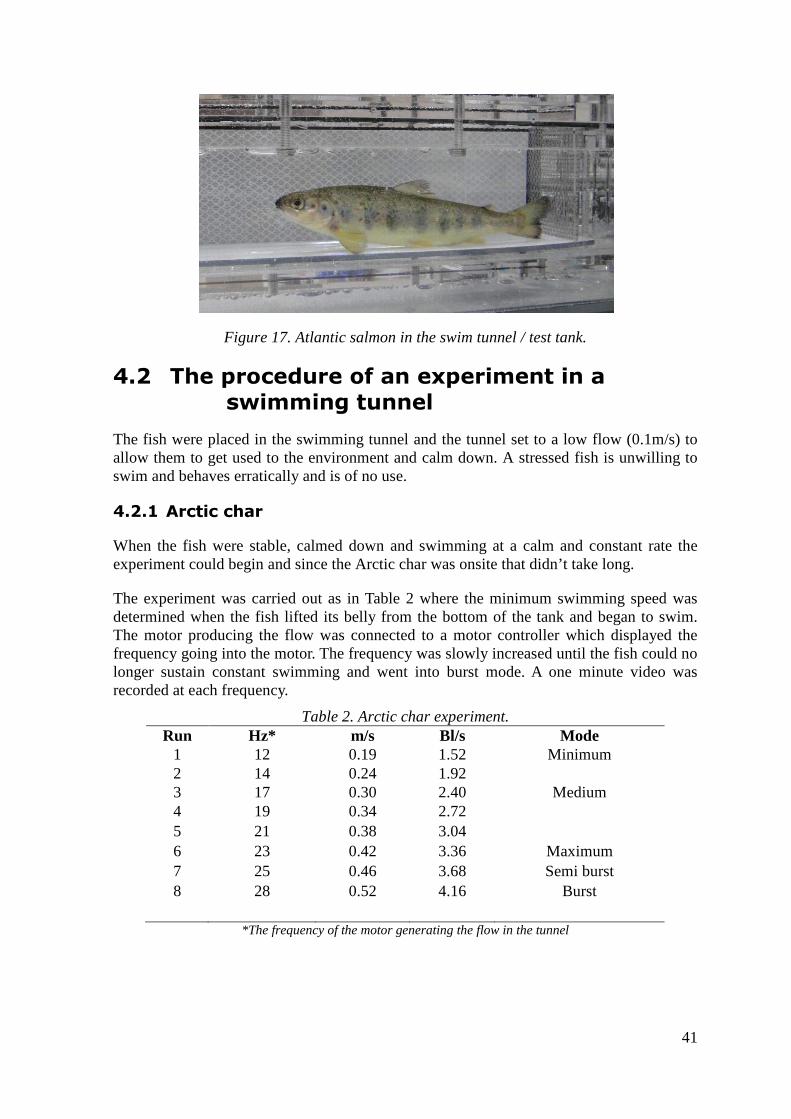
The Atlantic salmon comes from the Salmonidae family, which is found in the northern Atlantic Ocean and in rivers that flow into the north Atlantic. The salmon is considered more of a swimming fish (N.Bose 1992) than the Arctic char, in the sense that it swims more and faster. The salmon can achieve speeds up to five body lengths per second in constant swimming and well over seven body lengths in burst mode. The specimen shown in Figure 17 was used in the experiment. It was 15.2 cm long and weighed 48 grams.

41

Figure 17. Atlantic salmon in the swim tunnel / test tank.

4.2 The procedure of an experiment in a swimming tunnel

The fish were placed in the swimming tunnel and the tunnel set to a low flow (0.1m/s) to allow them to get used to the environment and calm down. A stressed fish is unwilling to swim and behaves erratically and is of no use.

4.2.1 Arctic char

When the fish were stable, calmed down and swimming at a calm and constant rate the experiment could begin and since the Arctic char was onsite that didn’t take long.

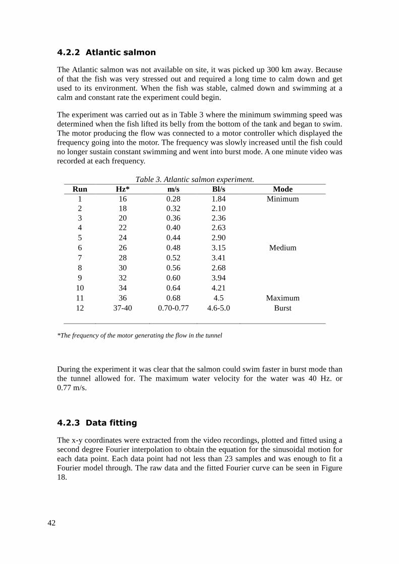
The experiment was carried out as in Table 2 where the minimum swimming speed was determined when the fish lifted its belly from the bottom of the tank and began to swim. The motor producing the flow was connected to a motor controller which displayed the frequency going into the motor. The frequency was slowly increased until the fish could no longer sustain constant swimming and went into burst mode. A one minute video was recorded at each frequency.

Table 2. Arctic char experiment. Run Hz* m/s Bl/s Mode

1 12 0.19 1.52 Minimum 2 14 0.24 1.92 3 17 0.30 2.40 Medium 4 19 0.34 2.72 5 21 0.38 3.04 6 23 0.42 3.36 Maximum 7 25 0.46 3.68 Semi burst 8 28 0.52 4.16 Burst

*The frequency of the motor generating the flow in the tunnel

42

4.2.2 Atlantic salmon

The Atlantic salmon was not available on site, it was picked up 300 km away. Because of that the fish was very stressed out and required a long time to calm down and get used to its environment. When the fish was stable, calmed down and swimming at a calm and constant rate the experiment could begin.

The experiment was carried out as in Table 3 where the minimum swimming speed was determined when the fish lifted its belly from the bottom of the tank and began to swim. The motor producing the flow was connected to a motor controller which displayed the frequency going into the motor. The frequency was slowly increased until the fish could no longer sustain constant swimming and went into burst mode. A one minute video was recorded at each frequency.

Table 3. Atlantic salmon experiment.

Run Hz* m/s Bl/s Mode 1 16 0.28 1.84 Minimum 2 18 0.32 2.10 3 20 0.36 2.36 4 22 0.40 2.63 5 24 0.44 2.90 6 26 0.48 3.15 Medium 7 28 0.52 3.41 8 30 0.56 2.68 9 32 0.60 3.94 10 34 0.64 4.21 11 36 0.68 4.5 Maximum 12 37-40 0.70-0.77 4.6-5.0 Burst

*The frequency of the motor generating the flow in the tunnel

During the experiment it was clear that the salmon could swim faster in burst mode than the tunnel allowed for. The maximum water velocity for the water was 40 Hz. or 0.77 m/s.

4.2.3 Data fitting

The x-y coordinates were extracted from the video recordings, plotted and fitted using a second degree Fourier interpolation to obtain the equation for the sinusoidal motion for each data point. Each data point had not less than 23 samples and was enough to fit a Fourier model through. The raw data and the fitted Fourier curve can be seen in Figure 18.

43

Figure 18. All data points plotted. Amplitude vs time from nose of the fish to its tail. Red circles represent the raw data points and the blue line the fitted Fourier model.

4.3 Measuring the volume of fish

The volume of the fish was measured and calculated with an optic measurement device provided by Marel inc. The fish was laid out on a moving conveyor belt that passed below the optic laser scanner. The optic laser scanned the surface of the fish, logging down the area that was interrupted by the laser. The scanning machine is a part of their fish processing line and is generally used to scan fish filets, calculate their volume for weighing and later processing. The results can be seen in Section 5.2.6

4.4 Recreation of the motion

In the second experiment the mathematical model derived in the first experiment was used. The purpose of the second experiment is to recreate the wave form of the Atlantic salmon with a prototype that is based on a mechanical solution.

There are numerous ways to recreate the oscillating motion of the fish. It is also important to recreate the motion in order to determine accuracy of the motion. The following setups were discussed and evaluated.

44

4.4.1 Hydraulic, electric or air powered jacks

One jack would be connected to each of the data points representing each point on the back of the fish (a total of eleven). A control module would then synchronize the motion, moving the fin up and down which would create thrust.

� Pros: The system could be easily adjusted to fine tune the motion and create maximum thrust at different velocities.

� Cons: The system would have to remain stationary because of weight. The water flow would have to be measured, which would increase inaccuracy because of difficulty to measure flow accurately. Each jack, hydraulic or other, is expensive. Overall complexity of the system would be high.

4.4.2 Design of a reciprocating crankshaft

A crankshaft made out of twelve individual disks connected together. Use the amplitude and phase difference to determine the locations for the holes on the discs which would connect each section of the shaft together. The drive would move in circles in a water filled tank.

� Pros: Mechanically simple. Inexpensive. Easy to measure the velocity of the assembly as it moves in circles

� Cons: Each crankshaft is fixed for a certain velocity field and cannot be adjusted. The weight of the assembly could be an issue which would result in more energy needed to move the assembly.

4.4.3 Servo motors

Use servo motors placed inside a fin like silicone-rubber based shell. The motors connected in a series where each joint represents a data point. The motors then controlled and programmed to move in sync and create an identical waveform to the motion of the fish.

� Pros: The motion can be adjusted constantly, similar to the hydraulic jack setup, with increased velocity.

� Cons: The system has limited velocity range due to the nature of servo motors which are not fast acting. The system is more expensive than the crankshaft solution and requires complex wiring and programming. The setup would also have to remain stationary and the water flow measured with its inaccuracy. The drive would also be submerged and water tight seals around electrical connections could become an issue.

4.4.4 Mechanical setup

To simulate the oscillating motion of the fish a mechanical solution needed to be implemented. There are numerous ways to reproduce oscillating motion. One way is to use hydraulic or air powered jacks to move up and down in synchronous motion. This requires addition electronic control units, each with their own power requirements which

45

increases parasitic losses and reduces the total efficiency of the system. In this project the fixed crankshaft method was chosen because of its simple construction and low budget.

Automobile engines also create oscillating motions where pistons move up and down. The pistons are connected together with a crankshaft. The crankshaft delivers the power to the transmission and eventually to the wheels. For a mechanical solution a type of crankshaft was built, one for each swimming velocity. Details on the crankshafts construction can be seen in appendix.

Three crankshafts were constructed, each for one swimming velocity, 1.84, 3.15 and 4.5 Bl/s. The crankshaft was connected via pins to the flexible foil which produced the thrust in the system and allowed to move in a circular motion in the tank. A 3D sketch of the crankshaft setup can be seen in Figure 19.

Figure 19. A 3D representation of the crankshaft used to recreate the oscillating motion of the fish.

The assembly rotates clockwise and is held in place by bearings at each end. The connection points for the pins between the discs are calculated form the phase difference with the correct amplitude.

4.4.5 Electronic motor controller and motor

The crankshaft was powered by a 90W electric motor. The motor was controlled with an electronic speed controller which allowed for control of the frequency in the system and adjust for the correct rotational speed of the crankshaft. The controller runs on 12VDC and can handle up to 50A. The controller can be seen in Figure 20.

Motor

Flexible rubber fin

46

Figure 20. Electronic speed controller for the motor.

The motor was a PM 759 12V-90W motor from a caravan air-condition unit. The motor had sufficient rpm range and power and suited well. The motor can be seen in Figure 21.

Figure 21. PM 759 12V-90W motor from a air conditioning unit. Used to control the rotational speed of the crankshaft and therefore its frequency.

4.4.6 The foil

The flexible foil is one of the most important items in the system. It transfers the energy from the oscillating motion in the crankshaft to the water in the tank and creates forward movement. The foil needs to be flexible to simulate the flexible motion of the fish. The foil was made from a 1mm thick rubber sheet. It’s strong enough to fasten the pins from the crankshaft to and flexible enough for the oscillating motion. The un-attached foil representing the fin can be seen in Figure 22.

47

Figure 22. The foil made out of 1mm rubber sheet.

To prevent side to side movement of the foil a 5mm acrylic sheets were placed on each side of the foil.

4.4.7 Water tank setup and mechanical frame

A steel frame was welded together to hold in place the crankshaft and to connect the motor to the shaft. The frame also held in place the acrylic sheets. The setup can be seen in Figure 23.

Figure 23. Steel frame construction. Side plates are made from Acrylic glass.

The frame was supported by magnets to create a magnetic levitation between the bars and the tank to eliminate friction and rolling resistance in wheels and minimize losses in the system. The magnet setup can be seen in Figure 24.

Motor controller

Motor

Crankshaft

Acrylic sheets

48

The magnets top magnets were N52 grade and capable of holding/repelling 100 kg each. The stationary tank magnets were N42 with a repellant force of 20 kg. The setup allowed the assembly to hover with 4cm clearance.

Figure 24. Magnetic levitation.

A 420 liter steel tank was constructed displayed in Figure 25. The experiment was only performed and based on the Atlantic salmon. This is because of the instability of the data for the Arctic char. The fluctuations in frequency and phase difference turned out to be too great for an accurate experiment and the effort better focused on Atlantic salmon.

Figure 25. 420L steel tank for the second experiment. Mechanical setup

A vertical steel pipe was placed in the middle of the tank. The pipe served as a bearing placement for a pair of horizontal bars. The bars hold in place the mechanical device to simulate the oscillating motion and electronic devices used in the experiment. The bars are separated by a about 30° angle and each bar has wheel on the end. The experimental setup can be seen in Figure 26.

Magnets

49

Figure 26. Experiental setup for the tank experiment. A steel frame supporting the rotating assembly connected to an electric motor. The crankshaft then delivers the oscillating motion to the flexible fin.

4.5 The execution of experiment two, the water tank

The tank was filled up with water and the motor was turned on and set to maximum rpm. It was immediately clear that the motor power was not enough. Because of that the assembly did not move fast enough to obtain one Bl/s. The assembly did move, but at a very slow rate for about 5-6 seconds and moved about 0,5 m. It was clear that this assembly would not perform as expected due to unforeseen problems, electronic and mechanical. Further improvements would be needed.

Vertical Pipe

50

51

5 Results

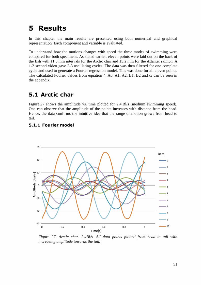
In this chapter the main results are presented using both numerical and graphical representation. Each component and variable is evaluated.

To understand how the motions changes with speed the three modes of swimming were compared for both specimens. As stated earlier, eleven points were laid out on the back of the fish with 11.5 mm intervals for the Arctic char and 15.2 mm for the Atlantic salmon. A 1-2 second video gave 2-3 oscillating cycles. The data was then filtered for one complete cycle and used to generate a Fourier regression model. This was done for all eleven points. The calculated Fourier values from equation 4, A0, A1, A2, B1, B2 and ꙍ can be seen in the appendix.

5.1 Arctic char

Figure 27 shows the amplitude vs. time plotted for 2.4 Bl/s (medium swimming speed). One can observe that the amplitude of the points increases with distance from the head. Hence, the data confirms the intuitive idea that the range of motion grows from head to tail.

5.1.1 Fourier model

Figure 27. Arctic char. 2.4Bl/s. All data points plotted from head to tail with increasing amplitude towards the tail.

-60

-40

-20

0

20

40

60

0 0,2 0,4 0,6 0,8 1

Am

pli

tud

e[p

ixe

ls]

Time[s]

0

1

2

3

4

5

6

7

8

9

10

Data

52

In order to see the difference more clearly it is better to look at the data for selected points 2.4 Bl/s is plotted in Figure 28. All parameters for the Fourier series can be found in the appendix.

Figure 28. Arctic char 2.4 Bl/s. Data points 0, 1, 6 and 10 at same frequency and increased amplitude.

Here one can observe that the wavelength λ does not change much towards the tail. The frequency should stay the same at constant speed but as you can see the frequency fluctuates a little bit and is considered to be data error. Generally the amplitude should increase.

21 3A A A< < (15)

And in this case it does, however points zero and one does not fit to this hypothesis, this is because the center of mass (G.V.Lauder 2006) for fishes lies between 1 4 and 1 3 of their body length (point 2 in this case), so that the oscillating motion increases after the center of mass towards the nose. In this case Equation 15 becomes

30 1 2 4 5 10......> > A A A A AA A < < < (16)

This is an important feature which is often overlooked and possibly contributes to thrust generation especially at higher speeds as it pumps higher velocity water to the rest of the body. To see how the motion of the fish changes with increased speed a comparison

-80

-60

-40

-20

0

20

40

60

80

0 0,2 0,4 0,6 0,8 1

Am

pli

tud

e[p

ixe

ls]

Time[s]

0

1

6

10

Data

Points

53

of the same point on the back of the fish (data point 8) is displayed in Figure 29 over the three different velocities. 1.5 Bl/s. 2.4 Bl/s and 3.36 Bl/s.

Figure 29. Arctic char. Data point 8 for 1.5. 2.4 and 3.36 Bl/s. With standard error.

It is also interesting to see how much the amplitude changes at the caudal fin and near it in Figure 30, about 28%.

-50

-40

-30

-20

-10

0

10

20

30

40

50

0 0,2 0,4 0,6 0,8 1

x-c

oo

rdin

ate

s

Time[s]

1,5Bl/s

2,4Bl/s

3,36Bl/s

54

Figure 30. Amplitude of Data points 9 and 10. With standard error.

The data in Table 4 shows that when the swimming speed of the fish increases the frequency increases.

Table 4. Frequency change with increased speed. Velocity [Bl/s] Frequency [Hz]

1.52 1.97 2.4 2.21 3.36 1.73

A 37% increase in velocity results in a 10% increase in frequency. But the frequency drops at 3.36 Bl/s. this might be due to data error and unsteady swimming in the fish, but a nominal 10% increase was general.

In the Arctic char the frequency fluctuation was more than expected at lower swimming speed but it kept at a constant rate for higher speed. When looked at Table 5, one can see that the amplitude also increases as the fish swims faster. This is depicted graphically in Figure 31.

-100

-80

-60

-40

-20

0

20

40

60

80

100

0 0,2 0,4 0,6 0,8 1 1,2 1,4 1,6

Am

pli

tud

e[p

ixe

ls]

Time[s]

9

10

Data

Points

55

Table 5. Amplitude change during swimming. Bl/sec Average

Amplitude [cm] %

increase 1.52 0.58 0 2.4 0.7 17 3.36 0.79 11

The amplitude increases with increased speed can be seen in Figure 31. Excluding point two where the center of mass is we see an amplitude drop. The Arctic char has maximum amplitude of 1.5 cm. or corresponding to its length, about 12%. The percent increase in amplitude also drops as the swimming speed becomes higher.

Figure 31. Amplitude change. All data points. Arctic char. With standard error.

Phase difference and the change in flexibility calculations were not done for the Arctic char because of insufficient resolution in the data causing high fluctuation with increased data error.

5.2 Atlantic salmon

5.2.1 Fourier model

A Fourier model for every other data point is plotted in Figure 32. The plot corresponds to the results in the Arctic char. where the frequency should remain relatively stable length wise and the amplitude rise the further down the fish.

-0,2

0

0,2

0,4

0,6

0,8

1

1,2

1,4

1,6

1,8

2

0 2 4 6 8 10 12

Am

pli

tud

e [

cm]

Data Points

1,54

2,5

3,36

Bl/s

56

Figure 32. Every other data points at 3.15 Bl/s. Atlantic salmon.

Similar to the Arctic char and all other fish the amplitude increases towards the tail. Point zero, or the nose of the fish, also has higher amplitude than point 2 because of the center of mass.

5.2.2 Frequency

The frequency changes as seen in Figure 33 with different velocity, but should stay relatively constant over the fish body at constant speed.

Figure 33. Frequency plot. Atlantic Salmon. With 6%. 4% and 8% std error.

-60

-40

-20

0

20

40

60

0 0,2 0,4 0,6 0,8 1

Am

pli

tud

e[p

ixe

ls]

Time[s]

0

2

4

6

8

10

Data

Points

1

1,5

2

2,5

3

3,5

0 2 4 6 8 10

Fre

qu

en

cy [

hz]

Data Point

Bl/s

1,84

3,15

4,5

57

The frequency as displayed in Figure 33 fluctuates; it has a maximum fluctuation of about 30% at 4.5 Bl/s. mainly close to the center of mass at point two where the error margin is highest. Notice how the frequency is slightly lower from the nose of the fish till the center of mass. This implies different behavior of the nose and its possible contribution to thrust generation where it accelerates the incoming flow to the rest of the body.

Table 6. Frequency change during swimming.

Bl/sec Average Hz % increase 1.84 1.6 0 3.15 2.1 32 4.5 2.9 36

Table 6 gives that for each increase in body length the average frequency increases of about 21%. The frequency also seems to be a lot more stable in the Atlantic salmon than the Arctic char. The frequency increase is a linear one. The relationship is displayed in Figure 34.

Figure 34. Linear frequency increase as a function of body length velocity with standard error.

5.2.3 Acceleration

The acceleration is calculated using Equation 7 for data points 4-10 in Figure 35.

y = 0,4768x + 0,6789

0

0,5

1

1,5

2

2,5

3

3,5

0 1 2 3 4 5

Fre

qu

en

cy[h

z]

Body length per second [Bl/s]

Linear

(Frequency)

58

Figure 35. Acceleration for Atlantic salmon. Data points 4-10. 1.84, 3,15 and 4.5 Bl/s

The point acceleration increases as the fish swims faster. The increase between swimming velocities is not linear as displayed in Figure 36. The acceleration at data point 8 at 4,5 Bl/s has a sudden increase. This is thought to be data error as its correlates with a slight amplitude increase in Figure 37.

Figure 36. Non linear interaction between data points with increased swimming velocity. Data points 4,6,8 and 10.

The average increase from 1,84 Bl/s to 3,15 Bl/s was 47% and the increase from 3,15 Bl/s to 4,5 Bl/s was 60%

0

2

4

6

8

10

12

3 4 5 6 7 8 9 10 11

Acc

ele

rati

on

[m

/s2

]

Data Point

1,84

3,15

4,5

Bl/s

0

1

2

3

4

5

6

7

8

9

10

0,75 1,25 1,75 2,25 2,75 3,25

Acc

ele

rati

on

[m

/s2

]

Body length per second[Bl/s]

Data

Point

4

6

8

10

59

5.2.4 Amplitude

The amplitude plot, shown in Figure 37, is similar to that of the Arctic char, but it seems to have higher amplitude at the tip of the nose than the Arctic char. The amplitude increases the faster the fish swims. Figure 37 displays data points 4-10. The errors around the center of mass are at its highest and points 0-4 are not necessary for the tank experiment, so they are not displayed in Figure 37.

Figure 37. Atlantic salmon amplitude change over 1,84. 3,15 and 4,5 Bl/s

A polynomial line was plotted through the data points, using excel, to obtain an equation for the data. The polynomial plot can be seen in Figure 38 and the equations in Table 7.

Figure 38. Polynominal plot for amplitude data. Data points 4-10.

0

0,2

0,4

0,6

0,8

1

1,2

1,4

1,6

1,8

2

3 4 5 6 7 8 9 10 11

Am

pli

tud

e [

cm]

Data Points

Bl/s

1,84

3,15

4,5

0

0,2

0,4

0,6

0,8

1

1,2

1,4

1,6

1,8

3 4 5 6 7 8 9 10 11

Am

pli

tud

e [

cm]

Data Points

Bl/s

Poly.

(1,84)

Poly.

(3,15)

Poly. (4,5)

60

The polynomial fit correlates well to the data points, with a minimum of 98,8% correlation.

Table 7. Atlantic salmon polynominal equations. Velocity Equation Correlation 1.84Bl/s 20.0218 0.2789 0.8208x x− + 98.9% 3.15Bl/s 20.0293 0.2715 0.887x x− + 99.9% 4.5Bl/s 20.0355 0.2789 0.8208x x− + 99.5%

The amplitude increases with increased swimming speed as well as increases the closer you get to the caudal fin. In Table 8 one can see how the average amplitude increases between different speeds.

Table 8. Amplitude change in Atlantic salmon.

Bl/sec Average A [cm] % increase 1.84 0.35 0 3.15 0.41 15 4.5 0.59 30

When reaching higher speeds the amplitude doubles where the average difference between 3.15 Bl/s and 4.5 Bl/s is about 30% where it is about 15% between 1,84 and 3,15 Bl/s. As body length velocity increased the curvature becomes linear and has an average increase of 20-25% per increased body length velocity above 3 Bl/s. The curvature increase can be seen in Figure 39.

Figure 39. Amplitude increase vs Body length per second with standard error. Atlantic salmon.

There seems to be more increase in amplitude in the Atlantic salmon than the Arctic char when changing from low speed swimming to high. The Atlantic salmon has maximum

0

0,2

0,4

0,6

0,8

1

1,2

1,4

1,6

1,8

2

1 1,5 2 2,5 3 3,5 4 4,5 5

Am

pli

tud

e[c

m]

Body length per second[Bl/s]

10

8

6

4

Data

Points

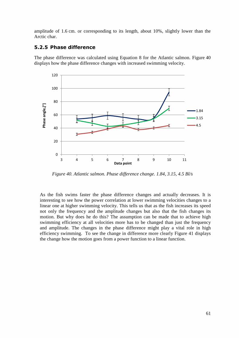
61

amplitude of 1.6 cm. or corresponding to its length, about 10%, slightly lower than the Arctic char.

5.2.5 Phase difference

The phase difference was calculated using Equation 8 for the Atlantic salmon. Figure 40 displays how the phase difference changes with increased swimming velocity.

Figure 40. Atlantic salmon. Phase difference change. 1.84, 3.15, 4.5 Bl/s

As the fish swims faster the phase difference changes and actually decreases. It is interesting to see how the power correlation at lower swimming velocities changes to a linear one at higher swimming velocity. This tells us that as the fish increases its speed not only the frequency and the amplitude changes but also that the fish changes its motion. But why does he do this? The assumption can be made that to achieve high swimming efficiency at all velocities more has to be changed than just the frequency and amplitude. The changes in the phase difference might play a vital role in high efficiency swimming. To see the change in difference more clearly Figure 41 displays the change how the motion goes from a power function to a linear function.

0

20

40

60

80

100

120

3 4 5 6 7 8 9 10 11

Ph

ase

an

gle

,[°]

Data point

1.84

3.15

4.5

62

Figure 41. Atlantic salmon. Polynomial to linear change with increased swimming velocity.

The decrease in phase difference can be seen in Table 9.

Table 9. Phase difference change in Atlantic salmon. Bl/sec Phase difference

[°] % decrease

1.84 61 0 3.15 51 15 4.5 38 24

5.2.6 Volume

The results from the optic scan can be seen in Figure 42

R² = 0,6538

R² = 0,9786

R² = 0,6915

28

38

48

58

68

78

88

3 4 5 6 7 8 9 10 11

Ph

ase

an

gle

,[°]

Data Points

Bl/s

1.84

3.15

4.5

63

Figure 42. Measured area of Atlantic salmon.

As expected the cross sectional area of the fish increases up to about the 50 mm point and then decreases towards the tail of the fish. Numerical results can be seen in Table 10.

Table 10. Volume measurement results. Position Area[mm2] Volume[ml]

0 0 0.00 8.25 190 1.57

16.50 345 2.85 24.75 450 3.71 33.00 542 4.47 41.25 620 5.12 49.50 673 5.55 57.75 670 5.53 66.00 655 5.40 74.25 630 5.20 82.50 592 4.88 90.75 530 4.37 99.00 470 3.88

107.25 410 3.38 115.50 360 2.97 123.75 270 2.23 132.00 200 1.65 140.25 110 0.91 148.50 100 0.83 156.75 0 0.00

Total 7817 64.49

The total volume of the Atlantic salmon was 64.5 ml. To calculate the density equation 9 is used and the previously measured volume. Variables a and b from Figure 11 were calculated

0

100

200

300

400

500

600

700

800

0 50 100 150

Are

a[m

m2

]

Length[mm]

Atlantic

Salmon

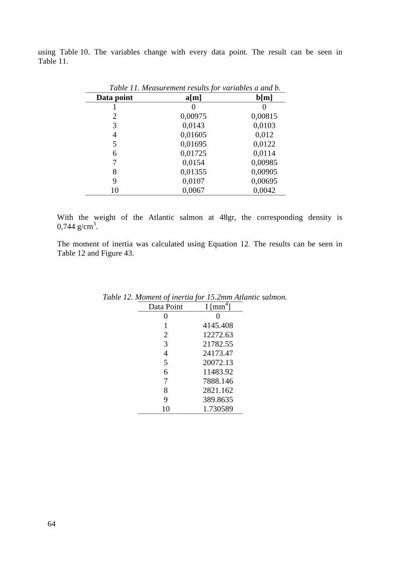
64

using Table 10. The variables change with every data point. The result can be seen in Table 11.

Table 11. Measurement results for variables a and b.

Data point a[m] b[m] 1 0 0 2 0,00975 0,00815 3 0,0143 0,0103 4 0,01605 0,012 5 0,01695 0,0122 6 0,01725 0,0114 7 0,0154 0,00985 8 0,01355 0,00905 9 0,0107 0,00695 10 0,0067 0,0042

With the weight of the Atlantic salmon at 48gr, the corresponding density is 0,744 g/cm3.

The moment of inertia was calculated using Equation 12. The results can be seen in Table 12 and Figure 43.

Table 12. Moment of inertia for 15.2mm Atlantic salmon.

Data Point I [mm4] 0 0 1 4145.408 2 12272.63 3 21782.55 4 24173.47 5 20072.13 6 11483.92 7 7888.146 8 2821.162 9 389.8635 10 1.730589

65

Figure 43. Moment of inertia distribution. Atlantic salmon.

Similar to the area distribution from Marel’s laser scanner the moment of inertia increases towards point 4, then decreases towards the tail. Last data point, number 10 has very low inertia. That is due to the shape of the tail fin, which at that point is more like a line than an ellipse.

5.2.7 Flexibility

As stated earlier to calculate the change in stiffness the Young’s modulus, moment of inertia, force and volume had to be calculated.

Results for the Young’s modulus can be seen in Figure 44.

Figure 44. Change in Young’s modulus for Atlantic salmon.

The increase in the Youngs’s modulus appears to be non-linear. The difference can be seen more clearly in Figure 45.

0

5000

10000

15000

20000

25000

30000

0 2 4 6 8 10

Mo

me

nt

of

Ine

rtia

[m

m4

]

Data Points

I[mm4]

0

200

400

600

800

1000

1200

1400

1600

3,5 4,5 5,5 6,5 7,5 8,5

Yo

un

g's

Mo

du

lus

[Pa

]

Data points

Bl/s

4.5

1.84

3.15

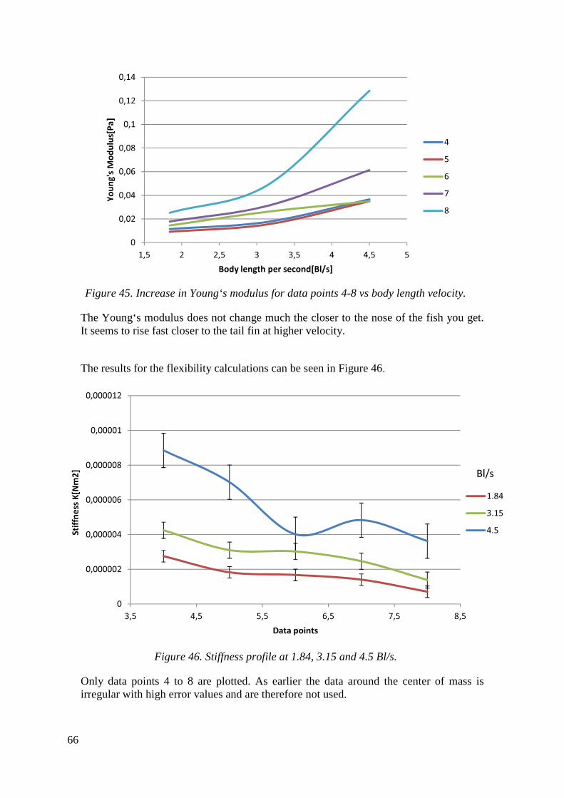
66

Figure 45. Increase in Young‘s modulus for data points 4-8 vs body length velocity.

The Young‘s modulus does not change much the closer to the nose of the fish you get. It seems to rise fast closer to the tail fin at higher velocity.

The results for the flexibility calculations can be seen in Figure 46.

Figure 46. Stiffness profile at 1.84, 3.15 and 4.5 Bl/s.

Only data points 4 to 8 are plotted. As earlier the data around the center of mass is irregular with high error values and are therefore not used.

0

0,02

0,04

0,06

0,08

0,1

0,12

0,14

1,5 2 2,5 3 3,5 4 4,5 5

Yo

un

g's

Mo

du

lus[

Pa

]

Body length per second[Bl/s]

4

5

6

7

8

0

0,000002

0,000004

0,000006

0,000008

0,00001

0,000012

3,5 4,5 5,5 6,5 7,5 8,5

Sti

ffn

ess

K[N

m2

]

Data points

Bl/s

1.84

3.15

4.5

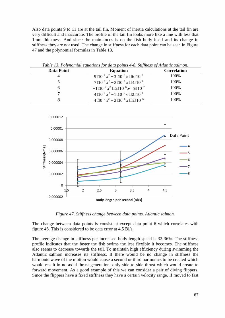
67

Also data points 9 to 11 are at the tail fin. Moment of inertia calculations at the tail fin are very difficult and inaccurate. The profile of the tail fin looks more like a line with less that 1mm thickness. And since the main focus is on the fish body itself and its change in stiffness they are not used. The change in stiffness for each data point can be seen in Figure 47 and the polynomial formulas in Table 13.

Table 13. Polynomial equations for data points 4-8. Stiffness of Atlantic salmon. Data Point Equation Correlation

4 7 2 6 69 10 3 10 6 10x x− − −⋅ − ⋅ + ⋅ 100% 5 7 2 6 67 10 3 10 4 10x x− − −⋅ − ⋅ + ⋅ 100% 6 7 2 6 71 10 2 10 9 10x x− − −− ⋅ + ⋅ − ⋅ 100% 7 7 2 6 64 10 1 10 2 10x x− − −⋅ − ⋅ + ⋅ 100%

8 7 2 6 64 10 2 10 2 10x x− − −⋅ − ⋅ + ⋅ 100%

Figure 47. Stiffness change between data points. Atlantic salmon.

The change between data points is consistent except data point 6 which correlates with figure 46. This is considered to be data error at 4,5 Bl/s.

The average change in stiffness per increased body length speed is 32-36%. The stiffness profile indicates that the faster the fish swims the less flexible it becomes. The stiffness also seems to decrease towards the tail. To maintain high efficiency during swimming the Atlantic salmon increases its stiffness. If there would be no change in stiffness the harmonic wave of the motion would cause a second or third harmonics to be created which would result in no axial thrust generation, only side to side thrust which would create to forward movement. As a good example of this we can consider a pair of diving flippers. Since the flippers have a fixed stiffness they have a certain velocity range. If moved to fast

-0,000002

0

0,000002

0,000004

0,000006

0,000008

0,00001

0,000012

1,5 2 2,5 3 3,5 4 4,5

Sti

ffn

ess

[Nm

2]

Body length per second [Bl/s]

Data Point

4

5

6

7

8

68

the flippers start to bend and form a second or third harmonics and produce little or no thrust.

5.3 Comparison of Arctic char and Atlantic salmon

Although related the Arctic char and the Atlantic salmon differ in how they swim. The Atlantic salmon has a larger range and can swim faster. The comparison will only be done for the frequency and amplitude. This is because of high fluctuation in the data for the Arctic char which lead to large errors in for example the phase difference which lead to incomparable results.

5.3.1 Frequency

As mentioned earlier although highly related both the frequency range and behavior differs significantly. The Atlantic salmon has much longer frequency range, starts lower and finishes higher and the frequency curve is almost linear increasing as the fish swims faster. The Arctic char however has a higher starting frequency than the Atlantic salmon but has a much shorter frequency range. It also does not seem to fallow the same linear increment of the salmon but fallows a type of parabolic curve where it has a maximum frequency at its medium swimming velocity and decreases the faster it goes after that. The result can be seen in Figure 48.

Figure 48. Frequency increase vs body length speed comparason for Arctic char and Atlantic salmon. Average values.

It is unclear if the decrease in the frequency is because of data error in the Arctic char or this is normal behavior.

1

1,5

2

2,5

3

1 2 3 4 5

Hz

Body Length per second [Bl/s]

Arctic

Char

Atlantic

salmon

69

5.3.2 Amplitude

The amplitude also differs significantly. The Arctic char has higher amplitude on all velocities. It also has an almost linear increase with increased body length speed. The Atlantic salmon has lower amplitude on almost all velocity ranges compared to the Arctic char. It also follows an upwards curve increasing more as it swims faster. The comparison can be seen in Figure 49.

Figure 49. Amplitude vs body length speed comparason for Arctic char and Atlantic salmon. Average values.

5.4 Tank experiment and mechanical assembly

The assembly was turned on and started moving at a slow pace. The assembly moved about half a meter. Then the powerful top magnets latched on to the tank itself and snapped down, bypassing the narrower tank magnets. The impact caused the whole electronic assembly to come loose and fell into the tank destroying the electronic speed controller and damaging the battery and motor.

In theory tank experiment was a simple way to recreate the oscillating motion of the Atlantic salmon, but from the beginning was plagued with unforeseen practical problems. For example to measure water velocity requires expensive measuring equipment and has an issue with accuracy. The solution was to allow the flexible drive to travel in circles and measure the velocity of the assembly itself. Simple enough, but turned out to have problems of its own.

From a visual observation the assembly did move about half a meter in about 5-6 seconds. Which results in 0,1 m/s or 0,16 Bl/s since the fin was 60 cm long. But no data can be represented to verify the result. Nor could the thrust be measured that the fin produced which eliminated any efficiency calculations.

0,2

0,3

0,4

0,5

0,6

0,7

0,8

0,9

1 2 3 4 5

Am

pli

tud

e[c

m]

Body Length per second [Bl/s]

Arctic

Char

Atlantic

salmon

70

To recreate the experiment the following is proposed:

• A fully submerged fin is held stationary and the flow measured

• A more rigid and stable crankshaft assembly constructed and balanced

• Only the back part of the fish used for thrust generation (data points 4-10) o The first half of the fish (data points 0-3) have very small amplitude and

their thrust generating part limited.

• A more power full motor with a wide rpm range

The alterations could result in an experiment where the efficiency of the motion can be measured and used to fine tune the numerical results.

71

6 Discussion

This chapter uses the numerical results and experiments and theorizes how they could be implemented to design and build flexible fin drive that could be utilized for propulsion in marine vessels.

6.1 Designing a flexible fin for a fishing vessel

The numerical results from experiment one can now be used theoretically to construct a flexible fin propulsion system.

As discussed in Chapter 4.4 there are numerous ways to recreate the oscillating motion of fish. For the most practical one let’s consider a single intake power fin where the force applied to the fin comes from one point transferred for an example via shaft. Fewer components and simplicity increases life and decreases the likelihood of component failure. A simple drawing is displayed in Figure 50.

Figure 50. Single input flexible fin.

The fin itself is constructed out of a uniform material and its thickness calculated to simulate the change in flexibility length wise which would result in a fin drive that is optimum at a certain velocity with a fixed flexibility velocity vise. The fin could be well suited for small fishing vessels where the speed of the boats is set at a level where the engine and the marine propeller are most efficient to minimize oil consumption. The material for the fin would be selected for a certain velocity range which would suit the vessel.

6.1.1 The vessel

In this case let’s consider a typical small fishing vessel with an average weight of 3500-5000 kg. The boat typically sails at about 6-18 knots to a fishing area. The propeller of the boat has a swept area of about 900cm2. To compare the fin and the propeller on the same basis the maximum swept area will be the same for the fin. Calculations are based on 10 knots, or about 5m/s and 900 cm2 swept area.

6.1.2 Fin material

To create a fin that has the behavior of a fish, the appropriate material has to be chosen. One with similar density and flexibility. In this case KE-941-U, a silicone rubber compound was chosen.

Input force Flow

Flow direction

72

Its density is slightly higher, or 1,3 gr/cm3, versus 0,744 gr/cm3 for the fish. To theoretically create a fin, data points 4-8 are used. Below data point 4 is little movement in amplitude so thrust generation is limited, also that part of the fish body mainly acts as a “storage space” for the internal organs. Data points 9 and 10 are the thin fin itself and calculations there have a very high error so they are not used.

6.1.3 Fin thickness calculations

To calculate the correct variables a new density is entered into the model were Equations 9-13 are used. New Young’s modulus and stiffness are recalculated using the different density of the silicone-rubber compound. The rest of the variables such as moment of Inertia, volume, amplitude and width of the fin are scaled up linearly. The equations are then solved for b, or the thickness at each point. See Equation 17.

33

32 Ib

Fl

κδ= (17)

The resulting thickness varies with length and becomes less towards the tail, much like the fish itself. The results can be seen in Table 14.

Table 14. Theoretical fin for a fishing boat cruising at 10knots(5,1m/s). Data Point 2b [cm]

4 13,5 5 11,7 6 9,9 7 6,9 8 4,1

The fin is 30cm wide and 74cm long. It has a maximum thickness of 13,5cm. The maximum amplitude is 11,3cm, which results in a top to bottom amplitude of 22,5cm at the tail. A graphical representation can be seen in Figure 51.

Figure 51. Artificial fin for small fishing vessel.

The fin could be used to propel a small fishing boat to about 10knots and would be at peak efficiency at that sailing speed. It would function well below that speed, but would

73

soon produce less thrust at higher velocity. This effect is similar to the diving flippers effect where second and third harmonics would be created producing more perpendicular thrust than axial.

6.2 Variable fin drive

The fin drive has a fixed flexibility and is therefore only suited for a specific velocity range and has a maximum swimming velocity. To actively maintain high propulsion efficiency the flexibility of the fin has to be controlled in relations with velocity. But to do this requires innovative and a practical solution that can last and outlast the conventional marine propeller. The following ideas surfaced during the project.

6.2.1 Linearly activated jacks

The connection points are linked to the fin and controlled precisely. This allows for accurate control of the flexible fin itself. The jacks move up and down in sync to produce thrust through a flexible foil.

� Pros: Accurate and easily controllable � Cons: Lifetime could be a problem since linear jacks, hydraulic, electronic or

other have a limited number of cycles and in a fast acting system with numerous movements per second lifetime is reduced.

6.2.2 Variable stiffness material (The ideal material)

The flexible fin would be made out of a material, similar to non-Newtonian fluid. The material increases its stiffness with increased load and therefore maintaining appropriate stiffness on all velocity ranges. Such a material does not exist but a similar material could be experimented with, such as D3O. D3O could not be obtained from the manufacturer due to low quantity and the nonexistent willingness to work with universities. The fin would be connected to a single force input, similar to Figure 50 and the rest of the fin is designed to react appropriately.

� Pros: Considerably the best solution, energy and lifetime wise. � Cons: The material does not exist.

6.2.3 Variable stiffness using ferro fluid and magnetic fields.

The fin would have an outer shell made out of a silicone-rubber compound. The inner layers divided into pockets. Each pocket would be filled up with ferro fluid. Above and below the fin large controllable magnets would be placed and the magnetic field adjusted until the desired stiffness reached.

� Pros: Simple and existing materials can be used. With high life expectancy � Cons: To generate the magnetic field requires energy which lowers the whole

efficiency of the system. The ferro fluid is not considered to be environmentally friendly and could contaminate the ocean in case of leakage.

74

6.2.4 Variable stiffness using water injection.

Similar to the ferro fluid fin, pockets are placed inside the flexible fin in a specific order and thicknesses. Sea water is then pumped into the drive as the vessel increases its speed which should increase the stiffness of the fin, inflating it in a way.

� Pros: Simple to try and could last a long time. No hazard in case of leakage. � Cons: Requires a pump to inflate the fin and a cleaver solution has to be found how

to pump in the fluid without disturbing the oscillating motion while maintaining a secure and lasting connection of the pipe to the fin. The inflation procedure could distort the shape of the fin itself and increase drag.

6.2.5 Variable stiffness using electronically active metals.

A type of electronically controlled metal strips that change their shape when electric current is applied could be used. The strips would be placed longitudinally with a certain cap between them. When voltage is applied, the strips try to retain a certain form thereby creating resistance against the movement of the fin and increasing its stiffness.

� Pros: Simple construction only needs an electronic connection. � Cons: Only one setting, either off or on, so the fin could only be efficient on two

velocity ranges, with the electronics off or on. Fatigue could also become an issue in the metals after so many cycles.

The use of electronic devices such as PWM (pulse width modulation) is also a possibility to control the electronic signal but it requires further study and implementation.

It is clear that there are numerous ways to recreate oscillating motion some better suited that others. It is this author’s opinion that the most efficient and practical solution would be to develop a non-Newtonian material that would react appropriately to increased force.

75

7 Conclusion

This study addresses the variables needed to construct a variable stiffness artificial flexible fish like fin to mimic that of Atlantic salmon. However, uniform adaptive materials to build a variable stiffness flexible fin are currently not available. That doesn’t mean it can’t be done. A few ideas came up during the project, such as using ferro fluid filled compartments and magnetic fields to try to change the resistance of the fluid and thereby changing the stiffness. Other idea was to use pressurized air or fluid and pump it into sections of the fin to, again, change the stiffness. For the time being the only practical solution is to design a flexible fin that is most efficient on a certain velocity. Since most boats cruise on a velocity optimized for the engine and the hull configuration. Majority of the time they cruise at a constant speed and vary only when docking or in heavy seas. With that in mind a flexible fin could be designed for any boats specific velocity range, where boat, engine and fin are at their optimum.

When comparing the Arctic char and the Atlantic salmon, although related, their swimming performance, mode and behavior differs. The salmon can swim faster, increases its amplitude more between swimming modes and has more stable frequency at constant swimming speed but has a lower amplitude compare to the Arctic char.

For the Atlantic salmon the frequency changes about 10-18% percent per increased body length speed. The amplitude changes about 25% for every increased body length speed.

Phase difference behavior gives an image how the fish behaves under different swimming velocities. The phase difference decreases an average of 15% from 1,84 Bl/s to 3,14 Bl/s and 25% from 3,15 Bl/s to 4,5 Bl/s. The change is also not linear and the curves go from being polynomial functions to linear functions at the maximum swimming velocity. The phase difference calculations alone give an interesting result, they show that the swimming behavior differs significantly and changes during swimming. This gives a good indication that the locomotion of fish is more complex and many factors govern their locomotion than simply frequency and amplitude.

The main goal of this project was to demonstrate and prove the assumption that the stiffness of swimming fish or how it increases with increased swimming velocity. To calculate the change in stiffness, the curvature of the fish was treated as a beam and the Young’s modulus calculated as for the moment of inertia. The mass properties and the acceleration were also calculated which allowed for the stiffness to be obtained. It has now been demonstrated that there is an average stiffness change of 32-36% per body length speed and cannot be considered as completely linear.

The results of this thesis can be used to design a flexible fin propulsion system for marine applications suited for a specific velocity range to obtain high efficiency. This could lead to lower energy requirements in marine propulsion which would reduce greenhouse gas emissions from marine vessels.

77

References

C. D. Wilga, G. V. Lauder. 2004. Hydrodynamic Function of the Shark’s Tail. Nature, vol. 430, no. 7002, pp. 850. C.M. Breder. 1926. locomotion of fishes in, Journal of experimental biology.

D.A. Read. F.S. Hover. M.S. Triantafyllou. 2002 “Forces on oscillating foils for propulsion and maneuvering” Dept of Ocean engineering MIT USA.

Douglas C. Montgomery and George C. Runger. 2005 “Applied Statistics and Probability for Engineers” Fourth Edition.

E. D. Tytell, G. V. Lauder. 2004. The Hydrodynamics of Eel Swimming I. Wake Structure. Journal of Experimental Biology, vol. 207, no. 11, pp. 1825−1841. Erik J. Anderson, Wader. McGillis, Mark A. Grosenbaugh. 2000.The boundary layer of swimming fish. Department of Applied Ocean Physics and Engineering, Woods Hole Oceanographic Institution, Woods Hole. MA, USA. December 2000.

Falk, Krause, Tiedt. 2004 “Töflubókin – Fyrir málm- og véltækni” 7th edition.

Frank.E Fish, 1992. Power output and propulsive efficiency of swimming Bottlenose dolphins. Journal of experimental biology. 185, 1993

Georg V Lauder and Peter G.A Madden 2006 “Learning from fish: Kinematics and experimental Hydrodynamics for Robotics” Harvard University Cambridge USA.

G. V. Lauder. Locomotion, 2006 The Physiology of Fishes, 3rd ed., D. H. Evans, J. B. Claiborne, Eds., CRC Press, Boca Raton, pp. 3−46,. G. V. Lauder, E. G. Drucker, J. Nauen, C. D. Wilga. 2003. Experimental Hydrodynamics and Evolution: Caudal Fin Locomotion in Fishes. Vertebrate Biomechanics and Evolution, V.Bels, J.-P. Gasc, A. Casinos, Eds., Bios Scientific Publishers, Oxford, pp. 117−135,. Helgi Thorarensen Professor at University of Holar. Oral conversation. April 2012

H. Yamaguchi and N.Bose 1994 “Oscillating Foils for marina propulsion” 4th International offshore and polar engineering conference. Osaka Japan April 1994 Vol 3.

H. Liu. R. Wassersug. and K. Kawachi. 1997 “The three-dimensional hydrodynamics of tadpole locomotion.” J. Exp. Biol.. vol. 200. pp. 2807–2819..

Junxhi Yu. Lizhong Liu and Min Tan 2008 “Three dimensional dynamic modeling of robotic fish: Simulations and experiments” Dept of Mechanics and Space Technologies. Peking University Beijing

James M. Gere. 2004 “Mechanics of Materials” 6th edition.

78

J.M.Anderson. K.Streitlien. D.S Barrett and M.S Triantafyllou. 1998 “Oscillating foils of high propulsive efficiency” Dept of Ocean Engineering. MIT Cambridge USA

K. H. Low, C. W. Chong, and Chunlin Zhou. 2010. Performance Study of a Fish Robot Propelled by a Flexible Caudal Fin. 2010 IEEE International Conference on Robotics and Automation., Anchorage, Alaska, USA

Ming Wang. Junzhi Yu. Min Tan and Jianwei Zhang 2010 “Design and Implementation of a Novel CPG-Based Locomotion Controller for Robotic Dolphin” World Congress on Intelligent Control and Autamation. Jinan. China

M.J.Lighthill. 1970 “Aquatic animal propulsion of high hydro mechanical efficiency” J.Fluid Mech. vol 44. pp. 265-301

Michael Sfakiotakis. David M. Lane and J. Bruce C. Davies 1999. “Review of Fish Swimming Modes for aquatic Locomotion” IEEE Journal of Oceanic Engineering Vol 24. 2 April 1999.

Neil Bose 1992 “A time domain panel method for analysis of foils in unsteady motion as oscillating propulsors” 11th Australasian Fluid Mechanics Conference. Hobart Australia.

Paolo Domenici, B.G. Kapoor. 2010 “Fish Locomotion: An Eco-ethological Perspective”

R.W. Blake 1983 in Fish Locomotion.

T.Salumäe Kruusmaa, 2011 “A flexible fin with bio-inspired stiffness profile and geometry” Center for biorobotics, Tallin University of technology, Tallinn Estonia

William S. Hoar, David J Randall. 1978 Fish Physiology, Locomotion, Volume 7.

Wikimedia Foundation. (25.09.2013) www.wikipedia.org

79

Appendix A

Fourier equations values for the propagating wave of the Arctic char and the Atlantic salmon.

Atlantic Salmon

Table 15. Fourier equation values for Atlantic Salmon 1,84Bl/s. Data Point

A0 A1 A2 B1 B2 ꙍ

0 302,3 -4,934 0,5223 3,84 -5,644 0,2545

1 298,3 -4,384 -0,7758 -6,06 0,5347 0,3964

2 291,0 2,646 0,522 3,699 -8,521 0,1814

3 298,5 4,108 -0,3873 -6,271 -1,47 0,3776

4 290,4 0,65 -0,2887 -5,219 5,219 0,2717

5 285,7 -6,266 8,446 7,574 10,8 0,2000

6 292,6 -1,252 -5,805 -1,07 9,34 0,2217

7 304,1 -7,111 -16,69 -17,98 15,19 0,186

8 341,1 -19,8 -46,54 -76,8 25,03 0,1658

9 287,2 -12,22 -1,99 11,91 -20,9 0,2422

10 290,2 -6,486 29,16 2,392 -24,82 0,2255

Table 16. Fourier equation values for Atlantic Salmon 3,15Bl/s. Data Point

A0 A1 A2 B1 B2 ꙍ

0 305,3 0,66750 10,77 -0,5902 -2,1410 0.3136

1 298,6 1,33600 6,662 -1,164 -0,6128 0,3092

2 293,9 0,45890 4,134 -1,273 3,0400 0,3112

3 290,2 0,03649 -2,554 -1,194 5,9710 0,3335

4 287,3 0,39200 -8,955 -1,475 1,6010 0,3397

5 287,3 -7,33200 0,09539 -3,413 -0,4135 0,6515

6 288,0 0,6253 -6,907 -1,984 -10,49 0,3124

7 287,8 -0,7833 -4,181 -2,828 -16,61 0,2987

8 287,9 -0,3471 9,676 -4,111 -22,29 0,3011

9 286,8 0,4165 33,73 -3,878 -10,29 0,3071

10 285,1 -1,2010 34,57 -5,547 36,88 0,3143

80

Table 17. Fourier equation values for Atlantic salmon 4,5Bl/s. Data Point

A0 A1 A2 B1 B2 ꙍ

0 240,5 -1,201 -14,53 -8,331 -9,324 0,383

1 235,7 -1,063 -10,25 -8,041 -6,93 0,3693

2 229,9 0,04693 0,81 -2,439 -7,779 0,295

3 227,3 0,9167 10,61 -2,878 -4,695 0,4078

4 224,9 -0,7846 13,1 -0,9769 10,29 0,4353

5 221,2 2,208 3,458 -1,34 13,15 0,435

6 221,2 2,35 -6,329 0,4213 15,08 0,4308

7 220,7 5,589 -20,04 2,678 7,486 0,4279

8 222,8 -26,91 5,949 0,5975 -0,4037 0,7973

9 221,6 -19,31 0,1365 -36,2 3,136 0,853

10 224,8 23,33 -0,9554 -50,52 -0,4836 0,8812

Table 18. Frequency for the Atlantic salmon at 1.84, 3.15 and 4.5Bl/s. Data Point

1,84Bl/s Hz

3,15Bl/s Hz

4,5Bl/s

Hz

0 1,53 2,1 2,90

1 1,42 2,05 2,53

2 1,477 2,28 3,30

3 1,73 2,2 2,81

4 1,62 2,15 3,12

5 1,76 1,99 2,85

6 1,61 2,11 2,56

7 1,68 2,03 2,85

8 1,56 2,05 2,98

9 1,57 2,11 2,85

10 1,56 2,13 2,70

Table 19. Amplitude of the Atlantic salmon at 1.84, 3.15 and 4.5Bl/s. Data Point

1,84Bl/s cm

3,15Bl/s cm

4,5Bl/s

cm

0 0,251 0,268 0,370

1 0,195 0,212 0,392

2 0,189 0,117 0,143

3 0,190 0,161 0,281

4 0,239 0,288 0,319

5 0,203 0,297 0,347

6 0,273 0,356 0,425

7 0,371 0,455 0,661

8 0,561 0,621 1,034

9 0,792 0,917 1,219

10 0,978 1,228 1,707

81

Table 20. Phase difference of the Atlantic salmon at 1.84, 3.15 and 4.5Bl/s. Data Point

1,84Bl/s °

3,15Bl/s °

4,5Bl/s

°

4 54,52 52,77 33,49

5 61,55 44,70 33,52

6 59,49 42,77 34,56

7 59,49 43,15 43,09

8 52,50 47,17 39,43

9 54,56 54,33 40,01

10 92,30 70,48 41,46

Table 21. Acceleration of the Atlantic salmon at 1.84, 3.15 and 4.5 Bl/s. Data Point

1,84Bl/s m/s2

3,15Bl/s m/s2

4,5Bl/s m/s2

0 0,424 0,879 2,395

1 0,295 0,654 1,843

2 0,272 0,448 1,188

3 0,416 0,566 1,629

4 0,476 0,975 2,286

5 0,440 0,853 2,069

6 0,614 1,182 2,053

7 0,776 1,381 3,903

8 1,032 1,949 6,998

9 1,467 2,969 7,184

10 1,702 4,132 9,148

Table 22. Force applied by the Atlantic salmon at 1,84, 3,15 and 4,5 Bl/s. Data Point

1,84Bl/s N

3,15Bl/s N

4,5Bl/s N

0 0,000832 0,001847 0,005204

1 0,001425 0,002346 0,006215

2 0,002845 0,00387 0,01115

3 0,003499 0,007163 0,016794

4 0,003072 0,005962 0,014456

5 0,003309 0,006371 0,011058

6 0,003382 0,006017 0,017005

7 0,002725 0,005149 0,018489

8 0,001466 0,002968 0,007182

9 0,000148 0,000358 0,000794

10 0,000832 0,001847 0,005204

82

Crankshaft construction

The crankshaft was created from a 7 mm plastic plate, carved into circles using a CNC cutting machine. The circular plates were then connected together with a tapered pin 3 mm in diameter and 100 mm long each. One setup required 11 plates and 10 pins. The building and assembly process can be seen on Figures 53 and 54. The phase difference calculations and the amplitude were used to calculate the correct placement of the connecting holes on the crank discs. See computer generated image in Figure 19 where the calculated amplitude and phase difference between waves is used.

Figure 52. Computer generated image of the crankshaft discs.

Figure 53. CNC cutting

83

Figure 54. Crankshaft assembly. 1,84Bl/s

Other figures

Figure 55. Salmon cross sectional area. Courtesy of The Science of Biology, 4th Edition.