1...' t:.s: ..r::..

Motion Blending and Editing

by

Jonathan R. Cummings

B. A., Boston University, 1998

A thesis submitted in partial fulfillment of the

requirements for the Degree of Master of Science

in the Department of Computer Science at Brown University

Providence, Rhode Island

May 2001

Motion Blending and Editing

by

Jonathan R. Cummings

B. A., Boston University, 1998

A thesis submitted in partial fulfillment of the

requirements for the Degree of Master of Science

in the Department of Computer Science at Brown University

Providence, Rhode Island

May 2001

AUTHORIZATION TO LEND AND REPRODUCE THE THESIS

As the sole author of this thesis, I authorize Brown University to lend it to other institutions

or individuals for the purpose of scholarly research.

Date _

author's signature

I further authorize Brown University to reproduce this thesis by photocopying or other

means, in total or in part, at the request of other institutions or individuals for the purpose

of scholarly research.

Date _

author's signature

AUTHORIZATION TO LEND AND REPRODUCE THE THESIS

As the sole author of this thesis, I authorize Brown University to lend it to other institutions

or individuals for the purpose of scholarly research.

Date _

author's signature

I further authorize Brown University to reproduce this thesis by photocopying or other

means, in total or in part, at the request of other institutions or individuals for the purpose

of scholarly research.

Date _

author's signature

This thesis by Jonathan R. Cummings is accepted in its present form by

the Department of Computer Science as satisfying the thesis requirement

for the degree of Master of Science.

"1j~ClR\J-Dr. :r%:ncy Pollard, Director

Approved by the Graduate Council

Date _

Peder J. Estrup Dean of the Graduate School and Research

ii

This thesis by Jonathan R. Cummings is accepted in its present form by

the Department of Computer Science as satisfying the thesis requirement

for the degree of Master of Science.

Approved by the Graduate Council

Date _ Peder J. Estrup

Dean of the Graduate School and Research

Acknowledgements

I would like to thank my advisor, Nancy Pollard, without whom this thesis would not be

possible. Her help in selecting a thesis topic and guidance throughout this research are both

greatly appreciated. Thanks also to my fiance, Nancy, for encouraging me and dealing with

me being stressed over the past year.

Thanks to Jesse and Paul for proofreading for me, and to all my friends for their help and

for making Brown an incredible place.

iii

Contents

List of Tables vi

List of Figures vii

1 Introduction 1

2 Previous Work 4

2.1 Motion Creation 4

2.2 Motion Editing 6

3 Introduction to Stances 8

3.1 Parameters . . . . . 9

3.2 Forces and Torques . 9

4 Motion Blending Algorithms 12

4.1 Warping a Stance . 12

4.2 Blending Stances . 14

4.2.1 B-Spline Blending 15

4.2.2 DFT (Force) Blending 16

4.3 Stance Evaluation . 17

5 Interactive Motion Editing Algorithms 21

5.1 User Interface .... 21

5.2 3D Curve Sketching 23

5.3 Automated Motion Blending Algorithms. 29

6 Results 33

6.1 Blending. 33

iv

6.2 Motion Editing System. . . 36

7 Discussion and Future Work 44

7.1 Blending.... 44

7.2 User Interface . 47

Bibliography 50

v

List of Tables

3.1 Stance parameter descriptions. ..... 9

4.1 Stance characteristics that are blended. . . 15

4.2 Physical characteristics of a stance that are used in evaluation. 18

4.3 Constants used in stance evaluation . 18

5.1 Average state space parameter values for all stances . 30

5.2 Average state space parameter values for jumping stances only 31

vi

List of Figures

1.1 An example of the modification of joint angles failing to obey the laws of

physics. . . . . . . . . . . . . . . . . . . . . . . . . . . . . . . . . . . . . .. 2

3.1 Stance example 8

3.2 B-Spline Example. 10

5.1 VI step 1 - Draw the desired COM path, shown in red, as drawn by a user. 22

5.2 VI step 2 - Draw a shadow for the COM path, shown in blue, also as drawn

by a user. . . . . . . . . . . . . . . . . . . . . . . . . . . . . . . . . . . . .. 23

5.3 VI Result - 3D, parabolic curve segments are output to the screen, again

shown in red. . . . . . . . . . 24

5.4 User interface state machine. 25

5.5 User interface algorithm . . . 26

5.6 State space parameter extraction from VI 30

6.1 The COM paths for Leap 1.0, Leap 2.0, and two blends 34

6.2 The COM paths for Leap 1.1, Leap 2.1, and two blends 35

6.3 The COM paths for Leap 1.0, Run 0, and a blend ... 36

6.4 The COM paths for a warped Leap 1.0 and Run 0 and one of their blends. 37

6.5 Warping between Leap 1.1 and Leap 2.1 and plotting the evaluation of each

warped stance. The highest valued blended stance is plotted with the blue

curve. . . . . . . . . . . . . . . . . . . 38

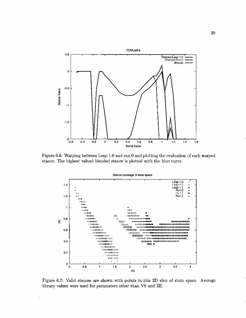
6.6 Warping between Leap 1.0 and Run 0 .. . . . . . . . . 39

6.7 State space slice through VS and ZE with only warping 39

6.8 State space slice through VS and ZE with blending . . . 40

6.9 Few stances, many blends technique used varying VS. The height of the

surface points is the stance's value. . . . . . . . . . . . . . . . . . . . . . .. 41

vii

6.10 Few stances, many blends technique used varying VE. The height of the

surface points is the stance's value. . . . . . . . . . . . . . . . . . . . . . .. 41

6.11 Few stances, many blends technique used varying ZE. The height of the

surface points is the stance's value. . . . . . . . . . . . . . . . . . . . . . .. 42

6.12 Many stances, few blends technique used varying ZS. The height of the sur­

face points is the stance's value. . . . . . . . . . . . . . . . . . . . . . . . .. 42

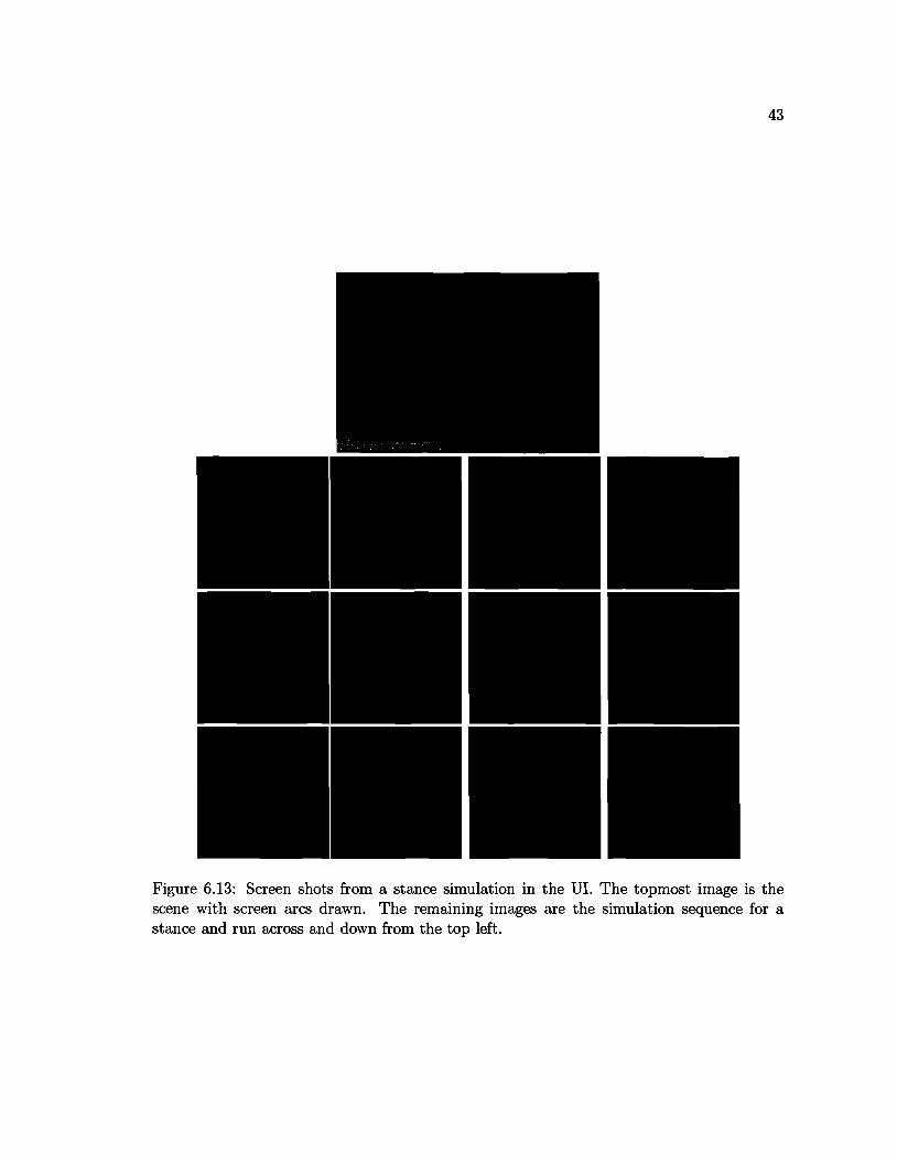
6.13 Screen shots from a stance simulation in the UI. The topmost image is the

scene with screen arcs drawn. The remaining images are the simulation

sequence for a stance and run across and down from the top left. . . . . .. 43

7.1 Unimplemented support polygon blending. . . . . . . . . . . . . . . . . .. 45

7.2 State space coverage idea. 2D slice of state space with coverage areas deter­

mined, also in 2D. 46

7.3 Adjustable velocity vectors in the UI 47

viii

Chapter 1

Introduction

Computer animators are often artists who painstakingly move articulated figures into key

poses for motion sequences. This process of key-framing can be extremely time-consuming,

while a similar motion could probably be created much more simply by using motion cap­

ture. Motion capture forces the motion to adhere to the laws of physics, because an actor

generates the motion data by actual performance.

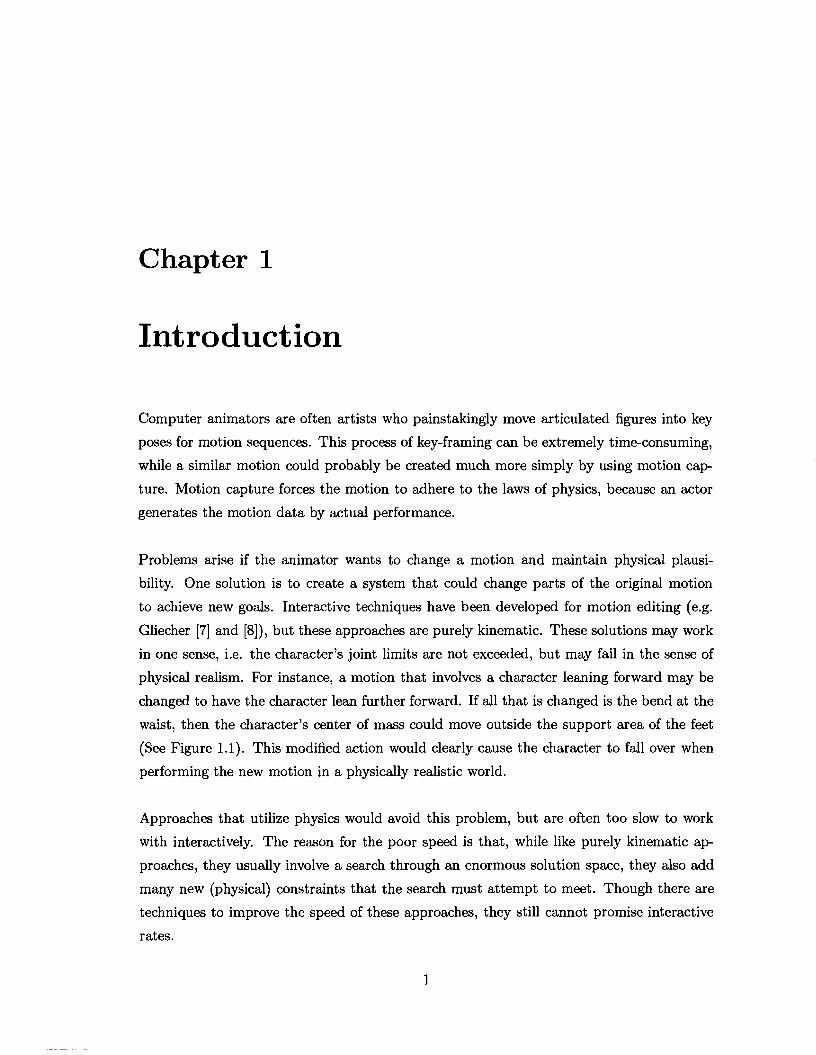
Problems arise if the animator wants to change a motion and maintain physical plausi­

bility. One solution is to create a system that could change parts of the original motion

to achieve new goals. Interactive techniques have been developed for motion editing (e.g.

Gliecher [7] and [8]), but these approaches are purely kinematic. These solutions may work

in one sense, i.e, the character's joint limits are not exceeded, but may fail in the sense of

physical realism. For instance, a motion that involves a character leaning forward may be

changed to have the character lean further forward. If all that is changed is the bend at the

waist, then the character's center of mass could move outside the support area of the feet

(See Figure 1.1). This modified action would clearly cause the character to fall over when

performing the new motion in a physically realistic world.

Approaches that utilize physics would avoid this problem, but are often too slow to work

with interactively. The reason for the poor speed is that, while like purely kinematic ap­

proaches, they usually involve a search through an enormous solution space, they also add

many new (physical) constraints that the search must attempt to meet. Though there are

techniques to improve the speed of these approaches, they still cannot promise interactive

rates.

1

2

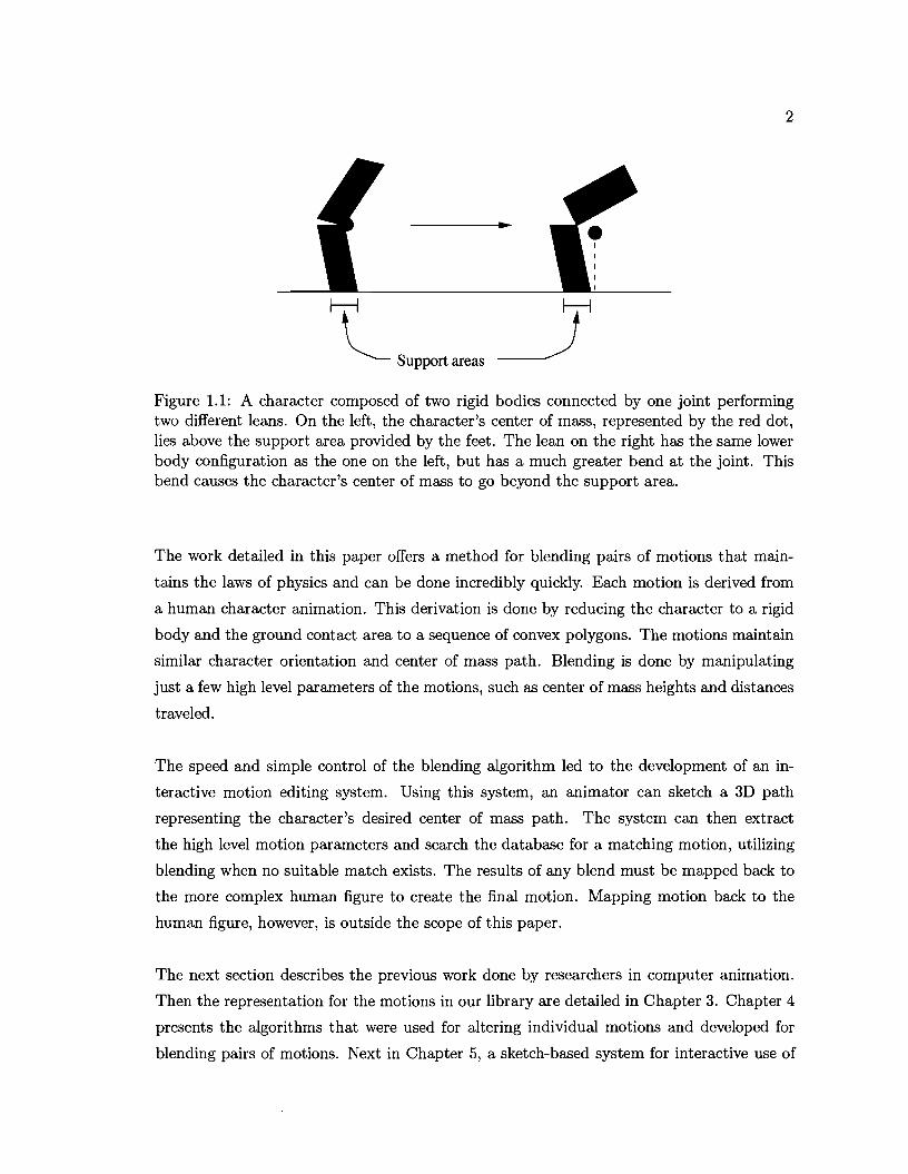
I ~ Supportareas ~ I Figure 1.1: A character composed of two rigid bodies connected by one joint performing two different leans. On the left, the character's center of mass, represented by the red dot, lies above the support area provided by the feet. The lean on the right has the same lower body configuration as the one on the left, but has a much greater bend at the joint. This bend causes the character's center of mass to go beyond the support area.

The work detailed in this paper offers a method for blending pairs of motions that main­

tains the laws of physics and can be done incredibly quickly. Each motion is derived from

a human character animation. This derivation is done by reducing the character to a rigid

body and the ground contact area to a sequence of convex polygons. The motions maintain

similar character orientation and center of mass path. Blending is done by manipulating

just a few high level parameters of the motions, such as center of mass heights and distances

traveled.

The speed and simple control of the blending algorithm led to the development of an in­

teractive motion editing system. Using this system, an animator can sketch a 3D path

representing the character's desired center of mass path. The system can then extract

the high level motion parameters and search the database for a matching motion, utilizing

blending when no suitable match exists. The results of any blend must be mapped back to

the more complex human figure to create the final motion. Mapping motion back to the

human figure, however, is outside the scope of this paper.

The next section describes the previous work done by researchers in computer animation.

Then the representation for the motions in our library are detailed in Chapter 3. Chapter 4

presents the algorithms that were used for altering individual motions and developed for

blending pairs of motions. Next in Chapter 5, a sketch-based system for interactive use of

3

the blending and warping algorithms is presented. Results from blending and the interactive

system are presented in Chapter 6, and finally, there is a discussion of the issues that were

encountered as well as points for future development located in Chapter 7.

Chapter 2

Previous Work

Work in computer animation, specifically animation of human characters, can be viewed,

most generally in two categories: motion creation and motion editing.

2.1 Motion Creation

There have been four main approaches to creating motion: key-framing, motion capture,

physical simulation, and constrained optimization.

The first approach is called key-framing and involves the specification of poses for "key"

frames by a skilled animator. The joint parameters specified in the key-frames are then

interpolated to find the poses for all frames between. An animator can edit poses kine­

matically, by directly altering parameters, or inverse kinematically(IK), by repositioning

end-effectors. Zhao and Badler [26] did work on IK for highly articulated figures. Using IK

makes for a much more intuitive interface for animators. With IK, a solver computes the

necessary angles between connected bodies to maintain the end-effectors' positions, as the

user defined. This technique does not ensure physical realism, and is most effective when

that is not desired. The next three methods of motion creation do, or can be made to,

preserve the laws of physics.

Another approach, which has become more popular as the cost and difficulty have de­

creased, is motion capture. An actor is typically wired with sensors, before performing the

desired motion. The joint parameters are computed for each frame using the sensor data.

Ascension Technology Corp. [1] and InterSense, Inc. [12] are two of the many companies

that manufacture motion capture equipment.

4

5

A third approach is to create a control system to generate a particular motion in physical

simulation. The control system examines the current state of the character and decides the

appropriate force(s) and joint torques to apply. Raibert and Hodgins [18] produced control

systems to create legged locomotion for a monoped, biped, and quadraped. Hodgins, et

al. [11] created control systems for running, cycling, and vaulting motions for human-like

characters. A great feature of this approach is that it is physically realistic. It also achieves

the goal of appearing natural, because the control system is developed by analyzing an

actual human's motion.

There are a number of disadvantages to using control systems for animation. It is often

extremely time-consuming to run the simulations. It is also difficult to create a control

system. The creator must have a fairly detailed knowledge of the human motion, and often

must painstakingly tweak parameters to get a working controller.

The last approach is to formulate the motion creation as a constrained optimization prob­

lem. This was done most notably by Witkin and Kass [23], who coined the term spacetime

constraints. An animator specifies goals of the motion, such as height or length of a jump

and contact points. These goals are then treated as constraints, and therefore must be satis­

fied by the spacetime solver. The animator also creates an objective function, i.e. minimize

total joint motion. The solver then attempts to minimize or maximize the objective func­

tion while satisfying the constraints. A great advantage of this technique is that it solves

for the entire motion simultaneously, rather than one frame at a time, as with a standard

IK solution.

On the other hand, the key problem with this approach is the amount of time required

for the solver to converge on a solution. For this reason, it has not been useful for long

animation sequences or human animation without a good deal of character simplifications.

There has been a considerable effort in speeding it up, though. Cohen [5] introduced a

technique to use spacetime constraints over a longer animation sequence than previously

possible, by breaking the sequence up into spacetime windows. He also discusses an inter­

active system that allows the user to specify constraints and optimization functions and to

guide the optimization process. Two years later, Liu, Gortler, and Cohen [15] developed a

method to speed the convergence of a spacetime solver by reducing the number of discrete

variables involved. They used a hierarchical, wavelet basis, representation of joint angle

6

curves to accomplish this.

2.2 Motion Editing

Most recent research in human character animation has focused on motion editing. The

ability to edit motion efficiently and effectively is essential to animators.

Recorded motions are typically only useful for one particular character. In order to reuse

motion for a new character, some adaptation must be performed. Hodgins and Pollard [10]

presented a method for adapting a control system developed for one character to another.

The control parameters are scaled based on geometry, mass, and moment of inertia of the

two characters, and a simulated annealing search tunes the system to the new character.

Gleicher [8] followed with a spacetime solver that treats the user-defined important aspects

of the motion as constraints while minimizing the introduction of additional artifacts.

Because, for every motion, each joint parameter curve is essentially a signal, some editing

approaches have utilized signal processing algorithms. Bruderlin and Williams [3] applied

some of these signal processing techniques to motion editing. Specifically, the authors intro­

duced multiresolution filtering of joint parameter curves, multi-target motion interpolation

with time-warping for blending motions, and motion displacement maps.

One extremely popular approach to motion editing is the use of spacetime constraints to

satisfy animator-specified changes to and minimize difference from the original motion.

Spacetime constraints and motion displacement maps are combined by Gleicher [7] and

Lee and Shin [14] for different approaches to motion editing. Rose, et al [20] used space­

time constraints to create transitions between existing motions. Popovic and Witkin [17]

simplified the character from the original animation and added dynamics to the spacetime

formulation. The spacetime solution is then fitted back to the original character.

A variety of other techniques, presented in [21] [24] and [13], have been employed to edit

motion. Unuma, et al [21] used the Fourier expansions of the joint parameter curve samples

to define a functional character model. Then using Fourier series expansions, the authors

could generate interpolation, extrapolation, and transition between motions, plus control

the "mood" of motions. The same year, Witkin and Popovic [24] described a motion warping

7

technique that deformed joint parameter curves smoothly, while preserving the subtleties

of the original curves. An animator could edit keyframes to drive the warping process.

Lamouret and van de Panne [13] allowed an animator to layout a desired motion, while

their system searched a motion database for the closest matches. The matches were then

adapted, minimizing the displacement of the initial and final positions, given the terrain

and unadapted, original motion from the databse.

In [22], van de Panne generated animation for bipedal creatures given footprints and timing

information. An optimization function was used to maximize physical realism and "com­

fort" in determining the character's center of mass motion path. Rose, et al [19] performed

interpolation of existing motions over multiple dimensions(physical & emotional characteris­

tics) using radial basis functions. Gleicher and Litwinowicz [9] combined a constraint-based

method with motion-signal processing methods to adapt motion to new characters and sit­

uations. Most recently, Pollard and Behmaram-Mosavat [16] extracted the task model from

a motion for editing. The process that they used adheres to constraints, i.e, contact point

position and friction limits, while maintaining physical realism.

This paper focuses on motion editing rather than creation, so the goal is to maximize

the usefulness of a small database of existing motions for animation. Similar to the other

motion editing approaches, the goal is to alter motions from the database to suitably fit

new situations. Our approach to the problem involves a library of physics-based motions

and warping and blending operations that can adapt each motion to different situations

without the extensive search required by spacetime constraints approaches. These motions

are represented as "stances", and are detailed in the next section. Warping a stance means

that it is altered to display some new physical characteristics, without losing its stylistic

sublteties. Blending two stances generates a new stance with physical properties and stylistic

qualities that are a mix of the original stances. The warping and blending processes are

described in detail in Sections 4.1 and 4.2 respectively.

• •

launch ze

Chapter 3

Introduction to Stances

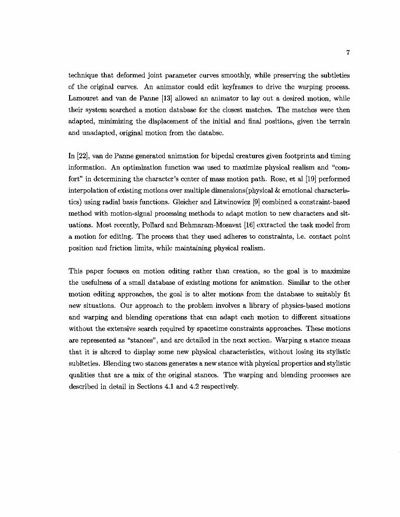
vertical

a. b.

landing

/ contact J L x ~II"

heading

Figure 3.1: Stance example - a) The center of motion path for a stance, where the green dots are the flight apexes and the ground phase occurs between landing and launch. b) There are six parameters that define each stance. Five of them are shown here, while the end velocity in the perpendicular direction, vp, is normal to the paper and not shown.

While motion editing encompasses many general problems, this work was focused on motion

that can be represented as a sequence of stances. Each stance is defined as being between

the apexes of two consecutive flight phases and containing one ground phase (Figure 3.1a).

Running and jumping are both good examples of motion that can be approximated in this

way. The "Stances as Units of Motion" ideas and libraries were created by Nancy Pol­

lard [16].

8

9

3.1 Parameters

Every stance is defined by six parameters, which are described in Table 3.1 and exemplified

in Figure 3.1b. Each of the stances has its own coordinate frame and local timing infor­

mation. The coordinate frame is composed of the heading, vertical, and the perpendicular

directions. The heading direction is the horizontal component of the character's velocity

vector at the start of the stance.

As I described above, each stance runs between one flight apex and the next flight apex. It

begins at the first apex, at time 0, and continues in the flight phase until contact is made

with the ground. Contact is maintained until launch, which moves it back into flight.

Table 3.1: Stance parameter descriptions. ZS Position in the vertical direction at the first

apex (start of the stance) ZE Position in the vertical direction at the second

apex (end of the stance) VS Velocity in the heading direction at the first

apex (start of the stance) VE Velocity in the heading direction at the second

apex (end of the stance) VP Velocity in the perpendicular direction at the

second apex (end of the stance) X Distance in the heading direction from the

first apex to the second

3.2 Forces and Torques

External force, [, and torque, T, are applied to the character at each simulation timestep

during ground contact. Each of our stances began as either motion capture data or a

keyframed animation. In either case, a center of mass (COM) for the character could be

determined for each frame; and hence, the COM path could be determined over the entire

motion. By numerically differentiating this twice, we get acceleration and can extract a

first guess at the forces necessary to produce the given COM path at discrete timesteps.

This acceleration is rotated into the character's coordinate system (vertical, heading, and

perpendicular) and multiplied by the character's mass, giving us the total force applied.

10

This force is sampled at N discrete timesteps using the following equation:

FTU) = mi (to + j~t), j = 0, ... , N - 1

where the stance starts at time to and lasts for time /.),.t. This initial guess at contact forces

is then refined using a search technique that ensures that the body's position and orien­

tation match the reference motion as well as possible. This search technique also extracts

applied ground torque.

Next, a Discrete Fourier Transform (DFT) is used to approximate the forces. The dominant

terms of the DFT are kept and used in simulation of the character for each stance. The

applied force is then given by the equation:

(3.1)

y(t)

P• s

Q4

•Po •

P2 .. x(t)

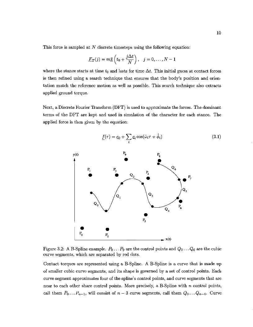
Figure 3.2: A B-Spline example. Po ... Pg are the control points and Qo ... Q6 are the cubic curve segments, which are separated by red dots.

Contact torques are represented using a B-Spline. A B-Spline is a curve that is made up

of smaller cubic curve segments, and its shape is governed by a set of control points. Each

curve segment approximates four of the spline's control points, and curve segments that are

near to each other share control points. More precisely, a B-Spline with n control points,

call them Po ... Pn-l, will consist of n - 3 curve segments, call them Qo ... Qn-4. Curve

11

segment Qi is then defined by control points Pi, Pi+1, ~+2, Pi+3. This formulation implies

that segment Qi+l will share 3 of the control points defining Qi, namely Pi+1, Pi+2, and

Pi+3. In Figure 3.2, there is an example of a B-Spline with its control points and curve

segments labeled. The curve segments are separated by red dots, and the numbering scheme

for them and the control points is as described above.

A critical feature of a B-Spline is that it has C 2 continuity, meaning that the first and

second derivatives are defined over the entire curve. This is true because curve segments

share control points.

Note that blending stances will require both algorithms for blending the DFT representa­

tions of forces and for blending the B-Spline representations of contact torques.

Chapter 4

Motion Blending Algorithms

A library of unaltered stances, no matter how large, could not be complete. As stated in

Chapter 3, each stance is defined by a set of six parameters, and is essentially represented

by a point in the state space. So the state space could not be covered by any finite number

of stances. This has driven us to find methods for altering stances to fill in gaps in the

state space when necessary. The next section starts with a warping technique, which can

alter a given stance to place it anywhere in the state space, developed by Nancy Pollard [16].

4.1 Warping a Stance

Altering a stance involves scaling the applied forces by a diagonal matrix. The scale matrix

{3 is applied as such,

(4.1)

Each force L in the equation is a vector with a vertical, heading, and perpendicular compo­

nent, while !i has only vertical, heading, and perpendicular diagonal entries. Subtleties of

the original motion should remain unchanged because we are only scaling the forces.

In order to create the new, scaled stance, the three scale factors must be determined, and

landing and launch times must be adjusted. Given a set of six desired stance parameters,

we have a fully determined set of equations to solve for the scales and timing information.

Start by letting the stance begin at time 0, and defining variables tTD = landing time, tLO

= liftoff time, and tE = end time at the end of the stance. The ground time, call it At, for

12

13

a stance is not changed by warping. So the same adjustment is made to tLO and tTD, and

we have:

(4.2)

Equation (3.1) from Chapter 3 can be rewritten to yield:

where actual time, t, is used instead of normalized time, r. We find the change in velocity

by integrating this equation from time tTD to tLO and dividing through by the mass. This

is given by: . . f3ffJD.t ;?2(tLO) - ;?2(tTD) = --- + gD.t

m -

Then, the ballistic segments of the stance are added, yielding:

f3ffJD.t 42(tE) - 42(0) = --- + gtE

m -

So, now we can find equations for the stance parameters. They are:

f3hCO,hD.tve ­ VB = (4.3)

m

vp f3pco,pD.t

m (4.4)

gtE = f3vco,vD.t m

(4.5)

where the subscripts h, V, and p stand for the heading, vertical, and perpendicular directions

respectively. The gravity vector

with the final position represents the vertical direction.

Integrating the velocities between two apexes gives us the change in position from the first

to the second apex. The equation we get is:

14

Again, we need to put this in terms of stances parameters to solve for the unknowns. Now

we have:

(4.6)

(4.7)

Equations (4.2), (4.3), (4.4), (4.5), (4.6), and (4.7) are then solved for tTD, tLO, te, {3h, {3v,

and (3p, giving us the new scale factors and timing information.

While altering stances does help to fill in the space of stances, it often cannot fill enough.

That's where blending comes in. It is extremely useful for filling gaps between stances in

the state space. The blending algorithm is described in the next section.

Stances can be warped to any parameters in the state space; however, many physically

implausible stances could be generated by the outlined process. Physical realism is not a

constraint in the scale factor problem, so it is easily violated. A method for evaluating a

stance's physical realism was developed and is detailed in Section 4.3.

4.2 Blending Stances

The blending algorithm takes two stances and a blend value, which is denoted by k through­

out this section, and outputs a blended stance. In general k is used for interpolation, i.e,

o~ k ~ 1, but it could be used for extrapolation, when k < 0 or k > 1. The blend value,

k, refers to the amount of the first stance that is blended with 1 - k of the second stance.

Equation (4.8) uses the blend value and is applied to all stance characteristics, except the

first three, listed in Table 4.1 Because the ground time is just a constant, equation (4.8)

can be directly applied to the value, but in the case of vector types, the equation must be

applied to each scalar component of the vector.

Gn ew = (k· GA) + ((1 - k) . GB) (4.8)

Here, G* is the characteristic being blended and the subscript refers to the stance.

The next two sections discuss the two larger pieces of the stance blending algorithm. The

first is a method for blending ground torque (B-Splines), and the second describes the blend­

ing of applied force (DFTs). Support polygon's were not blended, but were selected from

15

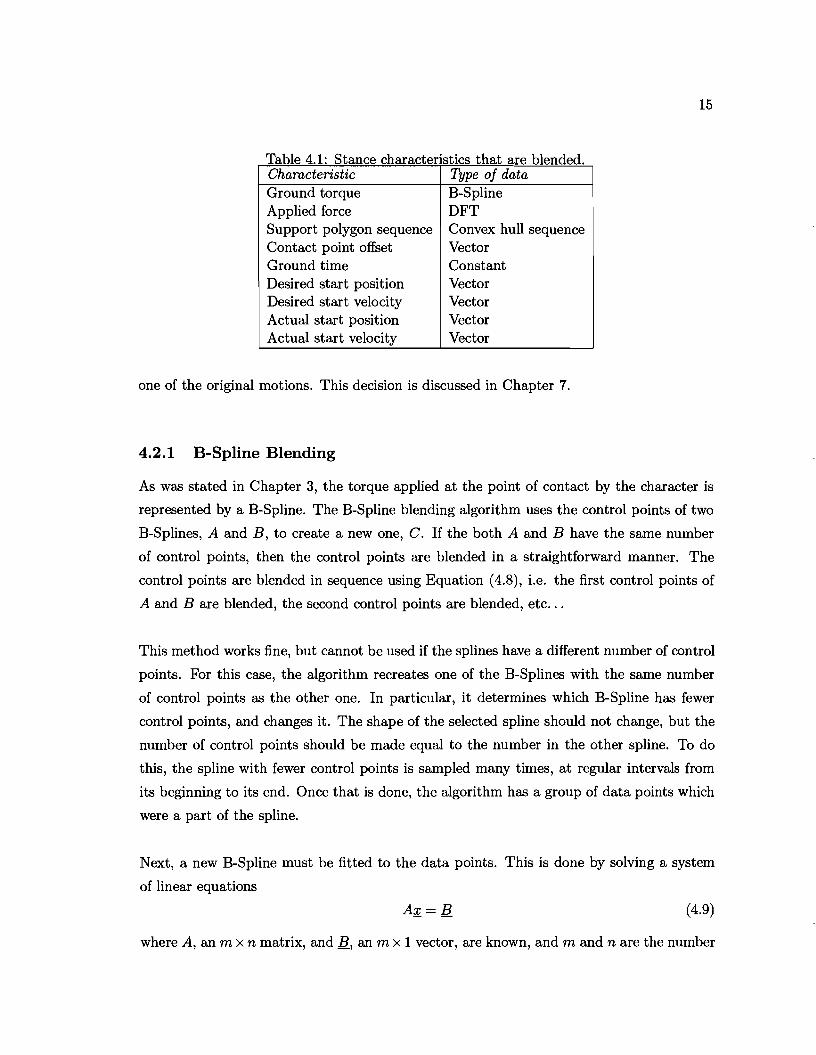
Table 4 I: Stance characteristics that are blended .. Characteristic Ground torque Applied force Support polygon sequence Contact point offset Ground time Desired start position Desired start velocity Actual start position Actual start velocity

Type of data B-Spline DFT Convex hull sequence Vector Constant Vector Vector Vector Vector

one of the original motions. This decision is discussed in Chapter 7.

4.2.1 B-Spline Blending

As was stated in Chapter 3, the torque applied at the point of contact by the character is

represented by a B-Spline. The B-Spline blending algorithm uses the control points of two

B-Splines, A and B, to create a new one, C. If the both A and B have the same number

of control points, then the control points are blended in a straightforward manner. The

control points are blended in sequence using Equation (4.8), i.e. the first control points of

A and B are blended, the second control points are blended, etc...

This method works fine, but cannot be used if the splines have a different number of control

points. For this case, the algorithm recreates one of the B-Splines with the same number

of control points as the other one. In particular, it determines which B-Spline has fewer

control points, and changes it. The shape of the selected spline should not change, but the

number of control points should be made equal to the number in the other spline. To do

this, the spline with fewer control points is sampled many times, at regular intervals from

its beginning to its end. Once that is done, the algorithm has a group of data points which

were a part of the spline.

Next, a new B-Spline must be fitted to the data points. This is done by solving a system

of linear equations

A;r= B (4.9)

where A, an m x n matrix, and B, an m x 1 vector, are known, and m and n are the number

16

of sample points and the desired number of control points respectively.

In our case, the vector B is filled with the m sampled data points, and the matrix A is

derived from the B-Spline equations. A has the following form:

a b c d 0 A= (4.10)

[ o . ~ ] and the letters in Equation (4.10) stand for

a 1 (3 2"6 -t + 3t )- 3t + 1

b ~ (3t3 - 6t2 + 4)

c ~ (-3t3 + 3t2 + 3t + 1)

d ~ (t3 )

We solve for ;£, which will contain the n control points for the new spline. Now we have two

splines with the same number of control points, and the first B-Spline blending algorithm

can be applied.

4.2.2 DFT (Force) Blending

Ground torque applied is one aspect of a stance, but perhaps a more important one is the

force applied. The forces applied at the single contact point are described by the dominant

terms of the DFT used to interpolate the original discrete forces. This is described in detail

in Chapter 3. So, the next step in blending stances involves blending DFTs.

The key to blending DFTs is to blend terms that have the same frequencies with each

other. The single DFT terms that I am refering to are contained in the summation in

Equation (3.1). So the i th term in stance A's DFT looks like

where the w represents the frequency of each DFT term and the superscript, (A), denotes

the stance. Note: Similar notation is used throughout this section.

Each pair of same frequency terms of the DFT (one from each stance) can be blended

together to create a DFT term for the blended stance's applied force. The blend can be

17

performed by applying equation (4.8) to each coefficient, Ci of the DFT term. If there

is a particular DFT frequency that only one of the two stances contains, then the term

containing that frequency is blended with a zero term. For example, if for some i, w;A) = 4

(stance A has a frequency of 4) and stance B has no term with a frequency of 4, then the

blended term is just

DFT~C) = k . c~A) cos (jA)r + A.~A))--3 -t t 'f't

where k is the blend value.

4.3 Stance Evaluation

The goal of blending stances is to fill in gaps in the state space, so that the motion library

is more complete. As I stated before, any stance can be warped, and any warped stances

can be blended. The results from blends of randomly warped stances will vary in physi­

cal plausibility. That, combined with the fact that physically implausible stances are not

valid in the stance library, shows that it is important to be able to evaluate blended stances.

The evaluation method only examines a few physical characteristics of the stance, ignoring

any stylistic characteristics. For example an artistically pleasing stance may involve the

leg that is in contact with the ground reaching full extension on lift off. Another issue in

the evaluation is that there is limited available, physical information about the character

in each stance. Because the human character is treated as a single rigid body, we can only

examine the center of mass position, the contact point, and the forces and torques applied

at that point. For instance, limits on joint angles and torques cannot be enforced in the

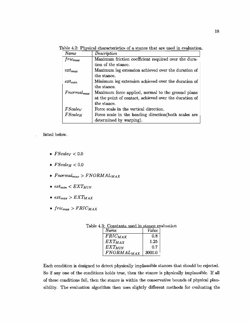
evaluation. The physical characteristics that are used are listed in Table 4.2.

The primary goal of this evaluation algorithm is to reject physically implausible stances. It

may often be necessary to rate stances, rather than just accept or reject them.

To determine physical plausibility and evaluate a stance, the algorithm initially assumes

that all stances are unrealistic. This means that a stance's value, call it val, is initialized

to be 0.0.

The algorithm then proceeds by checking the stance's characteristics as described in Ta­

ble 4.2. The values are compared to constants, displayed in Table 4.3, using the conditions

18

Table 4.2: Physical characteristics of a stance that are used in evaluation. Name Description fricmax Maximum friction coefficient required over the dura­

tion of the stance. Maximum leg extension achieved over the duration of the stance.

extmax

Minimum leg extension achieved over the duration of the stance.

extmin

Fnarmalmax Maximum force applied, normal to the ground plane at the point of contact, achieved over the duration of the stance. Force scale in the vertical direction. FScalev Force scale in the heading direction(both scales are determined by warping).

FScaleH

listed below.

• FScalev < 0.0

• FScaleH < 0.0

• Fnarmalmax > F NORMALMAX

• extmin < EXTMIN

• extmax > EXTMAX

• fricmax > FRICMAX

Table 4.3' Constants used in stance evaluation Name Value FRICMAx 0.8 EXTMAX 1.25 EXTMIN 0.7 FNORMALMAx 3000.0

Each condition is designed to detect physically implausible stances that should be rejected.

So if anyone of the conditions holds true, then the stance is physically implausible. If all

of these conditions fail, then the stance is within the conservative bounds of physical plau­

sibility. The evaluation algorithm then uses slightly different methods for evaluating the

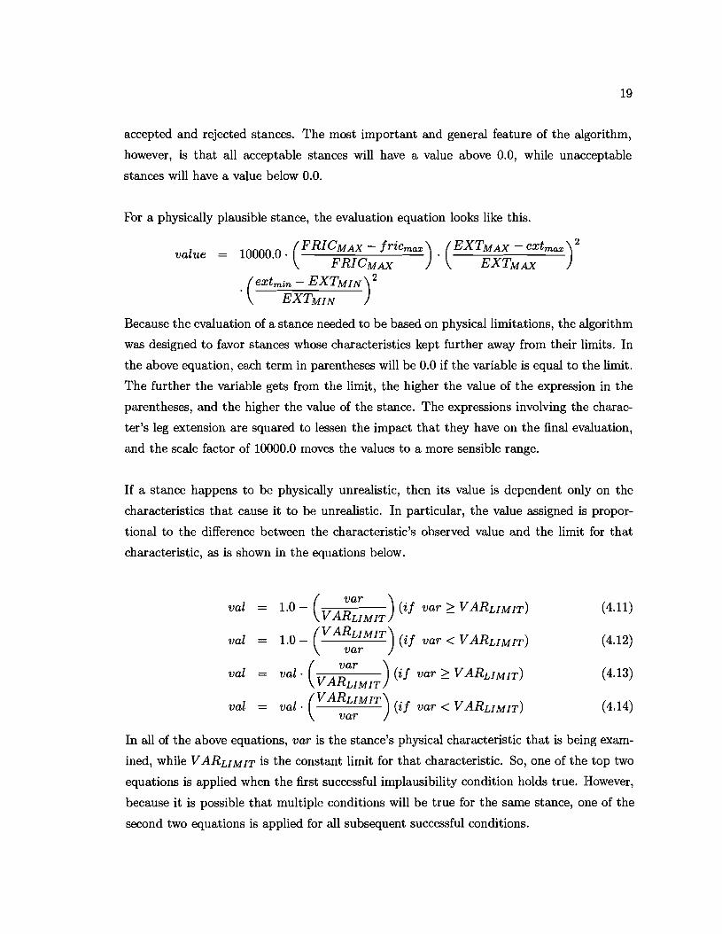
19

accepted and rejected stances. The most important and general feature of the algorithm,

however, is that all acceptable stances will have a value above 0.0, while unacceptable

stances will have a value below 0.0.

For a physically plausible stance, the evaluation equation looks like this.

value = 10000.0. (FRICMAX ­ friCmax) FRICMAX

. (EXTMAX ­ extmax) 2

EXTMAX

. (extmin - EXTMIN)2 EXTMIN

Because the evaluation of a stance needed to be based on physical limitations, the algorithm

was designed to favor stances whose characteristics kept further away from their limits. In

the above equation, each term in parentheses will be 0.0 if the variable is equal to the limit.

The further the variable gets from the limit, the higher the value of the expression in the

parentheses, and the higher the value of the stance. The expressions involving the charac­

ter's leg extension are squared to lessen the impact that they have on the final evaluation,

and the scale factor of 10000.0 moves the values to a more sensible range.

If a stance happens to be physically unrealistic, then its value is dependent only on the

characteristics that cause it to be unrealistic. In particular, the value assigned is propor­

tional to the difference between the characteristic's observed value and the limit for that

characteristic, as is shown in the equations below.

( var )val = 1.0 - V ARLIMIT (if var 2: V ARLIMIT) (4.11)

(VARLIMIT) .val = 1.0 - (1,f var < V ARLIMIT) (4.12)var

( var )val = val- V ARLIMIT (if var 2: V ARLIMIT) (4.13)

(VARLIMIT)val = val· (if var < V ARLIMIT) (4.14) var

In all of the above equations, var is the stance's physical characteristic that is being exam­

ined, while V ARLIM IT is the constant limit for that characteristic. So, one of the top two

equations is applied when the first successful implausibility condition holds true. However,

because it is possible that multiple conditions will be true for the same stance, one of the

second two equations is applied for all subsequent successful conditions.

20

For example, say that the evaluation process has just begun for a new stance. val is

initialized to 0.0, and the stance's physical characteristics are determined. If the stance

first fails the friction coefficient test, then that means,

fricmax > FRICMAx

and so, Equation (4.11) is applied with friCmax and FRIeL/MIT replacing var and V ARL/MIT

respectively. If, the next condition, say the minimum leg extension one, is also successful,

then

extmin < EXTMIN

and Equation (4.14) is applied.

Chapter 5

Interactive Motion Editing

Algorithms

Blending motions and evaluation of the new motions are both useful tools for motion editing

and they can be done very quickly. Also, the warping and blending algorithms use very in­

tuitive characteristics (positions, velocities, and distance). These qualities somewhat imply

that the techniques could be used interactively. So a system to use blending and warping

interactively was developed.

The user interface design for this system is discussed in Sections 5.1 and 5.2. Section 5.3

discusses the use of automated blending to find stances that best fit what the user desires.

5.1 User Interface

The UI was designed to be as intuitive and as simple as possible. The most logical input

was a 3D flight path for the character to follow. So, the user is only required to use the

mouse, usually drawing strokes on the screen. This appeared to be the easiest way for the

user to convey his or her desired motion for the character.

Figures 5.1 and 5.2 show example input of a flight stroke and shadow stroke in the imple­

mented system, while figure 5.3 shows the parabolas created as a result of the two curves.

To start, a user draws a motion path for the character. This is the desired path for the

21

22

Figure 5.1: UI step 1 - Draw the desired COM path, shown in red, as drawn by a user.

character's center of mass(COM) for a motion sequence. After the motion path curve is

drawn, the user draws a shadow stroke. This is treated as the shadow of the motion path

as it would appear on the ground. At any time during this process of drawing paths and

shadows, the user is able to delete the prior stroke by scribbling on it. More about useful

editing techniques is deferred to Chapter 7.

Once a motion path and its shadow are drawn, the path is projected into 3D, and a parabola

is fit to each flight phase. An explanation of this process appears in Section 5.2. Note that

every motion path is required to have a corresponding shadow, and the user isn't permitted

to proceed if just one of these two stroke types is drawn.

Whenever the projection process is done, the system checks the number of flight phases that

were detected in the motion path. If there are at least two, the user can declare him/herself

done with path editing with a click of the mouse. The reason for the requirement is that

at least two flight phases/apexes are necessary to define a stance object(refer to Chapter 3)

and hence, a set of state space parameters. So, after the single mouse click, the system

extracts the state space parameters from the curve segments. This is also described in more

detail at the end of Section 5.2

23

Figure 5.2: VI step 2 - Draw a shadow for the COM path, shown in blue, also as drawn by a user.

Once the parameters are extracted, the system must find stances to fit them. There are a

number of different methods to do this. They are described in Section 5.3.

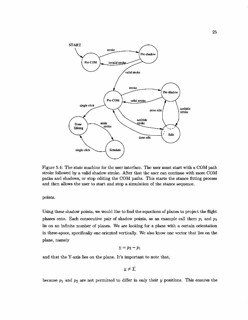
The user interface for the motion editing system acts as a finite state machine, which can

be seen in Figure 5.4, behind the scenes. This picture offers more specific details than I

have described here.

5.2 3D Curve Sketching

The main issue in the user interface design was to allow the user to sketch the desired flight

path for the rigid body in 3D, using only a 2D input device(mouse). The inspiration for

this algorithm was the 3D curve sketching system developed by J. Cohen and described in

[4]. Given a motion path sketched in screen coordinates, and a shadow for that path also

sketched in screen coordinates, this algorithm must construct a 3D representation of the

flight phases for the rigid body. Physics tells us that the motion path of the character in

flight will be planar and follow a parabola. The fact that the flight is planar is key to the

algorithm, while the parabolic shape of the flight is used to redraw the 3D curve and better

24

Figure 5.3: VI Result - 3D, parabolic curve segments are output to the screen, again shown in red.

approximate the flight apex. I will talk more about this later in this section.

The first step of the algorithm is to find the plane equations for the 2D to 3D projection.

To do this the algorithm first searches the motion path for local minima, as shown in Fig­

ure 5.5a. The purpose of this is to find approximate ground contacts, each of which will

typically appear near the local minimum between two flight phases. Each set of points

between consecutive local minima form a separate curve segment and will be treated sepa­

rately in later processes.

Using each of the minima of the motion path, the algorithm searches the shadow path

for the point nearest in the horizontal direction (Figure 5.5b). The resultant points of the

shadow path are then treated as approximate contacts on either side of a flight phase. Every

shadow point that is selected is projected into the scene and tested for intersection with

the objects (treated as ground for the character) within that scene. If all selected points

can be projected onto some geometry in the scene, then the process proceeds; otherwise,

the user is asked to redraw the shadow curve. So now each local minimum from the motion

path directly corresponds to a point on the 2D shadow line, and we can treat the separate

curve segments from the motion path as lying between two particular, consecutive shadow

25

scribble stroke

Figure 5.4: The state machine for the user interface. The user must start with a COM path stroke followed by a valid shadow stroke. After that the user can continue with more COM paths and shadows, or stop editing the COM paths. This starts the stance fitting process and then allows the user to start and stop a simulation of the stance sequence.

points.

Using these shadow points, we would like to find the equations of planes to project the flight

phases onto. Each consecutive pair of shadow points, as an example call them PI and P2

lie on an infinite number of planes. We are looking for a plane with a certain orientation

in three-space, specifically one oriented vertically. We also know one vector that lies on the

plane, namely

3!. = P2 - PI

and that the Y-axis lies on the plane. It's important to note that,

because PI and P2 are not permitted to differ in only their y positions. This ensures the

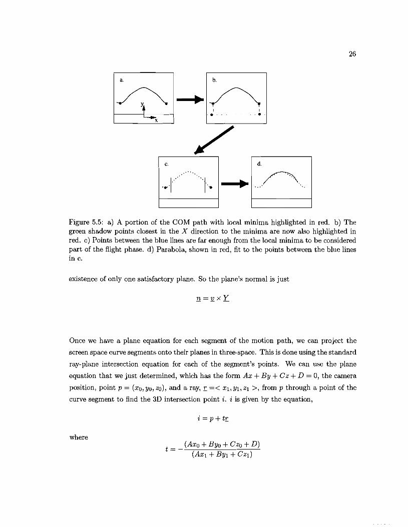
26

a. b.

I I.. . . . . ..

c. . ...

d.

r>.

Figure 5.5: a) A portion of the COM path with local minima highlighted in red. b) The green shadow points closest in the X direction to the minima are now also highlighted in red. c) Points between the blue lines are far enough from the local minima to be considered part of the flight phase. d) Parabola, shown in red, fit to the points between the blue lines mc.

existence of only one satisfactory plane. So the plane's normal is just

Once we have a plane equation for each segment of the motion path, we can project the

screen space curve segments onto their planes in three-space. This is done using the standard

ray-plane intersection equation for each of the segment's points. We can use the plane

equation that we just determined, which has the form Ax + By + Cz + D = 0, the camera

position, point p = (xo, Yo, zo), and a ray, r. =< Xl, YI,zl >, from p through a point of the

curve segment to find the 3D intersection point i. i is given by the equation,

i = p + tt:

where t = _..:....(A----,x----,o_+_B----=-::Yo::-+_C_z=o_+-,--D--:....)

(AXI + BYI + CzI)

27

So, once each point of all the curve segments has been projected, we have the user's sketched,

3D COM path. The next step is to fit a parabola to the flight portion of each curve segment.

First, the algorithm must determine which points of each segment are a part of the flight

phase and which are not. Deciding exactly which subset of points represents the flight

phase is impossible without a physical simulation, which cannot be done until we know

what stances the character will be using.

The flight phase points are instead approximated by comparing their distances from their

two bordering local minima and a threshhold. Each point that is at least ~ 0.32 meters

(distance squared is O.lm) away from either of the minima is considered a part of the flight

path and kept, while all others are discarded. This value was chosen because it seemed

plausible and yielded plausible results in the VI. While anyone value doesn't make sense

for all possible stances, a good average value will work in general. Figure 5.5c shows exam­

ple points of a curve segment, with the two neighboring local minima colored red, and the

distance thresholds marked by blue lines. Every point between the lines is sufficiently far

from either minimum.

Now, the algorithm must fit a parabola to the points that were kept from each flight segment.

This is done using a least squares method, which in its implementation requires 2D samples

for input. The method was designed as described in [6] pp. 768-70. Because the flight

points all lie in 3-space, but are in groups that are planar, a projection into two dimensions

is straightforward. The Y, vertical, component of the positions is retained as the Y compo­

nent in 2D. The x, horizontal, component of the points in 2D is determined by projecting

the 3D points onto the xz plane. When this projection is done, because all of the points

were on a vertical plane, they will lie on a horizontal vector. Each point's distance from

a chosen origin on this vector will be the horizontal component of the point's 2D coordinate.

Next the 2D points from each flight phase are fitted to a parabola. Fitting a parabola to

points means that the error, total distance of all points from the parabola, is minimized.

This is exactly what least squares approximation does. In our case, we choose to minimize

the error in the Y direction. So, given 2D points,

(Xl,Yl),(X2,Y2), ... (xn,Yn)

we want to find a function F(x) such that

Yi = F(Xi) + €i

28

where n-l

ET = LE; i=O

is minimized.

We are looking for F in the form of a weighted sum of basis functions. So, we want

m-l

F(x) = L Cj . h(x) j=O

and, because we are looking for a polynomial, we want the basis functions to be of the form

More specifically, we are looking for a parabola, so in our case m = 2 and we have

Now, we can set up a set of linear equations, and solve them to find our parabolic equation.

So, once again we must solve the A~ = Qequation. This time we fill a matrix A with the

values of the basis functions at our 2D data points. Then we fill Q, which has dimensions

m x 1, with our evaluations of F(x) for all data points. A, in it's general form, looks like

this fm-l(XO)

fm-l(Xl) (5.1)A=

but, our equation will look like this with matrix A filled specifically for a quadratic equation

A~=Q (5.2)

F(xo)

fO(Xl) h(Xl) !2(Xl)

fo(xo) h(xo) !2(xo)

F(Xl) (5.3)(:)~

F(xn-dfo(xn-d h(Xn-l) !2(Xn-l)

To solve equation (5.3) for ~, we must compute the pseudoinverse of the matrix, A. The

pseudoinverse of A, A+ is calculated by the equation

29

With A+ and some algebraic manipulation, we can get the equation in terms of ;f.

;f ((ATA)-l AT)Q A+Q

Having the equations for the parabola representing each flight phase is good, but we still

need 3D points on that parabola for display in the scene. The parabolic equations can each

be sampled to yield 2D points that lie in the same domain as our 2D data points prior to

fitting.

The new 2D points must then be converted into 3D to create a polyline representation in

3-space. This is done by inverting the method of projection from 3D to 2D that I described

before the least squares method. The y, or vertical, component of each point will remain

the same in 2D as it is in 3D. The x and z components of each point are calculated by

multiplying the same normalized vector from the previous projection of this point to 2D by

the it's horizontal (scalar) component. The vector lies in the xz-plane, and so this multi­

plication will yield the point's new x and z components.

Once the curve segments have been approximated by parabolas, the system can extract the

desired state space parameters(again, refer to Chapter 3). For each parabola, the system

finds its apex. Because each stance is defined as being between two apexes, if there are n

parabolas/apexes, the system will extract n -1 sets of state space parameters. The system

finds the start and end vertical positions of the stance between consecutive apexes. It also

uses the distance between apexes as the desired distance; however, the apexes cannot be used

to extract any of the necessary velocity components. Figure 5.6 provides some visualization

for this step. Extracting velocities presents a different issue, which is discussed in detail in

Chapter 7. For my system, I used average start and end velocities in the heading direction

and the end velocity in the perpendicular direction. All of the average state space parameter

values for the library are listed in Table 5.1, while the average values for just the jumping

stances are listed in Table 5.2. The second set of averages was necessary for experiments

described later.

5.3 Automated Motion Blending Algorithms

The database of stances that I used in the editing system was fairly small, in fact most

of my experiments only involved 9 different stances. While it is certainly possible that

30

~--x-----~

Figure 5.6: State space parameter extraction from parabolas

Table 5.1: Average state space parameter values for all stances Parameter Value ZS = 1.11927 m

ZE= 1.14108 m

VS = 2.65328 tti]« VE= 2.77254 tti]« VP= -0.0264183 m]s x= 1.43893 m

These values were computed based on the original state space parameters of the 6 stance library.

unchanged stances from the library would fit into the motion path, it is unlikely. Fitting

into the motion path means that a stance matches one of the state space parameter sets

exactly. It is actually much more likely that none is acceptable without alteration.

The automated blending process was created to help alleviate this problem. It performs a

simple search over the library for each state space parameter set extracted in the VI. The

process starts by warping each of the stances in the database, as described in Section 4.1,

and then evaluating the warped stances, as described in Section 4.3. If any of these stances

receives a positive evaluation(implies physical plausibility), then the one that evaluated

highest is chosen. If none are plausible, then the search continues.

Next it uses the blending algorithms from Section 4.2 to look for an appropriate stance.

The first search involves choosing only a few (m, where m 2: 2, but is small) stances from

the library and blending them together with many different fractional values. The key to

this method lies in the selection of just a few stances. Because the warped stances were just

evaluated, the algorithm chooses the m best stances for blending.

31

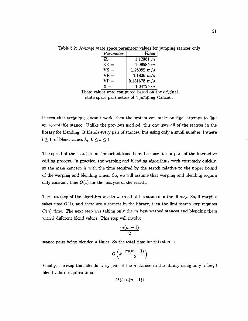
Table 5.2: Average state space parameter values for jumping stances only Parameter Value ZS = 1.12981 m ZE= 1.09585 m VS = 1.25092 m]» VE= 1.1826 m]» VP= 0.131678 m]» x= 1.04725 m

These values were computed based on the original state space parameters of 4 jumping stances .

If even that technique doesn't work, then the system can make on final attempt to find

an acceptable stance. Unlike the previous method, this one uses all of the stances in the

library for blending. It blends every pair of stances, but using only a small number, 1where

1~ 1, of blend values k, 0 ~ k ~ 1

The speed of the search is an important issue here, because it is a part of the interactive

editing process. In practice, the warping and blending algorithms work extremely quickly,

so the main concern is with the time required by the search relative to the upper bound

of the warping and blending times. So, we will assume that warping and blending require

only constant time 0(1) for the analysis of the search.

The first step of the algorithm was to warp all of the stances in the library. So, if warping

takes time 0(1), and there are n stances in the library, then the first search step requires

O(n) time. The next step was taking only the m best warped stances and blending them

with k different blend values. This step will involve

m(m -1) 2

stance pairs being blended k times. So the total time for this step is

Finally, the step that blends every pair of the n stances in the library using only a few, 1

blend values requires time

0(l·n(n-1))

32

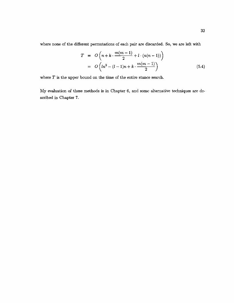
where none of the different permutations of each pair are discarded. So, we are left with

m(mT = O(n+k. 2-1)+l.(n(n-l)))

o (ln2 - (l-l)n + t«. m(m - 1)) (5.4)2

where T is the upper bound on the time of the entire stance search.

My evaluation of these methods is in Chapter 6, and some alternative techniques are de­

scribed in Chapter 7.

Chapter 6

Results

6.1 Blending

Blending was performed one of two ways, by warping and blending between two stances or

by warping to an arbitrary state space coordinate and blending. The difference between the

two methods is that the first determines intermediate stance parameters. So the warping

and blending are done along a line in the 6D state space.

Blending between stances along the 6D line was extremely important in testing the blending

algorithm, but was not used in the motion editing system. The COM path for the original

motions and blended motions could be plotted from apex to apex. It was easy to identify

the stance parameters and judge whether or not the blends looked feasible based on those.

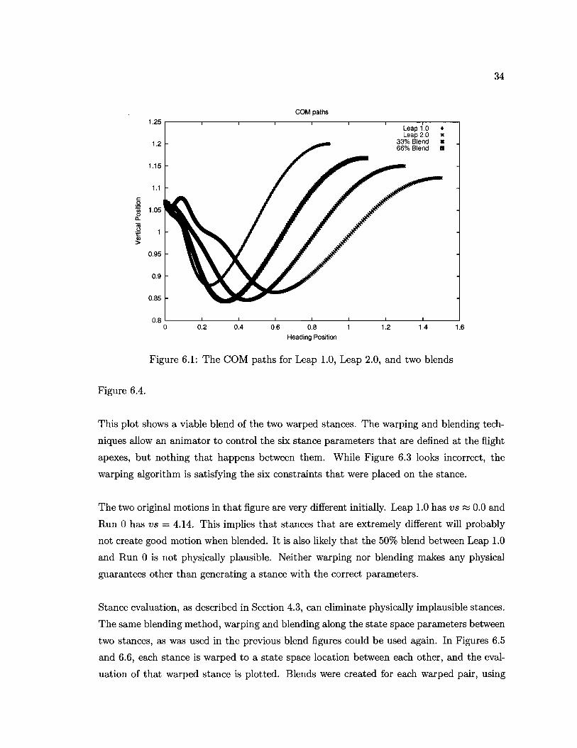
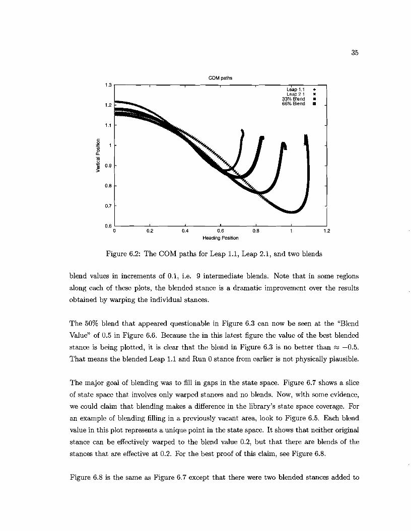
Figures 6.1, 6.2, and 6.3 all show two library motions that were were used to create inter­

mediate blends between them. The COM paths are all plotted with heading position vs.

vertical position and with the original motions drawn in red and green. A 33% blend is

33% of the motion labeled with red and 66% of the green motion.

Figures 6.1, 6.2 yield the results that one would expect from blending between two stances.

The COM paths for the blended stances lie between the the original stances, and the stance

parameters are almost exactly where they should be. Figure 6.3, on the other hand, looks

nothing like what would be expected. The stance parameters are correct for the blend, but

it appears that the stance never reaches an apex. The new stance has a landing time that is

before its first apex and a launch time that is after its next apex. For a better understanding

of what's happening, we turn to the plots of the warped stances and the blend shown in

33

34

COM paths 1.25

Leap 1.0 • Leap 2.0 x

1.2

66% Blend 33% Blend _1.2

..

1.15

1.1

c 0

'iii"" 1.05 0 a.

~ :e Ql >

0.95

0.9

0.85

0.8 0 0.2 0.4 0.6 0.8 1.4 1.6

Heading Position

Figure 6.1: The COM paths for Leap 1.0, Leap 2.0, and two blends

Figure 6.4.

This plot shows a viable blend of the two warped stances. The warping and blending tech­

niques allow an animator to control the six stance parameters that are defined at the flight

apexes, but nothing that happens between them. While Figure 6.3 looks incorrect, the

warping algorithm is satisfying the six constraints that were placed on the stance.

The two original motions in that figure are very different initially. Leap 1.0 has VB ~ 0.0 and

Run 0 has VB = 4.14. This implies that stances that are extremely different will probably

not create good motion when blended. It is also likely that the 50% blend between Leap 1.0

and Run 0 is not physically plausible. Neither warping nor blending makes any physical

guarantees other than generating a stance with the correct parameters.

Stance evaluation, as described in Section 4.3, can eliminate physically implausible stances.

The same blending method, warping and blending along the state space parameters between

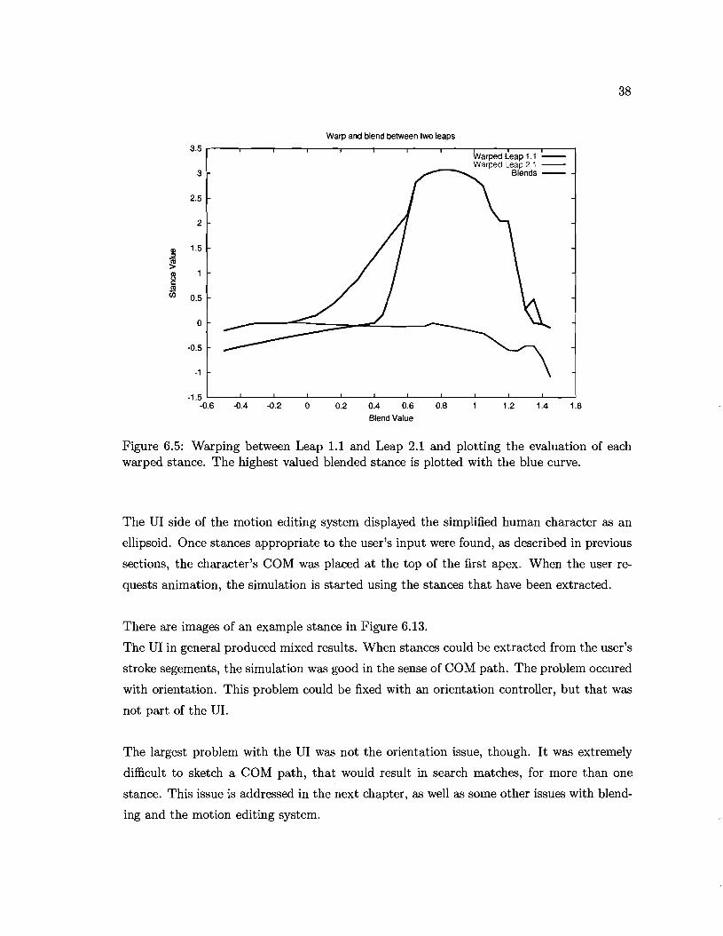
two stances, as was used in the previous blend figures could be used again. In Figures 6.5

and 6.6, each stance is warped to a state space location between each other, and the eval­

uation of that warped stance is plotted. Blends were created for each warped pair, using

35

COM paths

1.3 Leap 1.1 •Leap 2.1 lC

33% Blend 66% Blend

• 1.2 •

1.1

c 0 E Ul 0 a. Cii .2 t:: 0.9Q)

>

0.8

0.7

0.6 0 0.2 0.4 0.6 0.8 1.2

Heading Position

Figure 6.2: The COM paths for Leap 1.1, Leap 2.1, and two blends

blend values in increments of 0.1, i.e. 9 intermediate blends. Note that in some regions

along each of these plots, the blended stance is a dramatic improvement over the results

obtained by warping the individual stances.

The 50% blend that appeared questionable in Figure 6.3 can now be seen at the "Blend

Value" of 0.5 in Figure 6.6. Because the in this latest figure the value of the best blended

stance is being plotted, it is clear that the blend in Figure 6.3 is no better than ~ -0.5.

That means the blended Leap 1.1 and Run 0 stance from earlier is not physically plausible.

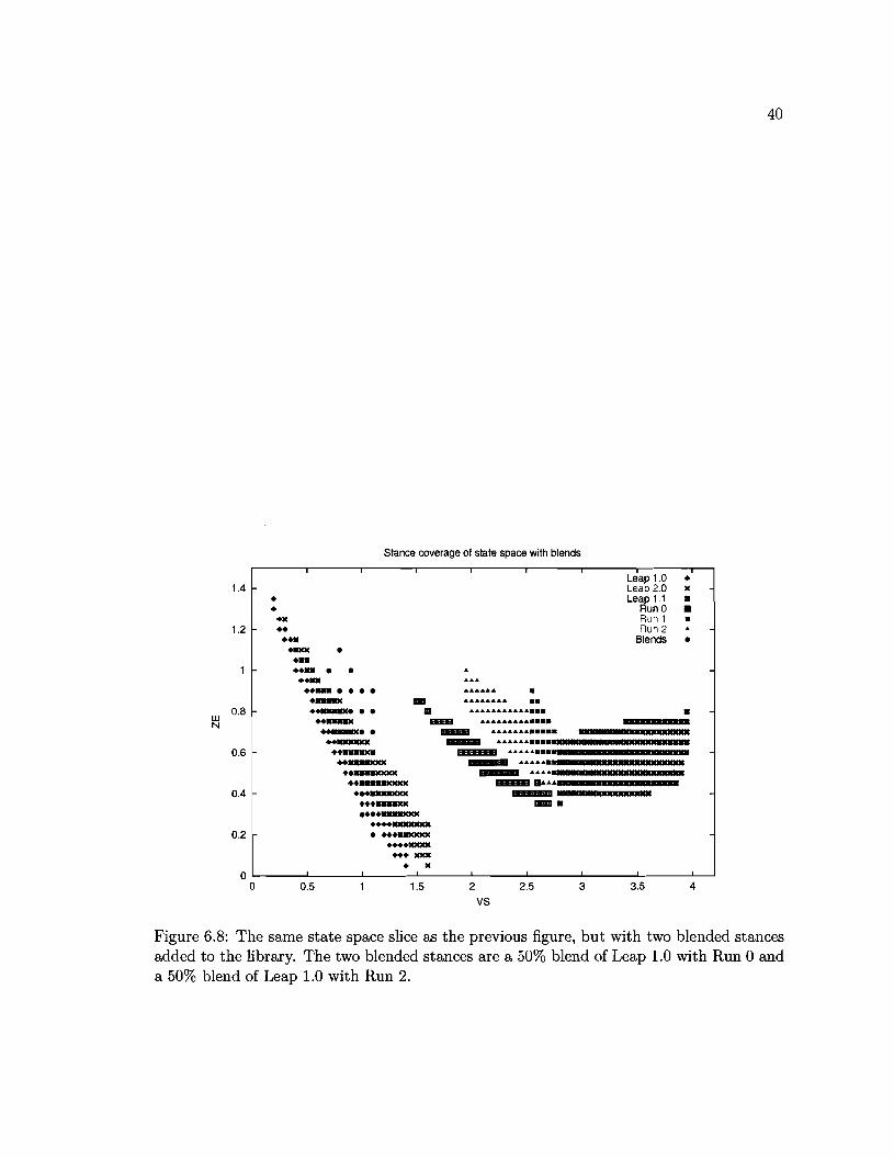
The major goal of blending was to fill in gaps in the state space. Figure 6.7 shows a slice

of state space that involves only warped stances and no blends. Now, with some evidence,

we could claim that blending makes a difference in the library's state space coverage. For

an example of blending filling in a previously vacant area, look to Figure 6.5. Each blend

value in this plot represents a unique point in the state space. It shows that neither original

stance can be effectively warped to the blend value 0.2, but that there are blends of the

stances that are effective at 0.2. For the best proof of this claim, see Figure 6.8.

Figure 6.8 is the same as Figure 6.7 except that there were two blended stances added to

36

COM paths

1.25 • II

Leap 1.0 Run 0

50% Blend -1.2

1.15

1.1c: 0 :~ 0 n, 1.05 ~ .€ CD >

0.95

0.9

0.85 -0.4 -0.2 0 0.2 0.4 0.6 0.8 1.2 1.4 1.6

Heading Position

Figure 6.3: The COM paths for Leap 1.0, Run 0, and a blend

the library. The stances were a 50% blend of Leap 1.0 with Run 0 and a 50% blend of

Leap 1.0 with Run 2. In Figure 6.3 the %50 blend of Leap 1.0 and Run 0 looked like it was

totally useless, but now it's obvious that that is not the case. Apparently it was useless

with those specific stance parameters, but useful when warped elsewhere in the state space.

6.2 Motion Editing System

The motion editing system consisted of a front-end, sketch-based interface, and a back-end,

search algorithm. When the animator sketched a COM path and its shadow, the VI would

extract from it the desired state space parameters. These desired parameters were then

fed to a search, which would use warping and blending to find matching, physically plausi­

ble stances. To guarantee plausibility, stance evaluation was used as the metric in the search.

The search algorithm first examines warped stances only, then tries taking the few best

stances and computing many blends. Finally, it tries blending all of the stances in the

library, using only a few blend values. The search met with mixed results in experiments

(done offline from the VI).

37

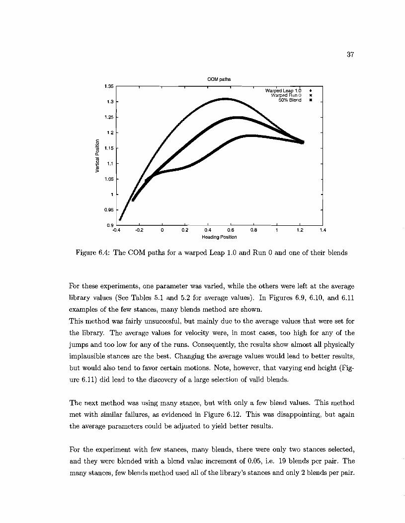
1.35 r----r----r---__r--­

1.3

1.25

1.2

c: .2 ''liS 1.15 ~

~ :e 1.1

~

1.05

0.95

50% Blend

COM paths __r---__r---__r----r----r-------,

Warped Leap 1.0 • Warped Run 0 x

-

0.9 L...-__L..-__L..-__L-__L...-__L...-__L..-__L..-__L..-_-----.J

-0.4 -0.2 o 0.2 0.4 0.6 0.8 1.2 1.4 Heading Position

Figure 6.4: The COM paths for a warped Leap 1.0 and Run 0 and one of their blends

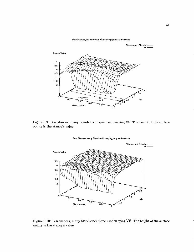
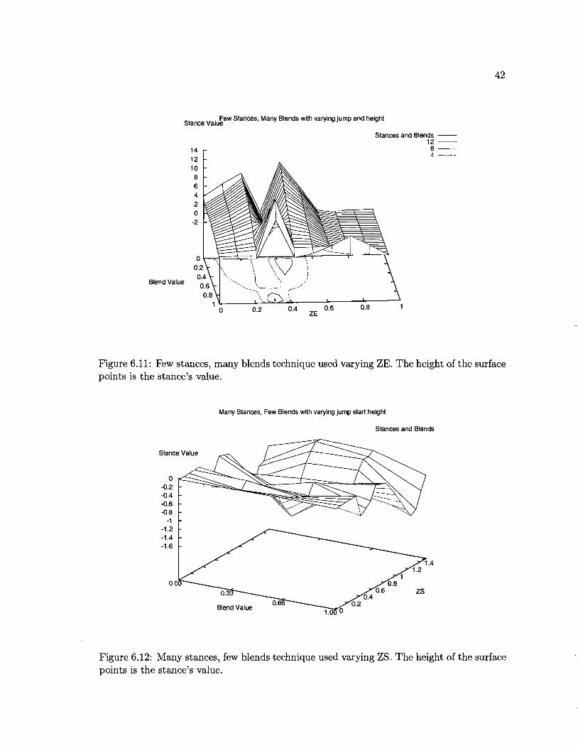
For these experiments, one parameter was varied, while the others were left at the average

library values (See Tables 5.1 and 5.2 for average values). In Figures 6.9, 6.10, and 6.11

examples of the few stances, many blends method are shown.

This method was fairly unsuccesful, but mainly due to the average values that were set for

the library. The average values for velocity were, in most cases, too high for any of the

jumps and too low for any of the runs. Consequently, the results show almost all physically

implausible stances are the best. Changing the average values would lead to better results,

but would also tend to favor certain motions. Note, however, that varying end height (Fig­

ure 6.11) did lead to the discovery of a large selection of valid blends.

The next method was using many stance, but with only a few blend values. This method

met with similar failures, as evidenced in Figure 6.12. This was disappointing, but again

the average parameters could be adjusted to yield better results.

For the experiment with few stances, many blends, there were only two stances selected,

and they were blended with a blend value increment of 0.05, i.e. 19 blends per pair. The

many stances, few blends method used all of the library's stances and only 2 blends per pair.

38

Warp and blend between two leaps

-1.5 '--_-'-_---'__-'-_---L__-'--_---'-__..I---_--'-__.l...-_-'-_---'

-0.6 -0.4 -0.2 o 0.2 0.4 0.6 0.8 1.2 1.4 1.6

Blend Value

Figure 6.5: Warping between Leap 1.1 and Leap 2.1 and plotting the evaluation of each warped stance. The highest valued blended stance is plotted with the blue curve.

The VI side of the motion editing system displayed the simplified human character as an

ellipsoid. Once stances appropriate to the user's input were found, as described in previous

sections, the character's COM was placed at the top of the first apex. When the user re­

quests animation, the simulation is started using the stances that have been extracted.

There are images of an example stance in Figure 6.13.

The VI in general produced mixed results. When stances could be extracted from the user's

stroke segements, the simulation was good in the sense of COM path. The problem occured

with orientation. This problem could be fixed with an orientation controller, but that was

not part of the VI.

The largest problem with the VI was not the orientation issue, though. It was extremely

difficult to sketch a COM path, that would result in search matches, for more than one

stance. This issue is addressed in the next chapter, as well as some other issues with blend­

ing and the motion editing system.

3.5 .-----.-----,r-----.-----,---r-----r--..------,---..-----,----, Warped Leap 1.1 -­Warped Leap 2.1 -­

Blends -­3

2.5

2

1.5

0.5

o

-0.5

-1

39

COM paths

0.5 Warped Leap 1.0 - ­

Warped Run 0 - ­Blends - ­

o

-0.5

-1

-1.5

-2 '-------'---_-'-'-_----'--l..._......._.....,Ij~_....L..._ ___l_ ___I......L..__f-L..L---l.-----J

-0.6 -0.4 -0.2 o 0.2 0.4 0.6 0.8 1.2 1.4 1.6 Blend Value

Figure 6.6: Warping between Leap 1.0 and run 0 and plotting the evaluation of each warped stance. The highest valued blended stance is plotted with the blue curve.

Stance coverage of state space

Leap 1.0 + 1.4 Leap 2.0 x

+ Leap 1.1 )l( + Run 0 D

+x Run1 • 1.2 ++ Run 2

++)l( +::tEXX

+** ++**

++** ++*** •

+ltE.1**X 00 •• ++****x )I(D....................0.8

UJ ++****X E:EER::J )IOIE:ll{)I(:ll{)1OI00010101EN ++****x ODDDD *.)I(~)I()I(*~**)IOIE.)I( ..)I(

++****xx DDDDDD *****.**.****** ~.

++****xx DDDDDDD **.**.******..~..~

++****xxx OODDDDD 0.6

*)I()I(**)I()IOIE.~***~)I(.)I(~)I(

++****xxxx DDOOOOD **.***********~**~*

++*****xxxx DDDDDD ~ *••**.****-**~**~.

0.4 +++****XXX DDDDDDD *•••******••••*** +++***It:XX DOD *

+++****xxx ++++ltEtntfXXXX

+++"B.~XXXX0.2 ++++xxxx

+++ xxx + x

0 40 0.5 1.5 2 2.5 3 3.5

VS

Figure 6.7: Valid stances are shown with points in this 2D slice of state space. Average library values were used for parameters other than VS and ZE.

••

40

1.4

1.2

0.8 w N

0.6

0.4

0.2

a

Stance coverage of state space with blends

Leap 1.0 •Leap 2.0 I(

Leap 1.1 Run a

.1( Run 1 ••••• Run 2 ••• Blends •

• MXX •... ..... . .... ..- .... •.- .. .. ••......-x••• • AAA••••••••••• ..

••-......-x. • --mmmmB •••••••••••• ~• • ..- mmmmmm ••••••••••

mmmmmBI ••••••••..­___ ......... ..10. .....~

...- .. ..10...10. ....­ _..... • •••••• ''CM...~ ........•••-.:JC)C

••••.-xJOC ••••IIIIII)C:J()O(

••••IIIDOOOC ••••)C)()Q(

••• xxx • I(

a 0.5 1.5 2 2.5 3 3.5 4

VS

Figure 6.8: The same state space slice as the previous figure, but with two blended stances added to the library. The two blended stances are a 50% blend of Leap 1.0 with Run 0 and a 50% blend of Leap 1.0 with Run 2.

41

Few Stances, Many Blends with varying jump start velocity

Stances and Blends -­0-­

Stance Value

1

0.5

o -0.5

-1

-1.5

-2

Figure 6.9: Few stances, many blends technique used varying VS. The height of the surface points is the stance's value.

Few Stances, Many Blends with varying jump end velocity

Stances and Blends -­0-­

Stance Value

0.5

o -0.5

-1

-1.5

-2

3

VE

Blend Value

Figure 6.10: Few stances, many blends technique used varying VE. The height of the surface points is the stance's value.

42

Stance valU~ew Stances, Many Blends with varying jump end height

Stances and Blends -­12 -­

14

12

8-­4 --­

10 8 6 4 2 o

-2

Blend Value

0.2 0.4o ZE

Figure 6.11: Few stances, many blends technique used varying ZE. The height of the surface points is the stance's value.

Many Stances, Few Blends with varying jump start height

Stances and Blends -­

Stance Value

o -0.2 -0.4 -0.6 -0.8

-1 -1.2 -1.4 -1.6

1.0 0

Figure 6.12: Many stances, few blends technique used varying ZS. The height of the surface points is the stance's value.

43

Figure 6.13: Screen shots from a stance simulation in the UI. The topmost image is the scene with screen arcs drawn. The remaining images are the simulation sequence for a stance and run across and down from the top left.

Chapter 7

Discussion and Future Work

The paper described a method for blending physically-based motion, and a user interface

that could utilize that method. There were various design issues that were dealt with in

both blending and the VI, including support polygon blending, the search algorithm, stance

parameter editing, and 3D curve editing. Chapters 4 and 5 explain the approaches that

were used to deal with those issues, but in the next two sections, alternative approaches are

discussed. Directions for future work are also mentioned.

7.1 Blending

The blending technique was fast and produced expected results, but there were some de­

cisions that could have been made differently. For instance the support polygon sequence

blending was done by choosing the sequence from the stance with the majority of contribu­

tion in the blend. That method does not involve blending the polygons at all though. This

was physically motivated. By choosing a valid support polygon from one of the motions, we

were guaranteed to have a valid combination of heel, foot, and toe contact at each timestep.

A geometric blend of the polygons, however, would have produced a smoother change of

behavior over the blend interval.

The general idea behind geometric blending of the polygon sequences is to first time-scale

the sequences to align the polygon timing. Then take each pair of polygons and blend them

as shown in Figure 7.1.

Most of the future work with this blending technique lies in improving the speed of the

44

45

a.

B

b.

Figure 7.1: a) Polygons A and B are positioned to allign one point from each, represented by the large dot. b) Lines are projected from the alligned points through each of the other points of both polygons, and represented by dashed lines where they are not the same as a side of either polygon. The red and blue points represent the intersection of the lines with polygons A and B respectively. Interpolation is done between corresponding red and blue points to create the blended polygon, which is drawn in green.

automated blending process that was described in Section 5.3. The simple search algorithm

that was used could not find solutions fast enough when a user desired more than a couple

of stances. More intelligent search techniques and/or library preprocessing steps would in­

crease the search speed tremendously.

The way the search works is to check the validity of the warped stances first, then start

computing and evaluating blends if none were satisfactory. The first blending technique

was to take just m, where m is small but m 2: 0, of the best matched, warped stances and

blend them with many different blend values. In this case, the best matched stances are

the ones that evaluated the highest. Chapter 3 defines stances as lying on a point in the

state space of stance parameters. The algorithm could choose the m best stance pairs for

blending by connecting each pair of state space points with a line and determining which

lines come nearest to the desired state space coordinate.

Vast improvements could also be possible with effective preprocessing of the library's stances.

46

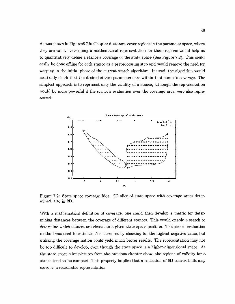
As was shown in Figures6.7 in Chapter 6, stances cover regions in the parameter space, where

they are valid. Developing a mathematical representation for these regions would help us

to quantitatively define a stance's coverage of the state space (See Figure 7.2). This could

easily be done offline for each stance as a preprocessing step and would remove the need for

warping in the initial phase of the current search algorithm. Instead, the algorithm would

need only check that the desired stance parameters are within that stance's coverage. The

simplest approach is to represent only the validity of a stance, although the representation

would be more powerful if the stance's evaluation over the coverage area were also repre­

sented.

lE I

I),~

o,~

f.1,1

tl..B

D.'

D.q

D.]

lU i.s t

Figure 7.2: State space coverage idea. 2D slice of state space with coverage areas deter­mined, also in 2D.

With a mathematical definition of coverage, one could then develop a metric for deter­

mining distances between the coverage of different stances. This would enable a search to

determine which stances are closest to a given state space position. The stance evaluation

method was used to estimate this closeness by checking for the highest negative value, but

utilizing the coverage notion could yield much better results. The representation may not

be too difficult to develop, even though the state space is a higher-dimensional space. As

the state space slice pictures from the previous chapter show, the regions of validity for a

stance tend to be compact. This property implies that a collection of 6D convex hulls may

serve as a reasonable representation.

47

7.2 User Interface

The motion editing system was developed to permit straightforward and interactive use of

the warping and blending algorithms. It was, however, designed and implemented as a proof

of concept more than a polished system. So there are some areas that were not perfected,

and even some issues that were not dealt with at all.

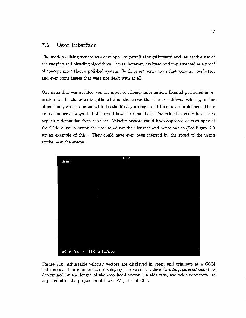
One issue that was avoided was the input of velocity information. Desired positional infor­

mation for the character is gathered from the curves that the user draws. Velocity, on the

other hand, was just assumed to be the library average, and thus not user-defined. There

are a number of ways that this could have been handled. The velocities could have been

explicitly demanded from the user. Velocity vectors could have appeared at each apex of

the COM curve allowing the user to adjust their lengths and hence values (See Figure 7.3

for an example of this). They could have even been inferred by the speed of the user's

stroke near the apexes.

Figure 7.3: Adjustable velocity vectors are displayed in green and originate at a COM path apex. The numbers are displaying the velocity values (heading / perpendicular) as determined by the length of the associated vector. In this case, the velocity vectors are adjusted after the projection of the COM path into 3D.

48

The first method would defeat the purpose of using a mouse for easy input. Requiring the

user to stop intermediately to use the keyboard would only serve to frustrate the user and

slow his/her production. The second method is preferable to the first, because it is much

more intuitive. Here the user doesn't have to deal directly with numbers, but rather with

lengths of vectors, which are easily compared and edited on the screen. Finally, inferring

velocity from the speed of the COM stroke would prevent cluttering the screen with data,

but would force the user to control the mouse position and speed fairly precisely. Because

the only way to edit any portions or characteristics of a curve is to delete the curve and

start over, the user would have far too much trouble using this method.

Another feature that would have been useful is general editing of the parabolic stance curves.

There are some techniques that have been developed for this. Work done by J. Cohen, et

al [4] allowed the user to overdraw strokes or portions of strokes. Their algorithm would

blend the overdrawn stroke with the already drawn 3D curve.

It was easy to draw a curve for which stances could not be matched. This was due in part to

the lack of a scale. The user had no way to know what size the obstacles in the environment

were, making it a laborious task to sketch an acceptable curve.

Because the library of motions was small and there was a lack of any scale references, most

sketched curves had multiple segments that were matched by no stances. When there is

no match, the user should be informed. It is not clear, however, exactly how this feedback

should be provided to the user. The system currently has no technique for determining,

or even guessing, which of the desired stance parameters is/are preventing the search from

finding an answer. The animator is required to use intuition, which works fine for a fairly

small motion library, but fails for a large one.

Different problems occur in situations where some curve segments are fitted with stances,

but others are not. Editing a segment (remember that this lies between two consecutive

apexes) of the COM curve will effect the neighboring curve segments. That effect will in

turn force the VI to search for new stances for the edited curve segment as well as the

neighboring segments. While this sequence of events is logical, it will frustrate users to fix

the effected segments that were previously fine.

The blending algorithm is solid and could easily be worked into a motion editing system.

49

More work is required for a search that uses blending, and that work should focus on

gaining a better understanding of the state space. While the VI did serve its purpose as a

proof-of-concept, much more work is needed to address the issues that I mentioned above.

Bibliography

[1] Ascension Technology Corp. Manufacturer of motion capture technology,

http://www.ascension-tech.com.

[2] D. Baraff. Fast contact force computation for nonpenetrating rigid bodies. In Computer

Graphics (SIGGRAPH '94 Proceedings), July 1994.

[3] A. Bruderlin and L. Williams. Motion signal processing. In Computer Graphics (SIG­

GRAPH '95 Proceedings), pages 97-104, August 1995.

[4] J. M. Cohen, L. Markosian, R. Zeleznik, J. F. Hughes, R. Barzel. An interface for

sketching 3D curves. In Symposium on Interactive 3D Graphics, 1999.

[5] M. F. Cohen. Interactive spacetime control for animation. In Computer Graphics (SIG­

GRAPH '92 Proceedings), volume 26, pages 293-302, July 1992.

[6] T. H. Cormen, C. E. Leiserson, and R. L. Rivest. Introduction to Algorithms. MIT

Press, 1990.

[7] M. Gleicher. Motion editing with spacetime constraints. In M. cohen and D. Zeltzer, ed­

itors, 1997 Symposium on Interactive 3D Graphics, pages 139-148. ACM SIGGRAPH,

April 1997. ISBN 0-89791-884-3.

[8] M. Gleicher. Retargetting Motion to New Characters. In Computer Graphics (SIG­

GRAPH '98 Proceedings), pages 33-42, July 1998.

[9] M. Gleicher and P. Litwinowicz. Constraint-based motion adaptation. The Journal of

Visualization and Computer Animation, 9(2):65-94, 1998.

[10] J. K. Hodgins and N. S. Pollard. Adapting simulated behaviors for new characters. In

Computer Graphics (SIGGRAPH '97 Proceedings), pages 153-162, 1997.

50

51

[11] J. K. Hodgins, W. Wooten, D. Brogan, J. F. O'Brien. Animating human athletics. In

Computer Graphics (SIGGRAPH '95 Proceedings), pages 71-78, 1995.

[12] InterSense, Inc. Manufacturer of motion capture technology, http://www.isehse.com.

[13] A. Lamouret and M. van de Panne. Motion synthesis by example. Computer Animation

and Simulation '96 - Proceedings of the 7th Eurographics Workshop on Simulation

and Animation, Springer Verlag. Poitiers, France, August 31 - September 1, 1996,

pages 199-212.

[14] J. Lee and S. Y. Shin. A hierarchical approach to interactive motion editing for human­

like figures. In Computer Graphics (SIGGRAPH '99 Proceedings), 1999.

[15] Z. Liu, S. J. Gortler, and M. F. Cohen. Hierarchical spacetime control. In Computer

Graphics (SIGGRAPH '94 Proceedings), July 1994.

[16] N. S. Pollard and F. Behmaram-Mosavat. Interactive, Force-Based Motion Editing for

Locomotion Tasks. In Proceedings of the IEEE International Conference on Robotics

and Automation, San Francisco, CA, April 2000.

[17] Z. Popovic and A. Witkin. Physically based motion transformation. SIGGRAPH 1999

Proceedings, Aug. 1999.

[18] M. H. Raibert and J. K. Hodgins. Animation of dynamic legged locomotion. In Com­

puter Graphics (SIGGRAPH '91 Proceedings), volume 25, pages 349-358, July 1991.

[19] C. Rose, M. F. Cohen, and B. Bodenheimer. Verbs and Adverbs: Multidimensional

motion interpolation. IEEE Computer Graphics & Applications, 18(5), September ­

October 1998.

[20] C. Rose, B. Guenter, B. Bodenheimer, and M. Cohen. Efficient generation of motion

transitions using spacetime constraints. In Computer Graphics (SIGGRAPH '96 Pro­

ceedings), pages 147-154, 1996.

[21] M. Unuma, K. Anjyo, and R. Takeuchi. Fourier principles for emotional-based human

figure animation. In Computer Graphics (SIGGRAPH '95 Proceedings), 1995.

[22] M. van de Panne. From footprints to animation. Computer Graphics Forum, 16(4):211­

224,1997.

52

[23] A. Witkin and M. Kass. Spacetime constraints. In Computer Graphics (SIGGRAPH

'88 Proceedings), volume 22, pages 159-168, August 1988.

[24] A. Witkin and Z. Popovic. Motion warping. In Computer Graphics (SIGGRAPH '95

Proceedings), August 1995.

[25] R. Zeleznik, K. Herndon, and J. F. Hughes. Sketch: An interface for sketching 3d

scenes. In Computer Graphics (SIGGRAPH '96 Proceedings), August 1996.

[26] J. Zhao and N. Badler. Inverse kinematics positioning using nonlinear programming

for highly articulated figures. In ACM Transactions on Graphics 13(4) pp. 313-336,

October 1994.