Embed Size (px)
Citation preview
Motion estimation from image and inertialmeasurements
Dennis W. Strelow
November 2004CMU-CS-04-178
School of Computer ScienceCarnegie Mellon University
Pittsburgh, PA 15213
Thesis Committee:Dr. Sanjiv Singh, chair
Dr. Martial HebertDr. Michael Lewicki
Dr. Rama Chellappa, University of Maryland
Submitted in partial fulfillment of the requirementsfor the degree of Doctor of Philosophy
© 2004 Dennis W. Strelow
All rights reserved
This research was sponsored by Exponent, Inc. under a US Army contract, Athena Technologies under USAir Force grant number F08630-03-0024, Allied Aerospace Industries under Army Procurement Office contractnumber MDA972-01-9-0017, a NASA Graduate Student Researchers Program (GSRP) fellowship under grantnumber NGT5-50347, and the Honda Motor Company. The views and conclusions contained in this documentare those of the author and should not be interpreted as representing the official policies, either expressed orimplied, of any sponsoring institution, the U.S. government or any other entity.

Keywords: batch shape-from-motion, recursive shape-from-motion, inertialnavigation, omnidirectional vision, sensor fusion, long-term motion estimation
Abstract
Robust motion estimation from image measurements would be an enabling technology forMars rover, micro air vehicle, and search and rescue robot navigation; modeling complexenvironments from video; and other applications. While algorithms exist for estimating sixdegree of freedom motion from image measurements, motion from image measurementssuffers from inherent problems. These include sensitivity to incorrect or insufficient imagefeature tracking; sensitivity to camera modeling and calibration errors; and long-term driftin scenarios with missing observations, i.e., where image features enter and leave the fieldof view.
The integration of image and inertial measurements is an attractive solution to some ofthese problems. Among other advantages, adding inertial measurements to image-basedmotion estimation can reduce the sensitivity to incorrect image feature tracking and cam-era modeling errors. On the other hand, image measurements can be exploited to reducethe drift that results from integrating noisy inertial measurements, and allows the addi-tional unknowns needed to interpret inertial measurements, such as the gravity directionand magnitude, to be estimated.
This work has developed both batch and recursive algorithms for estimating cameramotion, sparse scene structure, and other unknowns from image, gyro, and accelerome-ter measurements. A large suite of experiments uses these algorithms to investigate theaccuracy, convergence, and sensitivity of motion from image and inertial measurements.Among other results, these experiments show that the correct sensor motion can be recov-ered even in some cases where estimates from image or inertial estimates alone are grosslywrong, and explore the relative advantages of image and inertial measurements and ofomnidirectional images for motion estimation.
To eliminate gross errors and reduce drift in motion estimates from real image se-quences, this work has also developed a new robust image feature tracker that exploitsthe rigid scene assumption and eliminates the heuristics required by previous trackers forhandling large motions, detecting mistracking, and extracting features. A proof of conceptsystem is also presented that exploits this tracker to estimate six degree of freedom motionfrom long image sequences, and limits drift in the estimates by recognizing previouslyvisited locations.

Acknowledgments
I want to thank my advisor, Sanjiv Singh, for hundreds of hours of research discussionsand encouragement; and for listening to, carefully reading, and suggesting improvementsin many talks and papers, including this document. I also want to thank Sanjiv for hispersonal and career advice, which has benefited me very much.
My thanks also go to Martial Hebert, Mike Lewicki, and Rama Chellappa, for agreeingto serve on my committee, and making time for me alongside their students. Their differ-ent viewpoints, careful reading, and veteran advice have been very helpful.
I also want to thank Jeff Mishler, for what has now been almost eight years of valuableand direct advice, and for lucidly explaining why gasoline and ammunition are the cur-rency of the future. Similarly, I am indebted to Henele Adams for his expert advice. Mythanks go to Tom Minka for immediately reading, and for adeptly finding and correctly aproblem in, an earlier version of this work.
Many people helped in capturing the data used in my experiments, including HeneleAdams, Dan Bartz, Mark Delouis, Ivan Kirigin, Matt Mason, Jeff Mishler, Wenfan Shi, JimTeza, Chris Urmson, Michael Wagner, and David Wettergreen, among others.
v

Contents
1 Introduction 11.1 Motion estimation . . . . . . . . . . . . . . . . . . . . . . . . . . . . . . . . . . 1
1.2 Motion estimation from image measurements . . . . . . . . . . . . . . . . . . 3
1.3 Robust motion estimation from image measurements . . . . . . . . . . . . . 5
1.3.1 Motion estimation from omnidirectional image measurements . . . . 6
1.3.2 Motion estimation from image and inertial measurements . . . . . . 6
1.3.3 Constrained image feature tracking . . . . . . . . . . . . . . . . . . . 7
1.3.4 Long-term motion estimation . . . . . . . . . . . . . . . . . . . . . . . 7
1.4 Organization . . . . . . . . . . . . . . . . . . . . . . . . . . . . . . . . . . . . . 8
2 Related work and background 92.1 Omnidirectional vision . . . . . . . . . . . . . . . . . . . . . . . . . . . . . . . 9
2.2 Batch motion estimation from image and inertial measurements . . . . . . . 10
2.3 Recursive motion estimation from image and inertial measurements . . . . 11
2.4 SLAM and shape-from-motion . . . . . . . . . . . . . . . . . . . . . . . . . . 14
2.5 Data association and image feature tracking . . . . . . . . . . . . . . . . . . . 15
2.6 Sparse image feature tracking . . . . . . . . . . . . . . . . . . . . . . . . . . . 16
2.7 Shape-from-motion with missing observations . . . . . . . . . . . . . . . . . 18
2.8 Long-term image-based motion estimation . . . . . . . . . . . . . . . . . . . 20
2.9 Background: conventional camera projection models and intrinsics . . . . . 21
2.10 Background: bundle adjustment . . . . . . . . . . . . . . . . . . . . . . . . . 23
3 Motion from noncentral omnidirectional image sequences 273.1 Overview . . . . . . . . . . . . . . . . . . . . . . . . . . . . . . . . . . . . . . . 27
3.2 Omnidirectional cameras . . . . . . . . . . . . . . . . . . . . . . . . . . . . . . 28
3.3 Computing omnidirectional projections . . . . . . . . . . . . . . . . . . . . . 31
3.4 Omnidirectional camera calibration . . . . . . . . . . . . . . . . . . . . . . . 34
vii
viii CONTENTS
3.5 Experimental results . . . . . . . . . . . . . . . . . . . . . . . . . . . . . . . . 36
3.5.1 Overview . . . . . . . . . . . . . . . . . . . . . . . . . . . . . . . . . . 36
3.5.2 Correctness of the estimated parameters . . . . . . . . . . . . . . . . 37
3.5.3 Effect of calibration on estimated motion and structure . . . . . . . . 38
3.6 Discussion . . . . . . . . . . . . . . . . . . . . . . . . . . . . . . . . . . . . . . 39
4 Motion from image and inertial measurements: algorithms 414.1 Overview . . . . . . . . . . . . . . . . . . . . . . . . . . . . . . . . . . . . . . . 41
4.2 Motion from image or inertial measurements alone . . . . . . . . . . . . . . 42
4.3 Batch algorithm . . . . . . . . . . . . . . . . . . . . . . . . . . . . . . . . . . . 43
4.3.1 Overview . . . . . . . . . . . . . . . . . . . . . . . . . . . . . . . . . . 43
4.3.2 Inertial error . . . . . . . . . . . . . . . . . . . . . . . . . . . . . . . . . 45
4.3.3 Accelerometer bias prior error . . . . . . . . . . . . . . . . . . . . . . 47
4.3.4 Minimization . . . . . . . . . . . . . . . . . . . . . . . . . . . . . . . . 47
4.3.5 Discussion . . . . . . . . . . . . . . . . . . . . . . . . . . . . . . . . . . 48
4.4 Recursive estimation . . . . . . . . . . . . . . . . . . . . . . . . . . . . . . . . 49
4.4.1 Overview . . . . . . . . . . . . . . . . . . . . . . . . . . . . . . . . . . 49
4.4.2 State vector and initialization . . . . . . . . . . . . . . . . . . . . . . . 50
4.4.3 State propagation . . . . . . . . . . . . . . . . . . . . . . . . . . . . . . 50
4.4.4 Measurement updates . . . . . . . . . . . . . . . . . . . . . . . . . . . 51
4.4.5 Newly acquired points . . . . . . . . . . . . . . . . . . . . . . . . . . . 52
4.4.6 Lost points . . . . . . . . . . . . . . . . . . . . . . . . . . . . . . . . . . 56
4.4.7 Image-only estimation . . . . . . . . . . . . . . . . . . . . . . . . . . . 56
4.4.8 Discussion . . . . . . . . . . . . . . . . . . . . . . . . . . . . . . . . . . 57
5 Motion from image and inertial measurements: experiments 595.1 Overview . . . . . . . . . . . . . . . . . . . . . . . . . . . . . . . . . . . . . . . 59
5.2 Experiments overview . . . . . . . . . . . . . . . . . . . . . . . . . . . . . . . 60
5.2.1 The experiments . . . . . . . . . . . . . . . . . . . . . . . . . . . . . . 60
5.2.2 Inertial sensors . . . . . . . . . . . . . . . . . . . . . . . . . . . . . . . 60
5.2.3 Motion error metrics . . . . . . . . . . . . . . . . . . . . . . . . . . . . 62
5.3 Perspective arm experiment . . . . . . . . . . . . . . . . . . . . . . . . . . . . 63
5.3.1 Camera configuration . . . . . . . . . . . . . . . . . . . . . . . . . . . 64
5.3.2 Observations . . . . . . . . . . . . . . . . . . . . . . . . . . . . . . . . 64
5.3.3 Batch image-and-inertial estimates . . . . . . . . . . . . . . . . . . . . 64
5.3.4 Batch image-only estimates . . . . . . . . . . . . . . . . . . . . . . . . 70
CONTENTS ix
5.3.5 Recursive image-and-inertial estimates . . . . . . . . . . . . . . . . . 735.3.6 Covariance estimates . . . . . . . . . . . . . . . . . . . . . . . . . . . . 775.3.7 Summary . . . . . . . . . . . . . . . . . . . . . . . . . . . . . . . . . . 78
5.4 Omnidirectional arm experiments . . . . . . . . . . . . . . . . . . . . . . . . 805.4.1 Sensor configuration . . . . . . . . . . . . . . . . . . . . . . . . . . . . 805.4.2 Observations . . . . . . . . . . . . . . . . . . . . . . . . . . . . . . . . 815.4.3 Batch image-and-inertial estimates . . . . . . . . . . . . . . . . . . . . 835.4.4 Batch image-only estimates . . . . . . . . . . . . . . . . . . . . . . . . 845.4.5 Recursive image-and-inertial estimates . . . . . . . . . . . . . . . . . 845.4.6 Summary . . . . . . . . . . . . . . . . . . . . . . . . . . . . . . . . . . 84
5.5 Perspective crane experiment . . . . . . . . . . . . . . . . . . . . . . . . . . . 875.5.1 Camera configuration . . . . . . . . . . . . . . . . . . . . . . . . . . . 875.5.2 Observations . . . . . . . . . . . . . . . . . . . . . . . . . . . . . . . . 875.5.3 Estimate . . . . . . . . . . . . . . . . . . . . . . . . . . . . . . . . . . . 89
5.6 Perspective rover experiment . . . . . . . . . . . . . . . . . . . . . . . . . . . 895.6.1 Camera configuration . . . . . . . . . . . . . . . . . . . . . . . . . . . 905.6.2 Observations . . . . . . . . . . . . . . . . . . . . . . . . . . . . . . . . 905.6.3 Recursive image-only estimates . . . . . . . . . . . . . . . . . . . . . . 915.6.4 Recursive image-and-inertial algorithm . . . . . . . . . . . . . . . . . 935.6.5 Discussion . . . . . . . . . . . . . . . . . . . . . . . . . . . . . . . . . . 95
6 Robust feature tracking for motion estimation 976.1 Overview . . . . . . . . . . . . . . . . . . . . . . . . . . . . . . . . . . . . . . . 976.2 Lucas-Kanade . . . . . . . . . . . . . . . . . . . . . . . . . . . . . . . . . . . . 996.3 Lucas-Kanade and real sequences . . . . . . . . . . . . . . . . . . . . . . . . . 1026.4 Background: epipolar geometry and the fundamental matrix . . . . . . . . . 1036.5 Tracker design and implementation . . . . . . . . . . . . . . . . . . . . . . . 105
6.5.1 Overview . . . . . . . . . . . . . . . . . . . . . . . . . . . . . . . . . . 1056.5.2 Epipolar geometry estimation . . . . . . . . . . . . . . . . . . . . . . . 1056.5.3 Epipolar search . . . . . . . . . . . . . . . . . . . . . . . . . . . . . . . 1126.5.4 Geometric mistracking detection . . . . . . . . . . . . . . . . . . . . . 1136.5.5 Feature thinning and extraction . . . . . . . . . . . . . . . . . . . . . . 113
6.6 Results Overview . . . . . . . . . . . . . . . . . . . . . . . . . . . . . . . . . . 1146.7 Evaluation methodology . . . . . . . . . . . . . . . . . . . . . . . . . . . . . . 116
6.7.1 Feature fates . . . . . . . . . . . . . . . . . . . . . . . . . . . . . . . . . 1176.7.2 Estimating correct feature positions . . . . . . . . . . . . . . . . . . . 117
x CONTENTS
6.7.3 Identifying grossly mistracked features . . . . . . . . . . . . . . . . . 1186.7.4 Drift estimates . . . . . . . . . . . . . . . . . . . . . . . . . . . . . . . 118
6.8 Evaluation . . . . . . . . . . . . . . . . . . . . . . . . . . . . . . . . . . . . . . 1186.9 Future directions . . . . . . . . . . . . . . . . . . . . . . . . . . . . . . . . . . 120
7 Long-term motion estimation 1237.1 Overview . . . . . . . . . . . . . . . . . . . . . . . . . . . . . . . . . . . . . . . 1237.2 Method . . . . . . . . . . . . . . . . . . . . . . . . . . . . . . . . . . . . . . . . 124
7.2.1 Active state . . . . . . . . . . . . . . . . . . . . . . . . . . . . . . . . . 1247.2.2 Rollback states . . . . . . . . . . . . . . . . . . . . . . . . . . . . . . . 1257.2.3 Extending states . . . . . . . . . . . . . . . . . . . . . . . . . . . . . . 1257.2.4 Operation . . . . . . . . . . . . . . . . . . . . . . . . . . . . . . . . . . 1267.2.5 Example . . . . . . . . . . . . . . . . . . . . . . . . . . . . . . . . . . . 127
7.3 Results . . . . . . . . . . . . . . . . . . . . . . . . . . . . . . . . . . . . . . . . 1297.3.1 Overview . . . . . . . . . . . . . . . . . . . . . . . . . . . . . . . . . . 1297.3.2 Input sequence . . . . . . . . . . . . . . . . . . . . . . . . . . . . . . . 1297.3.3 System parameters . . . . . . . . . . . . . . . . . . . . . . . . . . . . . 1317.3.4 Estimates . . . . . . . . . . . . . . . . . . . . . . . . . . . . . . . . . . 134
7.4 Discussion . . . . . . . . . . . . . . . . . . . . . . . . . . . . . . . . . . . . . . 134
8 Conclusion 1418.1 Overview . . . . . . . . . . . . . . . . . . . . . . . . . . . . . . . . . . . . . . . 1418.2 Conclusions . . . . . . . . . . . . . . . . . . . . . . . . . . . . . . . . . . . . . 1418.3 Recommendations . . . . . . . . . . . . . . . . . . . . . . . . . . . . . . . . . 1438.4 Contributions . . . . . . . . . . . . . . . . . . . . . . . . . . . . . . . . . . . . 1448.5 Future directions . . . . . . . . . . . . . . . . . . . . . . . . . . . . . . . . . . 146
List of Figures
2.1 The perspective and orthographic projection models . . . . . . . . . . . . . . 22
3.1 Single viewpoint and noncentral omnidirectional projection models . . . . . 293.2 Example scene points and their equiangular omnidirectional projections . . 303.3 The adjustable equiangular camera rig and an example image . . . . . . . . 303.4 The rigid equiangular camera and an example image . . . . . . . . . . . . . 313.5 The constraints that determine the mirror reflection point for a given scene
point . . . . . . . . . . . . . . . . . . . . . . . . . . . . . . . . . . . . . . . . . 333.6 Equiangular projections resulting from misalignment between the conven-
tional camera and mirror . . . . . . . . . . . . . . . . . . . . . . . . . . . . . . 353.7 The known points and calibration images used in the omnidirectional cam-
era calibration experiments . . . . . . . . . . . . . . . . . . . . . . . . . . . . 40
4.1 The batch and recursive algorithms for estimating motion from image andinertial measurements . . . . . . . . . . . . . . . . . . . . . . . . . . . . . . . 44
5.1 The organization of the experiments . . . . . . . . . . . . . . . . . . . . . . . 615.2 Example images from the perspective arm experiment . . . . . . . . . . . . . 655.3 The translation estimates generated by the batch image and inertial algo-
rithm for the perspective arm experiment . . . . . . . . . . . . . . . . . . . . 665.4 The average and maximum translation errors from Table 5.1, shown as a
function of the inertial error function variances . . . . . . . . . . . . . . . . . 695.5 Estimates for the perspective arm experiment generated using the batch
image-only method . . . . . . . . . . . . . . . . . . . . . . . . . . . . . . . . . 715.6 The average translation errors given in Table 5.5 for the recursive image-
and-inertial algorithm, as a function of the linear acceleration and angularvelocity propagation variances . . . . . . . . . . . . . . . . . . . . . . . . . . 76
5.7 Translation covariances estimates for the perspective arm sequence . . . . . 79
xi
xii LIST OF FIGURES
5.8 Examples images from the first omnidirectional camera experiment . . . . . 81
5.9 Example images from the second omnidirectional experiment . . . . . . . . 82
5.10 The x, y translation estimates generated by the batch image-and-inertial andbatch image-only algorithms for the first and second omnidirectional armexperiments . . . . . . . . . . . . . . . . . . . . . . . . . . . . . . . . . . . . . 86
5.11 Example images from the perspective crane experiment . . . . . . . . . . . . 88
5.12 The x, y translation estimate for the perspective crane experiment generatedby the recursive image-and-inertial method . . . . . . . . . . . . . . . . . . . 89
5.13 The z translation estimates for perspective crane experiment generated bythe recursive image-and-inertial method . . . . . . . . . . . . . . . . . . . . . 90
5.14 An example image from the perspective rover sequence showing differentfeature densities . . . . . . . . . . . . . . . . . . . . . . . . . . . . . . . . . . . 91
5.15 Example images from the perspective rover sequence showing feature track-ing through the sequence . . . . . . . . . . . . . . . . . . . . . . . . . . . . . . 92
5.16 Estimates and ground truth values for the x, y translation in the perspectiverover experiment . . . . . . . . . . . . . . . . . . . . . . . . . . . . . . . . . . 94
6.1 Features tracked across 20 images of the classic “hotel” sequence . . . . . . 101
6.2 The distribution of tracking errors for the “hotel” subsequence . . . . . . . . 101
6.3 The epipolar geometry relating two images . . . . . . . . . . . . . . . . . . . 104
6.4 An overview of the tracker design . . . . . . . . . . . . . . . . . . . . . . . . 106
6.5 SIFT keypoint extraction . . . . . . . . . . . . . . . . . . . . . . . . . . . . . . 107
6.6 Randomly subsampled SIFT matches . . . . . . . . . . . . . . . . . . . . . . . 109
6.7 Images corrected for radial and tangential distortion . . . . . . . . . . . . . . 110
6.8 Example features and their epipolar lines . . . . . . . . . . . . . . . . . . . . 111
7.1 The structure of the proof of concept system states . . . . . . . . . . . . . . . 125
7.2 The initial operation of the system. . . . . . . . . . . . . . . . . . . . . . . . . 127
7.3 A new position and covariance are found during normal, non-rollback op-eration . . . . . . . . . . . . . . . . . . . . . . . . . . . . . . . . . . . . . . . . 128
7.4 A new position and covariance are found by extending a rollback state . . . 128
7.5 A rollback state is extended and adopted as the new active state . . . . . . . 129
7.6 Several states that result from extending a rollback state have been adoptedas the active state . . . . . . . . . . . . . . . . . . . . . . . . . . . . . . . . . . 130
7.7 Eight representative images from the first forward pass in the full “highbay”sequence . . . . . . . . . . . . . . . . . . . . . . . . . . . . . . . . . . . . . . . 132

LIST OF FIGURES xiii
7.8 Two estimates of the “highbay” camera motion and sparse scene structureduring the first forward pass . . . . . . . . . . . . . . . . . . . . . . . . . . . 133
7.9 Reacquisition image pairs . . . . . . . . . . . . . . . . . . . . . . . . . . . . . 1367.10 Areas for which the system loses the position estimate . . . . . . . . . . . . . 137


List of Tables
3.1 The average reprojection errors for each sequence and calibration in the cal-ibration experiments . . . . . . . . . . . . . . . . . . . . . . . . . . . . . . . . 37
3.2 The estimated rotations for each of the full calibrations . . . . . . . . . . . . 38
3.3 The estimated translations for each of the full calibrations . . . . . . . . . . . 38
3.4 The mirror apex locations for each of the calibrations . . . . . . . . . . . . . 39
3.5 The reprojection and range errors for each sequence and calibration in thecalibration experiments . . . . . . . . . . . . . . . . . . . . . . . . . . . . . . . 39
5.1 The error metrics and iterations required for convergence for the Set A esti-mates from the perspective arm experiment . . . . . . . . . . . . . . . . . . . 68
5.2 The error metrics and iterations required for convergence for the Set B esti-mates from the perspective arm experiment . . . . . . . . . . . . . . . . . . . 71
5.3 The camera intrinsics estimates and standard deviations for the perspectivearm experiment . . . . . . . . . . . . . . . . . . . . . . . . . . . . . . . . . . . 72
5.4 The sensitivity of image-only batch estimation to camera intrinsics calibra-tion errors and to image observation errors . . . . . . . . . . . . . . . . . . . 73
5.5 The average error metrics for the Set A estimates generated using the recur-sive image-and-inertial algorithm . . . . . . . . . . . . . . . . . . . . . . . . . 75
5.6 The error metrics for the Set B estimates generated using the recursive image-and-inertial algorithm . . . . . . . . . . . . . . . . . . . . . . . . . . . . . . . 76
5.7 The error metrics for the Set C estimates generated using the recursive image-and-inertial algorithm . . . . . . . . . . . . . . . . . . . . . . . . . . . . . . . 77
5.8 The error metrics for the first, second, and third omnidirectional arm exper-iments . . . . . . . . . . . . . . . . . . . . . . . . . . . . . . . . . . . . . . . . 85
6.1 The characteristics of the test image sequences . . . . . . . . . . . . . . . . . 116
xv
xvi LIST OF TABLES
6.2 The fates of features tracked in the test sequences, and statistics describinghow long features were tracked in the sequence . . . . . . . . . . . . . . . . 119
6.3 Percentages of grossly mistracked points for the test sequences . . . . . . . . 1196.4 Tracking error and drift rate statistics for drifting features tracked in the test
sequences . . . . . . . . . . . . . . . . . . . . . . . . . . . . . . . . . . . . . . 1206.5 Average/maximum tracking errors for the synthetic symmetric sequences . 121
7.1 The system’s reacquisition behavior for the two experiments . . . . . . . . . 135
Chapter 1
Introduction
1.1 Motion estimation
Robust, long-term motion estimation would be an enabling technology for many problemsin autonomous robotics and modeling from video. For example:
• Mars rovers must visit objects of interest that human operators identify in the rover’sview. However, the long communications latency between earth and Mars and longperiods without communications limit the frequency with which the rover’s oper-ators can send commands. So, the rovers are most productive if they can performthese traverses autonomously. Accurate on-board estimation of the rover’s motion isan important component in performing these traverses successfully.
• Astronauts on the International Space Station sometimes perform dozens of exper-iments a day, spanning many disciplines. NASA Ames Research Center has beendeveloping a softball-sized Personal Satellite Assistant (PSA)[4][3] that can movearound the station in six degrees of freedom to maximize the astronaut’s produc-tivity during these experiments and monitor conditions on the station. For example,the PSA would allow experts on earth to move around the station and collaborate inexperiments virtually, via the PSA’s cameras; would provide a hands-free terminalfor astronauts performing delicate experiments; and would monitor conditions inconfined locations inaccessible to the astronauts. Each of these capabilities requiresthat the PSA be able to estimate its position on the station, accurately and over thelong-term.
• Micro air vehicles (MAVs) are under development that can be launched from theground, and carry a video camera and chemical sensors for surveillance, search and
1
2 Chapter 1. Introduction
rescue, air sampling, and other applications. AeroVironment’s Black Widow[24], forinstance, has a wingspan of 6 inches, a mass of less than 100 grams, a maximumcommunications range of 2 kilometers, and an endurance of 30 minutes, making it agood candidate for discrete surveillance over the horizon, around the corner in theurban canyon, or under the canopy in wooded areas. However, to report the locationof activity or chemical threats, the vehicle’s position must be accurately estimated.
• Recent search and rescue robot designs are capable of moving over highly uneventerrain, into spaces deep within rubble. To report the location of survivors, theserobots should estimate their position in six degrees of freedom.
• Modeling complex environments like building interiors and cities from image se-quences is a long-standing problem in computer vision research (for example, see El-Hakim[13]). If the camera’s motion can be accurately established, then the problemreduces to modeling the geometry and surface properties of objects in the environ-ment from images taken at known locations.
Each of the following is required by some or all of these example problems.
• Six degree of freedom motion. Motion estimation for the Personal Satellite Assis-tant, micro air vehicles, and modeling complex environments are inherently six de-gree of freedom problems. Mars rovers and search and rescue robots are groundvehicles but may move over nonplanar terrain, so their motion is best modeled us-ing six degrees of freedom.
• Motion in unknown environments. Mars rovers, micro air vehicles, search and res-cue robots, and modeling complex environments must all operate in unknown envi-ronments. While the International Space Station is a partially known environment, itis subject to change as components are moved around the station, and known fidu-cials are not welcome on the station.
• Motion over the long term. All of the examples require estimation over the longterm.
• Motion from small, light, and inexpensive sensors. The Personal Satellite Assistantrequires small and light sensors. Micro air vehicles require small, light, and cheapsensors, since ideal micro air vehicles are disposable.
• Motion without GPS or other absolute position systems. GPS is not available onMars or on the International Space Station, and other systems that might be used for
1.2. Motion estimation from image measurements 3
absolute positioning, such as known fiducials or beacons, are not suitable for use onthe station. Micro air vehicles and search and rescue robots may enter environments,such as building interiors or rubble, respectively, where GPS cannot be received;and MAVs’ access to GPS can be jammed. While systems for modeling complexenvironments can use GPS outdoors, GPS is not useful for modeling interiors.
Many common sensors are poor candidates given these requirements. Odometry is notsuitable for six degree of freedom estimation. Range devices are often large, heavy, andexpensive; and are limited in range. Inertial sensors alone are not suitable for motionestimation over the long-term, because integrating their measurements produces drift inthe estimated motion.
However, cameras are good candidates for each of these problems. Cameras can beused to estimate six degree of freedom motion in unknown environments, without GPSand over the long term, as described in the next section. Cameras can be made small, lightand cheap. Furthermore, cameras are not inherently limited in range and do not emit anyenergy into the environment.
1.2 Motion estimation from image measurements
As mentioned in the previous section, cameras are good candidates for six degree of free-dom motion estimation, and many methods exist for extracting motion from images. Oneparadigm splits the problem into two steps:
1. Extract and track sparse image features through the image sequence.
2. Estimate the six degree of freedom camera position at the time of each image.
The first step, feature extraction and tracking, establishes the image locations (“projec-tions”) of points in the scene from different vantage points. This step is normally per-formed with one of two approaches, called template matching and feature extraction andmatching in subsequent sections. Sections 2.5 and 2.6 below discuss sparse feature trackingand these two approaches, respectively, in more detail. Chapter 6 describes a new trackerthat, among other qualities, combines the best of these two approaches.
Many algorithms exist for the second step, estimation, with different advantages anddisadvantages. Some existing algorithms for the estimation step figure prominently in thefollowing chapters:
1. Bundle adjustment[61][57] uses general nonlinear minimization to simultaneouslyfind the six degree of freedom camera position at the time of each image, and the
4 Chapter 1. Introduction
three-dimensional point positions, that maximize the likelihood of the observed track-ing data. Bundle adjustment is a batch method, meaning that all of the observa-tions are required before the computation begins; is iterative, so an initial estimate ofthe camera and point positions are required; and can be computationally expensive.However, bundle adjustment naturally accommodates arbitrary camera models andmissing observations (i.e., the case where features enter and leave the field of view),and is usually considered the gold standard algorithm. Bundle adjustment is re-viewed below in Section 2.10.
2. The iterated extended Kalman filter (IEKF)[16] can be used to estimate the same un-knowns and minimize roughly the same function as bundle adjustment[5], but in arecursive fashion that processes tracked features from each image as they arrive. Mo-tion estimation using Kalman filtering can be performed in real-time, but as Chapters4 and 5 below explain, Kalman filtering for motion estimation is problematic in thecase of missing observations, and suffers from poor a priori assumptions on the cam-era motion.
3. The variable state dimension filter (VSDF)[38] is a recursive method that combinesaspects of bundle adjustment and Kalman filtering. Like Kalman filtering algo-rithms for motion estimation, the VSDF estimates the same unknowns and mini-mizes roughly the same error function as bundle adjustment. However, the VSDFis explicitly designed to handle the case of missing observations within a recursiveframework, and jettisons the assumptions on camera motion that hamper Kalmanfilter algorithms. On the other hand, the VSDF has difficulties handling featuresleaving and then reentering the image sequence.
4. Two- and three-frame methods for shape-from-motion solve for the camera motionbetween pairs and triples, respectively, of images in the sequence, and concatenatethe two- and three-frame motions to produce an estimate of the overall (“multi-frame”) motion[26]. These methods can be efficient, but they are ad hoc in thatthey do not produce or approximate the optimal estimate of the overall motion. Thetracker described in Chapter 6 below uses two- and three-frame estimation in thecontext of sparse image feature tracking.
Algorithms 1, 2, and 3 are shape-from-motion algorithms, meaning that they simultane-ously estimate both shape (the three-dimensional point positions) and motion (the six de-gree of freedom camera positions). The two- and three-frame methods are also sometimes
1.3. Robust motion estimation from image measurements 5
referred to as shape-from-motion algorithms, even though the two- and three-frame mo-tions can be found without simultaneously finding the shape.
The algorithms in subsequent chapters are based on these shape-from-motion algo-rithms, but in this work the term “shape-from-motion” is usually deprecated in favor of“motion estimation” for two reasons. First, “shape-from-motion” implies that the goal is torecover shape, with the motion recovered as a necessary intermediate quantity, whereas inour applications the situation is exactly the opposite. Second, “shape-from-motion” refersto algorithms that recover motion from image measurements, whereas much of the em-phasis in subsequent chapters is on motion from both image and inertial measurements.
In addition to the problems listed above for each estimation algorithm, motion estima-tion from images suffers from some long-standing difficulties. Estimation generally suffersfrom:
• sensitivity to incorrect or insufficient image feature tracking
• sensitivity to camera modeling and calibration errors
• sensitivity to outlier detection thresholds
• sensitivity to degenerate camera motions
• long-term drift in scenarios with missing observations, due to all of the above
• ambiguities, such as depth reversal, in the shape and motion estimates
In addition, batch algorithms such as bundle adjustment suffer from:
• the need for an initial estimate, and poor convergence or failure to converge if theinitial estimate is poor
• poor convergence or failure to converge if the percentage of missing observations ishigh
and recursive algorithms suffer from:
• poor approximations in modeling the state prior distribution
• poor assumptions about the camera motion, e.g., smoothness
1.3 Robust motion estimation from image measurements
This thesis investigates some strategically chosen approaches to some of these problems.
6 Chapter 1. Introduction
1.3.1 Motion estimation from omnidirectional image measurements
Motion from omnidirectional images is a promising approach for removing many of thesensitivities that cause gross location errors in motion estimates, including sensitivity toincorrect feature tracking, sensitivity to outlier thresholds, and ambiguities. In addition,because features may be visible through more of an omnidirectional image sequence, om-nidirectional images may significantly reduce drift in long image sequences.
Chapter 3 below explores motion estimation from omnidirectional images. An omnidi-rectional projection model is developed for use with existing motion estimation algorithmssuch as bundle adjustment and Kalman filtering, which accommodates the wide designspace of noncentral omnidirectional cameras and misalignment between the camera andmirror. A calibration algorithm is described for determining the misalignment, and the ef-fect of omnidirectional images and this precise calibration on motion estimation accuracyare examined.
1.3.2 Motion estimation from image and inertial measurements
Image and inertial measurements are highly complimentary modalities for motion estima-tion. As mentioned in Section 1.1, inertial measurements alone are not appropriate for mo-tion estimation, because random errors, unmodeled nonlinearities, and slowly changingbiases in inertial measurements cause the motion estimates to drift. With image measure-ments, however, this drift can be minimized and other unknowns needed to interpret theinertial measurements, such as the gravity direction and magnitude, can be estimated. Onthe other hand, inertial measurements can help to reduce the sensitivity of image-only mo-tion estimation to feature tracking errors and camera calibration errors, and establish theglobal scale of the motion, which cannot be recovered from image measurements alone.
Chapter 4 describes both batch and recursive algorithms for estimating sensor motion,sparse scene structure, and other unknowns from image, gyro, and accelerometer mea-surements. These algorithms are designed to recover accurate estimates of the unknowns,if possible, even when the estimates from image or inertial measurements alone may begrossly wrong. Chapter 5 uses these algorithms and a large suite of experiments to ex-plore the relative sensitivity of image-only and image-and-inertial motion estimation, therelative advantages of image-and-inertial estimation and estimation from omnidirectionalimages, and many other issues.

1.3. Robust motion estimation from image measurements 7
1.3.3 Constrained image feature tracking
As mentioned above, motion estimation can be sensitive to incorrect or insufficient featuretracking. Poor tracking can result from:
• large image motions
• unmodeled changes in features’ appearance between images, resulting from lightingchanges, specularities, occlusions, or foreshortening
• insufficient, repetitive, or one-dimensional image texture
• poor spatial distribution of features in the image
The long-time go-to feature tracker in the shape-from-motion community, Lucas-Kanade,is susceptible to all of these problems. The work presented in this thesis has developed anew tracker that exploits SIFT keypoints[36] to establish the epipolar geometry betweenimages, constrains tracking between images to one dimension, and eliminates Lucas-Kanade’sheuristics for handling large motions, detecting mistracking, and extracting features. Theresulting tracker qualitatively outperforms Lucas-Kanade on many real sequences, and isdescribed in detail in Chapter 6, along with experimental results.
1.3.4 Long-term motion estimation
Motion estimates from image sequences with high percentages of missing observations,such as those taken from a moving vehicle, contain drift. While this drift can be reducedby carefully addressing the issues described in Section 1.2 above, drift cannot be eliminatedcompletely because the sensors’ position is not being estimated relative to a single, alwaysvisible external landmark.
If the camera repeatedly moves between locations in a bounded area, however, it shouldbe possible to limit drift by:
1. recognizing when a previously mapped area has been revisited
2. using new observations of the revisited area to limit drift in the estimates
While the second problem has been widely explored in the simultaneous localization andmapping literature in the context of ground rovers with range scanners and odometry, thefirst problem is unique to image-based motion estimation. Chapter 7 describes a proof ofconcept system that exploits the tracker described in Chapter 6, the variable state dimen-sion filter, and SIFT keypoints to demonstrate limited drift.

8 Chapter 1. Introduction
1.4 Organization
The organization of this document is as follows. Chapter 2 reviews related work andpresents the background material that is common to the subsequent chapters. Chapters3-7 investigate the avenues of approach described in Section 1.3 above:
• Chapter 3 describes motion estimation from omnidirectional images.
• Chapters 4 and 5 describe algorithms and experimental results for motion estimationfrom image and inertial measurements, respectively.
• Chapter 6 describes the new image feature tracker.
• Chapter 7 describes long-term motion estimation.
Chapter 8 concludes by recapping the conclusions and contributions of the work, givingsome explicit recommendations, and describing possible future directions.

Chapter 2
Related work and background
As described in the introduction, this work investigates a number of approaches to improv-ing motion estimation from image measurements. Sections 2.1-2.8 in this chapter reviewprevious work related to these approaches. In addition, Sections 2.9 and 2.10 review con-ventional camera projection models and bundle adjustment, respectively, which are usedextensively in subsequent chapters.
2.1 Omnidirectional vision
Recent omnidirectional camera designs include catadioptric designs, which combine aconventional camera with a mirror that expands the camera’s field of view. During thelast few years, researchers have been active in the design, modeling, and calibration ofthese cameras, and in exploiting these cameras for motion estimation and localization. Asthe overview in Chapter 3 explains, the wide field of view provided by these cameras ispromising for improving the robustness and accuracy motion estimation from images.
The recent widespread interest in catadioptric cameras in the computer vision commu-nity was sparked by Nayar’s design[41], which combines an orthographic camera with aparabolic mirror. This design achieves a single viewpoint, i.e., rays that are reflected fromthe mirror into the conventional camera’s center also intersect at a single point inside themirror. This single viewpoint property allows portions of the omnidirectional image tobe correctly remapped to perspective views, and the viewpoint inside the mirror can beadopted as the camera’s center for the purpose of defining the camera’s epipolar geome-try. The entire class of single viewpoint catadioptric designs was explored by Baker andNayar[1].
The definitive study of single viewpoint cameras for three-dimensional computer vi-
9
10 Chapter 2. Related work and background
sion is given in a sequence of papers by Geyer and Daniilidis, who emphasize Nayar’s de-sign. Their investigation includes modeling[17], epipolar geometry[22], calibration[20][17],rectification[21], projective geometry[18], and uncalibrated structure and motion[19] forthese cameras.
Other work on single viewpoint camera calibration includes Kang[35], who describestwo methods for single viewpoint camera calibration. The first recovers the image centerand mirror parabolic parameter from the image of the mirror’s circular boundary in oneimage. The second method uses minimization to recover skew in addition to the othercalibration parameters. Other work on motion estimation with single viewpoint camerasincludes Gluckman and Nayer[23], who extend three algorithms for ego-motion estima-tion with conventional cameras to the single viewpoint case.
On the other hand, relatively little work has been done with non-single-viewpoint, ornoncentral, catadioptric cameras. Examples of noncentral catadioptric cameras includeChahl and Srinivasan’s design[8], which sacrifices the single viewpoint property to gainnearly uniform image resolution between the omnidirectional image’s center and periph-ery. Ollis’ design[46], which is used in this work, refines Chahl and Srinivasan’s designto achieve exactly uniform resolution between the image’s center and periphery. Singleviewpoint cameras where there is a known misalignment between the camera and mirrorlose their single viewpoint property, but can be modeled as noncentral cameras.
Chapter 3 below presents an omnidirectional camera model that accommodates non-central cameras and known misalignment between the camera and mirror; camera cal-ibration using this model; and camera motion estimation using this model. Chapter 5investigates the relative advantages of motion estimation from omnidirectional camerasand from conventional camera and inertial measurements.
2.2 Batch motion estimation from image and inertial measure-ments
Chapter 4 below describes batch and recursive methods for estimating sensor motion,sparse scene structure, and other unknowns from image, gyro, and accelerometer mea-surements. This section and the next briefly review the existing methods for estimatingsensor motion from image and inertial measurements that are most closely related to thesemethods. While the majority of existing methods are recursive, a few relevant batch meth-ods do exist, and both batch and recursive methods for this problem are reviewed, in thissection and in Section 2.3, respectively.
2.3. Recursive motion estimation from image and inertial measurements 11
Deans and Hebert[11] describe a batch method for bearings-only localization and map-ping that uses Levenberg-Marquardt to estimate the planar motion of a vehicle and thetwo-dimensional location of landmarks observed by the vehicle’s omnidirectional camera,from the landmarks’ vehicle coordinate system bearings (one-dimensional projections) andthe vehicle’s odometry. The error function described in Section 4.3, which utilizes image,gyro, and accelerometer measurements, is closely related to Deans and Herbert’s image-and-odometry error function. However, estimating six degree of freedom motion fromimage measurements and inertial sensors introduces some difficulties that do not arise inestimating planar motion from bearings and odometry. In particular, using image mea-surements for six degree of freedom motion normally requires careful modeling and cal-ibration of the camera, especially in the omnidirectional case, whereas this modeling isnot required in two dimensions. In addition, the use of accelerometer observations forsix degree of freedom motion requires estimation of the vehicle’s velocity and orienta-tion relative to gravity, which odometry does not require. In subsequent work[12], Deansalso considered iteratively reweighted least squares (IRLS) for robust estimation withinthe batch framework, to improve the quality of estimates in the presence of image featuremistracking and other gross observation errors.
A second batch method is described by Jung and Taylor[33]. This method appliesshape-from-motion to a set of widely spaced keyframes from an omnidirectional imagesequence, then interpolates the keyframe positions by a spline that best matches the in-ertial observations. The resulting algorithm provides a continuous estimate of the sen-sor motion, and only requires that feature correspondences be established between thekeyframes, rather than between every image in the sequence. Since the image and inertialmeasurements are not used simultaneously, however, the interpolation phase will propa-gate rather than fix errors in the motion estimated in the shape-from-motion phase.
2.3 Recursive motion estimation from image and inertial mea-surements
Huster and Rock[30][31][29][32] detail the development of a recursive algorithm for es-timating the six degree of freedom motion of an autonomous underwater vehicle (AUV)using gyro measurements, accelerometer measurements, and the image measurements of asingle point in the vehicle’s environment. In Huster and Rock[30], the authors develop anextended Kalman filter (EKF) and a two-step algorithm for a simplified, two-dimensionalversion of the motion estimation problem. The difficulties with linearizing the measure-
12 Chapter 2. Related work and background
ment equations about uncertain estimates in the EKF are sidestepped in the two-step filter,which chooses the state so that the image and inertial measurement equations become lin-ear, and avoids linearization in the state time propagation using the unscented filter. InHuster and Rock[29], a full three-dimensional version of the two-step filter is constructed,and integrated with a controller and a method for choosing an endpoint trajectory thatoptimizes the quality of the motion estimates. The authors’ experiments show that the re-sulting system reliably performs a grasping task on a manipulator. In the measurementsemployed and in the quantities estimated, this system has many similarities to the iter-ated extended Kalman filter (IEKF) for motion estimation described in Section 4.4, but ismore sophisticated in its handling of nonlinearities. However, the use of a single imagepoint feature, which is motivated by the potentially poor quality of underwater images,precludes the use of Huster and Rock’s method for long distance traverses.
You and Neumann[62] describe an augmented reality system for estimating a user’sview relative to known fiducials, using gyro and image measurements. This method issimpler than Huster and Rock’s in that it does not employ an accelerometer, which is amore difficult instrument to incorporate than a rate gyro, but expands the scene from asingle point to a set of known points. Rehbinder and Ghosh[52] also describe a systemfor estimating motion relative to a known scene, in this case containing three-dimensionallines rather than point features. Rehbinder and Ghosh incorporate accelerometer measure-ments as well as gyro and image measurements.
Qian, et al.[50] describe an extended Kalman filter (EKF) for simultaneously estimatingthe motion of a sensor rig and the sparse structure of the environment in which the rigmoves, from gyro and image measurements. The authors show motion estimation ben-efits from the addition of gyro measurements in several scenarios, including sequenceswith mistracking and “mixed domain” sequences containing both sensor translation andpure rotation. This system is more general than that described by Huster and Rock, Youand Neumann, or Rehbinder and Ghosh, in that the sparse scene structure is estimated inaddition to the motion rather than known, but this system makes the implicit assumptionthat each scene point is visible in every image of the sequence. In later work, Qian andChellappa[49] also investigated motion estimation from image and gyro measurementswithin a sequential Monte Carlo framework. In this case, the authors showed that the in-clusion of gyro measurements significantly reduced the number of samples required foraccurate motion estimation.
Chai, et al.[9] describe a system for simultaneously estimating the motion of a sensorrig and the sparse structure of the environment in which the rig moves, from gyro, ac-celerometer, and image measurements. This system estimates nearly the same unknowns
2.3. Recursive motion estimation from image and inertial measurements 13
as the algorithm described in Chapter 4, but divides the estimation task between a mo-tion filter, which estimates motion by assuming that the scene structure is known, and astructure filter, which estimates the scene structure by assuming the motion is known. Thetwo filters are combined into a system for simultaneous estimation of motion and scenestructure by supplying the estimates from each filter as the known inputs to the other.While this arrangement improves efficiency, it will result in artificially low covarianceson the estimated motion and structure, particularly for long-term problems where due todrift, the motion and the scene structure are likely to contain large but coupled errors. Theauthors do not explicitly consider the problem of estimating motion in sequences wherepoints enter and leave the image sequence. The authors also consider the relative benefitsof using one and two cameras in synthetic tests, and conclude that the use of two camerascan produce estimates with significantly lower errors.
The system described by Mukai and Ohnishi[40] also simultaneously estimates the mo-tion of a sensor rig and the sparse structure of the environment in which the rig movesusing gyro and image measurements. In Mukai and Ohnishi’s method, the motion be-tween pairs of images is estimated up to a scale factor, and the estimated motion is usedto determine the structure of the points seen in both images. These pairwise estimates arethen merged sequentially by applying the scaled rigid transformation that best aligns therecovered structures. This method handles sequences where points do not appear in everyimage, but both the pairwise motion recovery and merging steps of this method are adhoc. For instance, this method does not maintain any measure of the error in the resultingmotion estimates.
Foxlin[15] describes a general framework for recursive simultaneous localization, map-ping, and sensor calibration. The system consists of a decentralized filter that integratesthe results of three complimentary error filters for localization only, localization and map-ping, and localization and sensor calibration. This architecture reduces the computationrelative to including environmental object locations and sensor calibration parameters inthe same state vector, and allows mapping and sensor calibration to be easily removedfrom the estimation once the positions of environmental objects or sensor bias values havebeen estimated with sufficient accuracy. In [14], the authors describe one instance of thisarchitecture, which uses gyro measurements, accelerometer measurements, and the imagemeasurements of fiducials whose appearance but not (in general) location are known. Inthe case of auto-mapping, where the locations of fiducials are not known, the system poseis first determined relative to four fiducials whose x, y, z positions are known, and thepositions of subsequently acquired fiducials are entered into the filter using the image lo-cation and distance to the fiducial estimated from the fiducial’s image size. In the system
14 Chapter 2. Related work and background
described here, the initial position is initialized without a priori knowledge of any featurelocations using a batch algorithm, and the positions of natural features are initialized us-ing triangulation from multiple image positions, which is more appropriate for featureswhose appearance is not known a priori. While the authors report real-time performancefor an initial implementation of automapping, they do not report on the accuracy of theirsystem for automapping.
In addition to the batch algorithm described in Section 2.2, Deans[12] describes a hy-brid batch-recursive method that estimates the planar motion of a vehicle and the two-dimensional location of landmarks observed by the vehicle’s omnidirectional camera fromthe landmarks’ vehicle coordinate system bearings (one-dimensional projections) and thevehicle’s odometry. This method adapts the variable state dimension filter (VSDF), orig-inally described by McLauchlan[38] for shape-from-motion, to recursively minimize thesame image-and-odometry error function minimized by Deans and Hebert’s batch method.This approach naturally handles cases where points enter and leave the image sequence,and delays the linearization of measurements until the estimates used in the linearizationare more certain, reducing bias in the state estimate prior. A similar adaptation of thebatch algorithm for estimating motion from image and inertial measurements describedhere, using the VSDF, would be a natural extension of this work.
2.4 SLAM and shape-from-motion
Simultaneous localization and mapping (SLAM) and shape-from-motion (SFM) are twobroad areas concerned with simultaneously estimating sensor motion and scene structure.This section briefly contrasts these problems and discusses their relevance for long-termimage-based motion estimation. This section does not describe specific methods for SLAMand shape-from-motion. Instead, see Deans[12] for a good overview of specific methodsfor these problems.
Algorithms for simultaneous localization and mapping (SLAM) typically estimate pla-nar vehicle motion and the two-dimensional positions of landmarks in the vehicle’s envi-ronment using observations from the vehicle’s odometry and from a device that providesboth the range and bearing to the landmarks. Since both range and bearing are available,the device provides noisy two-dimensional landmark positions in the device’s coordinatesystem, and the major technical problem becomes the correct incorporation of these vehiclesystem measurements into the global coordinate system mean and covariance estimates.Recent work on SLAM focuses on mapping large areas, in which each landmark may onlybe visible from a small portion of the vehicle path, in a recursive fashion; and on “closing
2.5. Data association and image feature tracking 15
the loop”, which exploits a landmark that has been lost and reacquired to maintain thetopological consistency of the reconstructed motion and landmark positions.
Algorithms for shape-from-motion typically estimate the six degree of freedom motionof a camera and the three-dimensional position of points, from point features tracked inthe camera’s image sequence. Here, the observations the camera provides are the two-dimensional projections of landmark positions in the camera’s coordinate system, ratherthan the three-dimensional camera system position, so in SLAM terminology, one wouldsay that the camera provides bearings but not range. So, shape-from-motion typicallyestimates more unknowns than SLAM from less generous data. However, very little workhas been done on automatically mapping large areas or on closing the loop using recursiveshape-from-motion.
The motion estimation algorithms in Chapter 5 estimate six degree of freedom motion,sparse scene structure, and other unknowns from image, gyro, and accelerometer mea-surements. So, they fall somewhere between SLAM and shape-from-motion in terms of theobservations and recovered unknowns. In terms of the technical approach, the algorithmsdescribed in Chapter 5 are more akin to existing algorithms for SFM than to approaches forSLAM. This bias toward shape-from-motion is also reflected in the work on long-term mo-tion estimation in Chapter 7, and future algorithms would benefit from SLAM approachesto estimating errors and closing the loop within a recursive framework.
2.5 Data association and image feature tracking
In many scenarios where multiple targets are tracked over time using radar, sonar, or sim-ilar sensors, the correspondence between the targets and the measurements they generateat any one time is required for tracking the targets, but is not given explicitly. The problemof matching measurements with the tracked targets that generated them is called data as-sociation. Because the measurements alone may provide no information about which tar-get generated them, methods for data association typically associate measurements with atarget based on the likelihood of the measurements given the target’s estimated kinemat-ics. So, the problems of target tracking and data association become coupled. In scenarioswhere the targets may cross each other, may maneuver erratically, and may not produce ameasurement at each time, elaborate data associate algorithms may be necessary. A goodreview of these issues and the corresponding approaches for tracking and data associationis given by Bar-Shalom and Li[2].
The data association paradigm has been widely adopted in SLAM for associating sonaror laser returns with the landmarks in the environment that generated them. Montemerlo
16 Chapter 2. Related work and background
and Thrun’s approach[39] is a recent example. In the computer vision community, the dataassociation paradigm has been investigated for image feature tracking by Rasmussen andHager[51]. In this case, the authors applied two baseline data association methods, theprobabilistic data association filter (PDAF) and joint probabilistic data association filter(JPDAF), to the problems of tracking homogeneous colored regions, textured regions, andnonrigid image contours.
In shape-from-motion and image-based motion estimation, the targets and measure-ments are three-dimensional points and their image projections, respectively. There aretwo major differences between this scenario and traditional data association applicationslike associating radar returns with the target that generated them. First, the image ap-pearance in the neighborhood of each projection provides strong identifying informationabout the tracked point. Second, the scene is assumed rigid, so that targets are not movingindependently. As a result, there is less motivation for using kinematics in image featuretracking than in traditional data association problems.
There are two variations on the image feature tracking problem. In the first, a largenumber of features, typically 50-200, must be tracked between adjacent images in videoso that the camera motion relative to recent times can be estimated. For this problem,template matching or feature extraction and matching have often been used in the shape-from-motion literature, and these techniques are briefly reviewed in Section 2.6 below.
In the second variation, features that have left the camera’s view and later reentered,possibly at a much later time, should be recognized so that the camera’s position relative toa more distant time can be estimated. Using the estimated camera and point positions forthis purpose is promising, and would couple the estimation and matching just as track-ing and data association are coupled in other applications. Possible approaches for thisproblem are described in Section 2.8.
2.6 Sparse image feature tracking
Sparse feature tracking provides the image positions of three-dimensional points from dif-ferent vantage points that make shape-from-motion and motion estimation from imagespossible. Two paradigms for sparse feature tracking are common.
Template matching is the first paradigm. In this approach, a small intensity templateis extracted around the feature’s location in the current image, and the feature’s locationin the new image is found by minimizing the difference between the template intensitiesand the intensities around the location in the new image. The template sizes, the differ-ence metric, and the parameterization of the features’ locations in the new image vary. For
2.6. Sparse image feature tracking 17
example, the affine transformation of a 21 × 21 pixel template might be found that mini-mizes the sum-of-absolute-differences (SAD) between the template intensities and the newimage intensities.
The methods used to search for the minimizing location in the new image also vary. Abrute force approach computes the difference metric at discrete locations in the new im-age, within some rectangle around the feature’s location from the previous image. Lucas-Kanade is a more elegant approach, which uses iterative optimization to minimize thesum-of-squared-differences (SSD) between the template and new image intensities. Lucas-Kanade has long been the go-to tracker in the shape-from-motion community, but is notsufficient for demanding applications. Lucas-Kanade, its advantages, and its shortcomingsfor motion estimation are described in detail in Sections 6.2 and 6.3.
Independent extraction and matching is the second paradigm. In this approach, salientfeatures are extracted independently in the two images, and a consistent set of matchesbetween the two sets of features is found using a combinatorial search. Matched fea-tures are then linked across multiple images to produce feature tracking across multipleviews. Systems adopting this approach include DROID[25], which extracts Harris featuresin each image, and matches features between images based on the intensities in the fea-tures’ neighborhoods, geometry consistency, and the estimated camera kinematics. Nister,et al.[45] describe a real-time system for camera motion estimation that also extracts Harriscorners and matches them based on nearby intensities and geometric consistency. Thisalgorithm is described in more detail in Section 2.7 below, in the context of shape-from-motion with missing observations.
A disadvantage of independent extraction and matching is that it only tracks featuresas long as they are extracted in the new image. So, the average length of feature tracksis limited by the repeatability of extraction in the presence of feature appearance changes.For example, Harris reports roughly 80% repeatability for the Harris extractor[25]. So, wewould expect to see a feature in only several consecutive images before it is lost.
SIFT keypoints[36] are a recent development that can also be used for feature extractionand matching. SIFT keypoints are image locations that can reliably extracted to subpixelresolution under image transformations such as rotation, scaling, and affine or projectivetransformations. A SIFT feature vector associated with each keypoint describes the imageintensities near the keypoint in a way that is also nearly invariant to these transformations,providing a simple method for matching corresponding keypoints in two images withoutassumptions on the relative position (e.g., proximity) of the keypoints in the two images.
Chapter 6 below describes a new tracker that, among other qualities, combines theseparadigms. SIFT keypoints and their associated feature vectors are first used for feature
18 Chapter 2. Related work and background
extraction and matching, respectively. These matches are used to establish the epipolargeometry between adjacent images in the sequence. Discrete template matching and one-dimensional Lucas-Kanade are then used to find the rough position for features of intereston their epipolar lines in the new image, and to refine those positions, respectively. Thetracker’s use of independent extraction and matching and of template matching, are de-scribed in detail in subsections 6.5.2 and 6.5.3, respectively.
2.7 Shape-from-motion with missing observations
Shape-from-motion problems with missing observations, in which features become oc-cluded, enter and leave the field of view, or are lost due to mistracking, are a long-standingdifficulty in shape-from-motion. Among batch algorithms for shape-from-motion, bun-dle adjustment[61][55] and iterative versions[47] of the factorization method accommo-date missing observations. Among recursive algorithms, the variable state dimension fil-ter (VSDF) is explicitly designed to handle missing observations, and Section 4.4 belowconsiders missing observations in the iterated extended Kalman filter (IEKF) framework.Ad hoc algorithms that operate by sequentially concatenating 2-frame and 3-frame shape-from-motion solutions, which are discussed in more detail at the end of this section, natu-rally handle missing observations.
However, three issues remain:
1. If the percentage of missing observations is high, bundle adjustment and iterativefactorization algorithms will fail to converge, or converge much too slowly.
2. In features rapidly enter and leave the field of view, the camera’s position can nolonger be estimated with respect to a single, always visible external landmark. So,even small errors in feature tracking and camera intrinsics calibration necessarilylead to drift in the camera position estimates.
3. Features that leave and then reenter the field of view are problematic for recursivemethods, even in the case of the VSDF, which is explicitly designed to handle missingobservations.
Poelman’s[47] exploration of his iterative factorization algorithm’s convergence on syn-thetic datasets with varying percentages of missing observations and image observationnoise levels illustrates issue 1 above. He found that his method performed well for missingobservation percentages below some threshold, typically 50% for datasets with 2.0 pixel
2.7. Shape-from-motion with missing observations 19
image observation noise and 70% for datasets with 0.1 pixel image observation noise, andfailed “catastrophically” for datasets with higher percentages.
Weng, et al.[60] investigated 2 by deriving an analytical result describing the accuracyof optimal shape and motion estimates from image measurements as the percentage ofmissing observations varies. They show that for a scenario including some reasonablesimplifying assumptions, the error variance in both the estimated shape and motion in-creases as O(n/(f2)), where the n is the number of images and f is the average number ofimages that each point was visible in. That is, the error variances increase rapidly with thepercentage of missing observations.
Issue 3 has been largely ignored in the shape-from-motion community. But, the SLAMliterature is largely concerned with recursively estimation of a robot’s position in the planefrom range measurements and odometry, in scenarios where the robot revisits a previouslymapped location. Section 2.8 and Chapter 7 below consider this problem in the context ofimage-based motion estimation.
As mentioned at the beginning of this section, algorithms exist that estimate motionand structure over long sequences by performing shape-from-motion on subsets of 2 or 3images from the sequence, and concatenating these solutions to estimate the overall mo-tion. While these methods can often generate highly accurate estimates, they are ad hocin that they do not attempt to produce statistically optimal estimates, and they do notproduce a measure of the error in the estimates.
The recent system described by Nister, et al.[45], already mentioned in Section 2.6above, is a successful example of this type that deserves special mention. This systemgenerates robust shape-and-motion estimates from long image sequences using a tunedcombination of:
• simultaneous estimation of shape and motion from pairs or triples of images in thesequence
• triangulation of scene points from previously estimated camera positions, or whenstereo images are available, from stereo images
• estimation of camera positions from previously estimated scene points
This system works in real-time by employing efficient algorithms for, and highly opti-mized implementations of, RANSAC[43], 3-point pose relative to known points, shapeand motion from 5 points in two and three images[42][44], scene point triangulation, andfeature extraction and matching[45]. The fast algorithms for RANSAC and 5-point shape-from-motion, in particular, are enabling technologies that are likely to be used in many
20 Chapter 2. Related work and background
future systems.
Addressing issue 2 above, drift in the estimates, in a primary concern in both Nister, etal.’s work and the work presented here, but the two systems differ in their approach to thisproblem. In Nister, et al.’s system, drift is minimized using (1) the fast RANSAC and the5-point shape-from-motion, which allow a real-time search for the most accurate possiblematches between image pairs, (2) by heuristics for triangulating points from the longestpossible baseline, and (3) heuristics for preventing the propagation of gross errors in theshape and motion estimates.
The work described here investigates approaches to this problem using omnidirec-tional images, which produce motion estimates less sensitive to observation errors andallow points to be tracked longer in the image sequence; the integration of image and in-ertial measurements, which eliminates some sensitivity to image observation noise andallows two components of the sensor rotation to be established without drift; constrainedfeature tracking, which reduces observation noise and gross errors; and feature reacqui-sition for long traverses, which limits drift when the sensors revisit previously mappedlocations. The last of these is discussed in more detail in the next section.
2.8 Long-term image-based motion estimation
Existing methods for estimating motion from image measurements are not suitable forthe large-scale problems that arise in autonomous vehicle navigation and modeling fromvideo applications because, as described in the previous section, these methods drift whenobservations are missing. When the camera revisits previously mapped locations, how-ever, drift should be limited by:
1. Recognizing that a previously mapped location has been revisited.
2. Using observations of revisited features to reduce drift by, for example, closing theloop in the motion estimates.
The second problem has been extensively studied in the SLAM community, whereas thefirst problem is unique to image-based motion estimation.
As Section 2.6 above mentions, the tracker in Chapter 6 uses SIFT keypoints and theirassociated feature vectors to estimate the epipolar geometry between adjacent images inan image sequence. SIFT keypoint locations can often be extracted even in the presence ofimage transformations such as scale, rotation, and affine transformations, and their asso-ciated feature vectors are often matched to the corresponding SIFT feature vector from a
2.9. Background: conventional camera projection models and intrinsics 21
different viewpoint using a relatively simple method. So, SIFT keypoints are also a goodcandidate for reacquiring revisited features as well as features in adjacent images. Chapter7 below describes a proof of concept system for estimating motion with limited drift in abounded area, which uses SIFT keypoints for reacquisition.
Se, Lowe, and Little[53] describe a system for simultaneous localization and mappingfrom trinocular stereo images and odometry that operates by matching SIFT keypointsboth between stereo images and between images taken at adjacent times. This system’smap contains the SIFT keypoints’ estimated three-dimensional positions, which are main-tained using individual Kalman filters. While reacquisition and closing the loop are notdemonstrated, adding some basic functionality for closing the loop to Se, et al.’s systemwould be a natural extension.
2.9 Background: conventional camera projection models and in-trinsics
Conventional cameras are normally modeled using a two-step process. In the first step,normalized coordinate system projections are computed by intersecting the ray from thescene point to the camera center with the camera’s image plane, as shown in Figure 2.1(a).If we assume that the distance from the camera center to the image plane is one unit, thenthis method produces normalized perspective projections. Suppose that:
• the camera coordinate system origin is at the camera center
• the camera coordinate system x, y, and z axes are aligned with the right image direc-tion, aligned with the down image direction, and pointing into the scene, respectively
Then, the normalized perspective projection of a scene point X = [Xx, Xy, Xz]T expressedin the camera coordinate system is:
πperspective
Xx
Xy
Xz
=
[Xx/Xz
Xy/Xz
](2.1)
If we instead assume that the camera center is infinitely far from the image plane, thenintersecting the ray from the scene point to the image center with the image plane insteadproduces the orthographic projection, as shown in Figure 2.1(b). The orthographic projec-
22 Chapter 2. Related work and background
cameracenter c
X 3
X 0
X 1
X 2
image plane
conventional projection(perspective)
X 3
X 0
X 1
X 2
image plane
(camera center at infinity)
conventional projection(orthographic)
(a) (b)
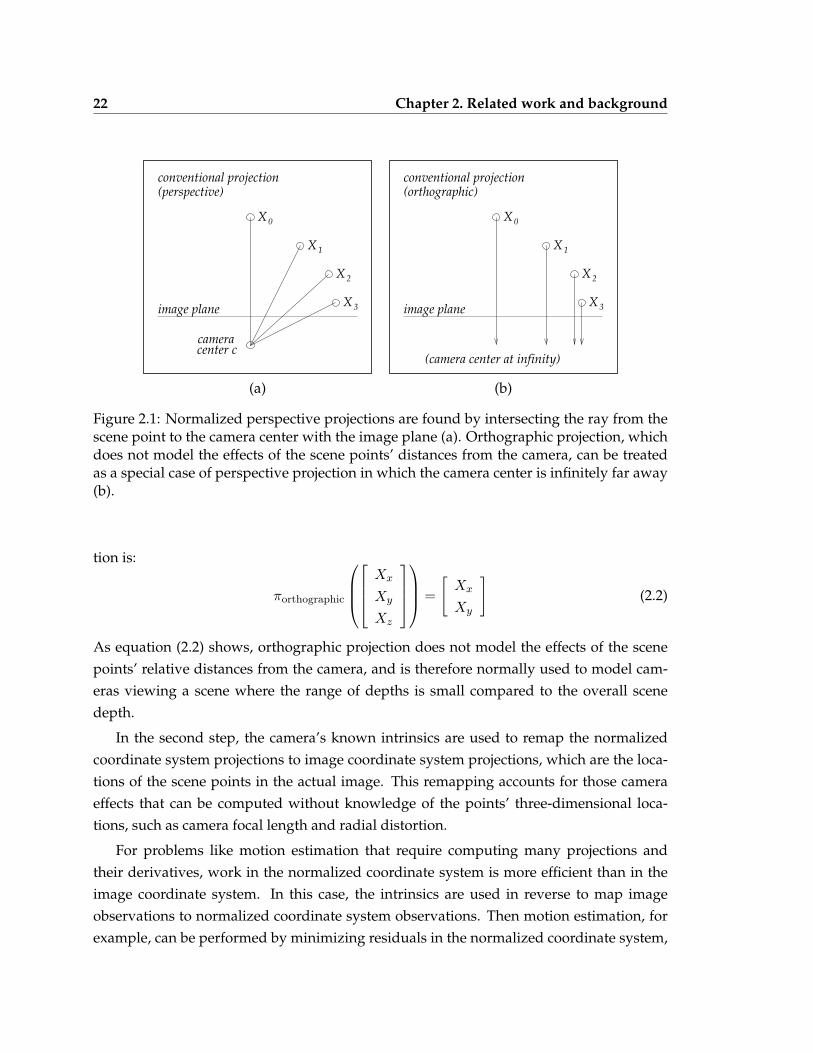
Figure 2.1: Normalized perspective projections are found by intersecting the ray from thescene point to the camera center with the image plane (a). Orthographic projection, whichdoes not model the effects of the scene points’ distances from the camera, can be treatedas a special case of perspective projection in which the camera center is infinitely far away(b).
tion is:
πorthographic
Xx
Xy
Xz
=
[Xx
Xy
](2.2)
As equation (2.2) shows, orthographic projection does not model the effects of the scenepoints’ relative distances from the camera, and is therefore normally used to model cam-eras viewing a scene where the range of depths is small compared to the overall scenedepth.
In the second step, the camera’s known intrinsics are used to remap the normalizedcoordinate system projections to image coordinate system projections, which are the loca-tions of the scene points in the actual image. This remapping accounts for those cameraeffects that can be computed without knowledge of the points’ three-dimensional loca-tions, such as camera focal length and radial distortion.
For problems like motion estimation that require computing many projections andtheir derivatives, work in the normalized coordinate system is more efficient than in theimage coordinate system. In this case, the intrinsics are used in reverse to map imageobservations to normalized coordinate system observations. Then motion estimation, forexample, can be performed by minimizing residuals in the normalized coordinate system,
2.10. Background: bundle adjustment 23
as discussed in Section 2.10 below.
Working in the normalized coordinate system also requires that covariances associ-ated with image system projections be normalized. If xi is an image projection, Ci thecovariance associated with xi, and xn the corresponding normalized projection, then acorresponding normalized covariance can found using:
Cn =∂xn
∂xiCi
(∂xn
∂xi
)T
(2.3)
Throughout this work, the intrinsics model described by Heikkila and Silven[27] hasbeen used to convert between normalized and image coordinate system projections, anda publicly available algorithm for estimating the parameters of this model from images ofa known target has been used to perform the camera calibration. Heikkila and Silven’smodel includes separate focal lengths for the x and y image directions, which togetheraccount for both focal length and rectangular pixels; skew between the x and y imageaxes; a three-term polynomial radial distortion model; and a tangential distortion model.Average calibration residuals between 0.2 pixels and 1 pixel are typical with this intrinsicsmodel and calibration algorithm.
The average residuals produced by Heikkila and Silven’s model are a significant im-provement over Tsai’s[58][59] older, but widely used, model and calibration. However,the residuals for individual calibration points using Heikkila and Silven’s model are often2 pixels or more, suggesting that this model does not completely model the camera overthe entire field of view. Because motion estimation from images can be sensitive to projec-tion errors of much less than 2 pixels, it would be worthwhile to investigate more accuratecamera intrinsics models in the future.
2.10 Background: bundle adjustment
Bundle adjustment[61][57] and nonlinear shape-from-motion[55] are similar methods forsimultaneously estimating camera motion and sparse scene structure from projections inan image sequence. These are batch algorithms, meaning that they use all the observationsfrom the image sequence at once, and can produce highly accurate estimates if the cameramodel and projection data are accurate.
This section briefly reviews a bundle adjustment algorithm suitable for use with anyconventional or omnidirectional projection model. This algorithm is used in several sub-sequent sections:
24 Chapter 2. Related work and background
• In Section 3.5, the algorithm is used with the omnidirectional projection model fromSection 3.3 to evaluate the omnidirectional camera calibration approach in Section3.4.
• The bundle adjustment error term forms one leg of the batch algorithm for estimatingmotion from image and inertial measurements described in Section 4.3.
• The algorithm is used on a prefix of the image sequence to initialize the recursive,image-only motion estimation algorithm described in Section 4.4.7.
• In Chapter 5, the algorithm is used to generate image-only motion estimates fromboth conventional and omnidirectional images for comparison with the image-and-inertial motion estimates.
• In Chapter 6, the algorithm is used to estimate epipolar geometry and detect mis-tracking within the tracker.
The algorithm uses Levenberg-Marquardt to minimize the error between observed pro-jections and predicted projections, with respect to the camera and point estimates. This sec-tion describes the error function; see [48] for the details of Levenberg-Marquardt, which iswidely used.
The error term is:χ2 =
∑i,j
Di,j(π(Wρi,ti(Xj)), xij) (2.4)
Equation (2.4) specifies an image reprojection error given the six degree of freedom camerapositions and three-dimensional point positions. In this error, the sum is over i and j,such that point j was observed in image i. xij is the observed projection of point j inimage i. ρi and ti are the rotation Euler angles and translation specifying the camera-to-world coordinate system transformation, respectively, at the time of image i; and Wρi,ti
is the corresponding world-to-camera transformation. Xj is the world coordinate systemlocation of point j, so that Wρi,ti(Xj) is location of point j in camera coordinate system i.
π gives the image projection of a three-dimensional point specified in the camera co-ordinate system. For conventional images, π might be the perspective projection or ortho-graphic projection. Section 3.3 below describes a projection model suitable for use withomnidirectional images.
The individual distance functions Di,j are Mahalanobis distances. If the operator π
produces image coordinate system projections (i.e., if π accounts for the camera focallength and other intrinsics), then reasonable choices for the associated covariances are di-rectional covariances determined using image texture in the vicinity of each feature[7][34],
2.10. Background: bundle adjustment 25
or isotropic covariances with σ = 1 pixels or σ = 2 pixels. However, π is normally chosento give projections in the normalized coordinate system. In this case, suitable covariancescan be found by converting the directional or isotropic image coordinate system covari-ances to normalized covariances as described in Section 2.9.
Levenberg-Marquardt is an iterative algorithm, and to ensure convergence, the initialestimate provided to the method must be sufficiently close to the solution. If a recursivemotion estimation algorithm is applicable, then a good recursive solution is a suitableinitial estimate for bundle adjustment. Each of the sections below that includes bundleadjustment results also describes how the initial estimates were computed.

Chapter 3
Motion from noncentralomnidirectional image sequences
3.1 Overview
Recent omnidirectional camera designs aim a conventional camera at a mirror that ex-pands the camera’s field of view, typically to 360◦ in azimuth and 90◦ to 140◦ in elevation.For camera motion estimation, there are two potential advantages to this wide field ofview. First, the wide view eliminates the sensitivity in motion estimates that may occurwith a conventional camera, such as the confusion between small rotational and smalltranslational motions. Second, tracked points are likely to be visible longer in an omnidi-rectional image sequence, which is helpful for motion estimation from long sequences.
To fully exploit these advantages, however, the omnidirectional camera’s projection(i.e., imaging) process must be accurately modeled. This chapter describes an approachfor modeling omnidirectional cameras, for calibrating omnidirectional cameras using thismodel, and for estimating camera motion from omnidirectional images using this model.Unlike existing methods, the projection model described in this chapter accommodatesboth single viewpoint omnidirectional cameras and the wider space of non-single-viewpoint,or noncentral cameras, described below. The method also accommodates known six degreeof freedom misalignment between the conventional camera and mirror that compose theomnidirectional camera.
This chapter is organized as follows. Single viewpoint and noncentral omnidirectionalcameras are briefly introduced in Section 3.2, and Section 3.3 describes the general om-nidirectional projection model. Sections 3.4 describes omnidirectional camera calibrationusing this model. Experimental results evaluating the model and calibration are given in
27
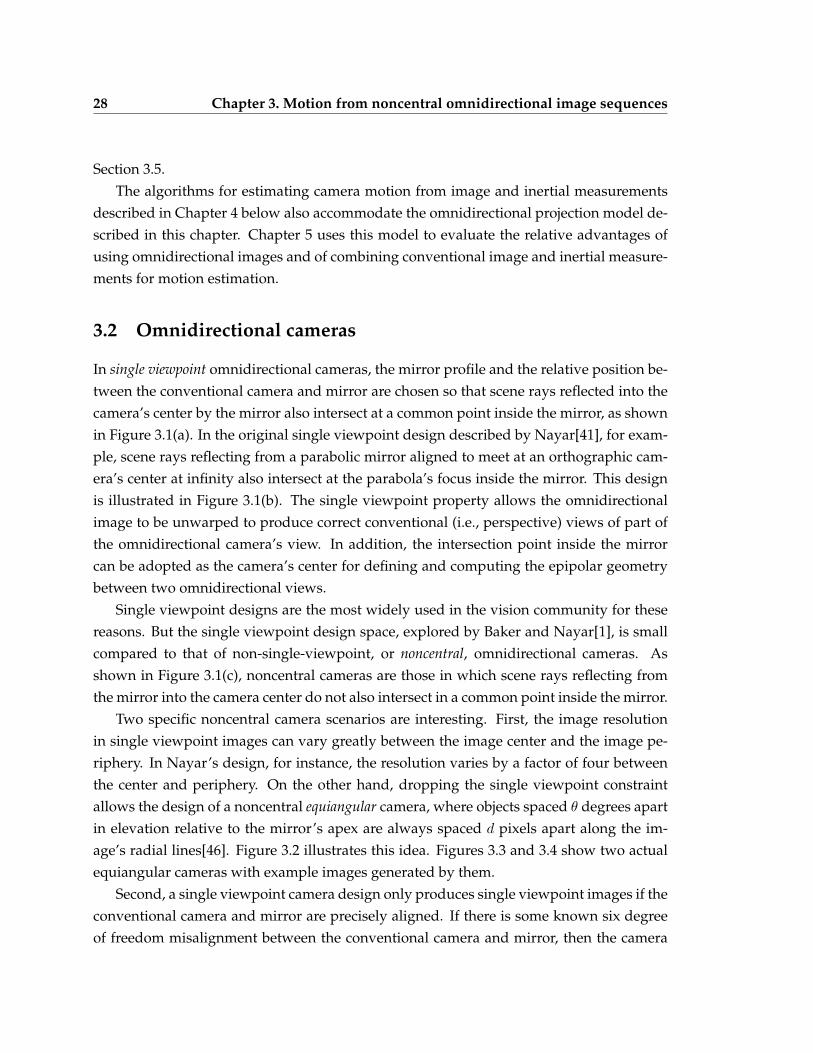
28 Chapter 3. Motion from noncentral omnidirectional image sequences
Section 3.5.The algorithms for estimating camera motion from image and inertial measurements
described in Chapter 4 below also accommodate the omnidirectional projection model de-scribed in this chapter. Chapter 5 uses this model to evaluate the relative advantages ofusing omnidirectional images and of combining conventional image and inertial measure-ments for motion estimation.
3.2 Omnidirectional cameras
In single viewpoint omnidirectional cameras, the mirror profile and the relative position be-tween the conventional camera and mirror are chosen so that scene rays reflected into thecamera’s center by the mirror also intersect at a common point inside the mirror, as shownin Figure 3.1(a). In the original single viewpoint design described by Nayar[41], for exam-ple, scene rays reflecting from a parabolic mirror aligned to meet at an orthographic cam-era’s center at infinity also intersect at the parabola’s focus inside the mirror. This designis illustrated in Figure 3.1(b). The single viewpoint property allows the omnidirectionalimage to be unwarped to produce correct conventional (i.e., perspective) views of part ofthe omnidirectional camera’s view. In addition, the intersection point inside the mirrorcan be adopted as the camera’s center for defining and computing the epipolar geometrybetween two omnidirectional views.
Single viewpoint designs are the most widely used in the vision community for thesereasons. But the single viewpoint design space, explored by Baker and Nayar[1], is smallcompared to that of non-single-viewpoint, or noncentral, omnidirectional cameras. Asshown in Figure 3.1(c), noncentral cameras are those in which scene rays reflecting fromthe mirror into the camera center do not also intersect in a common point inside the mirror.
Two specific noncentral camera scenarios are interesting. First, the image resolutionin single viewpoint images can vary greatly between the image center and the image pe-riphery. In Nayar’s design, for instance, the resolution varies by a factor of four betweenthe center and periphery. On the other hand, dropping the single viewpoint constraintallows the design of a noncentral equiangular camera, where objects spaced θ degrees apartin elevation relative to the mirror’s apex are always spaced d pixels apart along the im-age’s radial lines[46]. Figure 3.2 illustrates this idea. Figures 3.3 and 3.4 show two actualequiangular cameras with example images generated by them.
Second, a single viewpoint camera design only produces single viewpoint images if theconventional camera and mirror are precisely aligned. If there is some known six degreeof freedom misalignment between the conventional camera and mirror, then the camera
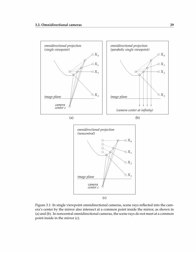
3.2. Omnidirectional cameras 29
cameracenter c
X
X
X
image plane
X
0
1
2
3
omnidirectional projection(single viewpoint)
X
X
X
image plane
(camera center at infinity)
omnidirectional projection(parabolic single viewpoint)
0
X 1
2
3
(a) (b)
cameracenter c
Ximage plane
omnidirectional projection(noncentral)
X
X
X 0
1
2
3
(c)
Figure 3.1: In single viewpoint omnidirectional cameras, scene rays reflected into the cam-era’s center by the mirror also intersect at a common point inside the mirror, as shown in(a) and (b). In noncentral omnidirectional cameras, the scene rays do not meet at a commonpoint inside in the mirror (c).
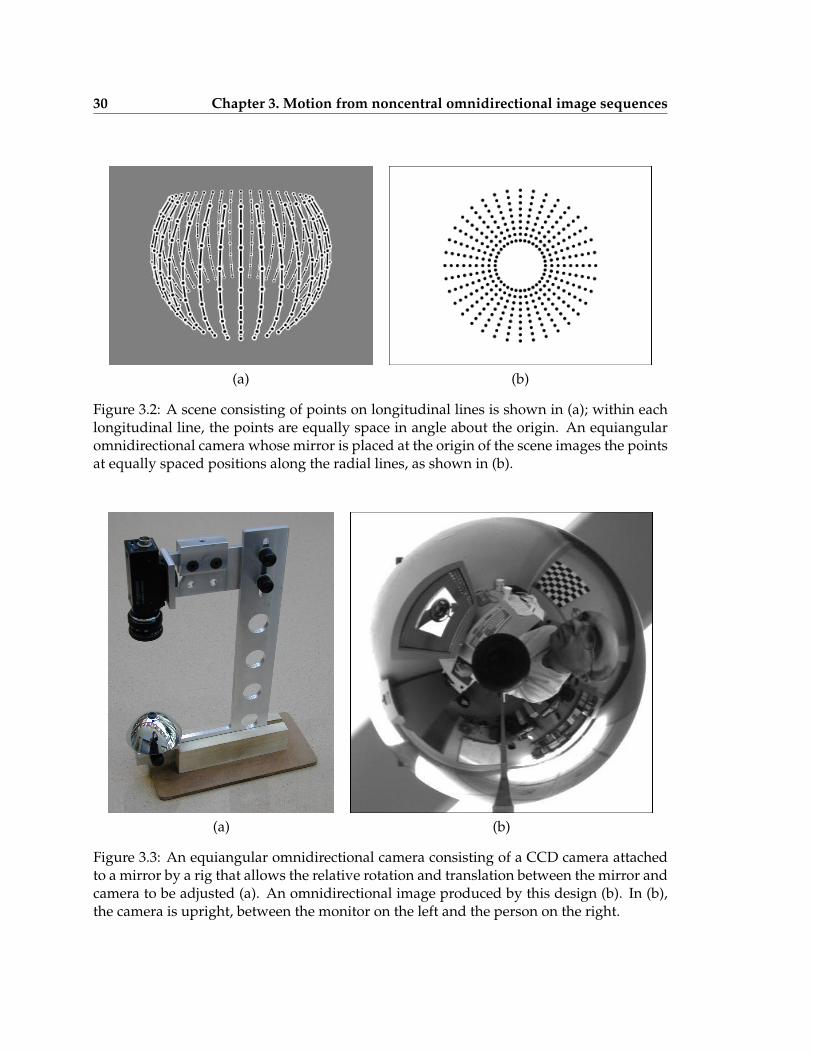
30 Chapter 3. Motion from noncentral omnidirectional image sequences
(a) (b)
Figure 3.2: A scene consisting of points on longitudinal lines is shown in (a); within eachlongitudinal line, the points are equally space in angle about the origin. An equiangularomnidirectional camera whose mirror is placed at the origin of the scene images the pointsat equally spaced positions along the radial lines, as shown in (b).
(a) (b)
Figure 3.3: An equiangular omnidirectional camera consisting of a CCD camera attachedto a mirror by a rig that allows the relative rotation and translation between the mirror andcamera to be adjusted (a). An omnidirectional image produced by this design (b). In (b),the camera is upright, between the monitor on the left and the person on the right.
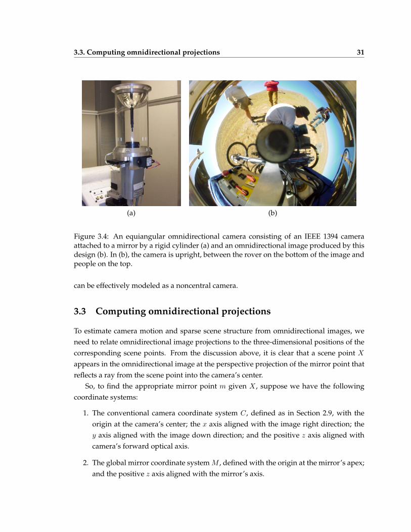
3.3. Computing omnidirectional projections 31
(a) (b)
Figure 3.4: An equiangular omnidirectional camera consisting of an IEEE 1394 cameraattached to a mirror by a rigid cylinder (a) and an omnidirectional image produced by thisdesign (b). In (b), the camera is upright, between the rover on the bottom of the image andpeople on the top.
can be effectively modeled as a noncentral camera.
3.3 Computing omnidirectional projections
To estimate camera motion and sparse scene structure from omnidirectional images, weneed to relate omnidirectional image projections to the three-dimensional positions of thecorresponding scene points. From the discussion above, it is clear that a scene point X
appears in the omnidirectional image at the perspective projection of the mirror point thatreflects a ray from the scene point into the camera’s center.
So, to find the appropriate mirror point m given X , suppose we have the followingcoordinate systems:
1. The conventional camera coordinate system C, defined as in Section 2.9, with theorigin at the camera’s center; the x axis aligned with the image right direction; they axis aligned with the image down direction; and the positive z axis aligned withcamera’s forward optical axis.
2. The global mirror coordinate system M , defined with the origin at the mirror’s apex;and the positive z axis aligned with the mirror’s axis.
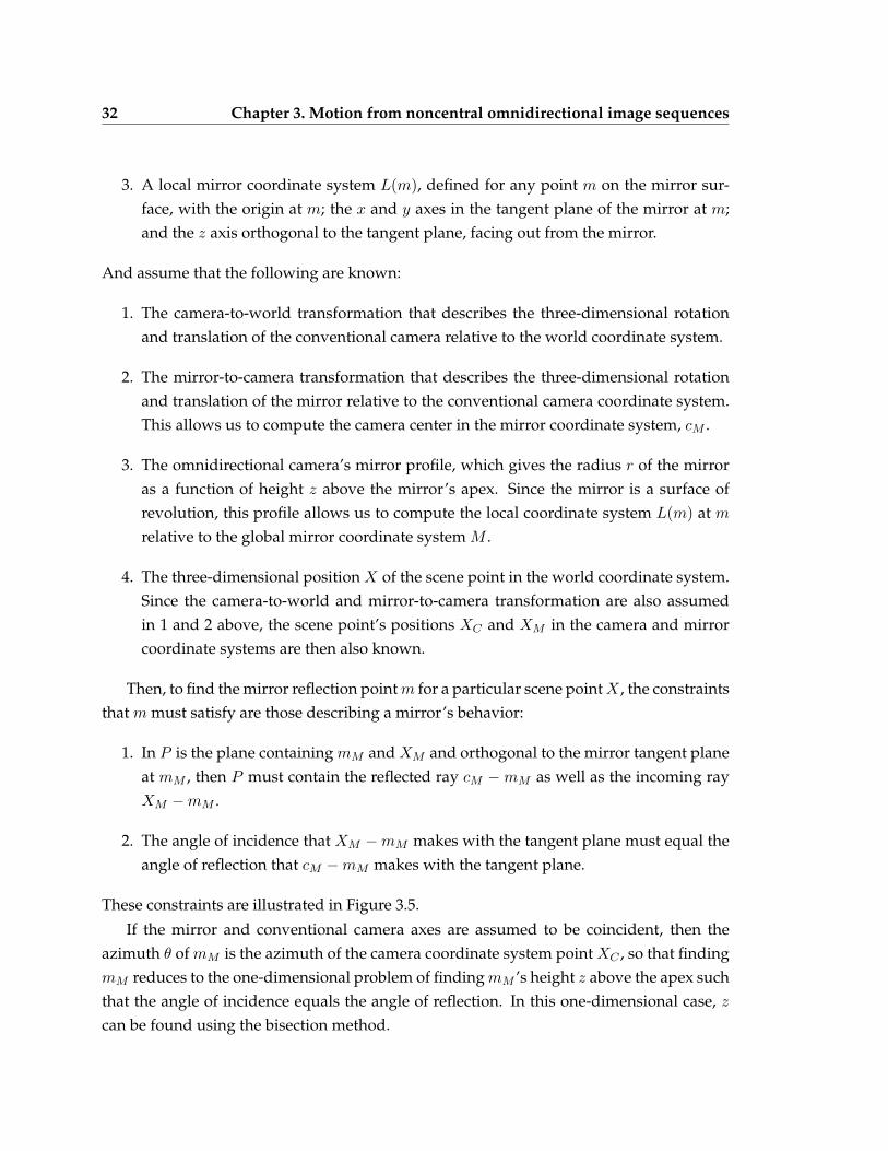
32 Chapter 3. Motion from noncentral omnidirectional image sequences
3. A local mirror coordinate system L(m), defined for any point m on the mirror sur-face, with the origin at m; the x and y axes in the tangent plane of the mirror at m;and the z axis orthogonal to the tangent plane, facing out from the mirror.
And assume that the following are known:
1. The camera-to-world transformation that describes the three-dimensional rotationand translation of the conventional camera relative to the world coordinate system.
2. The mirror-to-camera transformation that describes the three-dimensional rotationand translation of the mirror relative to the conventional camera coordinate system.This allows us to compute the camera center in the mirror coordinate system, cM .
3. The omnidirectional camera’s mirror profile, which gives the radius r of the mirroras a function of height z above the mirror’s apex. Since the mirror is a surface ofrevolution, this profile allows us to compute the local coordinate system L(m) at m
relative to the global mirror coordinate system M .
4. The three-dimensional position X of the scene point in the world coordinate system.Since the camera-to-world and mirror-to-camera transformation are also assumedin 1 and 2 above, the scene point’s positions XC and XM in the camera and mirrorcoordinate systems are then also known.
Then, to find the mirror reflection point m for a particular scene point X , the constraintsthat m must satisfy are those describing a mirror’s behavior:
1. In P is the plane containing mM and XM and orthogonal to the mirror tangent planeat mM , then P must contain the reflected ray cM −mM as well as the incoming rayXM −mM .
2. The angle of incidence that XM −mM makes with the tangent plane must equal theangle of reflection that cM −mM makes with the tangent plane.
These constraints are illustrated in Figure 3.5.
If the mirror and conventional camera axes are assumed to be coincident, then theazimuth θ of mM is the azimuth of the camera coordinate system point XC , so that findingmM reduces to the one-dimensional problem of finding mM ’s height z above the apex suchthat the angle of incidence equals the angle of reflection. In this one-dimensional case, z
can be found using the bisection method.
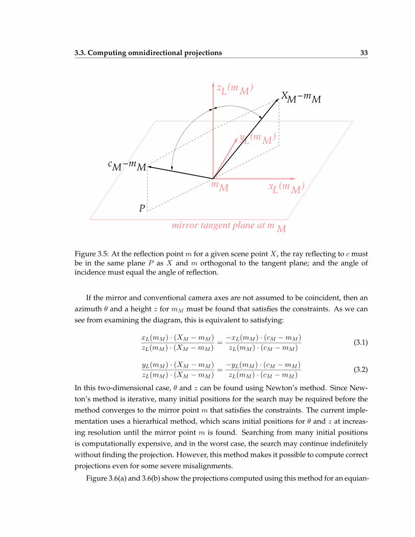
3.3. Computing omnidirectional projections 33
L(m M)y
mM
mM
xL(m
P
−MX
Mc −
mM
zL(m M
M)
)
mirror tangent plane at m M
Figure 3.5: At the reflection point m for a given scene point X , the ray reflecting to c mustbe in the same plane P as X and m orthogonal to the tangent plane; and the angle ofincidence must equal the angle of reflection.
If the mirror and conventional camera axes are not assumed to be coincident, then anazimuth θ and a height z for mM must be found that satisfies the constraints. As we cansee from examining the diagram, this is equivalent to satisfying:
xL(mM ) · (XM −mM )zL(mM ) · (XM −mM )
=−xL(mM ) · (cM −mM )zL(mM ) · (cM −mM )
(3.1)
yL(mM ) · (XM −mM )zL(mM ) · (XM −mM )
=−yL(mM ) · (cM −mM )zL(mM ) · (cM −mM )
(3.2)
In this two-dimensional case, θ and z can be found using Newton’s method. Since New-ton’s method is iterative, many initial positions for the search may be required before themethod converges to the mirror point m that satisfies the constraints. The current imple-mentation uses a hierarhical method, which scans initial positions for θ and z at increas-ing resolution until the mirror point m is found. Searching from many initial positionsis computationally expensive, and in the worst case, the search may continue indefinitelywithout finding the projection. However, this method makes it possible to compute correctprojections even for some severe misalignments.
Figure 3.6(a) and 3.6(b) show the projections computed using this method for an equian-
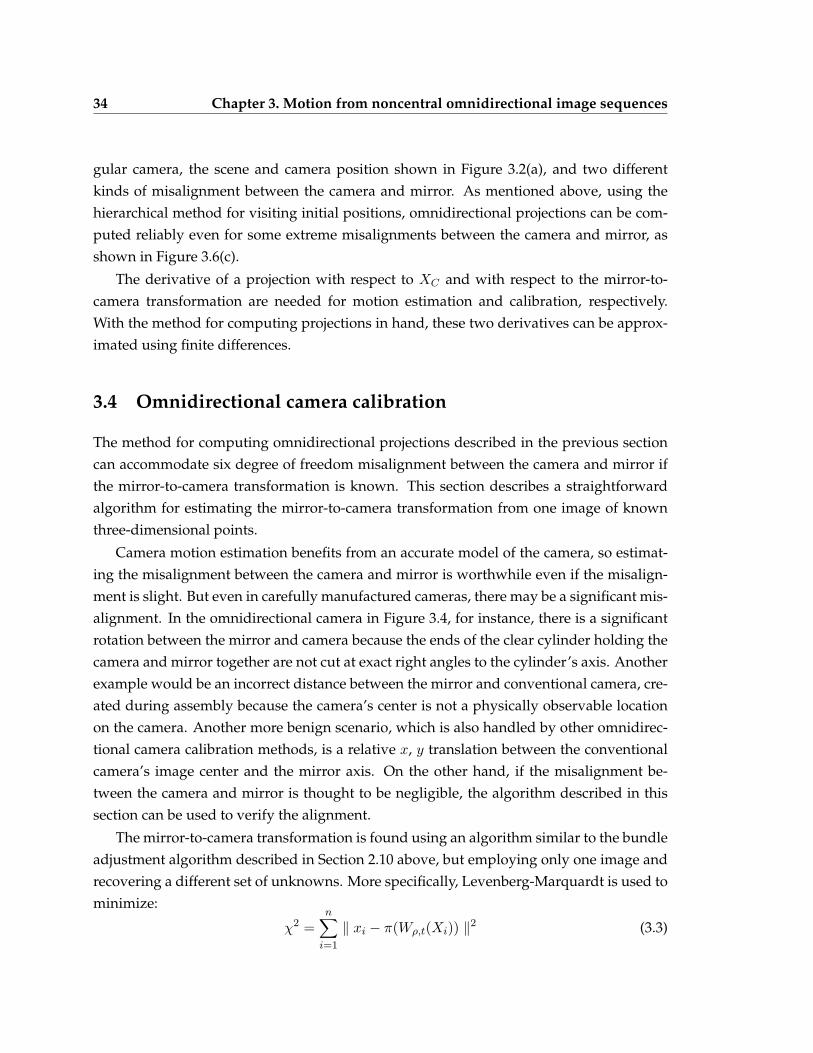
34 Chapter 3. Motion from noncentral omnidirectional image sequences
gular camera, the scene and camera position shown in Figure 3.2(a), and two differentkinds of misalignment between the camera and mirror. As mentioned above, using thehierarchical method for visiting initial positions, omnidirectional projections can be com-puted reliably even for some extreme misalignments between the camera and mirror, asshown in Figure 3.6(c).
The derivative of a projection with respect to XC and with respect to the mirror-to-camera transformation are needed for motion estimation and calibration, respectively.With the method for computing projections in hand, these two derivatives can be approx-imated using finite differences.
3.4 Omnidirectional camera calibration
The method for computing omnidirectional projections described in the previous sectioncan accommodate six degree of freedom misalignment between the camera and mirror ifthe mirror-to-camera transformation is known. This section describes a straightforwardalgorithm for estimating the mirror-to-camera transformation from one image of knownthree-dimensional points.
Camera motion estimation benefits from an accurate model of the camera, so estimat-ing the misalignment between the camera and mirror is worthwhile even if the misalign-ment is slight. But even in carefully manufactured cameras, there may be a significant mis-alignment. In the omnidirectional camera in Figure 3.4, for instance, there is a significantrotation between the mirror and camera because the ends of the clear cylinder holding thecamera and mirror together are not cut at exact right angles to the cylinder’s axis. Anotherexample would be an incorrect distance between the mirror and conventional camera, cre-ated during assembly because the camera’s center is not a physically observable locationon the camera. Another more benign scenario, which is also handled by other omnidirec-tional camera calibration methods, is a relative x, y translation between the conventionalcamera’s image center and the mirror axis. On the other hand, if the misalignment be-tween the camera and mirror is thought to be negligible, the algorithm described in thissection can be used to verify the alignment.
The mirror-to-camera transformation is found using an algorithm similar to the bundleadjustment algorithm described in Section 2.10 above, but employing only one image andrecovering a different set of unknowns. More specifically, Levenberg-Marquardt is used tominimize:
χ2 =n∑
i=1
‖ xi − π(Wρ,t(Xi)) ‖2 (3.3)
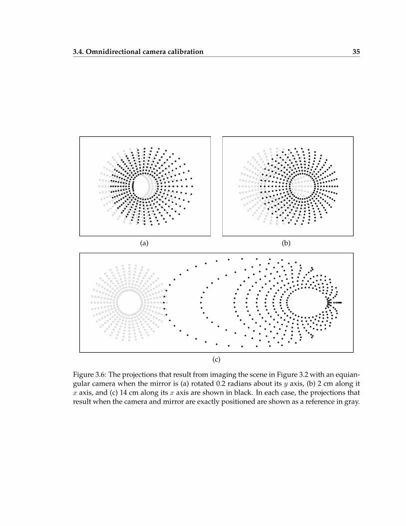
3.4. Omnidirectional camera calibration 35
(a) (b)
(c)
Figure 3.6: The projections that result from imaging the scene in Figure 3.2 with an equian-gular camera when the mirror is (a) rotated 0.2 radians about its y axis, (b) 2 cm along itx axis, and (c) 14 cm along its x axis are shown in black. In each case, the projections thatresult when the camera and mirror are exactly positioned are shown as a reference in gray.
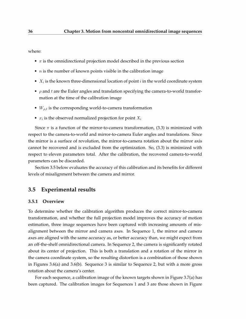
36 Chapter 3. Motion from noncentral omnidirectional image sequences
where:
• π is the omnidirectional projection model described in the previous section
• n is the number of known points visible in the calibration image
• Xi is the known three-dimensional location of point i in the world coordinate system
• ρ and t are the Euler angles and translation specifying the camera-to-world transfor-mation at the time of the calibration image
• Wρ,t is the corresponding world-to-camera transformation
• xi is the observed normalized projection for point Xi
Since π is a function of the mirror-to-camera transformation, (3.3) is minimized withrespect to the camera-to-world and mirror-to-camera Euler angles and translations. Sincethe mirror is a surface of revolution, the mirror-to-camera rotation about the mirror axiscannot be recovered and is excluded from the optimization. So, (3.3) is minimized withrespect to eleven parameters total. After the calibration, the recovered camera-to-worldparameters can be discarded.
Section 3.5 below evaluates the accuracy of this calibration and its benefits for differentlevels of misalignment between the camera and mirror.
3.5 Experimental results
3.5.1 Overview
To determine whether the calibration algorithm produces the correct mirror-to-cameratransformation, and whether the full projection model improves the accuracy of motionestimation, three image sequences have been captured with increasing amounts of mis-alignment between the mirror and camera axes. In Sequence 1, the mirror and cameraaxes are aligned with the same accuracy as, or better accuracy than, we might expect froman off-the-shelf omnidirectional camera. In Sequence 2, the camera is significantly rotatedabout its center of projection. This is both a translation and a rotation of the mirror inthe camera coordinate system, so the resulting distortion is a combination of those shownin Figures 3.6(a) and 3.6(b). Sequence 3 is similar to Sequence 2, but with a more grossrotation about the camera’s center.
For each sequence, a calibration image of the known targets shown in Figure 3.7(a) hasbeen captured. The calibration images for Sequences 1 and 3 are those shown in Figure
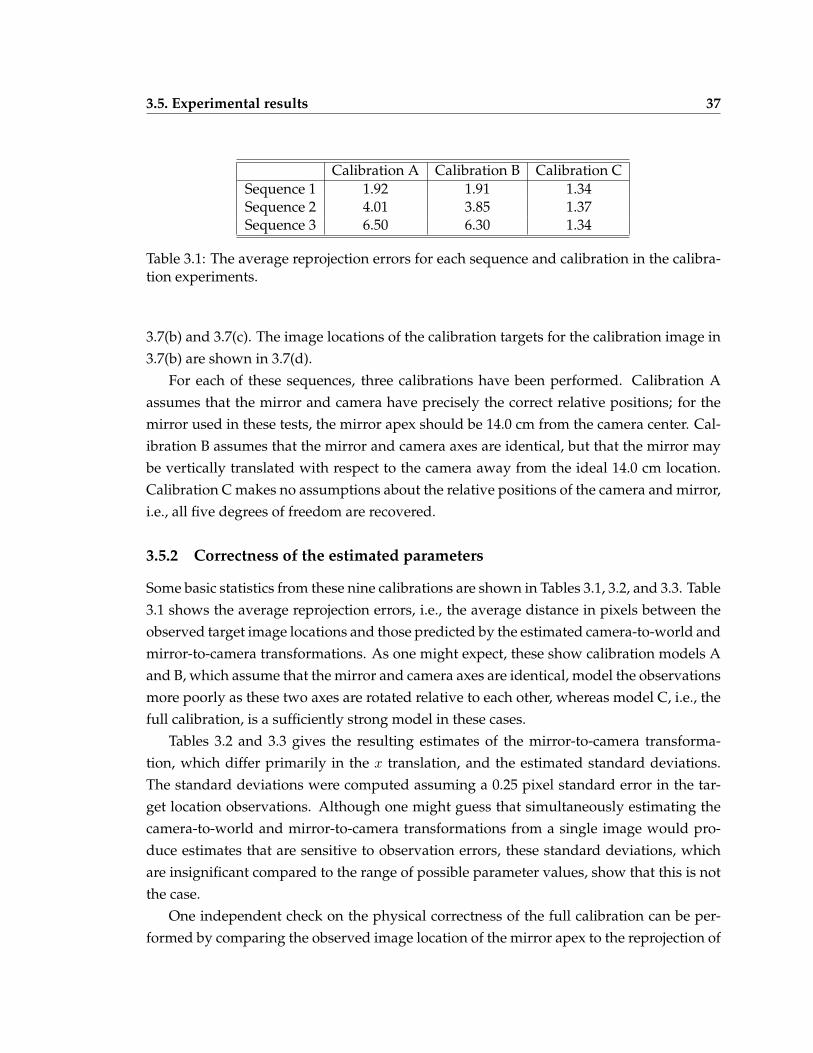
3.5. Experimental results 37
Calibration A Calibration B Calibration CSequence 1 1.92 1.91 1.34Sequence 2 4.01 3.85 1.37Sequence 3 6.50 6.30 1.34
Table 3.1: The average reprojection errors for each sequence and calibration in the calibra-tion experiments.
3.7(b) and 3.7(c). The image locations of the calibration targets for the calibration image in3.7(b) are shown in 3.7(d).
For each of these sequences, three calibrations have been performed. Calibration Aassumes that the mirror and camera have precisely the correct relative positions; for themirror used in these tests, the mirror apex should be 14.0 cm from the camera center. Cal-ibration B assumes that the mirror and camera axes are identical, but that the mirror maybe vertically translated with respect to the camera away from the ideal 14.0 cm location.Calibration C makes no assumptions about the relative positions of the camera and mirror,i.e., all five degrees of freedom are recovered.
3.5.2 Correctness of the estimated parameters
Some basic statistics from these nine calibrations are shown in Tables 3.1, 3.2, and 3.3. Table3.1 shows the average reprojection errors, i.e., the average distance in pixels between theobserved target image locations and those predicted by the estimated camera-to-world andmirror-to-camera transformations. As one might expect, these show calibration models Aand B, which assume that the mirror and camera axes are identical, model the observationsmore poorly as these two axes are rotated relative to each other, whereas model C, i.e., thefull calibration, is a sufficiently strong model in these cases.
Tables 3.2 and 3.3 gives the resulting estimates of the mirror-to-camera transforma-tion, which differ primarily in the x translation, and the estimated standard deviations.The standard deviations were computed assuming a 0.25 pixel standard error in the tar-get location observations. Although one might guess that simultaneously estimating thecamera-to-world and mirror-to-camera transformations from a single image would pro-duce estimates that are sensitive to observation errors, these standard deviations, whichare insignificant compared to the range of possible parameter values, show that this is notthe case.
One independent check on the physical correctness of the full calibration can be per-formed by comparing the observed image location of the mirror apex to the reprojection of
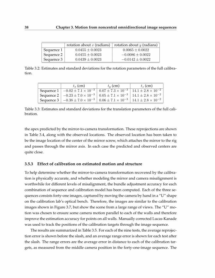
38 Chapter 3. Motion from noncentral omnidirectional image sequences
rotation about x (radians) rotation about y (radians)Sequence 1 0.0455± 0.0023 0.0065± 0.0022Sequence 2 0.0455± 0.0023 −0.0086± 0.0022Sequence 3 0.0439± 0.0023 −0.0142± 0.0022
Table 3.2: Estimates and standard deviations for the rotation parameters of the full calibra-tion.
tx (cm) ty (cm) tz (cm)Sequence 1 −0.02± 7.1× 10⁻³ 0.07± 7.3× 10⁻³ 14.1± 2.8× 10⁻²
Sequence 2 −0.23± 7.0× 10⁻³ 0.05± 7.1× 10⁻³ 14.1± 2.8× 10⁻²
Sequence 3 −0.38± 7.0× 10⁻³ 0.06± 7.1× 10⁻³ 14.1± 2.8× 10⁻²
Table 3.3: Estimates and standard deviations for the translation parameters of the full cali-bration.
the apex predicted by the mirror-to-camera transformation. These reprojections are shownin Table 3.4, along with the observed locations. The observed location has been taken tobe the image location of the center of the mirror screw, which attaches the mirror to the rigand passes through the mirror axis. In each case the predicted and observed centers arequite close.
3.5.3 Effect of calibration on estimated motion and structure
To help determine whether the mirror-to-camera transformation recovered by the calibra-tion is physically accurate, and whether modeling the mirror and camera misalignment isworthwhile for different levels of misalignment, the bundle adjustment accuracy for eachcombination of sequence and calibration model has been computed. Each of the three se-quences consists forty-one images, captured by moving the camera by hand in a “U” shapeon the calibration lab’s optical bench. Therefore, the images are similar to the calibrationimages shown in Figure 3.7, but show the scene from a large range of views. The “U” mo-tion was chosen to ensure some camera motion parallel to each of the walls and thereforeimprove the estimation accuracy for points on all walls. Manually corrected Lucas-Kanadewas used to track the positions of the calibration targets through the image sequence.
The results are summarized in Table 3.5. For each of the nine tests, the average reprojec-tion error is shown before the slash, and an average range error is shown for each test afterthe slash. The range errors are the average error in distance to each of the calibration tar-gets, as measured from the middle camera position in the forty-one-image sequence. The
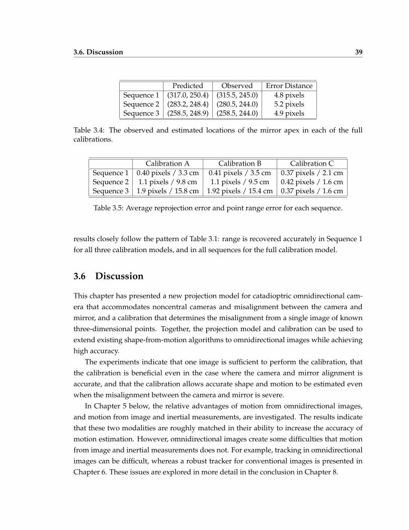
3.6. Discussion 39
Predicted Observed Error DistanceSequence 1 (317.0, 250.4) (315.5, 245.0) 4.8 pixelsSequence 2 (283.2, 248.4) (280.5, 244.0) 5.2 pixelsSequence 3 (258.5, 248.9) (258.5, 244.0) 4.9 pixels
Table 3.4: The observed and estimated locations of the mirror apex in each of the fullcalibrations.
Calibration A Calibration B Calibration CSequence 1 0.40 pixels / 3.3 cm 0.41 pixels / 3.5 cm 0.37 pixels / 2.1 cmSequence 2 1.1 pixels / 9.8 cm 1.1 pixels / 9.5 cm 0.42 pixels / 1.6 cmSequence 3 1.9 pixels / 15.8 cm 1.92 pixels / 15.4 cm 0.37 pixels / 1.6 cm
Table 3.5: Average reprojection error and point range error for each sequence.
results closely follow the pattern of Table 3.1: range is recovered accurately in Sequence 1for all three calibration models, and in all sequences for the full calibration model.
3.6 Discussion
This chapter has presented a new projection model for catadioptric omnidirectional cam-era that accommodates noncentral cameras and misalignment between the camera andmirror, and a calibration that determines the misalignment from a single image of knownthree-dimensional points. Together, the projection model and calibration can be used toextend existing shape-from-motion algorithms to omnidirectional images while achievinghigh accuracy.
The experiments indicate that one image is sufficient to perform the calibration, thatthe calibration is beneficial even in the case where the camera and mirror alignment isaccurate, and that the calibration allows accurate shape and motion to be estimated evenwhen the misalignment between the camera and mirror is severe.
In Chapter 5 below, the relative advantages of motion from omnidirectional images,and motion from image and inertial measurements, are investigated. The results indicatethat these two modalities are roughly matched in their ability to increase the accuracy ofmotion estimation. However, omnidirectional images create some difficulties that motionfrom image and inertial measurements does not. For example, tracking in omnidirectionalimages can be difficult, whereas a robust tracker for conventional images is presented inChapter 6. These issues are explored in more detail in the conclusion in Chapter 8.
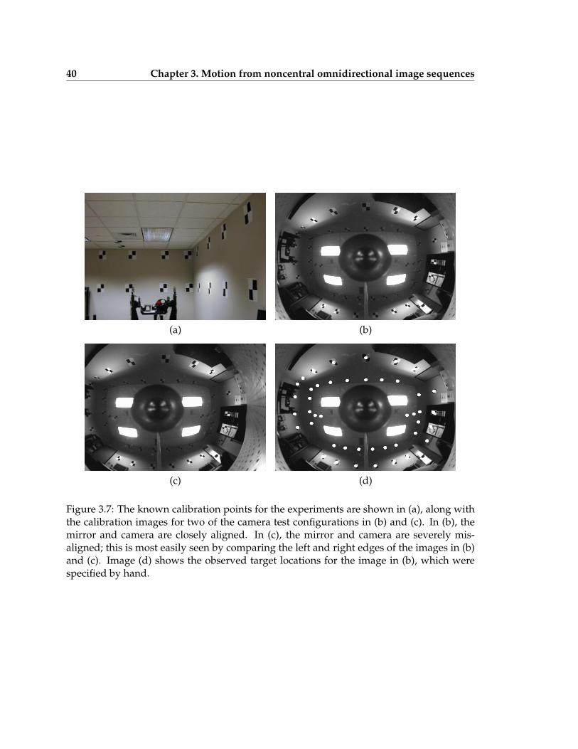
40 Chapter 3. Motion from noncentral omnidirectional image sequences
(a) (b)
(c) (d)
Figure 3.7: The known calibration points for the experiments are shown in (a), along withthe calibration images for two of the camera test configurations in (b) and (c). In (b), themirror and camera are closely aligned. In (c), the mirror and camera are severely mis-aligned; this is most easily seen by comparing the left and right edges of the images in (b)and (c). Image (d) shows the observed target locations for the image in (b), which werespecified by hand.
Chapter 4
Motion from image and inertialmeasurements: algorithms
4.1 Overview
Cameras and inertial sensors are each good candidates for autonomous vehicle navigation,modeling from video, and other applications that require six degree of freedom motionestimation. In addition, cameras and inertial sensors are good candidates to be deployedtogether, since in addition to the obvious advantage of redundant measurements, eachcan be used to resolve the ambiguities in the estimated motion that result from using theother modality alone. For instance, image measurements can counteract the error thataccumulates when integrating inertial readings, whereas inertial sensors can eliminate theerrors in motion that result from estimating motion from too few image measurements.
This chapter considers the specific problem of estimating sensor motion and other un-knowns from image, gyro, and accelerometer measurements, in environments withoutknown fiducials and without external positioning systems such as GPS. Accurate mo-tion estimation under these circumstances has a number of potential applications in au-tonomous navigation underwater, indoors, in rubble, in the urban canyon, or on Mars,which all preclude the use of global positioning; and in modeling from video. Some im-portant potential applications preclude the use of precise inertial navigation systems, suchas micro air vehicle navigation, where weight and cost are limiting factors. So, this workspecifically focuses on the use of lightweight and inexpensive inertial sensors.
This chapter presents two algorithms for estimating sensor motion and scene struc-ture from image and inertial measurements. The first is a batch algorithm that generatesestimates of the sensor motion, scene structure, and other parameters by considering all
41
42 Chapter 4. Motion from image and inertial measurements: algorithms
of the image and inertial measurements simultaneously. In many applications, this batchestimate is of interest in its own right. In others, the batch estimate is important in un-derstanding the best quality we can expect given a particular sensor configuration, vehiclemotion, environment, and set of observations, and in measuring the inherent sensitivity ofthe estimate with respect to random observation errors.
Because the batch method uses all of the measurements from an observation sequencesimultaneously, it requires that all of the observations be available before computationbegins. The second algorithm is a recursive method that estimates sensor motion, scenestructure, and other parameters from image, gyro, and accelerometer measurements asthey become available, and is therefore suitable for long or “infinite” image sequences.This algorithm is a multirate method, meaning that image measurements and inertialmeasurements are processed by separate update steps, which allows the higher rate ofinertial measurements to be exploited. Unlike many methods for motion estimation thatuse tracked image point features as measurements, the recursive method also includes amechanism for incorporating points that become visible after initialization while main-taining an accurate state covariance estimate. This capability is essential for operation onmost real image sequences.
This chapter is organized as follows. Section 4.2 reviews the complementary natureof image and inertial measurements in more detail. Sections 4.3 and 4.4 detail the batchand recursive algorithms, respectively. An experimental evaluation of these algorithms isgiven in Chapter 5 below.
4.2 Motion from image or inertial measurements alone
Six degree of freedom motion estimates can be generated from either image or inertialmeasurements. Integrating gyros and accelerometer outputs once and twice, respectively,produces estimates of the sensors’ rotation and translation. Similarly, camera motion andsparse scene structure can be simultaneously estimated from image measurements usinga method such as the bundle adjustment algorithm described in Section 2.10 above.
However, both approaches are error prone. Both unmodeled nonlinearity and noisein inertial sensor outputs cause these estimates to drift with time. In addition, gyro andaccelerometer outputs depend on biases that change with time, and accelerometer outputsdepend on the orientation of the sensor relative to gravity as well as the acceleration. So,these sensors cannot produce accurate motion estimates without some means of correctionand of estimating these additional unknowns.
On the other hand, simultaneous estimation of camera motion and sparse scene struc-
4.3. Batch algorithm 43
ture from images is brittle in practice. For many motions or environments, the estimatesfrom these algorithms can be sensitive to random observation errors and errors in cali-bration. In image sequences where features enter and leave the sequence at a high rate,estimates from shape-from-motion can be sensitive to the number of tracked features andthe rate of feature reextraction. Furthermore, motion estimates in this scenario will drift,just as estimates from inertial sensors will drift, because no one feature serves as a globalreference of the position. In addition, image observations alone provide no mechanism fordetermining the global scale of the estimate.
In both cases, the estimated motion can have gross errors. So naive methods for com-bining image and inertial measurements, such as averaging the estimates produced byeach modality individually, are only likely to produce a third poor estimate. Instead, algo-rithms for estimating motion from image and inertial measurements should only generateestimates that are consistent with both sets of observations simultaneously. The algorithmsin this chapter take this approach.
4.3 Batch algorithm
4.3.1 Overview
The batch algorithm for motion estimation from image and inertial measurements findsestimates of the sensor motion and other unknowns using the entire observation sequencefrom a camera, rate gyro, and accelerometer simultaneously. As shown in Figure 4.1(a),the algorithm estimates the sensor rig rotation, translation, and linear velocity at the timeof each image; the three-dimensional position of each point observed in the image se-quence; the gravity vector with respect to the world coordinate system; and the gyro andaccelerometer biases.
More specifically, the algorithm uses Levenberg-Marquardt to minimize a combinedimage and inertial error function. Since Levenberg-Marquardt is widely used, this sectionconcentrates on the error function; see [48] for a discussion of Levenberg-Marquardt. Theerror function is:
Ecombined = Eimage + Einertial + Eprior (4.1)
The image error Eimage is the χ2 bundle adjustment error described in Section 2.10. TheEinertial and Eprior terms of this error are described in the following subsections.
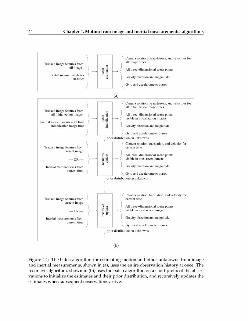
44 Chapter 4. Motion from image and inertial measurements: algorithms
bat
ch
Tracked image features from
Inertial measurements forall times
all images
Gyro and accelerometer biases
Gravity direction and magnitude
All three−dimensional scene points
Camera rotations, translations, and velocities forall image times
esti
mat
ion
(a)
bat
chin
itia
liza
tio
n
Inertial measurements until finalinitialization image time
Tracked image features fromall initialization images All three−dimensional scene points
Camera rotations, translations, and velocities forall initialization image times
Gravity direction and magnitude
Gyro and accelerometer biases
prior distribution on unknowns
All three−dimensional scene points
Camera rotation, translation, and velocity for
Gravity direction and magnitude
Gyro and accelerometer biases
up
dat
ere
curs
ive
−− OR −−
Tracked image features fromcurrent image
Inertial measurements fromcurrent time
current time
visible in most recent image
prior distribution on unknowns
visible in initialization images
(b)
Figure 4.1: The batch algorithm for estimating motion and other unknowns from imageand inertial measurements, shown in (a), uses the entire observation history at once. Therecursive algorithm, shown in (b), uses the batch algorithm on a short prefix of the obser-vations to initialize the estimates and their prior distribution, and recursively updates theestimates when subsequent observations arrive.
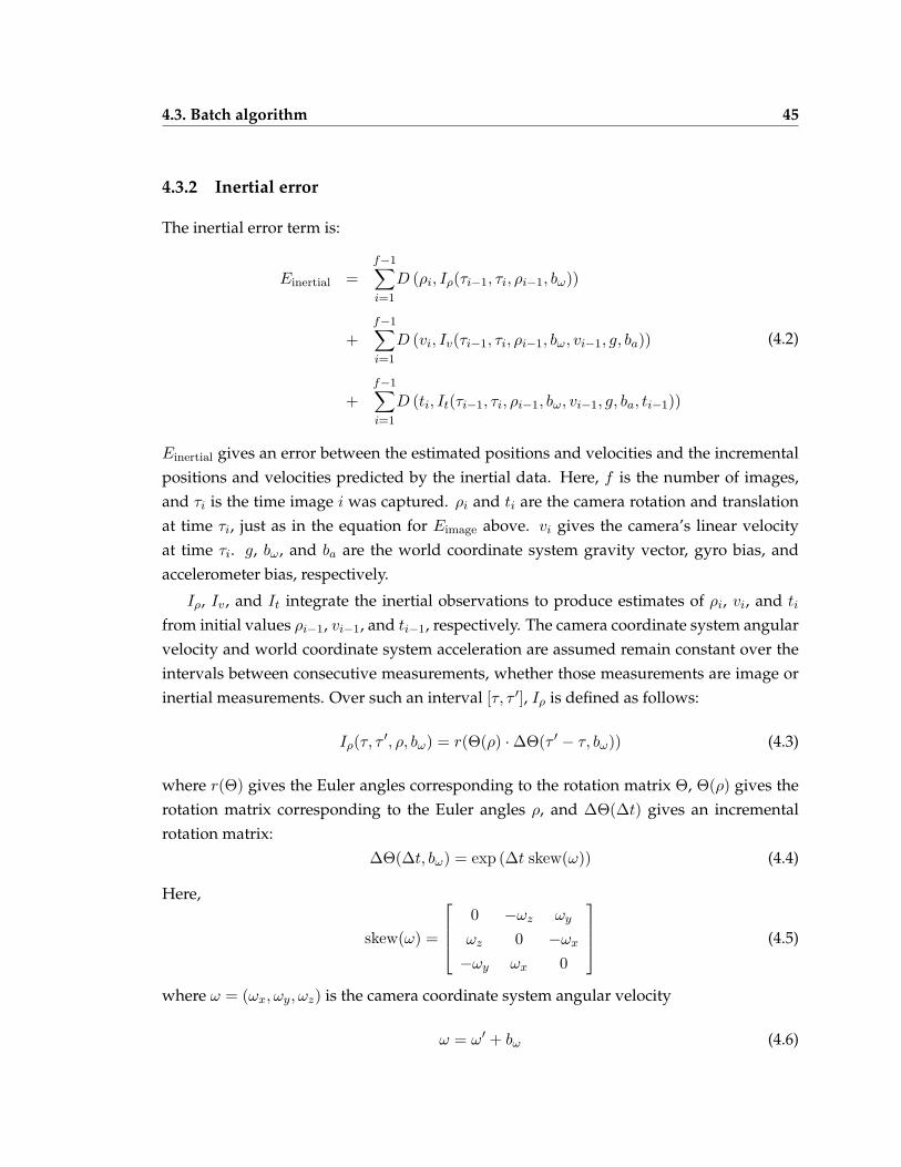
4.3. Batch algorithm 45
4.3.2 Inertial error
The inertial error term is:
Einertial =f−1∑i=1
D (ρi, Iρ(τi−1, τi, ρi−1, bω))
+f−1∑i=1
D (vi, Iv(τi−1, τi, ρi−1, bω, vi−1, g, ba))
+f−1∑i=1
D (ti, It(τi−1, τi, ρi−1, bω, vi−1, g, ba, ti−1))
(4.2)
Einertial gives an error between the estimated positions and velocities and the incrementalpositions and velocities predicted by the inertial data. Here, f is the number of images,and τi is the time image i was captured. ρi and ti are the camera rotation and translationat time τi, just as in the equation for Eimage above. vi gives the camera’s linear velocityat time τi. g, bω, and ba are the world coordinate system gravity vector, gyro bias, andaccelerometer bias, respectively.
Iρ, Iv, and It integrate the inertial observations to produce estimates of ρi, vi, and ti
from initial values ρi−1, vi−1, and ti−1, respectively. The camera coordinate system angularvelocity and world coordinate system acceleration are assumed remain constant over theintervals between consecutive measurements, whether those measurements are image orinertial measurements. Over such an interval [τ, τ ′], Iρ is defined as follows:
Iρ(τ, τ ′, ρ, bω) = r(Θ(ρ) ·∆Θ(τ ′ − τ, bω)) (4.3)
where r(Θ) gives the Euler angles corresponding to the rotation matrix Θ, Θ(ρ) gives therotation matrix corresponding to the Euler angles ρ, and ∆Θ(∆t) gives an incrementalrotation matrix:
∆Θ(∆t, bω) = exp (∆t skew(ω)) (4.4)
Here,
skew(ω) =
0 −ωz ωy
ωz 0 −ωx
−ωy ωx 0
(4.5)
where ω = (ωx, ωy, ωz) is the camera coordinate system angular velocity
ω = ω′ + bω (4.6)
46 Chapter 4. Motion from image and inertial measurements: algorithms
and ω′ is the biased camera coordinate system angular velocity given by the gyro. Over[τ, τ ′] Iv and It are given by the familiar equations:
Iv(τ, τ ′, . . . , ba) = v + a(τ ′ − τ) (4.7)
andIt(τ, τ ′, . . . , t) = t + v(τ ′ − τ) +
12a(τ ′ − τ)2 (4.8)
where a is the world coordinate system acceleration
a = Θ(ρ) · (a′ + ba) + g (4.9)
and a′ is the biased, camera coordinate system apparent acceleration given by the ac-celerometer.
Because inertial measurements are received at a higher rate than image measurements,the intervals [τi−1, τi] between images span several inertial readings. To integrate the ro-tation, velocity, and translation over these larger intervals where the angular velocity andlinear acceleration are not assumed constant, Iρ, Iv, and It divide [τi−1, τi] into the subin-tervals [τ, τ ′] demarcated by the measurement times and sequentially apply (4.3), (4.7), and(4.8) over each subinterval.
The distances D in Einertial are Mahalanobis distances chosen to specify the relativeimportance of the image error terms in Eimage and the rotation, linear velocity, and linearacceleration error terms in Einertial. The experiments in Section 5.3 investigate the sensitiv-ity of the batch algorithm to the choice of variances that define these distances.
Two additional comments about Einertial are in order. First, note that Einertial does notmake any assumptions restricting the relative timing between image and inertial readings.In particular, image and inertial readings need not arrive at the same time, and can arrive atdifferent rates, as long as each measurement is accurately timestamped. Second, a possiblealternative formulation for Einertial is to use discrete differences to approximate the firstand second derivatives of the estimated motion, and then require these derivatives to beconsistent with the observed inertial measurements. But, this formulation requires thatthe durations between image times be small relative to the rate at which the derivativeschange. Our formulation makes no such assumption, so our error function is suitable forcases where the duration between images is long.
4.3. Batch algorithm 47
4.3.3 Accelerometer bias prior error
The gyro and accelerometer biases bω and ba represent the angular rates and accelerationsreported by the inertial sensors that correspond to zero angular velocity and zero accel-eration. These values are not always zero, and are estimated as part of the minimizationbecause the voltages produced by the sensors for zero angular rate and zero accelerationcan differ with temperature and across sensor powerups.
Given observation sequences where the sensors undergo little change in orientation,gravity and accelerometer bias cannot be reliably distinguished from the observations, asequation (4.9) shows. Therefore, an accelerometer bias term is included in the combinederror, which reflects the expectation that the accelerometer voltage corresponding to zeroacceleration is close to the precalibrated value. The bias prior term Eprior is:
Eprior = f · bTa C−1
b ba (4.10)
As above, f is the number of images and ba is the accelerometer bias. Cb is the accelerom-eter bias prior covariance.
In the experiments, the accelerometer bias prior covariance is taken to be isotropic withstandard deviations of 0.5 m/s2. This is roughly 1% of the 4 g range of the accelerometerused in the experiments.
4.3.4 Minimization
As described in subsection 4.3.1, the combined error function is minimized with respectto the six degree of freedom camera position ρi, ti at the time of each image; the cameralinear velocity vi at the time of each image; the three-dimensional positions of the trackedpoints Xj ; the gravity vector with respect to the world coordinate system g; and the gyroand accelerometer biases bω and ba.
Since the batch algorithm uses iterative minimization, an initial estimate is required,but the algorithm converges from a wide variety of initial estimates. For many sequences,an initial estimate that works well and requires no a priori knowledge of the motion orother unknowns is:
• All camera positions (rotations and translations) are coincident with the world coor-dinate system.
• The point positions are initialized by backprojecting the image position at which theyfirst appear from the origin to a fixed distance. in space
48 Chapter 4. Motion from image and inertial measurements: algorithms
• The velocities, gravity, and biases are initialized to zero.
Subsequent sections refer to this initial estimate as the “blind” initial estimate, and showthat in some cases the algorithm can converge from the blind estimate even if the truemotion is quite different from the blind estimate. For longer sequences, the recursive al-gorithm described in the next section can be used to generate an initial estimate close tothe final estimate, making convergence more likely or reducing the number of iterationsrequired for convergence.
As shown in Figure 4.1 and described further in Section 4.4.2, the state estimate dis-tribution in the recursive algorithm is initialized by applying the batch image-and-inertialalgorithm to a prefix of the observation sequence. But, if a recursive estimate is recom-mended as the initial estimate for the batch algorithm, how can the batch algorithm beused to initialize the recursive method? When the batch algorithm is used to initialize therecursive algorithm, the blind estimate for the prefix is used as the initial estimate for thebatch initialization. For the short observation sequences used in the batch initialization,the prefix motion is typically benign in that the camera positions throughout the prefix areclose to the initial camera positions, and most of the points visible in the first image arevisible throughout the prefix. In all of the experiments that have been performed with thisalgorithm, including the experiments described in this paper, the batch algorithm has con-verged reliably from the blind estimate for prefixes including 20, 30, 40, 50, or 60 images.Of course, if the motion during the prefix is particularly erratic, the batch method mayhave difficulties converging and some different initialization should be substituted.
4.3.5 Discussion
Both the batch algorithm described in this section and the recursive algorithm describedin the Section 4.4 represent the three-dimensional camera orientation at the time of eachimage using Z-Y-X Euler angles[10]. This work has adopted this representation becauseevery choice of Euler angles represents a valid orientation, and therefore the Euler an-gles resulting from an unconstrained minimization step or Kalman measurement updatealways represent valid orientations. It is well known, however, that each orientation in-cluding a 90 degree rotation about Y is not represented by a unique choice of Z-Y-X Eulerangles, but by a range of Z-Y-X Euler angles. This lack of a unique representation can leadto numerical problems in problem instances that include such camera orientations.
For these problem instances, quaternions would be a better choice for representing ori-entations. Since only unit quaternions correspond to valid orientations, a normalization orsome other modification is required to enforce the unit constraint after an unconstrained
4.4. Recursive estimation 49
minimization step or Kalman measurement update. However, unlike Euler angle repre-sentations, unit quaternions do not introduce numerical problems for special orientations.A few relevant, representative methods from the literature that use quaternions for repre-senting orientation include Szeliski and Kang’s batch algorithm for estimating shape andmotion from image measurements[55] and Huster and Rock’s method for estimating mo-tion relative to a single point from image and inertial measurements[30][31]. A concisediscussion on the relative merits of Euler angles and quaternions for motion estimationfrom images is given by McLauchlan[38], who also considers a local representation thatpairs a reference rotation with a small incremental rotation expressed using a minimalrepresentation.
4.4 Recursive estimation
4.4.1 Overview
The recursive method, described in this section, is an iterated extended Kalman filter(IEKF) in which the image and inertial measurements are incorporated as soon as theyarrive, in separate measurement update steps. This approach exploits the higher acquisi-tion rate of inertial data to provide state estimate updates at the higher rate, and is moreprincipled than possible alternatives, which include queuing the inertial data until the nextimage measurements are available, or assuming that image and inertial measurements aretaken at the same time. The application of the IEKF to this problem is described below insubsection 4.4.2, which gives the state vector; subsection 4.4.3, which describes the stateestimate time propagation; and subsection 4.4.4, which gives the image and inertial mea-surement update steps.
Efficiency requires that the recursive method maintain estimates of, and joint error co-variances between, the three-dimensional positions of only those points visible in the cur-rent image. This limitation requires a policy for removing tracked points that have beenlost from the estimated state distribution, and for adding tracked points that have beennewly acquired to the estimated state distribution. Our policies for incorporating newpoints and for removing lost points are described in subsections 4.4.5 and 4.4.6, respec-tively.
50 Chapter 4. Motion from image and inertial measurements: algorithms
4.4.2 State vector and initialization
The state vector is:
x(τ) =
ρ(τ)t(τ)Xi,0
...Xi,p−1
v(τ)bω
g
ba
ω(τ)a(τ)
(4.11)
Most of the components of this state vector are the same as those described for the batchmethod in Section 4.3. ρ(τ) and t(τ) are the Euler angles and translation specifying thecamera-to-world transformation at time τ ; Xi,0, . . . , Xi,p−1 are the three-dimensional lo-cations of the tracked points visible in the most recent image; v(τ) is the linear velocityat time τ expressed in the world coordinate system; and g, bω, ba are the gravity vectorwith respect to the world coordinate system, the gyro bias, and the accelerometer bias,respectively. The two components of the state not estimated by the batch algorithm, ω(τ)and a(τ), are the camera coordinate system angular velocity and world coordinate systemlinear acceleration at time τ .
Those components of the state estimate distribution that can be estimated using thebatch algorithm are initialized by applying the batch algorithm to a prefix of the observa-tion sequence. The angular velocity and linear acceleration, which are not estimated by thebatch algorithm, are initialized using the first gyro and accelerometer readings that followthe observation prefix used in the batch initialization.
4.4.3 State propagation
The algorithm assumes that the state x(τ) propagates according to:
x(τ) = f(x(τ)) + w(τ) (4.12)
4.4. Recursive estimation 51
where w is a zero mean Gaussian noise vector with covariance Q. The nonzero componentsof f are dt/dτ = v, dv/dτ = a, and
dρ
dτ=
dρ
dΘ(ρ)dΘ(ρ)
dτ(4.13)
As in Section 4.3, Θ(ρ) is the camera-to-world rotation matrix specified by ρ. dρ/dΘ(ρ) isa 3 × 9 matrix that can be computed from the definition of Θ(ρ), and dΘ(ρ)/dτ is a 9 × 1,flattened version of
Θ(ρ) skew(ω) (4.14)
where skew(ω) is given by equation (4.5). The noise covariance matrix Q is zero except forthe 3× 3 submatrices corresponding to ω and a, which are assumed to be isotropic.
Assuming that the true state propagates according to (4.12), a state estimate mean x(τ)can be propagated using
˙x(τ) = f(x(τ)) (4.15)
and a state estimate covariance P (τ) propagated using
P (τ) = F (x(τ))P (τ) + P (τ)FT(x(τ)) + Q (4.16)
where P is the error covariance estimate, F is the derivative of f(x(τ)) with respect tothe state estimate x, and Q is the noise covariance matrix. The nonzero blocks of F are∂2ρ/∂τ ∂ρ, which are computed numerically, and
∂2t
∂τ ∂v= I3 (4.17)
∂2v
∂τ ∂a= I3 (4.18)
∂2ρ
∂τ ∂ω=
dρ
dΘ(ρ)dskew(ω)
dω(4.19)
Here, dρ/dΘ(ρ) and dskew(ω)/dω are flattened, 3× 9 and 9× 3 versions of the derivatives.
4.4.4 Measurement updates
When image or inertial measurements are received, the state estimate mean and covarianceare propagated from the previous measurement update time using (4.15) and (4.16), andthen updated using an IEKF measurement update. For brevity, this section concentrateson the image and inertial measurement equations; see [16] for a discussion of the IEKF
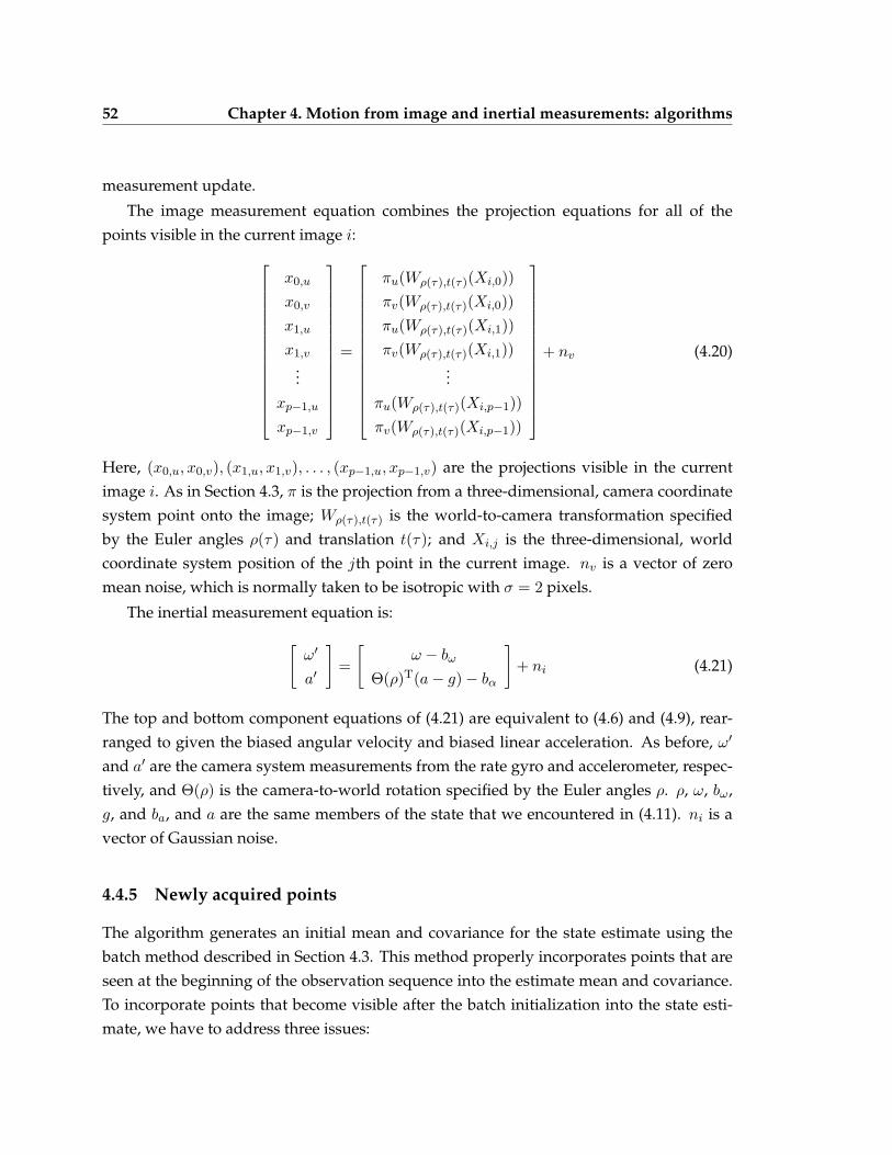
52 Chapter 4. Motion from image and inertial measurements: algorithms
measurement update.
The image measurement equation combines the projection equations for all of thepoints visible in the current image i:
x0,u
x0,v
x1,u
x1,v
...xp−1,u
xp−1,v
=
πu(Wρ(τ),t(τ)(Xi,0))πv(Wρ(τ),t(τ)(Xi,0))πu(Wρ(τ),t(τ)(Xi,1))πv(Wρ(τ),t(τ)(Xi,1))
...πu(Wρ(τ),t(τ)(Xi,p−1))πv(Wρ(τ),t(τ)(Xi,p−1))
+ nv (4.20)
Here, (x0,u, x0,v), (x1,u, x1,v), . . . , (xp−1,u, xp−1,v) are the projections visible in the currentimage i. As in Section 4.3, π is the projection from a three-dimensional, camera coordinatesystem point onto the image; Wρ(τ),t(τ) is the world-to-camera transformation specifiedby the Euler angles ρ(τ) and translation t(τ); and Xi,j is the three-dimensional, worldcoordinate system position of the jth point in the current image. nv is a vector of zeromean noise, which is normally taken to be isotropic with σ = 2 pixels.
The inertial measurement equation is:
[ω′
a′
]=
[ω − bω
Θ(ρ)T(a− g)− bα
]+ ni (4.21)
The top and bottom component equations of (4.21) are equivalent to (4.6) and (4.9), rear-ranged to given the biased angular velocity and biased linear acceleration. As before, ω′
and a′ are the camera system measurements from the rate gyro and accelerometer, respec-tively, and Θ(ρ) is the camera-to-world rotation specified by the Euler angles ρ. ρ, ω, bω,g, and ba, and a are the same members of the state that we encountered in (4.11). ni is avector of Gaussian noise.
4.4.5 Newly acquired points
The algorithm generates an initial mean and covariance for the state estimate using thebatch method described in Section 4.3. This method properly incorporates points that areseen at the beginning of the observation sequence into the estimate mean and covariance.To incorporate points that become visible after the batch initialization into the state esti-mate, we have to address three issues:
4.4. Recursive estimation 53
1. Determining which new points to incorporate into the state estimate.
2. Finding a mean for new points that are to be incorporated into the state estimate.
3. Finding a variance for new points that are to be incorporated into the state estimate,and the covariances that relate them to the estimates of the other state componentsand to the other new points.
This subsection describes the approach to each of these issues, with emphasis on the mostdifficult issue, correct computation of the variances and covariances.
To address the first issue, the incorporation of newly visible points into the state esti-mate is delayed until the point’s three-dimensional position can be computed accuratelyrelative to the camera positions from which it was visible, i.e., until its variance relativeto the most recent camera position is below some threshold. This is to prevent numeri-cal problems and reduce bias in the filter. The number of images required to achieve asufficiently low variance in the point’s position depends on the translation between theimages.
Finding a mean for a point that has become visible after the batch initialization isstraightforward. The camera positions estimated by the filter for the images in which thepoint was visible are used to triangulate the point’s position.
Determining the new state covariance matrix is more complex, and must consider thefollowing interrelated requirements:
1. The mean and covariance estimates produced by the recursive estimation shouldapproximate those produced by a batch estimation as closely as allowed by the choiceof the filter state and the filter’s Gaussian prior assumption. This requirement is afundamental design goal of recursive estimation algorithms, and requirements 2, 3,and 4 below are satisfied if this requirement is satisfied.
2. The state estimate distribution (i.e., mean and covariance) that results from the pointinitialization should not be too optimistic, which would weight the observationsused in the point initialization more than those used in subsequent measurementupdates, or too conservative, which would weight the observations used in the pointinitialization less than those used in subsequent measurement updates. This is im-portant to ensure that the resulting estimates will be consistent with all of the ob-servations, insofar as the observations allow. This also ensures that the availableobservations are best utilized, which is important in sequences where each point isonly visible in a short subsequence of the image sequence.
54 Chapter 4. Motion from image and inertial measurements: algorithms
3. The resulting filter should accurately estimate the covariances of the camera position,camera velocity, and point positions in the world coordinate system so that thesecan be monitored in critical applications. This is particularly important for long se-quences, in which these variances will necessarily increase with time as points enterand leave the camera’s field of view.
4. The variance of points relative to the current camera position, which is generallylower than the variance of the points relative to the world coordinate system, shouldbe accurately estimated. This is important if the output of the filter will be usedto generate image coordinate system priors for tracking the points in subsequentimages.
To satisfy these requirements as closely as possible, the method described by Smith, etal.[54] for integrating newly visible landmarks into extended Kalman filters in simultane-ous localization and mapping (SLAM) applications has been adapted. The motivation ofSmith, et al.’s method is to properly incorporate sensor coordinate system measurementsand covariances into global coordinate system estimates and covariances given the co-variance associated with the sensor position, and to allow the sensor coordinate systemmeasurement and covariance to be reextracted from the global coordinate system mea-surement and covariance. As described in subsection 2.4, SLAM applications typicallyuse active range sensors, which provide measurements of both the range and bearing (i.e.,the point’s full three-dimensional location) in the sensor’s coordinate system. In motionestimation from image measurements, only the bearing is available from any one sensormeasurement. The rest of this subsection briefly describes Smith, et al.’s method, describeshow it has been applied to the bearings-only case, and discusses the relative advantagesand disadvantages of this approach versus some possible alternative approaches.
Smith, et al.’s method operates as follows. Suppose that:
• x is the filter’s state estimate before the incorporation of the new point estimate, andthat C(x) is the covariance estimate for x produced by the most recent measurementupdate step
• zw is the world coordinate system point corresponding to the sensor coordinate sys-tem point zc
• g(x, zc) is the rigid transformation that maps zc to zw
• Gx and Gzc are the derivatives of g with respect to x and zc, respectively, evaluatedat the current estimates of x and zc
4.4. Recursive estimation 55
Then, Smith et al.’s method transforms the sensor coordinate system covariance C(zc) intoa world coordinate system covariance C(zw), and establishes a cross-covariance C(x, zw)between x and zw, using
C(zw) = GxC(x)GTx + GzcC(zc)GT
zc(4.22)
C(x, zw) = GxC(x) (4.23)
The new point can then be incorporated into the state estimate by augmenting x with zw,and C(x) with C(zw) and C(x, zw).
To adapt this method to the bearings-only case by assuming that the camera positionestimates corresponding to the initialization images in which the point was visible are cor-rect with respect to each other. Mean and covariance estimates for the point’s positionrelative to the most recent camera position can be computed under this assumption, effec-tively producing a “virtual range device” that can be used in Smith, et al.’s method. Themean and variance of this virtual device’s position with respect to the world coordinatesystem are that of the most recent camera position.
This method correctly accounts for the variances in the image observations used inthe point initialization and the estimated uncertainty in the current camera estimate, butnot for any relative error between the recent estimated camera positions. As a result, thismethod produces covariances that are quite close to those produced by a batch estimationif the relative error between the camera estimates is small, satisfying requirement 1 andrequirements 2, 3, and 4, which follow from it. However, in those cases where there is asignificant relative error between the recent camera estimates (e.g., because of point featuremistracking), the new point will be initialized with an overly optimistic covariance, andsubsequent state estimates will be contaminated by this error.
This approach is superior to two alternatives. In the first, camera system variancesfor the newly visible points are computed using the error variances associated with thepoints’ image feature observations, and rotated into the world coordinate system using thecurrent camera-to-world rotation estimate. This strategy correctly reflects the accuracy ofthe points’ estimated positions relative to the current camera position (requirement 4), butdoes not capture the potentially high error in the points’ estimated positions relative to theworld coordinate system (requirement 3). This potentially large error in the points’ worldcoordinate system position estimates is inevitable, since the error in the camera positionsused to estimate the features’ positions will grow large for long image sequences. Afterthese inadvertently low variances have been assigned to the points, all of the filter’s errorvariances will become corrupted, since subsequent camera positions will be estimated with
56 Chapter 4. Motion from image and inertial measurements: algorithms
respect to points that appear to have a low world coordinate system variances, and willtherefore be assigned low variances in turn (violating requirement 1).
In the second, fixed variances, the variances described in the previous paragraph, orsome other reasonable camera coordinate system variances are adopted, but inflated in anattempt to reflect the potential inaccuracy in the points’ estimated positions relative to theworld coordinate system. This strategy is poor for the following reasons. First, this strat-egy does not reflect the accuracy of the points’ estimated positions relative to the currentcamera position, which may be useful information, e.g., for tracking the point’s position insubsequent images (requirement 4). Second, for any fixed inflation factor, this choice alsomay not reflect the point’s inaccuracy in the world coordinate system, which may growarbitrarily large given long sequences (requirement 3). Third, this method effectively jetti-sons all of the information about the points’ positions provided by the points’ initial imagefeature observation variances, so the estimated three-dimensional point positions may be-come inconsistent with the initial views of the point (requirement 2).
As mentioned above, this adaption of Smith, Self, and Cheeseman method cannotmodel the relative errors between the successive camera position estimates that comprisethe “virtual range device”. An alternative approach that models the relative errors be-tween successive camera positions is the variable state dimension filter (VSDF) describedby McLauchlan[38]. The VSDF is a hybrid batch-recursive approach rather than a Kalmanfilter, so this modeling comes at the cost of increased computation. The batch method de-scribed in Section 4.3 could be adapted for hybrid batch-recursive operation within theVSDF framework. Within the Kalman filter framework described in this chapter, however,only the most recent camera position is included in the state. In this case, the adaptationof Smith, et al.’s method described in this section is recommended.
4.4.6 Lost points
To limit the filter state dimension as new points become visible and are added to the state,the recursive method removes the three-dimensional positions of points lost by the trackerfrom the state by removing the corresponding entries of the mean and covariance esti-mates, and leaving all other mean and covariance values unchanged. This is equivalent tomarginalizing over the removed point’s state components.
4.4.7 Image-only estimation
Section 5.6 describes both recursive image-and-inertial estimates and recursive image-only estimates. The recursive image-only algorithm is similar to the recursive image-and-
4.4. Recursive estimation 57
inertial algorithm described in this section, with the following differences:
• Only the camera rotation, the camera translation, and the three-dimensional posi-tions of the currently visible points are included in the state.
• The state propagation assumes slowly changing camera rotation and translation ratherthan slowly changing angular velocity and linear acceleration.
• The state estimate is initialized using the batch image-only algorithm rather than thebatch image-and-inertial algorithm.
• There is no inertial measurement update.
The image measurement update step, the method for incorporating newly visible points,and the policy for dropping lost points from the state are the same as those for the recursiveimage-and-inertial algorithm.
4.4.8 Discussion
As mentioned in subsection 4.4.5, a common goal of recursive algorithm design is to in-corporate measurements as they become available, while approximating the state meanand covariance estimates that would be produced by a batch algorithm given all of themeasurements at once. For instance, the recursive image-only algorithm described in sub-section 4.4.7 above produces estimates that closely match those of the batch image-onlyalgorithm described in subsection 2.10. This is particularly true as the time propagationvariances that specify how close we expect camera positions at adjacent times to be areallowed to grow, easing the assumption of motion smoothness, which the batch methoddoes not incorporate.
The batch and recursive image-and-inertial algorithms described in this chapter arenot as closely related in this way. For instance, the batch algorithm estimates the sensorposition only at the time of each image, while the recursive algorithm estimates the sensorposition at the time of each image and each inertial measurement.
More importantly, the multirate design of the recursive algorithm implicitly requiresthe assumption of smoothness in the angular velocity and linear acceleration across mea-surement times to exploit inertial and image measurements acquired at different times.Consider, for example, an inertial measurement followed by an image measurement. Ifthe angular velocity and linear acceleration time propagation variances are high, as re-quired in scenarios with erratic motion, then the state prior covariance that results fromthe time propagation between the inertial and image measurement times grows quickly
58 Chapter 4. Motion from image and inertial measurements: algorithms
and only loosely constrains the image measurement step estimate. So, the filter is free tochoose an estimate at the time of the image measurement that is quite different than thestate estimate that resulted from the inertial measurement step. On the other hand, motionsmoothness is not a critical assumption for combining measurements taken at differentimage times, as it is in the recursive image-only filter, because these estimates are relatedthrough the three-dimensional positions of the points observed at both times.
The batch algorithm, including the integration functions Iρ, Iv, and It that integrateinertial measurement between image times, neither requires nor exploits such an assump-tion, so the batch algorithm is stronger than the recursive algorithm in the presence oferratic motion. It appears that robustness to erratic motion is more valuable in practicethan the assumption of motion smoothness, and Tomasi and Kanade[56] drew a similarconclusion in the context of shape-from-motion. Increasing the robustness of the recursiveimage-and-inertial algorithm to erratic motion is a promising direction for future work.
Chapter 5
Motion from image and inertialmeasurements: experiments
5.1 Overview
Chapters 3 and Chapter 4 above describe the potential advantages of motion from om-nidirectional images and of motion from image and inertial measurements, respectively,and describe algorithms for exploiting these approaches. This chapter presents a suite ofexperiments in which sensor motion and other unknowns have been estimated using thealgorithms described in those chapters, with emphasis on motion from image and inertialmeasurements. The experiments aim both to evaluate the specific algorithms that havebeen developed in those chapters, and to establish some fundamental facts about motionestimation using these modalities.
This chapter is organized as follows. Section 5.2 gives an overview of four suites ofexperiments. The camera configuration, observations, and results for each of these foursuites are then described in detail in Sections 5.3-5.6.
As desribed in the introduction, motion estimation from omnidirectional images andmotion from image and inertial measurements are two of the four approaches for improv-ing motion estimation that this thesis investigates. Based in part on the results in thischapter, the conclusion in Chapter 8 contains some recommendations about the relativemerits of, and for exploiting, these different approaches.
59
60 Chapter 5. Motion from image and inertial measurements: experiments
5.2 Experiments overview
This section gives a high level overview of the experiments (subsection 5.2.1), a descrip-tion of the inertial sensor configuration (subsection 5.2.2), and the motion error metricsused to evaluate the accuracy of our estimates (subsection 5.2.3). The inertial sensor con-figuration and the motion error metrics are the same across the experiments described inthe subsequent sections.
5.2.1 The experiments
A high level overview of the experiments is as follows:
Perspective arm experiment. The sensor rig includes a perspective camera and theinertial sensors and is mounted on a robotic arm that undergoes a known, preprogrammedmotion. For each of the batch image-and-inertial, batch image-only, and recursive image-and-inertial algorithms, the estimation accuracy as the estimation parameters, the initialestimates, and the speed of the motion vary are explored.
Omnidirectional arm experiments. Three omnidirectional experiments were perform-ing by mounting the two omnidirectional cameras and inertial sensors on the same armused in the perspective arm experiment. Estimates were again generated using the batchimage-and-inertial, batch image-only, and recursive image-and-inertial algorithms. In eachexperiment the motion is similar to that in the perspective arm experiment, so the relativemerits of omnidirectional cameras and inertial sensors for motion estimation can be inves-tigated.
Perspective crane experiment. The sensor rig includes a conventional camera and theinertial sensors, and is mounted on the platform of a robotic crane that can translate withina workspace of about 10 m × 10 m × 5 m. An estimate was generated using the recursiveimage-and-inertial algorithm.
Perspective rover experiments. The sensor rig includes a conventional camera and theinertial sensors, and is mounted on a ground rover that traverses approximately 230 me-ters. Estimates were generated using the recursive image-only algorithm and the recursiveimage-and-inertial algorithm.
Figure 5.1 shows the overall organization of the suite of experiments in more detail.
5.2.2 Inertial sensors
As described in the previous sections, a promising approach to a robust system for motionestimation is to augment motion estimation from image measurements with data from
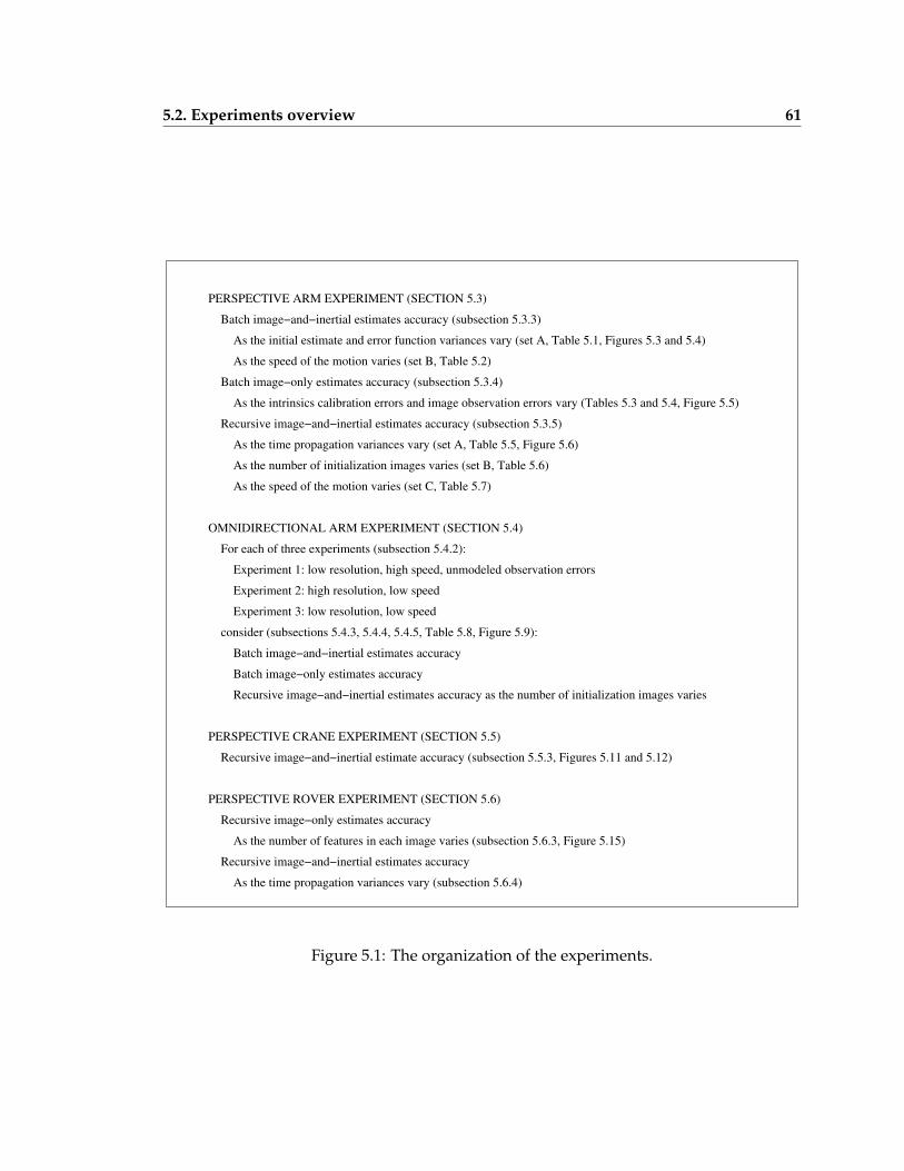
5.2. Experiments overview 61
PERSPECTIVE ARM EXPERIMENT (SECTION 5.3)
As the speed of the motion varies (set B, Table 5.2)
Batch image−only estimates accuracy (subsection 5.3.4)
Batch image−and−inertial estimates accuracy (subsection 5.3.3)
Recursive image−and−inertial estimates accuracy (subsection 5.3.5)
As the number of initialization images varies (set B, Table 5.6)
As the speed of the motion varies (set C, Table 5.7)
OMNIDIRECTIONAL ARM EXPERIMENT (SECTION 5.4)
For each of three experiments (subsection 5.4.2):
Experiment 1: low resolution, high speed, unmodeled observation errors
Experiment 2: high resolution, low speed
Experiment 3: low resolution, low speed
Batch image−and−inertial estimates accuracy
Batch image−only estimates accuracy
Recursive image−and−inertial estimates accuracy as the number of initialization images varies
PERSPECTIVE CRANE EXPERIMENT (SECTION 5.5)
As the intrinsics calibration errors and image observation errors vary (Tables 5.3 and 5.4, Figure 5.5)
As the initial estimate and error function variances vary (set A, Table 5.1, Figures 5.3 and 5.4)
PERSPECTIVE ROVER EXPERIMENT (SECTION 5.6)
Recursive image−only estimates accuracy
Recursive image−and−inertial estimates accuracy
As the time propagation variances vary (subsection 5.6.4)
As the time propagation variances vary (set A, Table 5.5, Figure 5.6)
consider (subsections 5.4.3, 5.4.4, 5.4.5, Table 5.8, Figure 5.9):
As the number of features in each image varies (subsection 5.6.3, Figure 5.15)
Recursive image−and−inertial estimate accuracy (subsection 5.5.3, Figures 5.11 and 5.12)
Figure 5.1: The organization of the experiments.
62 Chapter 5. Motion from image and inertial measurements: experiments
small, low-cost inertial sensors. To this end, the same configuration of inertial sensors hasbeen used in all of the experiments, consisting of:
• Three single-axis, orthogonally mounted CRS04 rate gyros from Silicon Sensing Sys-tems, which measure up to ±150 degrees per second. Each of these gyros has ap-proximate dimensions 1 cm × 3 cm × 3 cm, weighs 12 gm, and has a single unit costof approximately $300.
• A Crossbow CXL04LP3 three degree of freedom accelerometer, which measures upto ±4 g. This accelerometer has approximate dimensions 2 cm × 4.75 cm × 2.5 cm,weighs 46 gm, and has a single unit cost of approximately $300.
The voltages from the rate gyros and the accelerometer were captured at 200 Hz using twoseparate Crossbow CXLDK boards.
The three gyro voltage-to-rate calibrations were determined using a turntable witha known rotational rate. The accelerometer voltage-to-acceleration calibration was per-formed using a field calibration that accounts for non-orthogonality between the individ-ual x, y, and z accelerometers. The gyro and accelerometer measurement error varianceswere found by sampling the sensors while they were kept stationary. The fixed gyro-to-camera and accelerometer-to-camera rotations differed between experiments but in eachcase were assumed known from the mechanical specifications of the mounts.
5.2.3 Motion error metrics
The simultaneous estimation of camera motion and scene structure from images alonerecovers estimates only up to a scaled rigid transformation. That is, applying the samescaling and rigid transformation to all of the camera and point estimates produces new es-timates that explain the observed data as well as the original estimates. With the incorpo-ration of accelerometer data, it is possible to recover the global scale and two componentsof the absolute rotation, but with inexpensive accelerometers will likely be only roughlycorrect.
Therefore, the recovered estimates have been transformed into the ground truth coor-dinate system using a scaled rigid transformation before computing motion rotation andtranslation errors. This transformation has the form
tg = sRte + t (5.1)
where tg and te are a camera translation in the ground truth and estimate coordinate sys-tems, respectively, and s, R, and t are the scale, rotation, and translation of the scaled rigid
5.3. Perspective arm experiment 63
transformation.
The scaled rigid transformation that best aligns the estimated camera translations withthe ground truth translations, which can be found in closed form using the absolute orien-tation method described by Horn[28], has been used. An alternative is to align the estimateof the initial camera position with the ground truth initial camera position. However, thisapproach will not accurately capture the global accuracy of a motion estimate.
The reported rotation errors are the absolute rotation angle that aligns the estimated,transformed three-dimensional camera rotation with the ground truth rotation. This an-gle is the angle component of the angle-axis representation of the relative rotation. Thereported translation errors are the distance in three-space between the estimated, trans-formed camera translation and the ground truth camera translations. For both rotationand translation, average and maximum errors are reported.
The error in global scale between the estimated and ground truth motion is reported.Specifically, the global scale is, as a percentage:
scale error = 1/s− 1 (5.2)
where s is the transformation scale in (5.1). So, the scale error is greater than 0 if the scaleof the estimated motion is larger than that of the ground truth motion, and less than 0otherwise.
5.3 Perspective arm experiment
In the first experiment a perspective camera and the inertial sensors were mounted on arobotic arm to produce image and inertial observations from a known motion. The re-sulting observation sequence and ground truth motion information were used to investi-gate the relative performance of the batch image-and-inertial, batch image-only, and recur-sive image-and-inertial algorithms, as the estimation parameters, initial estimates, and thespeed of the motion varied.
Subsections 5.3.1 and 5.3.2 below describe the sensor configuration and observations,respectively, for this experiment. Subsections 5.3.3, 5.3.4, and 5.3.5 describe the estimatesproduced by the batch image-and-inertial, batch image-only, and recursive image-and-inertial algorithms for from these observations. Because these sections include a largenumber of estimates, subsection 5.3.7 includes a concise summary of the key results.
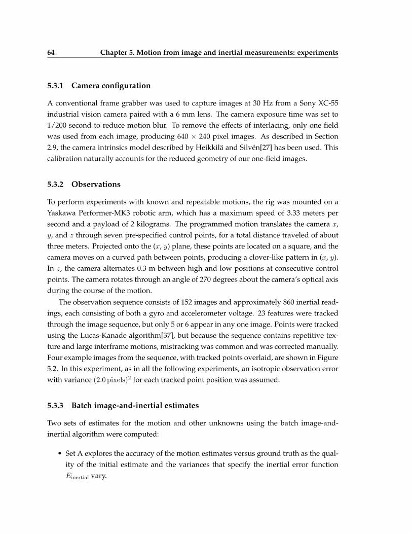
64 Chapter 5. Motion from image and inertial measurements: experiments
5.3.1 Camera configuration
A conventional frame grabber was used to capture images at 30 Hz from a Sony XC-55industrial vision camera paired with a 6 mm lens. The camera exposure time was set to1/200 second to reduce motion blur. To remove the effects of interlacing, only one fieldwas used from each image, producing 640 × 240 pixel images. As described in Section2.9, the camera intrinsics model described by Heikkila and Silven[27] has been used. Thiscalibration naturally accounts for the reduced geometry of our one-field images.
5.3.2 Observations
To perform experiments with known and repeatable motions, the rig was mounted on aYaskawa Performer-MK3 robotic arm, which has a maximum speed of 3.33 meters persecond and a payload of 2 kilograms. The programmed motion translates the camera x,y, and z through seven pre-specified control points, for a total distance traveled of aboutthree meters. Projected onto the (x, y) plane, these points are located on a square, and thecamera moves on a curved path between points, producing a clover-like pattern in (x, y).In z, the camera alternates 0.3 m between high and low positions at consecutive controlpoints. The camera rotates through an angle of 270 degrees about the camera’s optical axisduring the course of the motion.
The observation sequence consists of 152 images and approximately 860 inertial read-ings, each consisting of both a gyro and accelerometer voltage. 23 features were trackedthrough the image sequence, but only 5 or 6 appear in any one image. Points were trackedusing the Lucas-Kanade algorithm[37], but because the sequence contains repetitive tex-ture and large interframe motions, mistracking was common and was corrected manually.Four example images from the sequence, with tracked points overlaid, are shown in Figure5.2. In this experiment, as in all the following experiments, an isotropic observation errorwith variance (2.0 pixels)2 for each tracked point position was assumed.
5.3.3 Batch image-and-inertial estimates
Two sets of estimates for the motion and other unknowns using the batch image-and-inertial algorithm were computed:
• Set A explores the accuracy of the motion estimates versus ground truth as the qual-ity of the initial estimate and the variances that specify the inertial error functionEinertial vary.
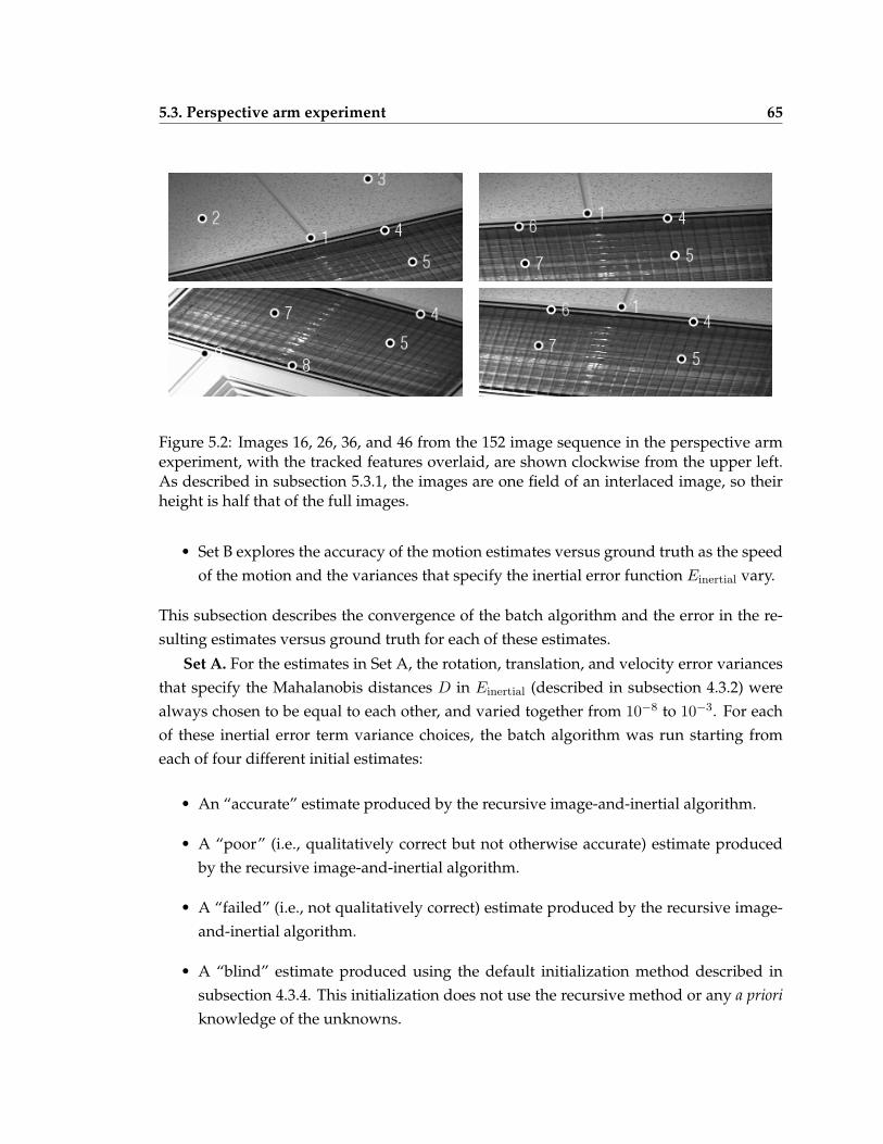
5.3. Perspective arm experiment 65
Figure 5.2: Images 16, 26, 36, and 46 from the 152 image sequence in the perspective armexperiment, with the tracked features overlaid, are shown clockwise from the upper left.As described in subsection 5.3.1, the images are one field of an interlaced image, so theirheight is half that of the full images.
• Set B explores the accuracy of the motion estimates versus ground truth as the speedof the motion and the variances that specify the inertial error function Einertial vary.
This subsection describes the convergence of the batch algorithm and the error in the re-sulting estimates versus ground truth for each of these estimates.
Set A. For the estimates in Set A, the rotation, translation, and velocity error variancesthat specify the Mahalanobis distances D in Einertial (described in subsection 4.3.2) werealways chosen to be equal to each other, and varied together from 10−8 to 10−3. For eachof these inertial error term variance choices, the batch algorithm was run starting fromeach of four different initial estimates:
• An “accurate” estimate produced by the recursive image-and-inertial algorithm.
• A “poor” (i.e., qualitatively correct but not otherwise accurate) estimate producedby the recursive image-and-inertial algorithm.
• A “failed” (i.e., not qualitatively correct) estimate produced by the recursive image-and-inertial algorithm.
• A “blind” estimate produced using the default initialization method described insubsection 4.3.4. This initialization does not use the recursive method or any a prioriknowledge of the unknowns.
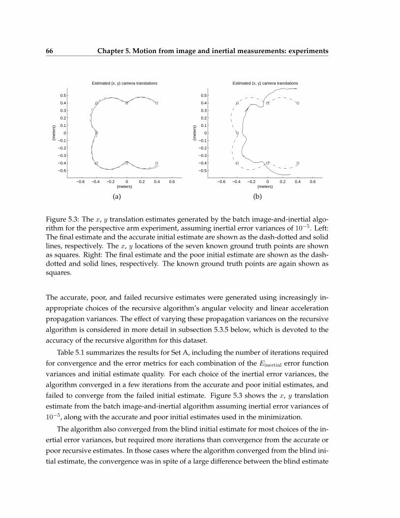
66 Chapter 5. Motion from image and inertial measurements: experiments
−0.6 −0.4 −0.2 0 0.2 0.4 0.6
−0.5
−0.4
−0.3
−0.2
−0.1
0
0.1
0.2
0.3
0.4
0.5
Estimated (x, y) camera translations
(meters)
(met
ers)
−0.6 −0.4 −0.2 0 0.2 0.4 0.6
−0.5
−0.4
−0.3
−0.2
−0.1
0
0.1
0.2
0.3
0.4
0.5
Estimated (x, y) camera translations
(meters)
(met
ers)
(a) (b)
Figure 5.3: The x, y translation estimates generated by the batch image-and-inertial algo-rithm for the perspective arm experiment, assuming inertial error variances of 10−5. Left:The final estimate and the accurate initial estimate are shown as the dash-dotted and solidlines, respectively. The x, y locations of the seven known ground truth points are shownas squares. Right: The final estimate and the poor initial estimate are shown as the dash-dotted and solid lines, respectively. The known ground truth points are again shown assquares.
The accurate, poor, and failed recursive estimates were generated using increasingly in-appropriate choices of the recursive algorithm’s angular velocity and linear accelerationpropagation variances. The effect of varying these propagation variances on the recursivealgorithm is considered in more detail in subsection 5.3.5 below, which is devoted to theaccuracy of the recursive algorithm for this dataset.
Table 5.1 summarizes the results for Set A, including the number of iterations requiredfor convergence and the error metrics for each combination of the Einertial error functionvariances and initial estimate quality. For each choice of the inertial error variances, thealgorithm converged in a few iterations from the accurate and poor initial estimates, andfailed to converge from the failed initial estimate. Figure 5.3 shows the x, y translationestimate from the batch image-and-inertial algorithm assuming inertial error variances of10−5, along with the accurate and poor initial estimates used in the minimization.
The algorithm also converged from the blind initial estimate for most choices of the in-ertial error variances, but required more iterations than convergence from the accurate orpoor recursive estimates. In those cases where the algorithm converged from the blind ini-tial estimate, the convergence was in spite of a large difference between the blind estimate
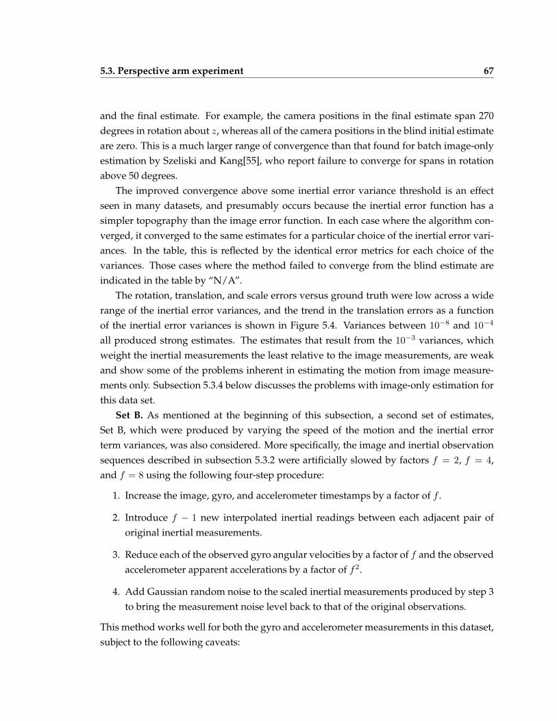
5.3. Perspective arm experiment 67
and the final estimate. For example, the camera positions in the final estimate span 270degrees in rotation about z, whereas all of the camera positions in the blind initial estimateare zero. This is a much larger range of convergence than that found for batch image-onlyestimation by Szeliski and Kang[55], who report failure to converge for spans in rotationabove 50 degrees.
The improved convergence above some inertial error variance threshold is an effectseen in many datasets, and presumably occurs because the inertial error function has asimpler topography than the image error function. In each case where the algorithm con-verged, it converged to the same estimates for a particular choice of the inertial error vari-ances. In the table, this is reflected by the identical error metrics for each choice of thevariances. Those cases where the method failed to converge from the blind estimate areindicated in the table by “N/A”.
The rotation, translation, and scale errors versus ground truth were low across a widerange of the inertial error variances, and the trend in the translation errors as a functionof the inertial error variances is shown in Figure 5.4. Variances between 10−8 and 10−4
all produced strong estimates. The estimates that result from the 10−3 variances, whichweight the inertial measurements the least relative to the image measurements, are weakand show some of the problems inherent in estimating the motion from image measure-ments only. Subsection 5.3.4 below discusses the problems with image-only estimation forthis data set.
Set B. As mentioned at the beginning of this subsection, a second set of estimates,Set B, which were produced by varying the speed of the motion and the inertial errorterm variances, was also considered. More specifically, the image and inertial observationsequences described in subsection 5.3.2 were artificially slowed by factors f = 2, f = 4,and f = 8 using the following four-step procedure:
1. Increase the image, gyro, and accelerometer timestamps by a factor of f .
2. Introduce f − 1 new interpolated inertial readings between each adjacent pair oforiginal inertial measurements.
3. Reduce each of the observed gyro angular velocities by a factor of f and the observedaccelerometer apparent accelerations by a factor of f2.
4. Add Gaussian random noise to the scaled inertial measurements produced by step 3to bring the measurement noise level back to that of the original observations.
This method works well for both the gyro and accelerometer measurements in this dataset,subject to the following caveats:
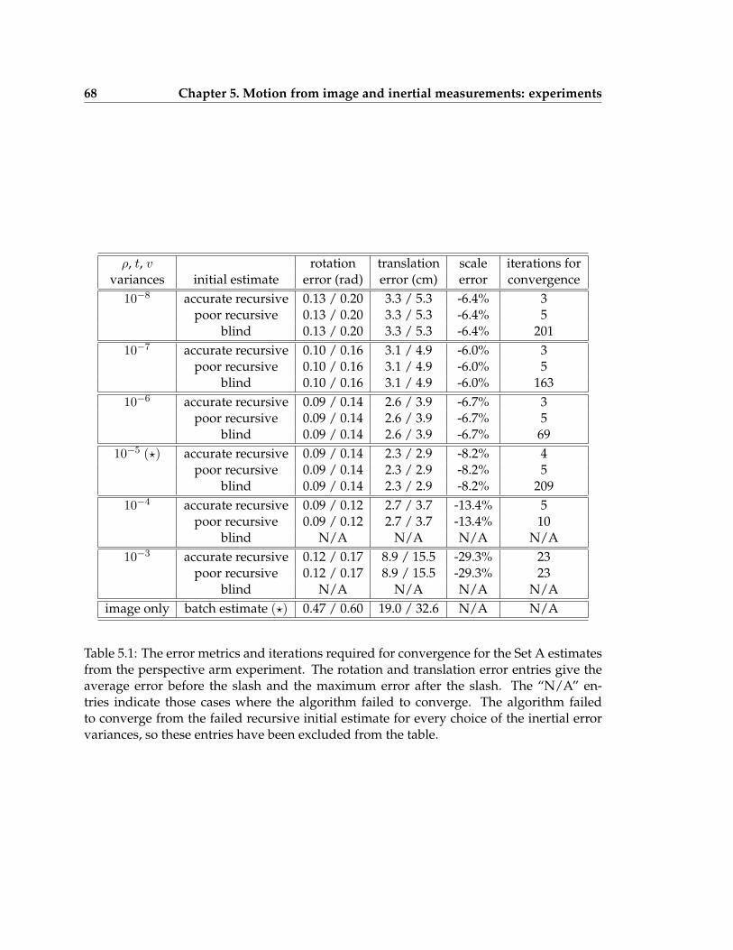
68 Chapter 5. Motion from image and inertial measurements: experiments
ρ, t, v rotation translation scale iterations forvariances initial estimate error (rad) error (cm) error convergence
10−8 accurate recursive 0.13 / 0.20 3.3 / 5.3 -6.4% 3poor recursive 0.13 / 0.20 3.3 / 5.3 -6.4% 5
blind 0.13 / 0.20 3.3 / 5.3 -6.4% 20110−7 accurate recursive 0.10 / 0.16 3.1 / 4.9 -6.0% 3
poor recursive 0.10 / 0.16 3.1 / 4.9 -6.0% 5blind 0.10 / 0.16 3.1 / 4.9 -6.0% 163
10−6 accurate recursive 0.09 / 0.14 2.6 / 3.9 -6.7% 3poor recursive 0.09 / 0.14 2.6 / 3.9 -6.7% 5
blind 0.09 / 0.14 2.6 / 3.9 -6.7% 6910−5 (?) accurate recursive 0.09 / 0.14 2.3 / 2.9 -8.2% 4
poor recursive 0.09 / 0.14 2.3 / 2.9 -8.2% 5blind 0.09 / 0.14 2.3 / 2.9 -8.2% 209
10−4 accurate recursive 0.09 / 0.12 2.7 / 3.7 -13.4% 5poor recursive 0.09 / 0.12 2.7 / 3.7 -13.4% 10
blind N/A N/A N/A N/A10−3 accurate recursive 0.12 / 0.17 8.9 / 15.5 -29.3% 23
poor recursive 0.12 / 0.17 8.9 / 15.5 -29.3% 23blind N/A N/A N/A N/A
image only batch estimate (?) 0.47 / 0.60 19.0 / 32.6 N/A N/A
Table 5.1: The error metrics and iterations required for convergence for the Set A estimatesfrom the perspective arm experiment. The rotation and translation error entries give theaverage error before the slash and the maximum error after the slash. The “N/A” en-tries indicate those cases where the algorithm failed to converge. The algorithm failedto converge from the failed recursive initial estimate for every choice of the inertial errorvariances, so these entries have been excluded from the table.
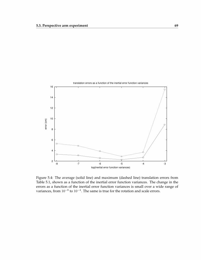
5.3. Perspective arm experiment 69
2
4
6
8
10
12
14
16
-8 -7 -6 -5 -4 -3
erro
r (cm
)
log(inertial error function variances)
translation errors as a function of the inertial error function variances
Figure 5.4: The average (solid line) and maximum (dashed line) translation errors fromTable 5.1, shown as a function of the inertial error function variances. The change in theerrors as a function of the inertial error function variances is small over a wide range ofvariances, from 10−8 to 10−4. The same is true for the rotation and scale errors.
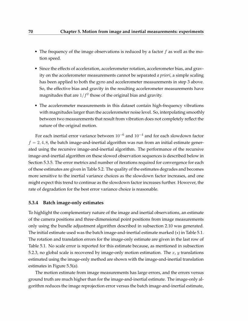
70 Chapter 5. Motion from image and inertial measurements: experiments
• The frequency of the image observations is reduced by a factor f as well as the mo-tion speed.
• Since the effects of acceleration, accelerometer rotation, accelerometer bias, and grav-ity on the accelerometer measurements cannot be separated a priori, a simple scalinghas been applied to both the gyro and accelerometer measurements in step 3 above.So, the effective bias and gravity in the resulting accelerometer measurements havemagnitudes that are 1/f2 those of the original bias and gravity.
• The accelerometer measurements in this dataset contain high-frequency vibrationswith magnitudes larger than the accelerometer noise level. So, interpolating smoothlybetween two measurements that result from vibration does not completely reflect thenature of the original motion.
For each inertial error variance between 10−6 and 10−4 and for each slowdown factorf = 2, 4, 8, the batch image-and-inertial algorithm was run from an initial estimate gener-ated using the recursive image-and-inertial algorithm. The performance of the recursiveimage-and-inertial algorithm on these slowed observation sequences is described below inSection 5.3.5. The error metrics and number of iterations required for convergence for eachof these estimates are given in Table 5.2. The quality of the estimates degrades and becomesmore sensitive to the inertial variance choices as the slowdown factor increases, and onemight expect this trend to continue as the slowdown factor increases further. However, therate of degradation for the best error variance choice is reasonable.
5.3.4 Batch image-only estimates
To highlight the complementary nature of the image and inertial observations, an estimateof the camera positions and three-dimensional point positions from image measurementsonly using the bundle adjustment algorithm described in subsection 2.10 was generated.The initial estimate used was the batch image-and-inertial estimate marked (?) in Table 5.1.The rotation and translation errors for the image-only estimate are given in the last row ofTable 5.1. No scale error is reported for this estimate because, as mentioned in subsection5.2.3, no global scale is recovered by image-only motion estimation. The x, y translationsestimated using the image-only method are shown with the image-and-inertial translationestimates in Figure 5.5(a).
The motion estimate from image measurements has large errors, and the errors versusground truth are much higher than for the image-and-inertial estimate. The image-only al-gorithm reduces the image reprojection error versus the batch image-and-inertial estimate,
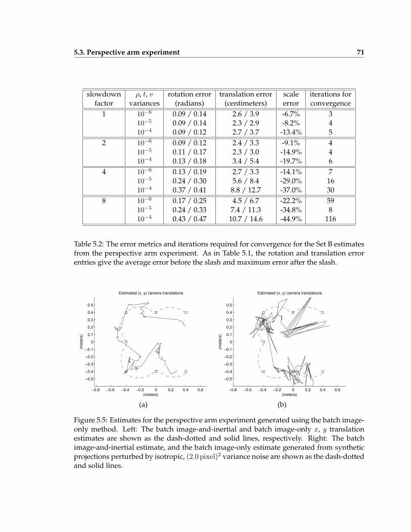
5.3. Perspective arm experiment 71
slowdown ρ, t, v rotation error translation error scale iterations forfactor variances (radians) (centimeters) error convergence
1 10−6 0.09 / 0.14 2.6 / 3.9 -6.7% 310−5 0.09 / 0.14 2.3 / 2.9 -8.2% 410−4 0.09 / 0.12 2.7 / 3.7 -13.4% 5
2 10−6 0.09 / 0.12 2.4 / 3.3 -9.1% 410−5 0.11 / 0.17 2.3 / 3.0 -14.9% 410−4 0.13 / 0.18 3.4 / 5.4 -19.7% 6
4 10−6 0.13 / 0.19 2.7 / 3.3 -14.1% 710−5 0.24 / 0.30 5.6 / 8.4 -29.0% 1610−4 0.37 / 0.41 8.8 / 12.7 -37.0% 30
8 10−6 0.17 / 0.25 4.5 / 6.7 -22.2% 5910−5 0.24 / 0.33 7.4 / 11.3 -34.8% 810−4 0.43 / 0.47 10.7 / 14.6 -44.9% 116
Table 5.2: The error metrics and iterations required for convergence for the Set B estimatesfrom the perspective arm experiment. As in Table 5.1, the rotation and translation errorentries give the average error before the slash and maximum error after the slash.
−0.8 −0.6 −0.4 −0.2 0 0.2 0.4 0.6
−0.5
−0.4
−0.3
−0.2
−0.1
0
0.1
0.2
0.3
0.4
0.5
Estimated (x, y) camera translations
(meters)
(met
ers)
−0.8 −0.6 −0.4 −0.2 0 0.2 0.4 0.6
−0.5
−0.4
−0.3
−0.2
−0.1
0
0.1
0.2
0.3
0.4
0.5
Estimated (x, y) camera translations
(meters)
(met
ers)
(a) (b)
Figure 5.5: Estimates for the perspective arm experiment generated using the batch image-only method. Left: The batch image-and-inertial and batch image-only x, y translationestimates are shown as the dash-dotted and solid lines, respectively. Right: The batchimage-and-inertial estimate, and the batch image-only estimate generated from syntheticprojections perturbed by isotropic, (2.0 pixel)2 variance noise are shown as the dash-dottedand solid lines.
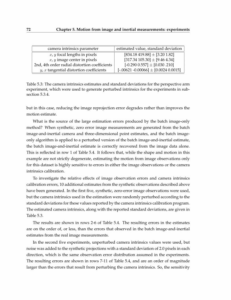
72 Chapter 5. Motion from image and inertial measurements: experiments
camera intrinsics parameter estimated value, standard deviationx, y focal lengths in pixels [834.18 419.88] ± [3.20 1.82]x, y image center in pixels [317.34 105.30] ± [9.46 4.34]
2nd, 4th order radial distortion coefficients [-0.290 0.557] ± [0.030 .210]y, x tangential distortion coefficients [-.00621 -0.00066] ± [0.0024 0.0015]
Table 5.3: The camera intrinsics estimates and standard deviations for the perspective armexperiment, which were used to generate perturbed intrinsics for the experiments in sub-section 5.3.4.
but in this case, reducing the image reprojection error degrades rather than improves themotion estimate.
What is the source of the large estimation errors produced by the batch image-onlymethod? When synthetic, zero error image measurements are generated from the batchimage-and-inertial camera and three-dimensional point estimates, and the batch image-only algorithm is applied to a perturbed version of the batch image-and-inertial estimate,the batch image-and-inertial estimate is correctly recovered from the image data alone.This is reflected in row 1 of Table 5.4. It follows that, while the shape and motion in thisexample are not strictly degenerate, estimating the motion from image observations onlyfor this dataset is highly sensitive to errors in either the image observations or the cameraintrinsics calibration.
To investigate the relative effects of image observation errors and camera intrinsicscalibration errors, 10 additional estimates from the synthetic observations described abovehave been generated. In the first five, synthetic, zero-error image observations were used,but the camera intrinsics used in the estimation were randomly perturbed according to thestandard deviations for these values reported by the camera intrinsics calibration program.The estimated camera intrinsics, along with the reported standard deviations, are given inTable 5.3.
The results are shown in rows 2-6 of Table 5.4. The resulting errors in the estimatesare on the order of, or less, than the errors that observed in the batch image-and-inertialestimates from the real image measurements.
In the second five experiments, unperturbed camera intrinsics values were used, butnoise was added to the synthetic projections with a standard deviation of 2.0 pixels in eachdirection, which is the same observation error distribution assumed in the experiments.The resulting errors are shown in rows 7-11 of Table 5.4, and are an order of magnitudelarger than the errors that result from perturbing the camera intrinsics. So, the sensitivity
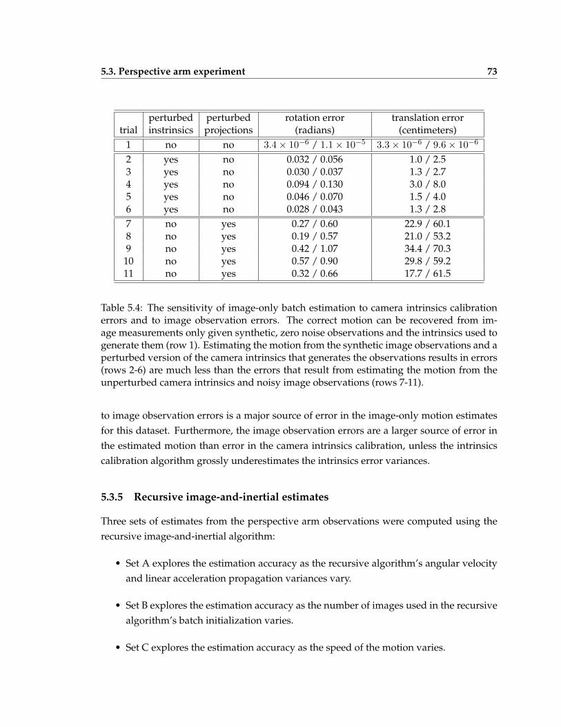
5.3. Perspective arm experiment 73
perturbed perturbed rotation error translation errortrial instrinsics projections (radians) (centimeters)
1 no no 3.4× 10⁻⁶ / 1.1× 10⁻⁵ 3.3× 10⁻⁶ / 9.6× 10⁻⁶
2 yes no 0.032 / 0.056 1.0 / 2.53 yes no 0.030 / 0.037 1.3 / 2.74 yes no 0.094 / 0.130 3.0 / 8.05 yes no 0.046 / 0.070 1.5 / 4.06 yes no 0.028 / 0.043 1.3 / 2.87 no yes 0.27 / 0.60 22.9 / 60.18 no yes 0.19 / 0.57 21.0 / 53.29 no yes 0.42 / 1.07 34.4 / 70.310 no yes 0.57 / 0.90 29.8 / 59.211 no yes 0.32 / 0.66 17.7 / 61.5
Table 5.4: The sensitivity of image-only batch estimation to camera intrinsics calibrationerrors and to image observation errors. The correct motion can be recovered from im-age measurements only given synthetic, zero noise observations and the intrinsics used togenerate them (row 1). Estimating the motion from the synthetic image observations and aperturbed version of the camera intrinsics that generates the observations results in errors(rows 2-6) are much less than the errors that result from estimating the motion from theunperturbed camera intrinsics and noisy image observations (rows 7-11).
to image observation errors is a major source of error in the image-only motion estimatesfor this dataset. Furthermore, the image observation errors are a larger source of error inthe estimated motion than error in the camera intrinsics calibration, unless the intrinsicscalibration algorithm grossly underestimates the intrinsics error variances.
5.3.5 Recursive image-and-inertial estimates
Three sets of estimates from the perspective arm observations were computed using therecursive image-and-inertial algorithm:
• Set A explores the estimation accuracy as the recursive algorithm’s angular velocityand linear acceleration propagation variances vary.
• Set B explores the estimation accuracy as the number of images used in the recursivealgorithm’s batch initialization varies.
• Set C explores the estimation accuracy as the speed of the motion varies.
74 Chapter 5. Motion from image and inertial measurements: experiments
Set A. 25 estimates were computed using the recursive image-and-inertial algorithm,and:
• varying the angular velocity propagation variance from (10−2 radians/s)2/s to(106 radians/s)2/s
• varying the linear acceleration propagation variance from (10−2 m/s2)2/s to(106 m/s2)2/s.
Guided by the batch algorithm results in Table 5.1, rotation, translation, and velocity er-ror variances of 10−5 have been adopted for the batch initialization in each case, and thebatch initialization uses 40 images in each case. The gyro and accelerometer measurementsvariances are from the sensor calibration described in subsection 5.2.2.
The results are summarized in Table 5.5 and Figure 5.6. Generally, the estimates aregood if the angular velocity variance is 102 or less and if the linear acceleration is 100 orgreater. If the linear acceleration is less than 100, then due to the strong accelerations inthe motion, the filter is unable to track the changes in linear acceleration. Of the variancestests, a angular velocity variance of 10−2 and a linear acceleration variance of 104 providethe best estimate, so these propagation variances have been adopted in sets B and C below.
Set B. 5 estimates were computed using the recursive image-and-inertial algorithmvarying the number of batch initialization images from 20 to 60. As in set A above, rota-tion, translation, and velocity error variances of 10−5 were used for the batch initialization,and based on the experiments in Set A above, angular velocity and linear accelerationpropagation variances of 10−2 and 104 respectively have been used.
The results are summarized in Table 5.6. The quality of the estimates degrades as thenumber of initialization images goes down. In particular, initializing from only 20 imagesproduces a poor recursive estimate for this dataset.
Set C. To investigate the robustness of the recursive method to changes in the overallspeed of the motion, 3 additional estimates were computed using the recursive image-and-inertial algorithm on the artificially slowed observation sequences described in subsection5.3.3 above. As in Set A, the batch initialization uses 40 images and 10−5 for the inertialerror variances. Based on the results from Set A, 10−2 and 104 have again been adopted asthe angular velocity and linear acceleration propagation variances, respectively.
The results are summarized in Table 5.7 below. As one might expect, the rotation andtranslation errors are slightly worse for the recursive algorithm than for the batch algo-rithm. However, their degradation as the overall motion speed and frequency of the imagemeasurements decrease is reasonable, and comparable to that of the batch algorithm.
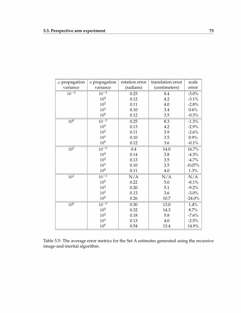
5.3. Perspective arm experiment 75
ω propagation a propagation rotation error translation error scalevariance variance (radians) (centimeters) error
10−2 10−2 0.25 8.4 -3.0%100 0.12 4.2 -3.1%102 0.11 4.0 -2.8%104 0.10 3.4 0.6%106 0.12 3.5 -0.3%
100 10−2 0.25 8.3 -1.3%100 0.13 4.2 -2.9%102 0.11 3.9 -2.6%104 0.10 3.5 0.9%106 0.12 3.6 -0.1%
102 10−2 0.4 14.0 16.7%100 0.14 3.8 -4.3%102 0.13 3.5 -4.7%104 0.10 3.5 -0.07%106 0.11 4.0 1.3%
104 10−2 N/A N/A N/A100 0.22 5.0 -8.1%102 0.20 5.1 -9.2%104 0.13 3.6 -3.0%106 0.26 10.7 -24.0%
106 10−2 0.30 13.0 1.4%100 0.32 14.3 8.7%102 0.18 5.8 -7.6%104 0.13 4.0 -2.5%106 0.54 13.4 14.9%
Table 5.5: The average error metrics for the Set A estimates generated using the recursiveimage-and-inertial algorithm.
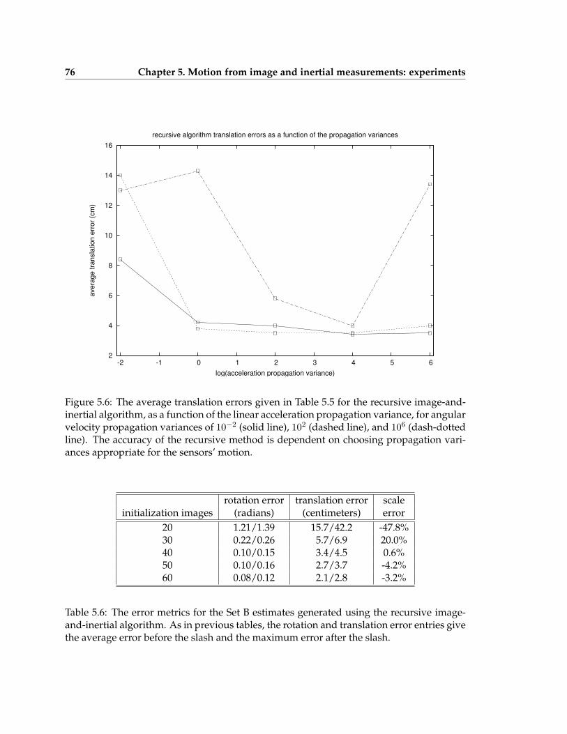
76 Chapter 5. Motion from image and inertial measurements: experiments
2
4
6
8
10
12
14
16
-2 -1 0 1 2 3 4 5 6
aver
age
trans
latio
n er
ror (
cm)
log(acceleration propagation variance)
recursive algorithm translation errors as a function of the propagation variances
Figure 5.6: The average translation errors given in Table 5.5 for the recursive image-and-inertial algorithm, as a function of the linear acceleration propagation variance, for angularvelocity propagation variances of 10−2 (solid line), 102 (dashed line), and 106 (dash-dottedline). The accuracy of the recursive method is dependent on choosing propagation vari-ances appropriate for the sensors’ motion.
rotation error translation error scaleinitialization images (radians) (centimeters) error
20 1.21/1.39 15.7/42.2 -47.8%30 0.22/0.26 5.7/6.9 20.0%40 0.10/0.15 3.4/4.5 0.6%50 0.10/0.16 2.7/3.7 -4.2%60 0.08/0.12 2.1/2.8 -3.2%
Table 5.6: The error metrics for the Set B estimates generated using the recursive image-and-inertial algorithm. As in previous tables, the rotation and translation error entries givethe average error before the slash and the maximum error after the slash.
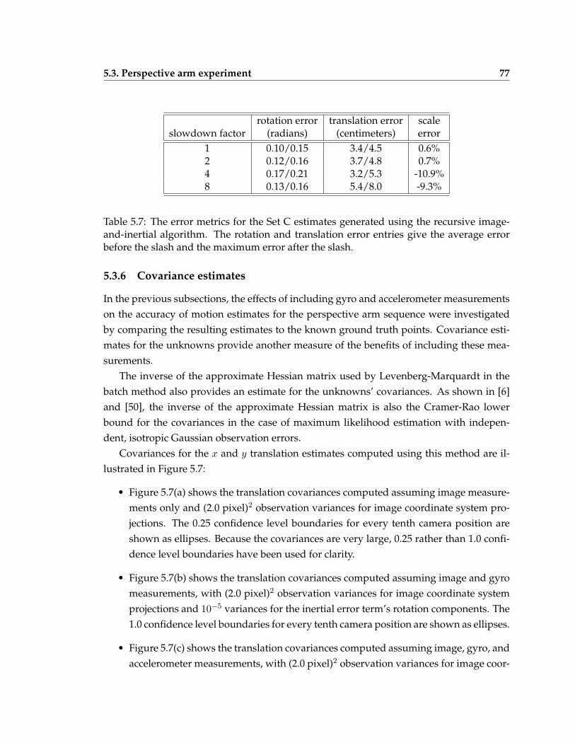
5.3. Perspective arm experiment 77
rotation error translation error scaleslowdown factor (radians) (centimeters) error
1 0.10/0.15 3.4/4.5 0.6%2 0.12/0.16 3.7/4.8 0.7%4 0.17/0.21 3.2/5.3 -10.9%8 0.13/0.16 5.4/8.0 -9.3%
Table 5.7: The error metrics for the Set C estimates generated using the recursive image-and-inertial algorithm. The rotation and translation error entries give the average errorbefore the slash and the maximum error after the slash.
5.3.6 Covariance estimates
In the previous subsections, the effects of including gyro and accelerometer measurementson the accuracy of motion estimates for the perspective arm sequence were investigatedby comparing the resulting estimates to the known ground truth points. Covariance esti-mates for the unknowns provide another measure of the benefits of including these mea-surements.
The inverse of the approximate Hessian matrix used by Levenberg-Marquardt in thebatch method also provides an estimate for the unknowns’ covariances. As shown in [6]and [50], the inverse of the approximate Hessian matrix is also the Cramer-Rao lowerbound for the covariances in the case of maximum likelihood estimation with indepen-dent, isotropic Gaussian observation errors.
Covariances for the x and y translation estimates computed using this method are il-lustrated in Figure 5.7:
• Figure 5.7(a) shows the translation covariances computed assuming image measure-ments only and (2.0 pixel)2 observation variances for image coordinate system pro-jections. The 0.25 confidence level boundaries for every tenth camera position areshown as ellipses. Because the covariances are very large, 0.25 rather than 1.0 confi-dence level boundaries have been used for clarity.
• Figure 5.7(b) shows the translation covariances computed assuming image and gyromeasurements, with (2.0 pixel)2 observation variances for image coordinate systemprojections and 10−5 variances for the inertial error term’s rotation components. The1.0 confidence level boundaries for every tenth camera position are shown as ellipses.
• Figure 5.7(c) shows the translation covariances computed assuming image, gyro, andaccelerometer measurements, with (2.0 pixel)2 observation variances for image coor-
78 Chapter 5. Motion from image and inertial measurements: experiments
dinate system projections and 10−5 variances for the inertial error term’s rotation,velocity, and translation components. The 1.0 confidence level boundaries for everytenth camera position are shown as ellipses.
In each case, the covariances were computed using the “?” estimate described in the Ta-ble 5.1. The increasing benefits of adding gyro and then accelerometer measurements arereflected in the covariance estimates.
5.3.7 Summary
The experiments in this section indicate:
1. The batch image-and-inertial algorithm has a wide range of convergence. In particu-lar, the algorithm can converge from poor initial estimates, including estimates thatuse no a priori knowledge of the unknowns. However, the algorithm can be made tofail by choosing a severely inaccurate initial estimate. (Subsection 5.3.3, Set A.)
2. The batch image-and-inertial algorithm converges from a wider range of initial esti-mates than batch image-only estimation. (Subsection 5.3.3, Set A.)
3. The accuracy of the batch image-and-inertial algorithm is largely insensitive to thechoices of the variances that define the inertial error term. (Subsection 5.3.3, Set A.)
4. The overall scale of the motion and scene structure can be recovered to within afew percent from image and inertial measurements, even when an inexpensive ac-celerometer not intended for navigation applications is employed (Subsection 5.3.3,Sets A and B).
5. The accuracy and convergence of the batch image-and-inertial algorithm degradegracefully as the overall speed of the sensor motion decreases and the time betweenimage measurements increases. (Subsection 5.3.3, Set B.)
6. Batch image-only estimation can be highly sensitive to errors in both the image mea-surements and the camera intrinsics calibration. However, for the dataset describedin this section, the sensitivity to image measurements errors appears to be muchhigher. (Subsection 5.3.4.)
7. The recursive image-and-inertial algorithm can be highly sensitive to the angularvelocity and linear acceleration propagation variances and to the number of initial-ization images, so these values need to be chosen in a way that accommodates thesensors’ motion. (Subsection 5.3.5, Sets A and B.)
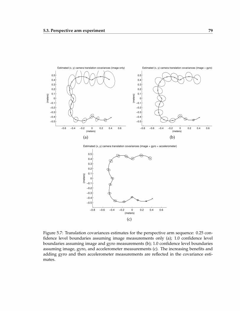
5.3. Perspective arm experiment 79
−0.6 −0.4 −0.2 0 0.2 0.4 0.6
−0.5
−0.4
−0.3
−0.2
−0.1
0
0.1
0.2
0.3
0.4
0.5
Estimated (x, y) camera translation covariances (image only)
(meters)
(met
ers)
−0.8 −0.6 −0.4 −0.2 0 0.2 0.4 0.6
−0.5
−0.4
−0.3
−0.2
−0.1
0
0.1
0.2
0.3
0.4
0.5
Estimated (x, y) camera translation covariances (image + gyro)
(meters)(m
eter
s)
(a) (b)
−0.8 −0.6 −0.4 −0.2 0 0.2 0.4 0.6
−0.5
−0.4
−0.3
−0.2
−0.1
0
0.1
0.2
0.3
0.4
0.5
Estimated (x, y) camera translation covariances (image + gyro + accelerometer)
(meters)
(met
ers)
(c)
Figure 5.7: Translation covariances estimates for the perspective arm sequence: 0.25 con-fidence level boundaries assuming image measurements only (a); 1.0 confidence levelboundaries assuming image and gyro measurements (b); 1.0 confidence level boundariesassuming image, gyro, and accelerometer measurements (c). The increasing benefits andadding gyro and then accelerometer measurements are reflected in the covariance esti-mates.
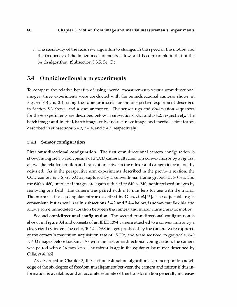
80 Chapter 5. Motion from image and inertial measurements: experiments
8. The sensitivity of the recursive algorithm to changes in the speed of the motion andthe frequency of the image measurements is low, and is comparable to that of thebatch algorithm. (Subsection 5.3.5, Set C.)
5.4 Omnidirectional arm experiments
To compare the relative benefits of using inertial measurements versus omnidirectionalimages, three experiments were conducted with the omnidirectional cameras shown inFigures 3.3 and 3.4, using the same arm used for the perspective experiment describedin Section 5.3 above, and a similar motion. The sensor rigs and observation sequencesfor these experiments are described below in subsections 5.4.1 and 5.4.2, respectively. Thebatch image-and-inertial, batch image-only, and recursive image-and-inertial estimates aredescribed in subsections 5.4.3, 5.4.4, and 5.4.5, respectively.
5.4.1 Sensor configuration
First omnidirectional configuration. The first omnidirectional camera configuration isshown in Figure 3.3 and consists of a CCD camera attached to a convex mirror by a rig thatallows the relative rotation and translation between the mirror and camera to be manuallyadjusted. As in the perspective arm experiments described in the previous section, theCCD camera is a Sony XC-55, captured by a conventional frame grabber at 30 Hz, andthe 640 × 480, interlaced images are again reduced to 640 × 240, noninterlaced images byremoving one field. The camera was paired with a 16 mm lens for use with the mirror.The mirror is the equiangular mirror described by Ollis, et al.[46]. The adjustable rig isconvenient, but as we’ll see in subsections 5.4.2 and 5.4.4 below, is somewhat flexible andallows some unmodeled vibration between the camera and mirror during erratic motion.
Second omnidirectional configuration. The second omnidirectional configuration isshown in Figure 3.4 and consists of an IEEE 1394 camera attached to a convex mirror by aclear, rigid cylinder. The color, 1042 × 768 images produced by the camera were capturedat the camera’s maximum acquisition rate of 15 Hz, and were reduced to greyscale, 640× 480 images before tracking. As with the first omnidirectional configuration, the camerawas paired with a 16 mm lens. The mirror is again the equiangular mirror described byOllis, et al.[46].
As described in Chapter 3, the motion estimation algorithms can incorporate knowl-edge of the six degree of freedom misalignment between the camera and mirror if this in-formation is available, and an accurate estimate of this transformation generally increases
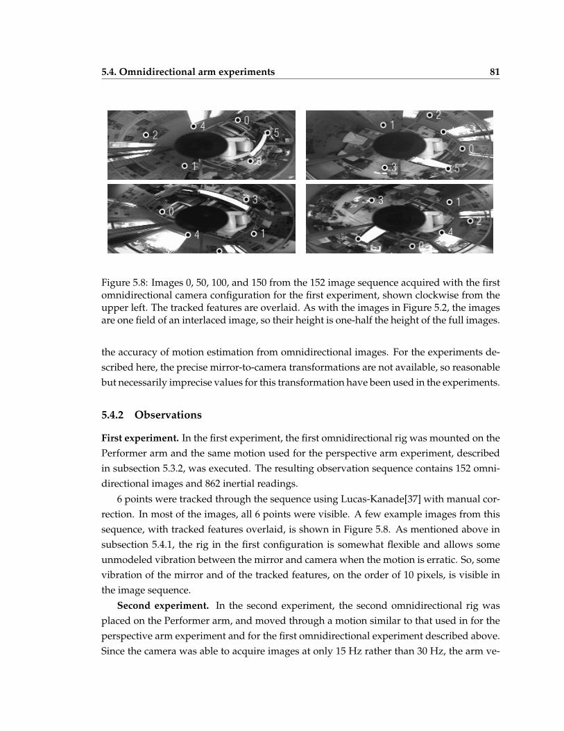
5.4. Omnidirectional arm experiments 81
Figure 5.8: Images 0, 50, 100, and 150 from the 152 image sequence acquired with the firstomnidirectional camera configuration for the first experiment, shown clockwise from theupper left. The tracked features are overlaid. As with the images in Figure 5.2, the imagesare one field of an interlaced image, so their height is one-half the height of the full images.
the accuracy of motion estimation from omnidirectional images. For the experiments de-scribed here, the precise mirror-to-camera transformations are not available, so reasonablebut necessarily imprecise values for this transformation have been used in the experiments.
5.4.2 Observations
First experiment. In the first experiment, the first omnidirectional rig was mounted on thePerformer arm and the same motion used for the perspective arm experiment, describedin subsection 5.3.2, was executed. The resulting observation sequence contains 152 omni-directional images and 862 inertial readings.
6 points were tracked through the sequence using Lucas-Kanade[37] with manual cor-rection. In most of the images, all 6 points were visible. A few example images from thissequence, with tracked features overlaid, is shown in Figure 5.8. As mentioned above insubsection 5.4.1, the rig in the first configuration is somewhat flexible and allows someunmodeled vibration between the mirror and camera when the motion is erratic. So, somevibration of the mirror and of the tracked features, on the order of 10 pixels, is visible inthe image sequence.
Second experiment. In the second experiment, the second omnidirectional rig wasplaced on the Performer arm, and moved through a motion similar to that used in for theperspective arm experiment and for the first omnidirectional experiment described above.Since the camera was able to acquire images at only 15 Hz rather than 30 Hz, the arm ve-
82 Chapter 5. Motion from image and inertial measurements: experiments
Figure 5.9: Images 0, 50, 100, and 150 from the 152 image sequence acquired with thesecond omnidirectional camera configuration for the second experiment, shown clockwisefrom the upper left. The tracked features are overlaid. In this experiment, the cameraproduces full resolution, noninterlaced images.
locity was reduced to half to produce an image sequence with the same number of imagesas the sequence used in the first experiment; inertial measurements were acquired at thesame rate as in the previous experiments. The resulting observation sequence contains 152omnidirectional images and 1853 inertial readings.
8 points were tracked through the entire sequence using Lucas-Kanade. Mistrackingwas again common and corrected by hand. Four example images from the sequence, withthe tracked features overlaid, are shown in Figure 5.9.
Third experiment. For the third experiment, the image sequence from the second ex-periment was reduced to 640 × 240 to test the effects of image resolution on the omnidi-rectional motion estimates, and the eight points tracked in the second experiment wereretracked through the entire sequence of reduced resolution images. The inertial measure-
5.4. Omnidirectional arm experiments 83
ments are the same as in the second experiment.
Comparisons with the perspective arm dataset. The motion speed and image resolu-tion in the first omnidirectional experiment, which uses the first omnidirectional configura-tion, are the same as those used to produce the unslowed perspective arm estimates (the setA batch image-and-inertial estimates in subsection 5.3.3, the batch image-only estimates insubsection 5.3.4, and the set A and B recursive image-and-inertial estimates in subsection5.3.5). So, the batch image-and-inertial, batch image-only, and recursive image-and-inertialestimates produced from this omnidirectional dataset can be compared against those de-scribed in Table 5.1, rows labeled “?”; Table 5.1, row labeled “image only”; and Tables 5.5and 5.6, respectively. One caveat is that, as we’ll see below in subsection 5.4.4, the unmod-eled vibration in the first omnidirectional experiment introduces local motion errors in theimage-only estimates. Since this unmodeled vibration is not an inherent flaw in omnidi-rectional cameras, this should be considered when comparing the image-only estimatesfrom the perspective arm experiment and the first omnidirectional arm experiment.
The motion speed and image resolution in the third omnidirectional experiment, whichuses the second omnidirectional configuration and vertically reduced images, are the sameas those used to produce the slowed perspective arm estimates with the slowdown factorf = 2 (the set B batch image-and-inertial estimates in subsection 5.3.3 and the set C re-cursive image-and-inertial estimates in subsection 5.3.5). So, the batch image-and-inertialand recursive image-and-inertial estimates from this omnidirectional experiment can becompared against those described in Table 5.2, f = 2; and Table 5.7, line 2, respectively.
5.4.3 Batch image-and-inertial estimates
For each of the three experiments a batch image-and-inertial estimate of the motion andother unknowns was generated, using an estimate from the recursive image-and-inertialmethod as the initial estimate; these recursive estimates are described below in subsection5.4.5. Based on the results in subsection 5.3.3 exploring the accuracy of estimates as afunction of the inertial error variances for the perspective sequence, inertial error variancesof 10−5 have been used for each omnidirectional experiment.
The error statistics for each of the three batch image-and-inertial estimates are givenin Table 5.8, and the x, y translation estimates from the first and second experiment areshown as the dash-dotted lines in Figure 5.10. In each experiment, the estimates suffersomewhat from the lack of a precise camera-to-mirror transformation calibration, but theresults are comparable to those in the perspective arm experiment, despite the changes inmotion speed, frame rate, and image resolution across the three experiments.
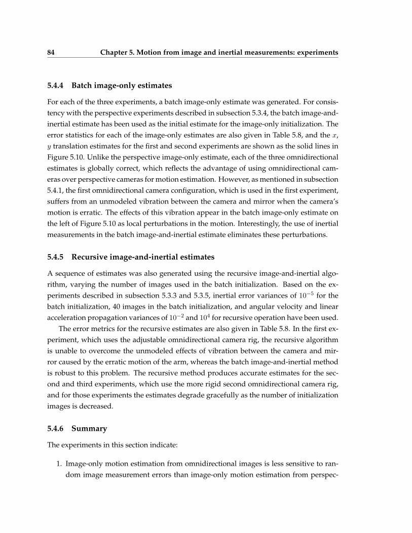
84 Chapter 5. Motion from image and inertial measurements: experiments
5.4.4 Batch image-only estimates
For each of the three experiments, a batch image-only estimate was generated. For consis-tency with the perspective experiments described in subsection 5.3.4, the batch image-and-inertial estimate has been used as the initial estimate for the image-only initialization. Theerror statistics for each of the image-only estimates are also given in Table 5.8, and the x,y translation estimates for the first and second experiments are shown as the solid lines inFigure 5.10. Unlike the perspective image-only estimate, each of the three omnidirectionalestimates is globally correct, which reflects the advantage of using omnidirectional cam-eras over perspective cameras for motion estimation. However, as mentioned in subsection5.4.1, the first omnidirectional camera configuration, which is used in the first experiment,suffers from an unmodeled vibration between the camera and mirror when the camera’smotion is erratic. The effects of this vibration appear in the batch image-only estimate onthe left of Figure 5.10 as local perturbations in the motion. Interestingly, the use of inertialmeasurements in the batch image-and-inertial estimate eliminates these perturbations.
5.4.5 Recursive image-and-inertial estimates
A sequence of estimates was also generated using the recursive image-and-inertial algo-rithm, varying the number of images used in the batch initialization. Based on the ex-periments described in subsection 5.3.3 and 5.3.5, inertial error variances of 10−5 for thebatch initialization, 40 images in the batch initialization, and angular velocity and linearacceleration propagation variances of 10−2 and 104 for recursive operation have been used.
The error metrics for the recursive estimates are also given in Table 5.8. In the first ex-periment, which uses the adjustable omnidirectional camera rig, the recursive algorithmis unable to overcome the unmodeled effects of vibration between the camera and mir-ror caused by the erratic motion of the arm, whereas the batch image-and-inertial methodis robust to this problem. The recursive method produces accurate estimates for the sec-ond and third experiments, which use the more rigid second omnidirectional camera rig,and for those experiments the estimates degrade gracefully as the number of initializationimages is decreased.
5.4.6 Summary
The experiments in this section indicate:
1. Image-only motion estimation from omnidirectional images is less sensitive to ran-dom image measurement errors than image-only motion estimation from perspec-
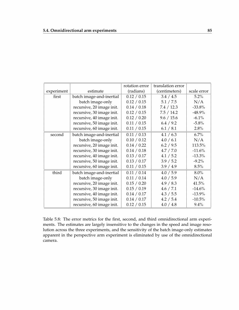
5.4. Omnidirectional arm experiments 85
rotation error translation errorexperiment estimate (radians) (centimeters) scale error
first batch image-and-inertial 0.12 / 0.15 3.4 / 4.5 5.2%batch image-only 0.12 / 0.15 5.1 / 7.5 N/A
recursive, 20 image init. 0.14 / 0.18 7.4 / 12.3 -33.8%recursive, 30 image init. 0.12 / 0.15 7.5 / 14.2 -48.9%recursive, 40 image init. 0.12 / 0.20 9.6 / 15.6 -6.1%recursive, 50 image init. 0.11 / 0.15 6.4 / 9.2 -5.8%recursive, 60 image init. 0.11 / 0.15 6.1 / 8.1 2.8%
second batch image-and-inertial 0.11 / 0.13 4.1 / 6.3 6.7%batch image-only 0.10 / 0.12 4.0 / 6.1 N/A
recursive, 20 image init. 0.14 / 0.22 6.2 / 9.5 113.5%recursive, 30 image init. 0.14 / 0.18 4.7 / 7.0 -11.6%recursive, 40 image init. 0.13 / 0.17 4.1 / 5.2 -13.3%recursive, 50 image init. 0.13 / 0.17 3.9 / 5.2 -9.2%recursive, 60 image init. 0.11 / 0.15 3.9 / 4.9 8.5%
third batch image-and-inertial 0.11 / 0.14 4.0 / 5.9 8.0%batch image-only 0.11 / 0.14 4.0 / 5.9 N/A
recursive, 20 image init. 0.15 / 0.20 4.9 / 8.3 41.5%recursive, 30 image init. 0.15 / 0.19 4.6 / 7.1 -14.6%recursive, 40 image init. 0.14 / 0.17 4.3 / 5.5 -13.9%recursive, 50 image init. 0.14 / 0.17 4.2 / 5.4 -10.5%recursive, 60 image init. 0.12 / 0.15 4.0 / 4.8 9.4%
Table 5.8: The error metrics for the first, second, and third omnidirectional arm experi-ments. The estimates are largely insensitive to the changes in the speed and image reso-lution across the three experiments, and the sensitivity of the batch image-only estimatesapparent in the perspective arm experiment is eliminated by use of the omnidirectionalcamera.
86 Chapter 5. Motion from image and inertial measurements: experiments
−0.8 −0.6 −0.4 −0.2 0 0.2 0.4 0.6
−0.5
−0.4
−0.3
−0.2
−0.1
0
0.1
0.2
0.3
0.4
0.5
Estimated (x, y) camera translations
(meters)
(met
ers)
−0.8 −0.6 −0.4 −0.2 0 0.2 0.4 0.6
−0.5
−0.4
−0.3
−0.2
−0.1
0
0.1
0.2
0.3
0.4
0.5
Estimated (x, y) camera translations
(meters)
(met
ers)
(a) (b)
Figure 5.10: The x, y translation estimates generated by the batch image-and-inertial andbatch image-only algorithms for the first and second omnidirectional arm experiments.Left: The estimates generated by the batch image-and-inertial algorithm and by the batchimage-only algorithm for the first omnidirectional experiment are shown as the dash-dotted and solid lines, respectively. Right: The estimates generated by the batch image-and-inertial algorithm and by the batch image-only algorithm for the second omnidirec-tional experiment are shown as the dash-dotted and solid lines, respectively. On both theleft and right, the x, y locations of the seven known ground truth points are shown assquares.
5.5. Perspective crane experiment 87
tive images, so the advantage of incorporating inertial measurements is less for om-nidirectional images than for perspective images. (Subsections 5.4.3 and 5.4.4.)
2. The incorporation of inertial measurements in the batch image-and-inertial algo-rithm provides some robustness to moderate, nonrandom image measurement er-rors, in this case unmodeled vibration between the mirror and camera in the firstexperiment. (Subsections 5.4.3 and 5.4.4.)
3. The recursive image-and-inertial algorithm produces poor estimates in the presenceof nonrandom image measurement errors in the first experiment, despite the incor-poration of inertial measurements. (Subsection 5.4.5.)
5.5 Perspective crane experiment
5.5.1 Camera configuration
The camera configuration for the perspective crane experiment is the same as that for per-spective arm experiment, except that to gain a wider field of view, a 3.5 mm lens was usedin place of the 6 mm lens.
5.5.2 Observations
The rig was mounted on the platform of a specially constructed crane that translates theplatform within a 10 m× 10 m× 5 m area. For the experiment, the crane was programmedto move between eleven prespecified control points. These points take the platform fromthe center of the work area to one corner of a 6 meter wide square aligned with the cranecoordinate system (x, y), around the square, and then back to the center of the work area.In z, the platform translates 1 m between adjacent control points, alternating between highand low positions.
The observation sequence taken during this circuit consists of 1430 images and 51553inertial readings spanning 4 minutes and 46 seconds; eight example images from the se-quence are shown in Figure 5.11. 100 points were extracted in the first image of the se-quence, and tracked through the sequence using Lucas-Kanade. In subsequent images inwhich the number of tracked points fell below 80 due to features leaving the field of view,becoming occluded, or changing appearance, reextraction was used to bring the number oftracked points back to 100. Many mistracked points were identified by applying RANSACin conjunction with batch, image-only shape and motion estimation to each subsequence
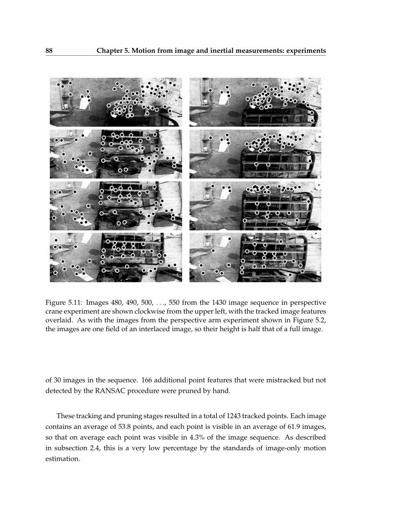
88 Chapter 5. Motion from image and inertial measurements: experiments
Figure 5.11: Images 480, 490, 500, . . ., 550 from the 1430 image sequence in perspectivecrane experiment are shown clockwise from the upper left, with the tracked image featuresoverlaid. As with the images from the perspective arm experiment shown in Figure 5.2,the images are one field of an interlaced image, so their height is half that of a full image.
of 30 images in the sequence. 166 additional point features that were mistracked but notdetected by the RANSAC procedure were pruned by hand.
These tracking and pruning stages resulted in a total of 1243 tracked points. Each imagecontains an average of 53.8 points, and each point is visible in an average of 61.9 images,so that on average each point was visible in 4.3% of the image sequence. As describedin subsection 2.4, this is a very low percentage by the standards of image-only motionestimation.
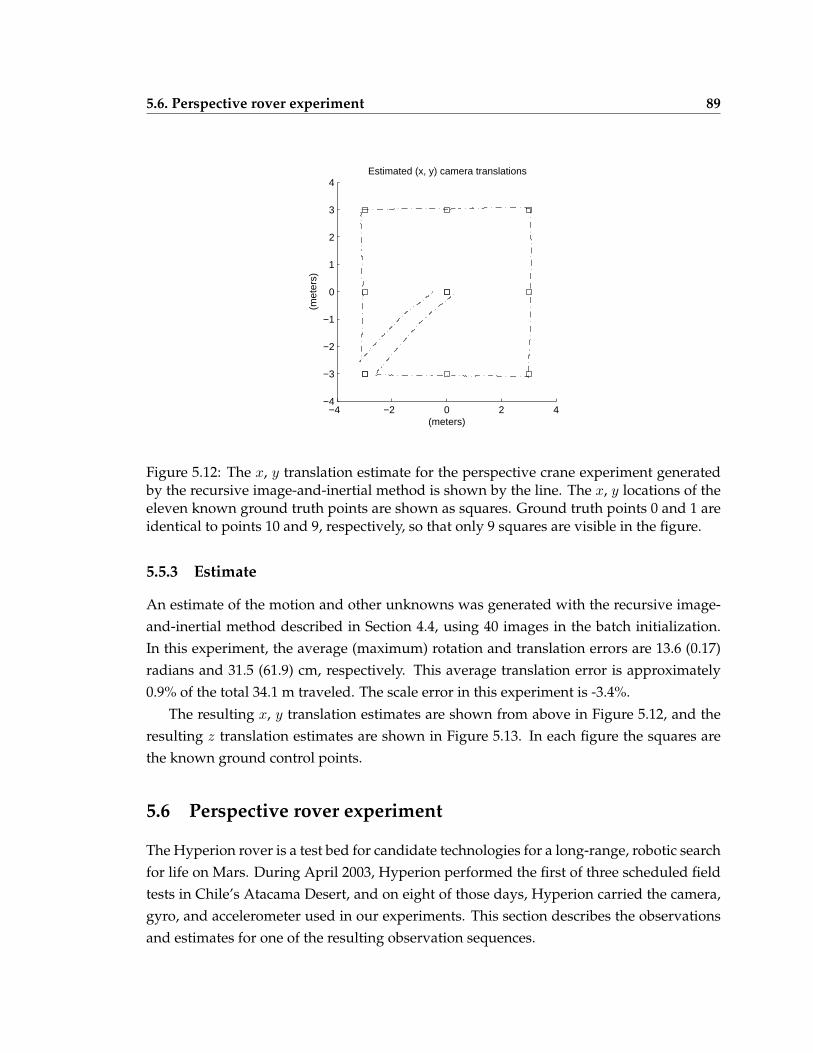
5.6. Perspective rover experiment 89
−4 −2 0 2 4−4
−3
−2
−1
0
1
2
3
4Estimated (x, y) camera translations
(meters)
(met
ers)
Figure 5.12: The x, y translation estimate for the perspective crane experiment generatedby the recursive image-and-inertial method is shown by the line. The x, y locations of theeleven known ground truth points are shown as squares. Ground truth points 0 and 1 areidentical to points 10 and 9, respectively, so that only 9 squares are visible in the figure.
5.5.3 Estimate
An estimate of the motion and other unknowns was generated with the recursive image-and-inertial method described in Section 4.4, using 40 images in the batch initialization.In this experiment, the average (maximum) rotation and translation errors are 13.6 (0.17)radians and 31.5 (61.9) cm, respectively. This average translation error is approximately0.9% of the total 34.1 m traveled. The scale error in this experiment is -3.4%.
The resulting x, y translation estimates are shown from above in Figure 5.12, and theresulting z translation estimates are shown in Figure 5.13. In each figure the squares arethe known ground control points.
5.6 Perspective rover experiment
The Hyperion rover is a test bed for candidate technologies for a long-range, robotic searchfor life on Mars. During April 2003, Hyperion performed the first of three scheduled fieldtests in Chile’s Atacama Desert, and on eight of those days, Hyperion carried the camera,gyro, and accelerometer used in our experiments. This section describes the observationsand estimates for one of the resulting observation sequences.
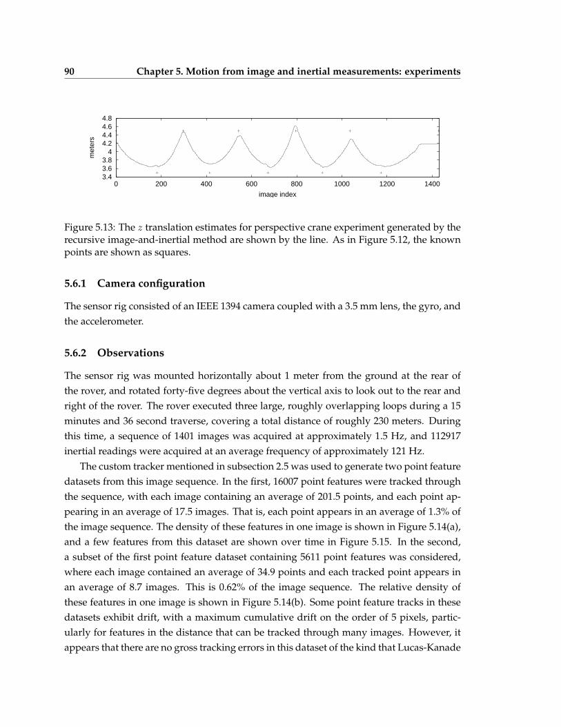
90 Chapter 5. Motion from image and inertial measurements: experiments
3.43.63.8
44.24.44.64.8
0 200 400 600 800 1000 1200 1400
met
ers
image index
Figure 5.13: The z translation estimates for perspective crane experiment generated by therecursive image-and-inertial method are shown by the line. As in Figure 5.12, the knownpoints are shown as squares.
5.6.1 Camera configuration
The sensor rig consisted of an IEEE 1394 camera coupled with a 3.5 mm lens, the gyro, andthe accelerometer.
5.6.2 Observations
The sensor rig was mounted horizontally about 1 meter from the ground at the rear ofthe rover, and rotated forty-five degrees about the vertical axis to look out to the rear andright of the rover. The rover executed three large, roughly overlapping loops during a 15minutes and 36 second traverse, covering a total distance of roughly 230 meters. Duringthis time, a sequence of 1401 images was acquired at approximately 1.5 Hz, and 112917inertial readings were acquired at an average frequency of approximately 121 Hz.
The custom tracker mentioned in subsection 2.5 was used to generate two point featuredatasets from this image sequence. In the first, 16007 point features were tracked throughthe sequence, with each image containing an average of 201.5 points, and each point ap-pearing in an average of 17.5 images. That is, each point appears in an average of 1.3% ofthe image sequence. The density of these features in one image is shown in Figure 5.14(a),and a few features from this dataset are shown over time in Figure 5.15. In the second,a subset of the first point feature dataset containing 5611 point features was considered,where each image contained an average of 34.9 points and each tracked point appears inan average of 8.7 images. This is 0.62% of the image sequence. The relative density ofthese features in one image is shown in Figure 5.14(b). Some point feature tracks in thesedatasets exhibit drift, with a maximum cumulative drift on the order of 5 pixels, partic-ularly for features in the distance that can be tracked through many images. However, itappears that there are no gross tracking errors in this dataset of the kind that Lucas-Kanade
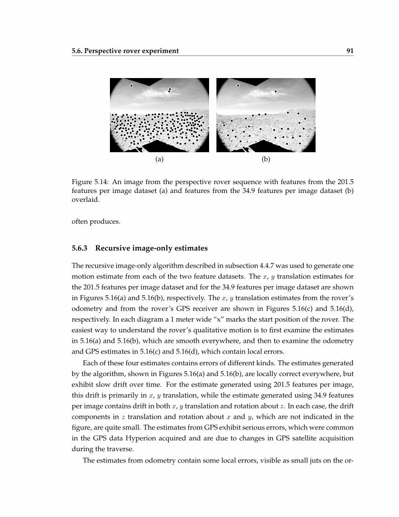
5.6. Perspective rover experiment 91
(a) (b)
Figure 5.14: An image from the perspective rover sequence with features from the 201.5features per image dataset (a) and features from the 34.9 features per image dataset (b)overlaid.
often produces.
5.6.3 Recursive image-only estimates
The recursive image-only algorithm described in subsection 4.4.7 was used to generate onemotion estimate from each of the two feature datasets. The x, y translation estimates forthe 201.5 features per image dataset and for the 34.9 features per image dataset are shownin Figures 5.16(a) and 5.16(b), respectively. The x, y translation estimates from the rover’sodometry and from the rover’s GPS receiver are shown in Figures 5.16(c) and 5.16(d),respectively. In each diagram a 1 meter wide “x” marks the start position of the rover. Theeasiest way to understand the rover’s qualitative motion is to first examine the estimatesin 5.16(a) and 5.16(b), which are smooth everywhere, and then to examine the odometryand GPS estimates in 5.16(c) and 5.16(d), which contain local errors.
Each of these four estimates contains errors of different kinds. The estimates generatedby the algorithm, shown in Figures 5.16(a) and 5.16(b), are locally correct everywhere, butexhibit slow drift over time. For the estimate generated using 201.5 features per image,this drift is primarily in x, y translation, while the estimate generated using 34.9 featuresper image contains drift in both x, y translation and rotation about z. In each case, the driftcomponents in z translation and rotation about x and y, which are not indicated in thefigure, are quite small. The estimates from GPS exhibit serious errors, which were commonin the GPS data Hyperion acquired and are due to changes in GPS satellite acquisitionduring the traverse.
The estimates from odometry contain some local errors, visible as small juts on the or-
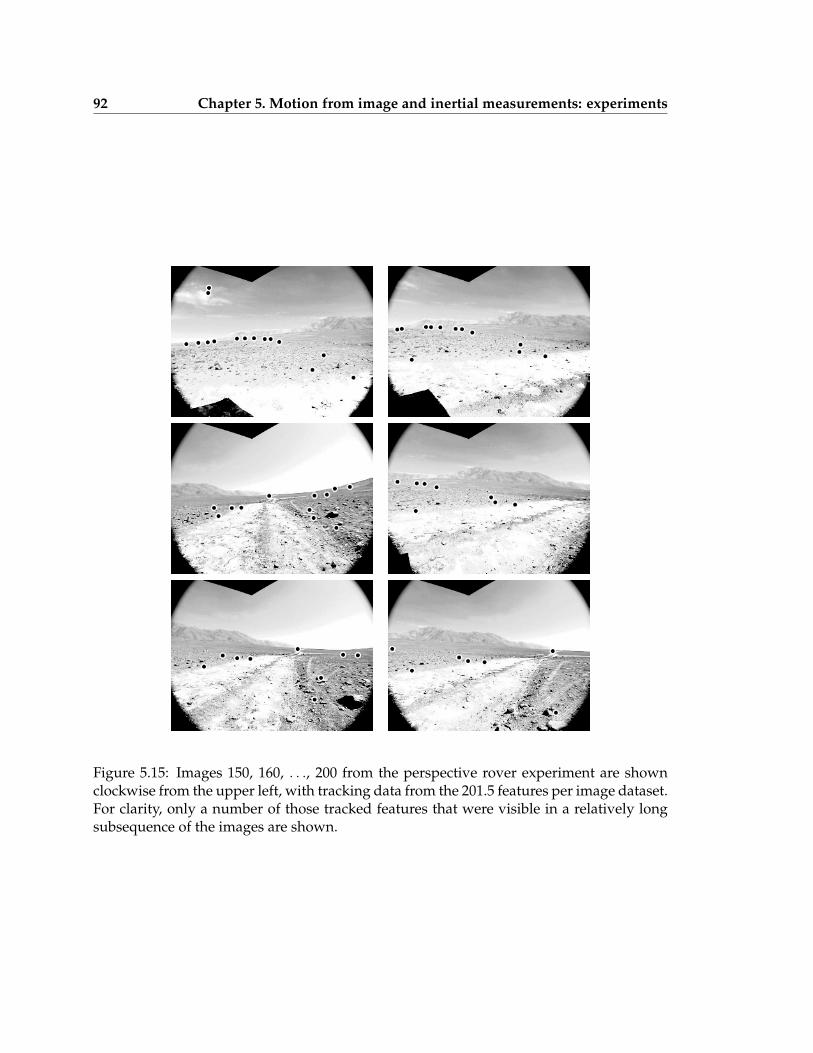
92 Chapter 5. Motion from image and inertial measurements: experiments
Figure 5.15: Images 150, 160, . . ., 200 from the perspective rover experiment are shownclockwise from the upper left, with tracking data from the 201.5 features per image dataset.For clarity, only a number of those tracked features that were visible in a relatively longsubsequence of the images are shown.
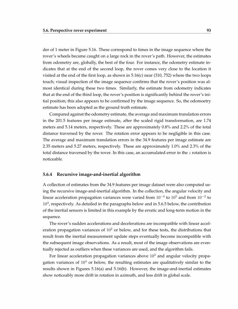
5.6. Perspective rover experiment 93
der of 1 meter in Figure 5.16. These correspond to times in the image sequence where therover’s wheels became caught on a large rock in the rover’s path. However, the estimatesfrom odometry are, globally, the best of the four. For instance, the odometry estimate in-dicates that at the end of the second loop, the rover comes very close to the location itvisited at the end of the first loop, as shown in 5.16(c) near (310, 752) where the two loopstouch; visual inspection of the image sequence confirms that the rover’s position was al-most identical during these two times. Similarly, the estimate from odometry indicatesthat at the end of the third loop, the rover’s position is significantly behind the rover’s ini-tial position; this also appears to be confirmed by the image sequence. So, the odomoetryestimate has been adopted as the ground truth estimate.
Compared against the odometry estimate, the average and maximum translation errorsin the 201.5 features per image estimate, after the scaled rigid transformation, are 1.74meters and 5.14 meters, respectively. These are approximately 0.8% and 2.2% of the totaldistance traversed by the rover. The rotation error appears to be negligible in this case.The average and maximum translation errors in the 34.9 features per image estimate are2.35 meters and 5.27 meters, respectively. These are approximately 1.0% and 2.3% of thetotal distance traversed by the rover. In this case, an accumulated error in the z rotation isnoticeable.
5.6.4 Recursive image-and-inertial algorithm
A collection of estimates from the 34.9 features per image dataset were also computed us-ing the recursive image-and-inertial algorithm. In the collection, the angular velocity andlinear acceleration propagation variances were varied from 10−4 to 105 and from 10−2 to104, respectively. As detailed in the paragraphs below and in 5.6.5 below, the contributionof the inertial sensors is limited in this example by the erratic and long-term motion in thesequence.
The rover’s sudden accelerations and decelerations are incompatible with linear accel-eration propagation variances of 102 or below, and for these tests, the distributions thatresult from the inertial measurement update steps eventually become incompatible withthe subsequent image observations. As a result, most of the image observations are even-tually rejected as outliers when these variances are used, and the algorithm fails.
For linear acceleration propagation variances above 102 and angular velocity propa-gation variances of 104 or below, the resulting estimates are qualitatively similar to theresults shown in Figures 5.16(a) and 5.16(b). However, the image-and-inertial estimatesshow noticeably more drift in rotation in azimuth, and less drift in global scale.
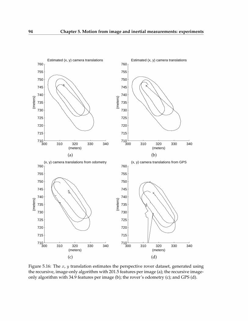
94 Chapter 5. Motion from image and inertial measurements: experiments
300 310 320 330 340710
715
720
725
730
735
740
745
750
755
760Estimated (x, y) camera translations
(meters)
(met
ers)
300 310 320 330 340710
715
720
725
730
735
740
745
750
755
760Estimated (x, y) camera translations
(meters)
(met
ers)
(a) (b)
300 310 320 330 340710
715
720
725
730
735
740
745
750
755
760(x, y) camera translations from odometry
(meters)
(met
ers)
300 310 320 330 340710
715
720
725
730
735
740
745
750
755
760(x, y) camera translations from GPS
(meters)
(met
ers)
(c) (d)
Figure 5.16: The x, y translation estimates the perspective rover dataset, generated usingthe recursive, image-only algorithm with 201.5 features per image (a); the recursive image-only algorithm with 34.9 features per image (b); the rover’s odometry (c); and GPS (d).
5.6. Perspective rover experiment 95
As described in subsection 4.4.8, weakening the assumption of continuity in the an-gular velocity and linear acceleration necessarily weakens the contribution of the inertialmeasurements in the recursive image-and-inertial algorithm. This is reflected in this exper-iment: for the most generous propagation variances, i.e., linear acceleration propagationvariances above 102 an angular velocity variance of 105, respectively, the effect of the in-ertial measurements becomes negligible, and the estimates are almost identical to the 34.9features per image, recursive image-only estimate shown in Figure 5.16(b).
5.6.5 Discussion
In this experiment, the image-only motion estimates benefit from dense, high-quality fea-ture tracking data, and are locally correct everywhere as a result. However, due to thesmall number of images in which each point feature is visible, the motion is not beingestimated with respect to any one external point, and so necessarily drifts with time.
Long-term drift in the image-only estimates to be a type of ambiguity, in the sense thatthe true, globally correct motion and a large space of drifting estimates will all producesmall reprojection errors. In fact, given that the image observations and the camera cali-bration both contain small errors, the estimate that best minimizes the reprojection errorwill almost never be a globally correct estimate, but will contain some drift. This is in con-trast to cases such as that described in Section 5.3, where only sparse, noisy tracking datais available, and where even the local motion cannot be uniquely identified from imagemeasurements alone.
Can the incorporation of measurements from inexpensive inertial sensors remove thisambiguity in the long-term motion, if the image-only estimates are locally correct every-where? Since the sensors’ absolute orientation with respect to gravity can be reliably foundby separating the effects of gravity and the other unknowns in the accelerometer read-ings, inexpensive inertial sensors can eliminate long-term drift in the estimated rotationabout the two axes perpendicular to the gravity direction. (In the image-only estimatesdescribed in subsection 5.6.3, the drift in these two components of the rotation was notsignificant when compared to the drift in the rotation about the gravity direction and inthe x, y translation, so orientation information from the accelerometer was not needed.)However, inexpensive inertial sensors are unlikely to resolve long-term drift in the trans-lation or in the rotation about the gravity direction, because the rate of drift in the inertialsensor estimates is likely to be much faster than that of the image-only estimates.
On the other hand, can the incorporation of measurements from inexpensive inertialsensors improve long-term motion estimates if the image-only estimates are locally am-
96 Chapter 5. Motion from image and inertial measurements: experiments
biguous at some points? Of course, in this case the inertial sensors can improve the long-term motion by resolving these ambiguities, which may turn a qualitatively wrong esti-mate into an accurate estimate. However, estimates will drift less slowly if the image-onlyestimates can be made locally correct (e.g., by obtaining dense feature tracking data), thanif the image-only estimates are locally ambiguous (e.g., generated using sparse image data)and inertial measurements are incorporated to resolve the local ambiguities.
Chapter 6
Robust feature tracking for motionestimation
6.1 Overview
As the experiments in Chapter 5 show, motion estimation from sparse image features canbe sensitive to even small errors in the input projections, even when the motion is esti-mated using an optimal algorithm. As discussed in subsection 5.3.4, these errors are dueto both:
• feature tracking errors
• errors that result from normalizing image measurements with uncertain camera in-trinsics
Feature tracking errors might be slowing accumulating errors that result from tracking apoint over a long image sequence, or more sudden errors between adjacent images that re-sult from occlusions, lighting changes, specularities, or other difficulties common in imagetracking. As a result, the motion estimates produced from the projections can:
• contain local errors
• be locally correct everywhere but contain long-term drift
Local errors are immediate problems because significant errors between adjacent cam-era position estimates produce large errors in the estimated positions of points visible fromthose camera positions; in turn, these produce unrecoverable gross errors in the next fewcamera position estimates. But, long-term drift is a more fundamental problem, since no
97
98 Chapter 6. Robust feature tracking for motion estimation
level of accuracy in the tracking and camera intrinsics can eliminate drift completely. So,image-based motion estimation places high demands on both image feature tracking andcamera calibration.
This chapter describes a new tracking algorithm designed to reduce both local errorsand long-term drift in image-based motion estimation. The algorithm exploits severalobservations:
• SIFT keypoints[36], described in Section 2.6, provide a convenient way to estimatethe epipolar geometry between images with no problematic assumptions on the cam-era motion.
• Features do not move arbitrarily between images, as assumed when tracking featuresindividually in two dimensions, but are constrained by the rigid scene assumption.So, each feature should be tracked in one dimension along its epipolar line in its newimage.
• Motion estimation benefits from a wide field of view, but the field of view is effec-tively reduced if features are not tracked throughout the entire image. So, featuresshould be extracted to achieve a wide effective field of view.
• Poorly textured features can often be correctly tracked when constrained to one di-mension. So, texture should be a secondary criterion for extraction rather than theprimary criterion.
• For image-based motion estimation, features that become clustered during tracking(e.g., by moving towards a common vanishing point) are redundant and should bepruned. Since the oldest feature in an image neighborhood is likely to provide themost information for camera motion estimation, younger features should be prunedaway before older features.
• A feature whose appearance did not change between images may be incorrectlytracked (e.g., a feature that jumps between similar areas on a repetitive texture) and afeature whose appearance changed drastically between two images may be trackedprecisely, especially when constrained to the epipolar line. So, changes in image ap-pearance should be rejected as a criterion for detecting mistracking.
The resulting algorithm can track with high robustness and accuracy in many sequencesfor which the previous go-to tracker, Lucas-Kanade, fails. In addition, the resulting distri-bution of features is more appropriate for motion estimation. As a result of these improve-
6.2. Lucas-Kanade 99
ments in feature tracking, local errors in six degree of freedom motion estimates are oftencompletely eliminated.
The remaining sections of this chapter are organized as follows. Lucas-Kanade, whichhas long been the go-to tracker for shape-from-motion, and the problems in using it forreal sequences are reviewed in Section 6.2 and 6.3, respectively. Because the new trackerestimates and uses the epipolar geometry between adjacent images in the sequence, Sec-tion 6.4 reviews the epipolar geometry between images and the fundamental matrix thatdescribes it. The design of the new tracker is described in detail in Section 6.5, and experi-mental results are given in Sections 6.6, 6.7, and 6.8 below. The new algorithm’s limitationsand possible further improvements are described in 6.9.
As mentioned at the beginning of this section and in Section 2.9, motion estimationaccuracy is limited by camera intrinsics errors as well as tracking errors. This work hasnot investigated improved models for conventional cameras, but better conventional cam-era models are a promising approach for improving both motion estimation and featuretracking.
6.2 Lucas-Kanade
Lucas-Kanade[37] has long been the preferred sparse feature tracker for shape-from-motion.In brief, Lucas-Kanade finds a template’s match location in a new image by using second-order iterative optimization to minimize the sum-of-squared-differences (SSD) betweenthe template and image intensities. Typically, the template’s location is taken to be the (x,y) translation, but the SSD is sometimes minimized with respect to an affine or other moregeneral transformation of the template.
To track features in an image sequence taken from a moving camera, Lucas-Kanade isnormally used with three heuristics:
• Features that maximize the conditioning of the system solved by Lucas-Kanade oneach iteration are extracted for tracking. This approach results in features near highimage texture, and rejects features in textureless areas or areas where the texture isone-dimensional.
• A feature is marked as mistracked and discarded if the Lucas-Kanade iterations failto converge, or if the SSD error at the minimum is larger than a predefined thresh-old. In the second case, the feature is marked as mistracked because it has changedappearance.
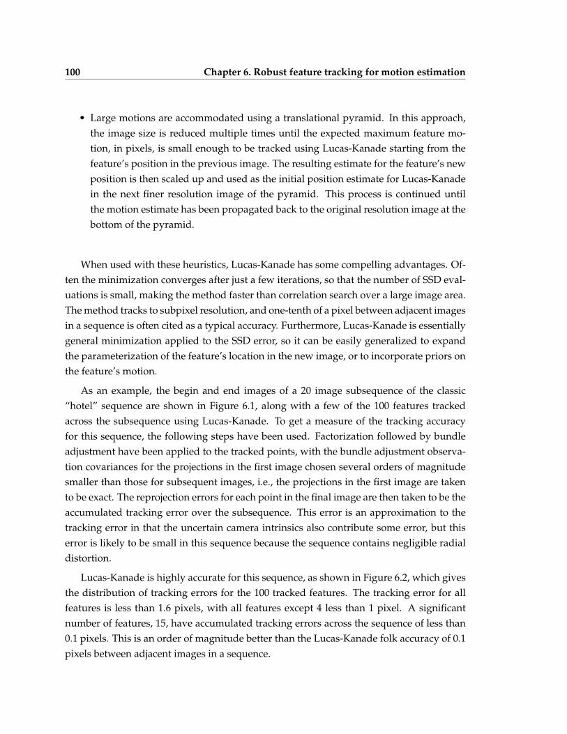
100 Chapter 6. Robust feature tracking for motion estimation
• Large motions are accommodated using a translational pyramid. In this approach,the image size is reduced multiple times until the expected maximum feature mo-tion, in pixels, is small enough to be tracked using Lucas-Kanade starting from thefeature’s position in the previous image. The resulting estimate for the feature’s newposition is then scaled up and used as the initial position estimate for Lucas-Kanadein the next finer resolution image of the pyramid. This process is continued untilthe motion estimate has been propagated back to the original resolution image at thebottom of the pyramid.
When used with these heuristics, Lucas-Kanade has some compelling advantages. Of-ten the minimization converges after just a few iterations, so that the number of SSD eval-uations is small, making the method faster than correlation search over a large image area.The method tracks to subpixel resolution, and one-tenth of a pixel between adjacent imagesin a sequence is often cited as a typical accuracy. Furthermore, Lucas-Kanade is essentiallygeneral minimization applied to the SSD error, so it can be easily generalized to expandthe parameterization of the feature’s location in the new image, or to incorporate priors onthe feature’s motion.
As an example, the begin and end images of a 20 image subsequence of the classic“hotel” sequence are shown in Figure 6.1, along with a few of the 100 features trackedacross the subsequence using Lucas-Kanade. To get a measure of the tracking accuracyfor this sequence, the following steps have been used. Factorization followed by bundleadjustment have been applied to the tracked points, with the bundle adjustment observa-tion covariances for the projections in the first image chosen several orders of magnitudesmaller than those for subsequent images, i.e., the projections in the first image are takento be exact. The reprojection errors for each point in the final image are then taken to be theaccumulated tracking error over the subsequence. This error is an approximation to thetracking error in that the uncertain camera intrinsics also contribute some error, but thiserror is likely to be small in this sequence because the sequence contains negligible radialdistortion.
Lucas-Kanade is highly accurate for this sequence, as shown in Figure 6.2, which givesthe distribution of tracking errors for the 100 tracked features. The tracking error for allfeatures is less than 1.6 pixels, with all features except 4 less than 1 pixel. A significantnumber of features, 15, have accumulated tracking errors across the sequence of less than0.1 pixels. This is an order of magnitude better than the Lucas-Kanade folk accuracy of 0.1pixels between adjacent images in a sequence.
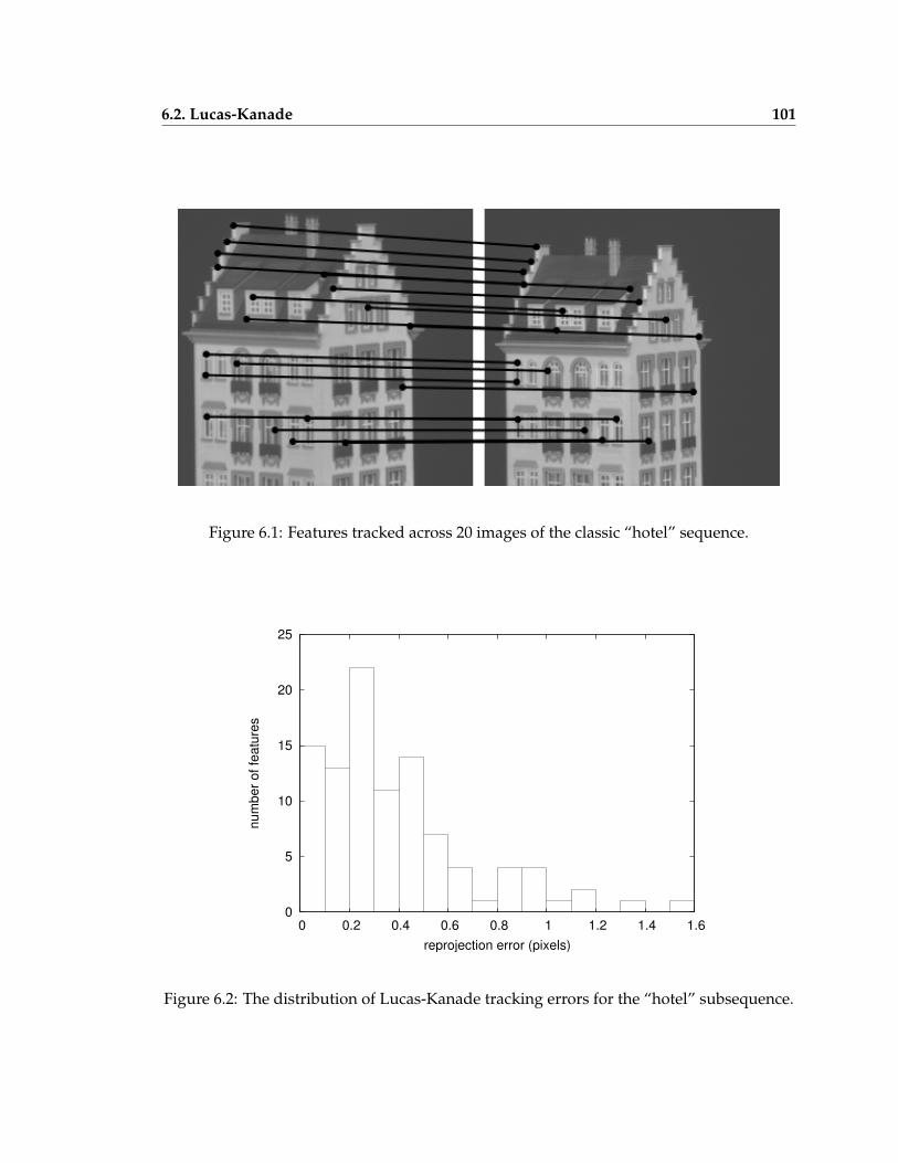
6.2. Lucas-Kanade 101
Figure 6.1: Features tracked across 20 images of the classic “hotel” sequence.
0
5
10
15
20
25
0 0.2 0.4 0.6 0.8 1 1.2 1.4 1.6
num
ber o
f fea
ture
s
reprojection error (pixels)
Figure 6.2: The distribution of Lucas-Kanade tracking errors for the “hotel” subsequence.
102 Chapter 6. Robust feature tracking for motion estimation
6.3 Lucas-Kanade and real sequences
The hotel sequence described in the previous section is benign in many ways. The features’motion between images is nearly uniform in (x, y), and therefore well modeled by Lucas-Kanade’s translational pyramid, but also small enough that the pyramid is not necessary.While the image texture is repetitive, the frequency of the repetition is low relative to thefeatures’ small motion. In addition, the features do not undergo any deformation, occlu-sion, or change in overall intensity. So, drift is minimal and Lucas-Kanade’s image-basedheuristic for detecting mistracked points works well for this sequence.
For many sequences taken from a moving camera, however, Lucas-Kanade producestracking that is unusable for motion estimation. Lucas-Kanade’s poor performance resultsfrom:
1. Unconstrained tracking. The locations of features tracked without constraints are un-duly sensitive to changes in appearance, occlusion, and low texture.
2. A poor heuristic for handling large motions. Many overall image motions are not wellmodeled by the translational pyramid. For instance, camera rotations about andcamera translations along the optical axis produce image motions that average tozero (x, y) translational motion over the image, but are actually zero at almost nospecific locations in the image. Furthermore, while the translational pyramid allowsthe tracking of some motions that are too large to be tracked with bare Lucas-Kanade,the translational pyramid sets an a priori limit on the size of motions that can betracked.
3. A poor heuristic for feature extraction. As mentioned in Section 6.1, exploiting the cam-era’s full field of view for motion estimation requires that features be extracted andtracked correctly throughout the entire image, even if some areas of the image haveonly poor texture.
4. A poor heuristic for discarding features. As mentioned in Section 6.1, changes in featureappearance, or lack thereof, are poor indications of mistracking.
Some image sequences that are problematic for Lucas-Kanade have already been shownin Chapter 5. The image sequence from the perspective arm sequence, shown in Figure 5.2,is one example. In this sequence, the large rotation about the optical axis produces largemotions in the periphery of the image that are not captured by Lucas-Kanade’s translationpyramid. The unmodeled motion is especially damaging for features on the light gratesand on the air vent, which are repetitive textures, and as a result, features jump between
6.4. Background: epipolar geometry and the fundamental matrix 103
locations on the grates and air vent. However, tracking is also poor on the styrofoam ceil-ing tiles, which have poor texture, and on the metal slats that support them, which areone-dimensional textures.
The perspective crane image sequence shown in Figure 5.11 is a second example. In thissequence, Lucas-Kanade’s translational pyramid model is appropriate. However, trackingin this sequence suffers in this sequence from repetitive texture, and gradual occlusion offeatures, and specularities.
A third example is the perspective rover image sequence shown in Figures 5.14 and5.15. In this example the translational pyramid again fails, since for much of the sequenceall of the terrain points move towards a single vanishing point on the horizon. This motionalso produces clumps of points in a single area of the image near the horizon. Lucas-Kanade’s heuristics for eliminating and extracting points also fails, producing a redundantset of points and leaving the rest of the image unpopulated.
6.4 Background: epipolar geometry and the fundamental matrix
As described in Section 6.5 below, the new tracker estimates the epipolar geometry be-tween adjacent images in the sequence and uses it to constrain the tracking between ad-jacent images. In this subsection we briefly review the epipolar geometry between twoimages and the fundamental matrix that describes it.
The epipolar geometry between two images is illustrated in Figure 6.3. Suppose thata point X is visible in the first image and that the camera’s motion between the times ofthe first and second images are known, but that the depth of X is unknown. Then anepipolar line l′ in the second image that must contain the projection x′ of X can be foundby backprojecting a ray from the first camera center c through the projection x of X in thefirst image, and then reprojecting the ray into the second image.
Since all of the rays backprojected from the first image originate from the camera centerat the time of the first image, and the epipolar lines are reprojections of these rays, all ofthe epipolar lines in the second image must intersect at the projection of the first image’scamera center in the second image. This point is called the epipole and is marked as e′ inFigure 6.3.
The essential matrix E relates corresponding normalized projections x = [x0 x1] andx′ = [x′0 x′1] in the two images through the equation:
[x0 x1 1]E[x′0 x′1 1]T = 0 (6.1)
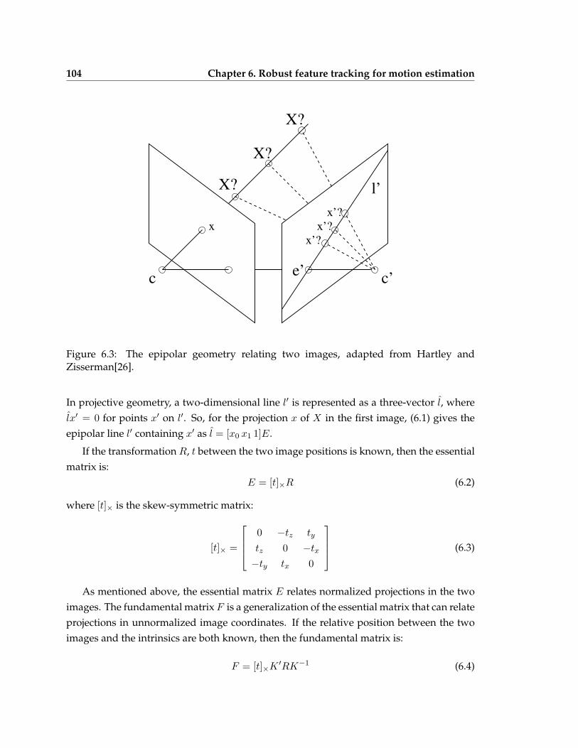
104 Chapter 6. Robust feature tracking for motion estimation
l’
c c’
xx’?
x’?x’?
X?
X?
X?
e’
Figure 6.3: The epipolar geometry relating two images, adapted from Hartley andZisserman[26].
In projective geometry, a two-dimensional line l′ is represented as a three-vector l, wherelx′ = 0 for points x′ on l′. So, for the projection x of X in the first image, (6.1) gives theepipolar line l′ containing x′ as l = [x0 x1 1]E.
If the transformation R, t between the two image positions is known, then the essentialmatrix is:
E = [t]×R (6.2)
where [t]× is the skew-symmetric matrix:
[t]× =
0 −tz ty
tz 0 −tx
−ty tx 0
(6.3)
As mentioned above, the essential matrix E relates normalized projections in the twoimages. The fundamental matrix F is a generalization of the essential matrix that can relateprojections in unnormalized image coordinates. If the relative position between the twoimages and the intrinsics are both known, then the fundamental matrix is:
F = [t]×K ′RK−1 (6.4)
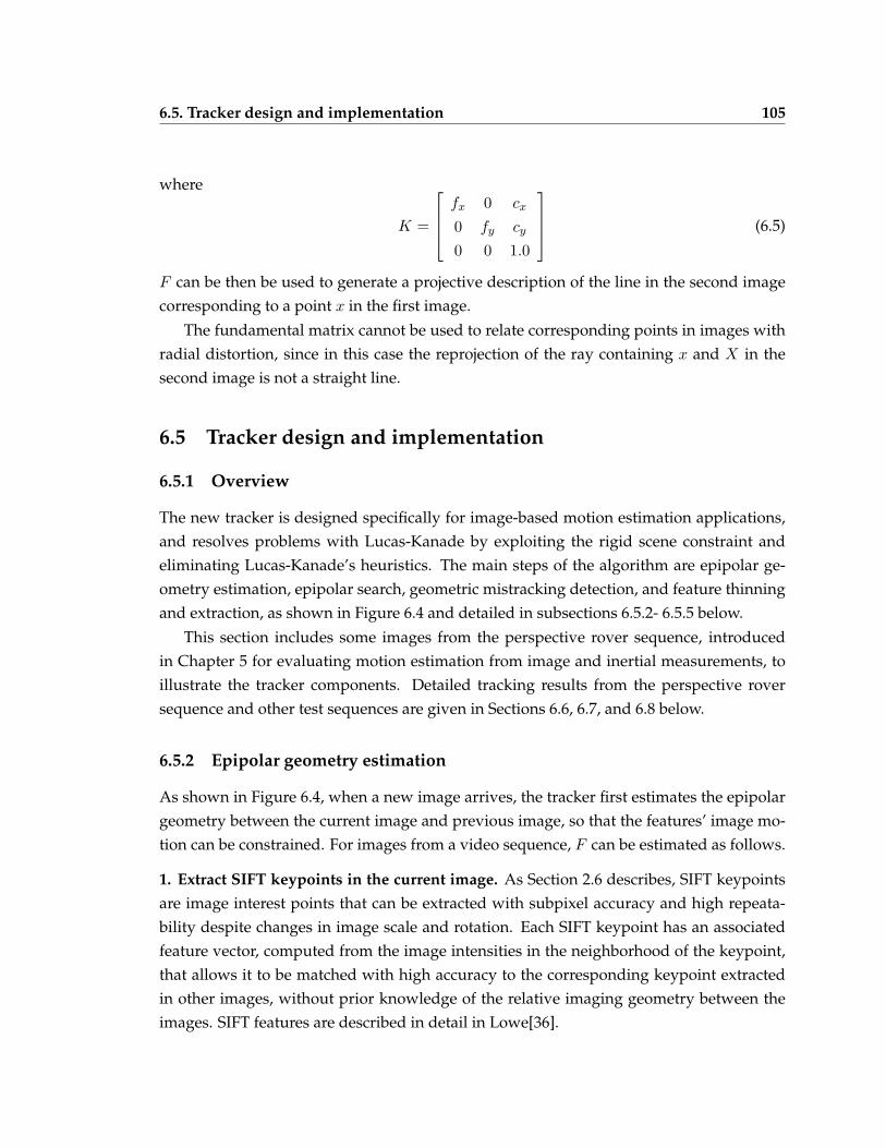
6.5. Tracker design and implementation 105
where
K =
fx 0 cx
0 fy cy
0 0 1.0
(6.5)
F can be then be used to generate a projective description of the line in the second imagecorresponding to a point x in the first image.
The fundamental matrix cannot be used to relate corresponding points in images withradial distortion, since in this case the reprojection of the ray containing x and X in thesecond image is not a straight line.
6.5 Tracker design and implementation
6.5.1 Overview
The new tracker is designed specifically for image-based motion estimation applications,and resolves problems with Lucas-Kanade by exploiting the rigid scene constraint andeliminating Lucas-Kanade’s heuristics. The main steps of the algorithm are epipolar ge-ometry estimation, epipolar search, geometric mistracking detection, and feature thinningand extraction, as shown in Figure 6.4 and detailed in subsections 6.5.2- 6.5.5 below.
This section includes some images from the perspective rover sequence, introducedin Chapter 5 for evaluating motion estimation from image and inertial measurements, toillustrate the tracker components. Detailed tracking results from the perspective roversequence and other test sequences are given in Sections 6.6, 6.7, and 6.8 below.
6.5.2 Epipolar geometry estimation
As shown in Figure 6.4, when a new image arrives, the tracker first estimates the epipolargeometry between the current image and previous image, so that the features’ image mo-tion can be constrained. For images from a video sequence, F can be estimated as follows.
1. Extract SIFT keypoints in the current image. As Section 2.6 describes, SIFT keypointsare image interest points that can be extracted with subpixel accuracy and high repeata-bility despite changes in image scale and rotation. Each SIFT keypoint has an associatedfeature vector, computed from the image intensities in the neighborhood of the keypoint,that allows it to be matched with high accuracy to the corresponding keypoint extractedin other images, without prior knowledge of the relative imaging geometry between theimages. SIFT features are described in detail in Lowe[36].
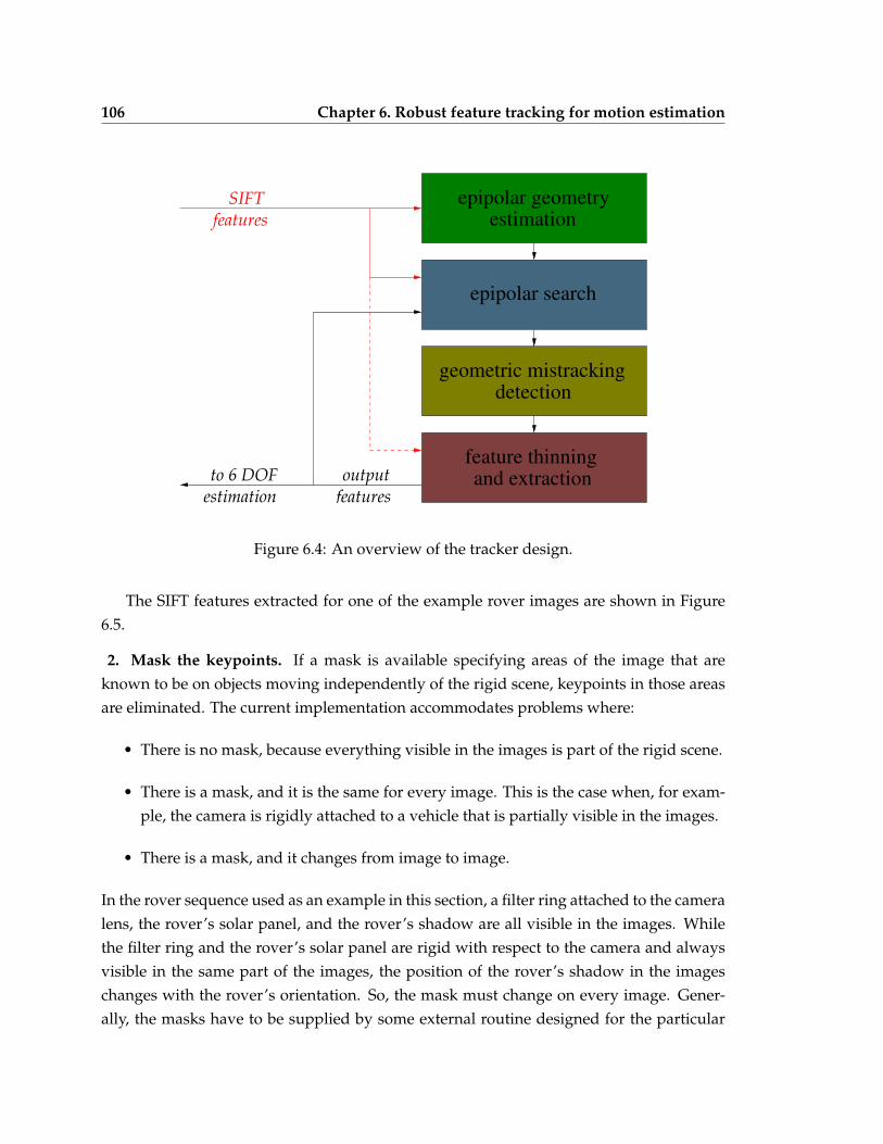
106 Chapter 6. Robust feature tracking for motion estimation
epipolar search
geometric mistrackingdetection
estimationepipolar geometry
featuresoutput
featuresSIFT
estimationto 6 DOF and extraction
feature thinning
Figure 6.4: An overview of the tracker design.
The SIFT features extracted for one of the example rover images are shown in Figure6.5.
2. Mask the keypoints. If a mask is available specifying areas of the image that areknown to be on objects moving independently of the rigid scene, keypoints in those areasare eliminated. The current implementation accommodates problems where:
• There is no mask, because everything visible in the images is part of the rigid scene.
• There is a mask, and it is the same for every image. This is the case when, for exam-ple, the camera is rigidly attached to a vehicle that is partially visible in the images.
• There is a mask, and it changes from image to image.
In the rover sequence used as an example in this section, a filter ring attached to the cameralens, the rover’s solar panel, and the rover’s shadow are all visible in the images. Whilethe filter ring and the rover’s solar panel are rigid with respect to the camera and alwaysvisible in the same part of the images, the position of the rover’s shadow in the imageschanges with the rover’s orientation. So, the mask must change on every image. Gener-ally, the masks have to be supplied by some external routine designed for the particular
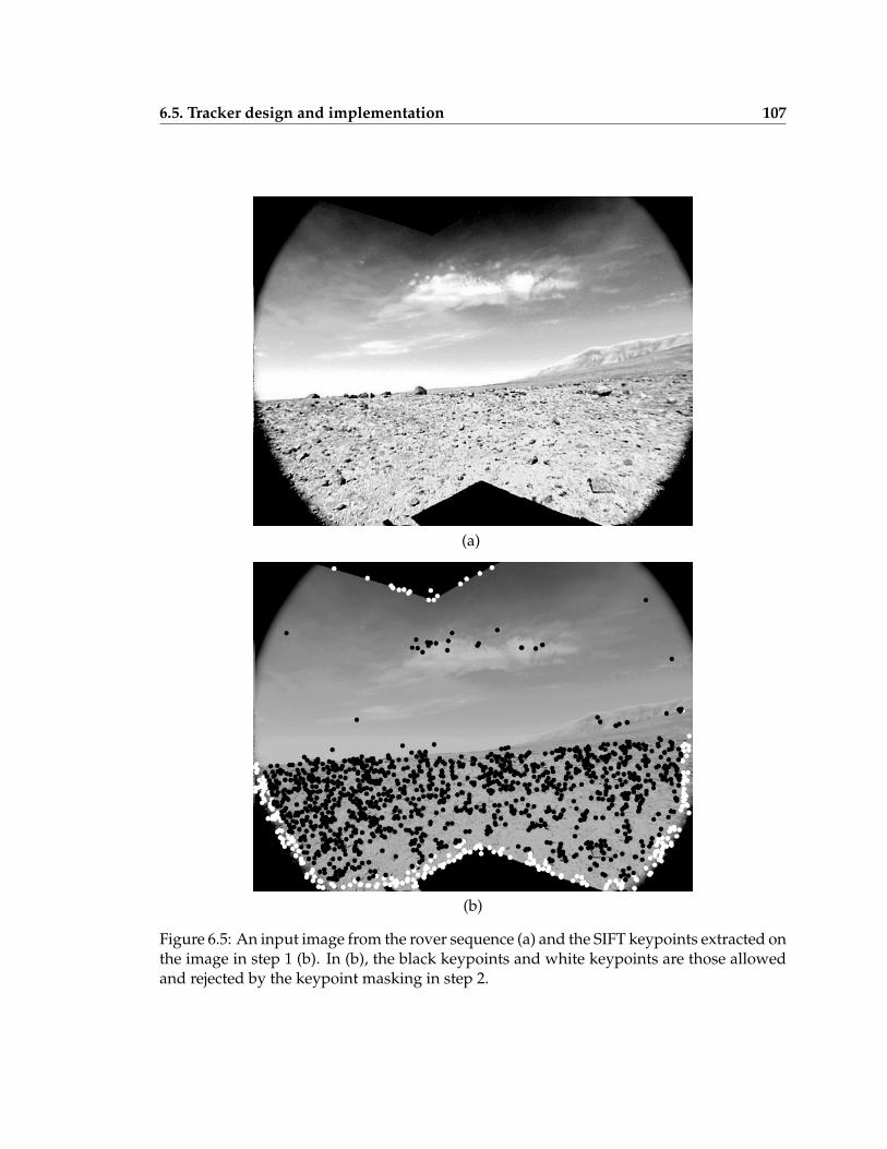
6.5. Tracker design and implementation 107
(a)
(b)
Figure 6.5: An input image from the rover sequence (a) and the SIFT keypoints extracted onthe image in step 1 (b). In (b), the black keypoints and white keypoints are those allowedand rejected by the keypoint masking in step 2.
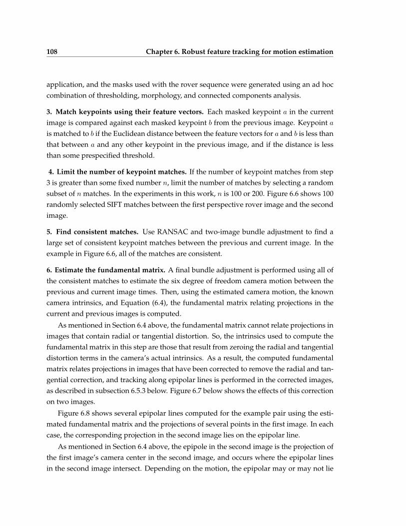
108 Chapter 6. Robust feature tracking for motion estimation
application, and the masks used with the rover sequence were generated using an ad hoccombination of thresholding, morphology, and connected components analysis.
3. Match keypoints using their feature vectors. Each masked keypoint a in the currentimage is compared against each masked keypoint b from the previous image. Keypoint a
is matched to b if the Euclidean distance between the feature vectors for a and b is less thanthat between a and any other keypoint in the previous image, and if the distance is lessthan some prespecified threshold.
4. Limit the number of keypoint matches. If the number of keypoint matches from step3 is greater than some fixed number n, limit the number of matches by selecting a randomsubset of n matches. In the experiments in this work, n is 100 or 200. Figure 6.6 shows 100randomly selected SIFT matches between the first perspective rover image and the secondimage.
5. Find consistent matches. Use RANSAC and two-image bundle adjustment to find alarge set of consistent keypoint matches between the previous and current image. In theexample in Figure 6.6, all of the matches are consistent.
6. Estimate the fundamental matrix. A final bundle adjustment is performed using all ofthe consistent matches to estimate the six degree of freedom camera motion between theprevious and current image times. Then, using the estimated camera motion, the knowncamera intrinsics, and Equation (6.4), the fundamental matrix relating projections in thecurrent and previous images is computed.
As mentioned in Section 6.4 above, the fundamental matrix cannot relate projections inimages that contain radial or tangential distortion. So, the intrinsics used to compute thefundamental matrix in this step are those that result from zeroing the radial and tangentialdistortion terms in the camera’s actual intrinsics. As a result, the computed fundamentalmatrix relates projections in images that have been corrected to remove the radial and tan-gential correction, and tracking along epipolar lines is performed in the corrected images,as described in subsection 6.5.3 below. Figure 6.7 below shows the effects of this correctionon two images.
Figure 6.8 shows several epipolar lines computed for the example pair using the esti-mated fundamental matrix and the projections of several points in the first image. In eachcase, the corresponding projection in the second image lies on the epipolar line.
As mentioned in Section 6.4 above, the epipole in the second image is the projection ofthe first image’s camera center in the second image, and occurs where the epipolar linesin the second image intersect. Depending on the motion, the epipolar may or may not lie
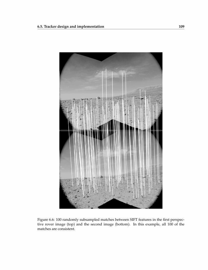
6.5. Tracker design and implementation 109
Figure 6.6: 100 randomly subsampled matches between SIFT features in the first perspec-tive rover image (top) and the second image (bottom). In this example, all 100 of thematches are consistent.
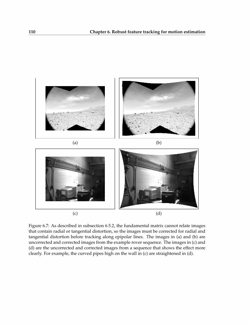
110 Chapter 6. Robust feature tracking for motion estimation
(a) (b)
(c) (d)
Figure 6.7: As described in subsection 6.5.2, the fundamental matrix cannot relate imagesthat contain radial or tangential distortion, so the images must be corrected for radial andtangential distortion before tracking along epipolar lines. The images in (a) and (b) areuncorrected and corrected images from the example rover sequence. The images in (c) and(d) are the uncorrected and corrected images from a sequence that shows the effect moreclearly. For example, the curved pipes high on the wall in (c) are straightened in (d).
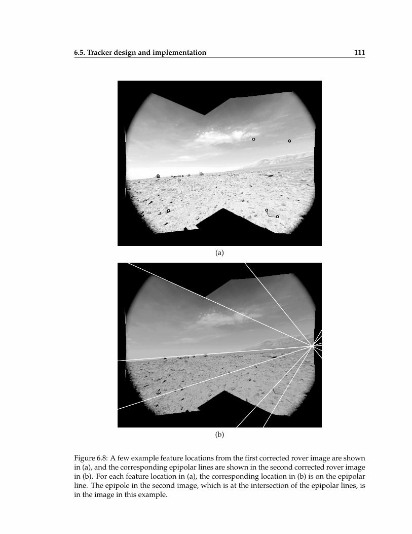
6.5. Tracker design and implementation 111
(a)
(b)
Figure 6.8: A few example feature locations from the first corrected rover image are shownin (a), and the corresponding epipolar lines are shown in the second corrected rover imagein (b). For each feature location in (a), the corresponding location in (b) is on the epipolarline. The epipole in the second image, which is at the intersection of the epipolar lines, isin the image in this example.
112 Chapter 6. Robust feature tracking for motion estimation
within the image. For the motion estimated between the two example images, the epipoleis in the image, as shown in the figure.
As mentioned in subsection 6.1, using SIFT to estimate the epipolar geometry is ad-vantageous in that SIFT makes no problematic assumptions on the image motion. Forinstance, SIFT does not place any a priori limit on the size of the motion, or assume thatthe motion is continuous or translational.
6.5.3 Epipolar search
Once the fundamental matrix relating the two undistorted images has been recovered, thelocations of features in the current image are found by a one-dimensional search alongtheir epipolar lines, as described in this subsection. This is the second box in Figure 6.4.
The following steps are used to perform the one-dimensional search.
1. Get an initial position. Get an initial position in the new image for each tracked pointby taking an average of the motion of the inlier SIFT keypoints from the previous step. Theterms in the average are weighted by the inverse distance of the SIFT keypoint’s positionin the first image from the tracked point’s position in the first image.
Points whose resulting initial positions are outside of the image, or whose templatefrom the previous image would overlap with the invalid mask if placed at the initial esti-mate, are marked as invalid and removed from the tracking process. This prevents pointsfrom latching onto objects in the image that are not part of the rigid scene.
2. Perform a discrete search. For each surviving feature, project the features’s initial po-sition found in step 1 onto the features’s epipolar line in the current image. Then, searchdiscrete locations along the epipolar line on each side of this projected location for thesum-of-squared-differences minimum between the feature’s intensity template from theprevious image and the intensities in the current image.
The existing implementation uses 60 locations on each side of the projected location in1 pixel increments, and a 41 × 41 pixel feature template from the previous image, for thediscrete search. The initial estimates generated from SIFT matches in step 1 above may ormay not be accurate depending on the amount of parallax in the scene and the distancefrom the tracked feature to the nearest SIFT keypoints, so the resulting 120 pixel searchrange is not overly conservative. The large 41 × 41 template sizes are chosen to eliminateambiguity in the matching.
As in the previous step, features whose resulting positions are outside of the image, orwhose template from the previous image would overlap with the invalid mask if placed at
6.5. Tracker design and implementation 113
the initial estimate, are marked as invalid and removed from the tracking process.
3. Perform a subpixel search. To get the feature’s location to subpixel accuracy, performa one-dimensional Lucas-Kanade search along the epipolar line, starting from the discreteminimum found in the previous step.
In the current implementation, a 21×21 pixel template is used for the one-dimensionalLucas-Kanade search.
6.5.4 Geometric mistracking detection
As shown in Figure 6.4, the third component of the tracker is geometric mistracking detec-tion.
Once the features have been tracked into the current image using one-dimensionalsearch, RANSAC and bundle adjustment are used to identify the largest set of featuresthat appear in the most recent three images, and whose tracked locations in those imagesare consistent with some choice of six degree of freedom camera positions for those imagesand three-dimensional point positions for the tracked features. Features that appeared inthe three most recent images and are not consistent with this set of feature locations areidentified as mistracked, and removed from the tracking process starting with the currentimage.
6.5.5 Feature thinning and extraction
As shown in Figure 6.4, the final step of the tracker is feature thinning and extraction.
1. Feature thinning. As features are tracked through the image sequence, their relativepositions in the image will change, and if new features are extracted in newly visible partsof the scene as the sequence progresses, an arbitrarily large number of features may ac-cumulate in one part of the image. For instance, if the camera is moving backward alongits optical axis, tracked points will group together at the center of the image. Tracking allof these grouped points is impractical, and for the purposes of camera motion estimation,tracking all of these points is not necessary, since the information these points provide isnearly redundant.
So, features that have survived geometric mistracking detection are thinned by elimi-nating features whose locations in the current image are within some threshold distance ofthe location of an older surviving feature. Removing younger features is preferred becauseolder features are likely to be more valuable in estimating the camera position relative tothe camera’s start position.

114 Chapter 6. Robust feature tracking for motion estimation
2. Feature extraction. As the image sequence progresses, new areas of the scene will be-come visible, and already visible parts of the scene may become featureless as mistrackedfeatures are detected and eliminated. So, feature extraction is performed in each image bychoosing features in areas of the current image that are featureless after thinning.
As mentioned in Section 6.1, feature extraction is based on two observations:
• Large fields of view are beneficial for estimating six degree of freedom camera mo-tion, but to exploit the large field of view it is necessary to track features throughoutthe entire view.
• Constraining feature tracking to the feature’s epipolar lines in the current imagemakes tracking less sensitive to poor, repetitive, or one-dimensional texture thanunconstrained tracking.
So, the feature extraction works by choosing features that are at least some distance fromany existing feature, and as a secondary criterion, have some minimal texture.
In the current implementation, the SIFT keypoint locations are used as the candidatefeature locations, because SIFT keypoints tend to be extracted wherever there is some min-imal texture in the images, as shown in Figure 6.5(b). However, this is not a fundamentalchoice, and any features that satisfy these two criteria would be acceptable choices. This isindicated by the dashed line in Figure 6.4.
To prevent newly extracted points from being thinned in the very next image, thethreshold distance for thinning should be smaller than that for extraction. 15 and 25 pixelsare typical thresholds for thinning and extraction, respectively.
6.6 Results Overview
The tracker’s behavior has been evaluated on five image sequences, which differ in:
• camera configuration
• amount of translational and rotational camera motion
• scene planarity or nonplanarity, and range of scene depths
• image conditions, such as amount and type of texture, occlusions, and specularities
The five sequences are:
6.6. Results Overview 115
• Rover. This sequence includes the first 200 images from the perspective rover se-quence examined in the previous chapter. The images are 640 × 480, taken from anIEEE 1394 camera with a wide field of view lens, mounted on a manually controlledrover.
The camera motion for this sequence is roughly planar translation in x, y and rotationabout the camera’s y (image up) axis. The scene includes roughly planar terrain inthe foreground, with mountains and the sky at infinity, and contains a mix of welltextured and weakly textured areas.
• Highbay. This sequence includes 200 640 × 480 images taken from an IEEE 1394camera with a wide field of view lens, mounted on a manually controlled cart.
Like the rover sequence, the camera motion for this sequence is planar translation inx, y and rotation about the camera’s y (image up) axis. The scene is highly non-planarand well textured in most areas. The resulting sequence includes occlusions.
• Helicopter. This sequence includes 200 640 × 480 images taken from an IEEE 1394camera with a wide field of view lens, mounted on a remote control helicopter.
The camera motion in this sequence contains translation in x and y, a lesser trans-lation in z, and rotation about the camera’s optical axis. The scene is planar, andincludes a mix of well textured and weakly textured areas. The images contain se-vere compression artifacts.
• Crane. This sequence contains 200 images selected from the perspective crane se-quence examined in Chapter 5. The images are 640 × 240, taken from a CCD camerawith a narrow field of view lens, mounted on a computer controlled crane.
The camera motion includes significant translational motion in x, y, and z, but onlyvery minor rotational motion. The scene is highly nonplanar, well textured every-where, and contains repetitive texture, one-dimensional texture, and specularities.The resulting image sequence contains many occlusions.
• Arm. This sequence is the perspective arm sequence examined in Chapter 5. Thesequence includes 152 640 × 240 images taken from a CCD camera with a narrowfield of view lens, mounted on a computer controlled arm.
The camera motion includes significant translational motion in x, y, and z and signif-icant rotational motion about the camera’s z (optical) axis. The scene is planar, andcontains repetitive, weak, and one-dimensional texture.
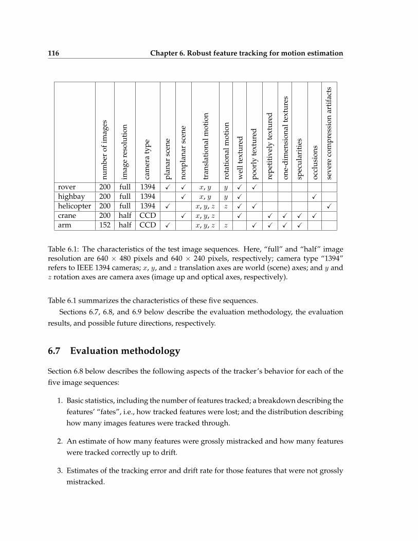
116 Chapter 6. Robust feature tracking for motion estimation
num
ber
ofim
ages
imag
ere
solu
tion
cam
era
type
plan
arsc
ene
nonp
lana
rsc
ene
tran
slat
iona
lmot
ion
rota
tion
alm
otio
n
wel
ltex
ture
d
poor
lyte
xtur
ed
repe
titi
vely
text
ured
one-
dim
ensi
onal
text
ures
spec
ular
itie
s
occl
usio
ns
seve
reco
mpr
essi
onar
tifa
cts
rover 200 full 1394 X X x, y y X X
highbay 200 full 1394 X x, y y X X
helicopter 200 full 1394 X x, y, z z X X X
crane 200 half CCD X x, y, z X X X X X
arm 152 half CCD X x, y, z z X X X X
Table 6.1: The characteristics of the test image sequences. Here, “full” and “half” imageresolution are 640 × 480 pixels and 640 × 240 pixels, respectively; camera type “1394”refers to IEEE 1394 cameras; x, y, and z translation axes are world (scene) axes; and y andz rotation axes are camera axes (image up and optical axes, respectively).
Table 6.1 summarizes the characteristics of these five sequences.
Sections 6.7, 6.8, and 6.9 below describe the evaluation methodology, the evaluationresults, and possible future directions, respectively.
6.7 Evaluation methodology
Section 6.8 below describes the following aspects of the tracker’s behavior for each of thefive image sequences:
1. Basic statistics, including the number of features tracked; a breakdown describing thefeatures’ “fates”, i.e., how tracked features were lost; and the distribution describinghow many images features were tracked through.
2. An estimate of how many features were grossly mistracked and how many featureswere tracked correctly up to drift.
3. Estimates of the tracking error and drift rate for those features that were not grosslymistracked.
6.7. Evaluation methodology 117
This section briefly describes how each of these statistics is computed.
6.7.1 Feature fates
For 1, tracked features are subject to four fates. Three of these fates are for lost features,which can be thinned, leave the field of view, or be eliminated because of geometric incon-sistency. The fourth fate is survival until the end of the sequence.
6.7.2 Estimating correct feature positions
For 2 and 3, estimates of the correct feature positions are needed. These are found by (1)estimating each feature’s three-dimensional position from estimates of the camera positionat the time of each image and from the tracked features and (2) reprojecting the three-dimensional position back into the images using the camera position estimates.
Two different approaches to computing the reprojections have been used. In the first,the observation covariance associated with a feature in the first image in which it is visibleis set very low, and the observation covariances are set normally for all subsequent images.As a result, the reprojection for the first image is the same as the observed projection, andthe reprojection error is distributed across the remaining features, but not necessarily inthe increasing “drifting” manner that is likely to be the real errors’ behavior. The estimatedtracking errors that result from these reprojections serve as an approximate lower boundon the real tracking errors. In the text below, reprojections computed using this methodare called “1 covariance” reprojections.
In the second, the observation covariance for the first image is set very low, the co-variances for the next nine images slightly higher, and the covariances for all subsequentimages are set normally. In this scenario, the reprojection for the first image is the sameas the observed projection, reprojection errors for the next nine images are not necessarily“drifting”, and the reprojection errors for all subsequent images are likely to exhibit thecorrect “drifting” behavior. The tracking error estimates computed from these reprojec-tions are likely to be closer to the true tracking error than the 1-covariance reprojections.These reprojections are called the “10 covariances” reprojections in the text below.
A third method, “2 covariances”, was also tried. In this method, the first observa-tion covariance is set very low, the second observation covariance was set slightly higher,and all subsequent covariances were set normally. Using these covariances, the first andsecond reprojection are nearly the same as the first two observed projections, and thethree-dimensional point position is essentially triangulated using the first two observa-tions. However, this method uses too little data and often results in poor reprojection
118 Chapter 6. Robust feature tracking for motion estimation
estimates.For the rover, highbay, helicopter, and crane image sequences, the camera position
estimates were found by supplying the tracking data to a variable state dimension filterequipped with aggressive outlier detection. In the arm sequence, the camera position esti-mates are the “?” image-and-inertial batch estimates described in subsection 5.3.3.
6.7.3 Identifying grossly mistracked features
For 2, features whose tracking errors only increase or decrease slowly are identified asdrifting features, whereas features whose tracking errors change more than some fixednumber of pixels between any two images are identified as grossly mistracked features.Here, the tracking errors are treated as two-dimensional, directional errors rather thanscalars. So, for example, the change in error of a feature that is observed three pixels belowits correct position in one image and three pixels above its correct position in the secondimage is 6.0 pixels, rather than 0.0 pixels.
Three different levels of gross mistracking have been explored, corresponding to 3.0,6.0, and 9.0 pixel thresholds for the change in error. The 3.0 pixel threshold is the most rea-sonable and, for brevity, detailed results have only been reported below for this threshold.The other thresholds are useful for identifying those features that exhibit the most severemistracking.
6.7.4 Drift estimates
For 3, tracking errors are summarized for those features that are identified as drifting.Drift rate statistics are also given, which normalize the reprojection error with the numberof images since the feature was first visible.
6.8 Evaluation
Table 6.2 gives the basic statistics describing the tracker behavior for each of the five testsequences. The first five entries of the table show how many features were tracked in eachsequence (row 1), the fates of those features that were eliminated during tracking (rows 2,3, and 4), and the number of features that were tracked until the end of the sequence (row5). Rows 6-9 summarize the distribution describing the number of images the featureswere tracked through. For instance, 25% of the features tracked in the rover sequencewere tracked through 16 images of more, and one of those features was tracked through167 images.
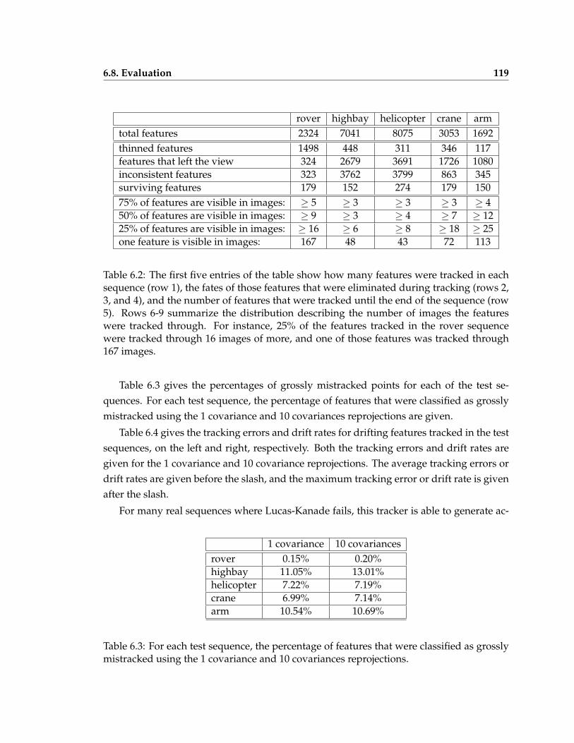
6.8. Evaluation 119
rover highbay helicopter crane armtotal features 2324 7041 8075 3053 1692thinned features 1498 448 311 346 117features that left the view 324 2679 3691 1726 1080inconsistent features 323 3762 3799 863 345surviving features 179 152 274 179 15075% of features are visible in images: ≥ 5 ≥ 3 ≥ 3 ≥ 3 ≥ 450% of features are visible in images: ≥ 9 ≥ 3 ≥ 4 ≥ 7 ≥ 1225% of features are visible in images: ≥ 16 ≥ 6 ≥ 8 ≥ 18 ≥ 25one feature is visible in images: 167 48 43 72 113
Table 6.2: The first five entries of the table show how many features were tracked in eachsequence (row 1), the fates of those features that were eliminated during tracking (rows 2,3, and 4), and the number of features that were tracked until the end of the sequence (row5). Rows 6-9 summarize the distribution describing the number of images the featureswere tracked through. For instance, 25% of the features tracked in the rover sequencewere tracked through 16 images of more, and one of those features was tracked through167 images.
Table 6.3 gives the percentages of grossly mistracked points for each of the test se-quences. For each test sequence, the percentage of features that were classified as grosslymistracked using the 1 covariance and 10 covariances reprojections are given.
Table 6.4 gives the tracking errors and drift rates for drifting features tracked in the testsequences, on the left and right, respectively. Both the tracking errors and drift rates aregiven for the 1 covariance and 10 covariance reprojections. The average tracking errors ordrift rates are given before the slash, and the maximum tracking error or drift rate is givenafter the slash.
For many real sequences where Lucas-Kanade fails, this tracker is able to generate ac-
1 covariance 10 covariancesrover 0.15% 0.20%highbay 11.05% 13.01%helicopter 7.22% 7.19%crane 6.99% 7.14%arm 10.54% 10.69%
Table 6.3: For each test sequence, the percentage of features that were classified as grosslymistracked using the 1 covariance and 10 covariances reprojections.
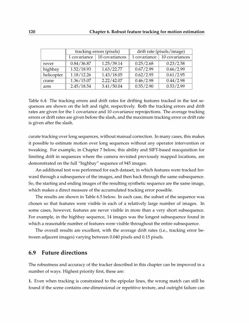
120 Chapter 6. Robust feature tracking for motion estimation
tracking errors (pixels) drift rate (pixels/image)1 covariance 10 covariances 1 covariance 10 covariances
rover 0.84/36.87 1.25/39.14 0.25/2.68 0.23/2.58highbay 1.52/18.93 1.63/22.77 0.67/2.99 0.66/2.99helicopter 1.18/12.26 1.43/18.05 0.62/2.95 0.61/2.95crane 1.36/15.07 2.22/42.07 0.46/2.98 0.44/2.98arm 2.45/18.54 3.41/50.04 0.55/2.90 0.53/2.99
Table 6.4: The tracking errors and drift rates for drifting features tracked in the test se-quences are shown on the left and right, respectively. Both the tracking errors and driftrates are given for the 1 covariance and 10 covariance reprojections. The average trackingerrors or drift rates are given before the slash, and the maximum tracking error or drift rateis given after the slash.
curate tracking over long sequences, without manual correction. In many cases, this makesit possible to estimate motion over long sequences without any operator intervention ortweaking. For example, in Chapter 7 below, this ability and SIFT-based reacquisition forlimiting drift in sequences where the camera revisited previously mapped locations, aredemonstrated on the full “highbay” sequence of 945 images.
An additional test was performed for each dataset, in which features were tracked for-ward through a subsequence of the images, and then back through the same subsequence.So, the starting and ending images of the resulting synthetic sequence are the same image,which makes a direct measure of the accumulated tracking error possible.
The results are shown in Table 6.5 below. In each case, the subset of the sequence waschosen so that features were visible in each of a relatively large number of images. Insome cases, however, features are never visible in more than a very short subsequence.For example, in the highbay sequence, 14 images was the longest subsequence found inwhich a reasonable number of features were visible throughout the entire subsequence.
The overall results are excellent, with the average drift rates (i.e., tracking error be-tween adjacent images) varying between 0.040 pixels and 0.15 pixels.
6.9 Future directions
The robustness and accuracy of the tracker described in this chapter can be improved in anumber of ways. Highest priority first, these are:
1. Even when tracking is constrained to the epipolar lines, the wrong match can still befound if the scene contains one-dimensional or repetitive texture, and outright failure can
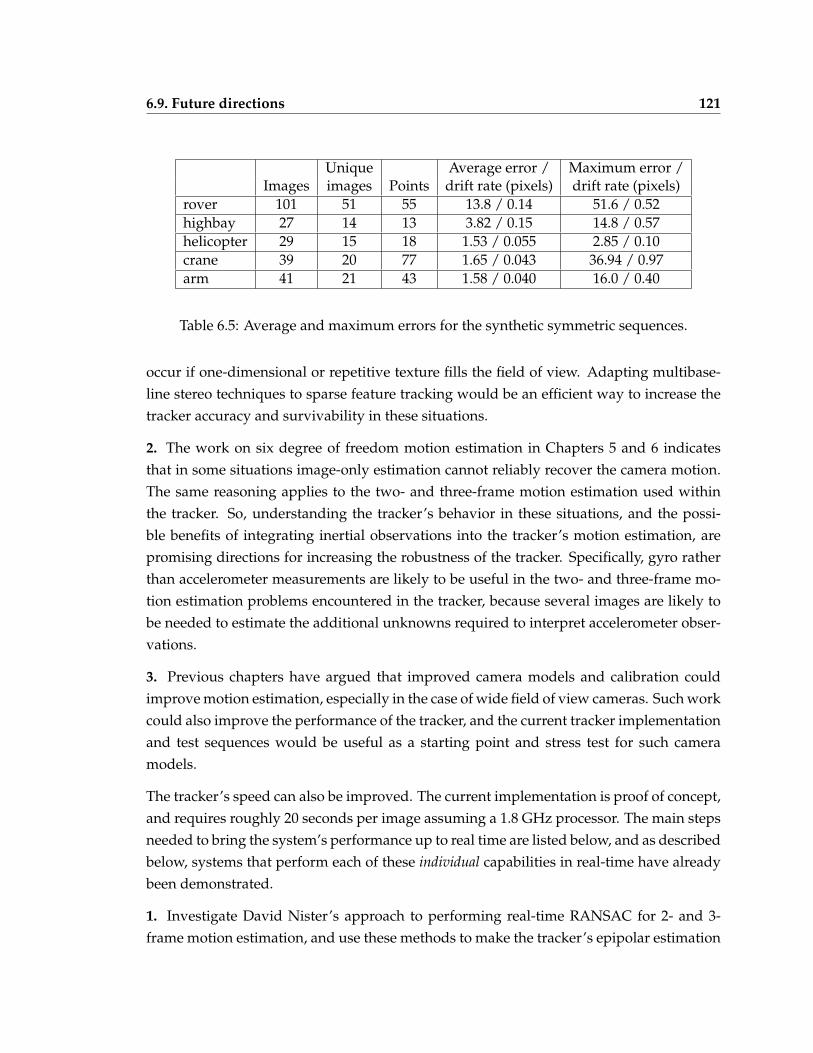
6.9. Future directions 121
Unique Average error / Maximum error /Images images Points drift rate (pixels) drift rate (pixels)
rover 101 51 55 13.8 / 0.14 51.6 / 0.52highbay 27 14 13 3.82 / 0.15 14.8 / 0.57helicopter 29 15 18 1.53 / 0.055 2.85 / 0.10crane 39 20 77 1.65 / 0.043 36.94 / 0.97arm 41 21 43 1.58 / 0.040 16.0 / 0.40
Table 6.5: Average and maximum errors for the synthetic symmetric sequences.
occur if one-dimensional or repetitive texture fills the field of view. Adapting multibase-line stereo techniques to sparse feature tracking would be an efficient way to increase thetracker accuracy and survivability in these situations.
2. The work on six degree of freedom motion estimation in Chapters 5 and 6 indicatesthat in some situations image-only estimation cannot reliably recover the camera motion.The same reasoning applies to the two- and three-frame motion estimation used withinthe tracker. So, understanding the tracker’s behavior in these situations, and the possi-ble benefits of integrating inertial observations into the tracker’s motion estimation, arepromising directions for increasing the robustness of the tracker. Specifically, gyro ratherthan accelerometer measurements are likely to be useful in the two- and three-frame mo-tion estimation problems encountered in the tracker, because several images are likely tobe needed to estimate the additional unknowns required to interpret accelerometer obser-vations.
3. Previous chapters have argued that improved camera models and calibration couldimprove motion estimation, especially in the case of wide field of view cameras. Such workcould also improve the performance of the tracker, and the current tracker implementationand test sequences would be useful as a starting point and stress test for such cameramodels.
The tracker’s speed can also be improved. The current implementation is proof of concept,and requires roughly 20 seconds per image assuming a 1.8 GHz processor. The main stepsneeded to bring the system’s performance up to real time are listed below, and as describedbelow, systems that perform each of these individual capabilities in real-time have alreadybeen demonstrated.
1. Investigate David Nister’s approach to performing real-time RANSAC for 2- and 3-frame motion estimation, and use these methods to make the tracker’s epipolar estimation
122 Chapter 6. Robust feature tracking for motion estimation
and geometric consistency RANSAC procedures real-time. These RANSAC proceduresare the dominant computational expense, so this is the highest priority.
2. Optimize the radial distortion correction, the discrete epipolar line search, and the sub-pixel epipolar line search to achieve real-time performance. Real-time stereo systems havebeen demonstrated that perform radial distortion correction and rectification, and densetracking of the features along epipolar lines in real-time. Tracking along epipolar lines inimage streams differs from real-time stereo in that rectification of adjacent images in thevideo stream, to align the epipolar lines with raster lines, is not practical for general cam-era motion. However, tracking in the context of motion from images requires sparse ratherthan dense tracking, so rectification is probably not needed to achieve real-time perfor-mance.
3. Implement real-time SIFT feature extraction and matching. Real-time SIFT feature ex-traction and matching has already been demonstrated in a commercial product.
Chapter 7
Long-term motion estimation
7.1 Overview
As discussed in the previous chapters, existing systems are not suitable for the long-termmotion estimation problems that arise in autonomous vehicle navigation and modelingfrom video, because they are susceptible to both gross local errors and long-term drift.Chapters 2-6 have investigated omnidirectional images, image and inertial measurements,and constrained tracking. Although the addition of an accelerometer to image-based mo-tion estimation can provide two components of the sensors’ orientation without drift, themethods described in these previous chapters are primarily concerned with reducing grosslocal errors in the estimated motion.
This chapter considers the problem of long-term drift directly. Limiting drift in caseswhere the camera revisits a previously mapped location requires:
• Recognizing from the images that a previously mapped location has been revisited.
• Using observations of the revisited location to reduce drift in the estimated positions.
The second problem has been extensively studied in the SLAM community, whereas rec-ognizing a previously mapped location from images is unique to image-based motion es-timation.
This chapter describes a proof of concept system for long-term motion that addressesthese two problems, by exploiting the tracker described in the previous chapter, the vari-able state dimension filter (VSDF), and SIFT keypoints. This system is described in detailin Section 7.2 below, and the system’s performance on a long image sequence in which thecamera repeatedly revisits locations is described in Section 7.3. Section 7.4 discusses theremaining issues.
123
124 Chapter 7. Long-term motion estimation
7.2 Method
Like many systems for estimating motion from images, the system estimates the currentcamera position using two steps. When a new image arrives, features are first tracked inthe new image using the tracker described in Chapter 6. The resulting feature locations arethen passed to a variable state dimension filter (VSDF) that estimates the camera positionat the time of the new image, and the three-dimensional positions of the tracked points.
However, the system may also be able to generate a motion estimate for the currentcamera position with lower error by recognizing a previously mapped location, and ex-tending an archived rollback state corresponding to that location. The following subsectionsdescribe this process in detail.
The variable state dimension filter, used for six degree of freedom motion estimation inthe system, is a hybrid batch-recursive algorithm, described in detail by McLauchlan[38]in the context of shape and motion estimation from image measurements. Chapters 2 and4 above have already suggested extending the VSDF for estimating sensor motion fromimage and inertial measurements. However, the VSDF used here is an image-only filter,extended to identify mistracked features using RANSAC.
SIFT keypoints are an enabling technology for recognizing previously mapped loca-tions. SIFT keypoints are reviewed briefly in Section 2.6, and described in detail by Lowe[36].
7.2.1 Active state
An active state Si describes the system after processing the most recent image, with indexi. The structure of the active state is shown in Figure 7.1. The active state contains a listof image indices, I . During the system’s initial operation, I will be the set of sequentialindices 0, . . . , i. As we’ll see below, however, I is not generally this sequential set.
The active state also contains an instance of the tracker described in Chapter 6. Thistracker instance gives a history of sparse, two-dimensional feature locations found bytracking through the image sequence I . Similarly, the active state contains an instanceof the variable state dimension filter that includes six degree of freedom position and errorcovariance estimates for the camera at the time of each image in I , and estimates of thethree-dimensional point positions of the features that were tracked through the images inI . Last, the active state also contains the SIFT keypoints extracted in the most recent image,as shown in the figure.
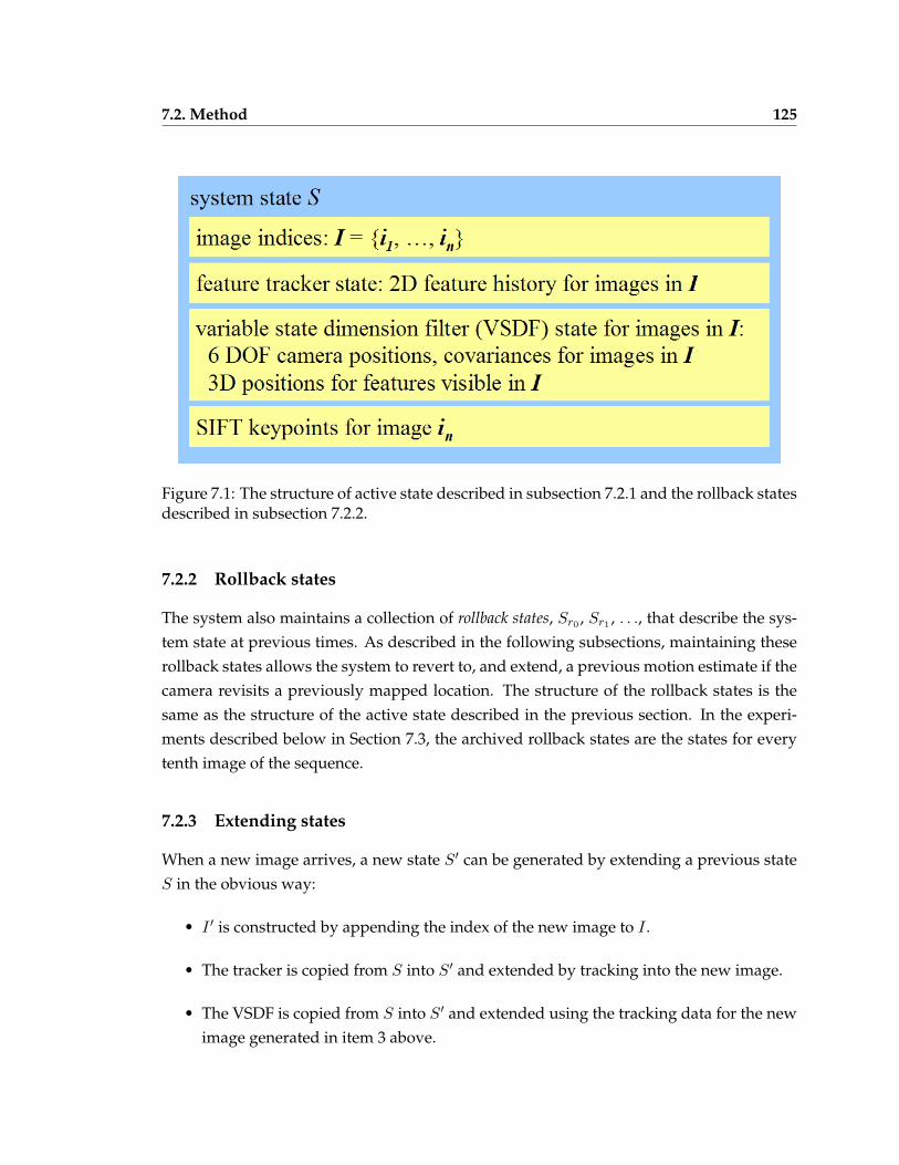
7.2. Method 125
Figure 7.1: The structure of active state described in subsection 7.2.1 and the rollback statesdescribed in subsection 7.2.2.
7.2.2 Rollback states
The system also maintains a collection of rollback states, Sr0 , Sr1 , . . ., that describe the sys-tem state at previous times. As described in the following subsections, maintaining theserollback states allows the system to revert to, and extend, a previous motion estimate if thecamera revisits a previously mapped location. The structure of the rollback states is thesame as the structure of the active state described in the previous section. In the experi-ments described below in Section 7.3, the archived rollback states are the states for everytenth image of the sequence.
7.2.3 Extending states
When a new image arrives, a new state S′ can be generated by extending a previous stateS in the obvious way:
• I ′ is constructed by appending the index of the new image to I .
• The tracker is copied from S into S′ and extended by tracking into the new image.
• The VSDF is copied from S into S′ and extended using the tracking data for the newimage generated in item 3 above.
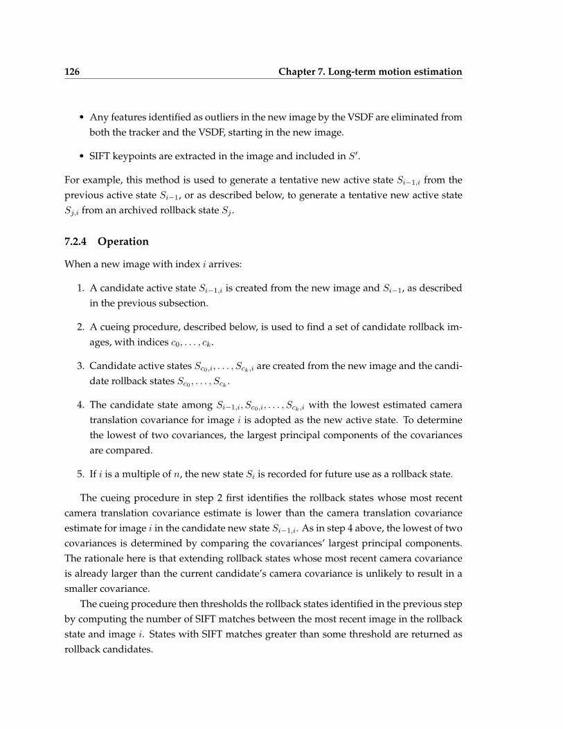
126 Chapter 7. Long-term motion estimation
• Any features identified as outliers in the new image by the VSDF are eliminated fromboth the tracker and the VSDF, starting in the new image.
• SIFT keypoints are extracted in the image and included in S′.
For example, this method is used to generate a tentative new active state Si−1,i from theprevious active state Si−1, or as described below, to generate a tentative new active stateSj,i from an archived rollback state Sj .
7.2.4 Operation
When a new image with index i arrives:
1. A candidate active state Si−1,i is created from the new image and Si−1, as describedin the previous subsection.
2. A cueing procedure, described below, is used to find a set of candidate rollback im-ages, with indices c0, . . . , ck.
3. Candidate active states Sc0,i, . . . , Sck,i are created from the new image and the candi-date rollback states Sc0 , . . . , Sck
.
4. The candidate state among Si−1,i, Sc0,i, . . . , Sck,i with the lowest estimated cameratranslation covariance for image i is adopted as the new active state. To determinethe lowest of two covariances, the largest principal components of the covariancesare compared.
5. If i is a multiple of n, the new state Si is recorded for future use as a rollback state.
The cueing procedure in step 2 first identifies the rollback states whose most recentcamera translation covariance estimate is lower than the camera translation covarianceestimate for image i in the candidate new state Si−1,i. As in step 4 above, the lowest of twocovariances is determined by comparing the covariances’ largest principal components.The rationale here is that extending rollback states whose most recent camera covarianceis already larger than the current candidate’s camera covariance is unlikely to result in asmaller covariance.
The cueing procedure then thresholds the rollback states identified in the previous stepby computing the number of SIFT matches between the most recent image in the rollbackstate and image i. States with SIFT matches greater than some threshold are returned asrollback candidates.
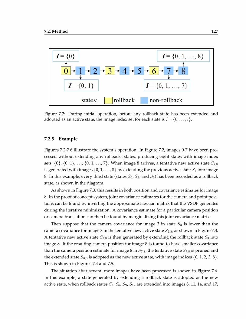
7.2. Method 127
Figure 7.2: During initial operation, before any rollback state has been extended andadopted as an active state, the image index set for each state is I = {0, . . . , i}.
7.2.5 Example
Figures 7.2-7.6 illustrate the system’s operation. In Figure 7.2, images 0-7 have been pro-cessed without extending any rollbacks states, producing eight states with image indexsets, {0}, {0, 1}, . . ., {0, 1, . . ., 7}. When image 8 arrives, a tentative new active state S7,8
is generated with images {0, 1, . . ., 8} by extending the previous active state S7 into image8. In this example, every third state (states S0, S3, and S6) has been recorded as a rollbackstate, as shown in the diagram.
As shown in Figure 7.3, this results in both position and covariance estimates for image8. In the proof of concept system, joint covariance estimates for the camera and point posi-tions can be found by inverting the approximate Hessian matrix that the VSDF generatesduring the iterative minimization. A covariance estimate for a particular camera positionor camera translation can then be found by marginalizing this joint covariance matrix.
Then suppose that the camera covariance for image 3 in state S3 is lower than thecamera covariance for image 8 in the tentative new active state S7,8, as shown in Figure 7.3.A tentative new active state S3,8 is then generated by extending the rollback state S3 intoimage 8. If the resulting camera position for image 8 is found to have smaller covariancethan the camera position estimate for image 8 in S7,8, the tentative state S7,8 is pruned andthe extended state S3,8 is adopted as the new active state, with image indices {0, 1, 2, 3, 8}.This is shown in Figures 7.4 and 7.5.
The situation after several more images have been processed is shown in Figure 7.6.In this example, a state generated by extending a rollback state is adopted as the newactive state, when rollback states S3, S6, S9, S12 are extended into images 8, 11, 14, and 17,
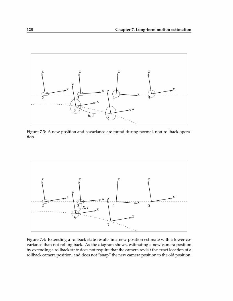
128 Chapter 7. Long-term motion estimation
z
x
2
z
z z z
x
x
xx
8
3 4 5
z
x
7R, t
Figure 7.3: A new position and covariance are found during normal, non-rollback opera-tion.
z
x
2
z
z z z
x
x
xx
8
3 4
z
x
7
5R, t
Figure 7.4: Extending a rollback state results in a new position estimate with a lower co-variance than not rolling back. As the diagram shows, estimating a new camera positionby extending a rollback state does not require that the camera revisit the exact location of arollback camera position, and does not “snap” the new camera position to the old position.
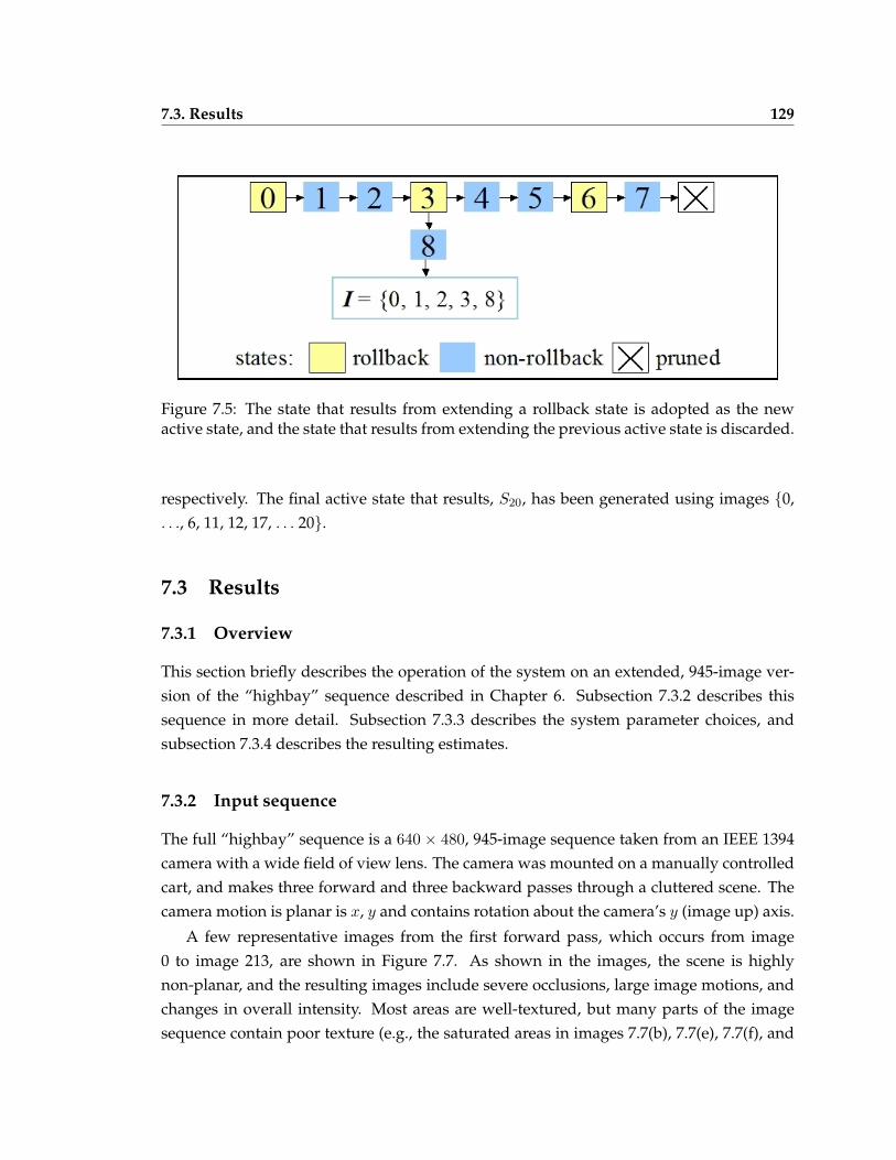
7.3. Results 129
Figure 7.5: The state that results from extending a rollback state is adopted as the newactive state, and the state that results from extending the previous active state is discarded.
respectively. The final active state that results, S20, has been generated using images {0,. . ., 6, 11, 12, 17, . . . 20}.
7.3 Results
7.3.1 Overview
This section briefly describes the operation of the system on an extended, 945-image ver-sion of the “highbay” sequence described in Chapter 6. Subsection 7.3.2 describes thissequence in more detail. Subsection 7.3.3 describes the system parameter choices, andsubsection 7.3.4 describes the resulting estimates.
7.3.2 Input sequence
The full “highbay” sequence is a 640 × 480, 945-image sequence taken from an IEEE 1394camera with a wide field of view lens. The camera was mounted on a manually controlledcart, and makes three forward and three backward passes through a cluttered scene. Thecamera motion is planar is x, y and contains rotation about the camera’s y (image up) axis.
A few representative images from the first forward pass, which occurs from image0 to image 213, are shown in Figure 7.7. As shown in the images, the scene is highlynon-planar, and the resulting images include severe occlusions, large image motions, andchanges in overall intensity. Most areas are well-textured, but many parts of the imagesequence contain poor texture (e.g., the saturated areas in images 7.7(b), 7.7(e), 7.7(f), and
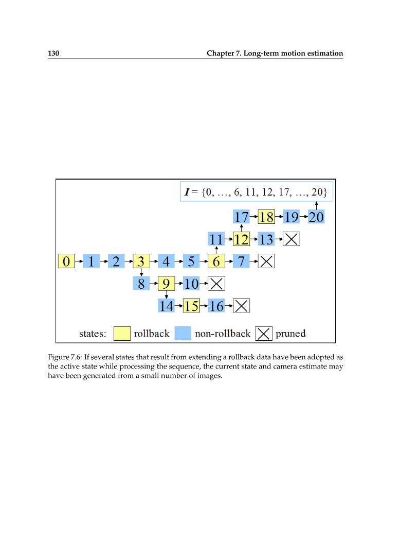
130 Chapter 7. Long-term motion estimation
Figure 7.6: If several states that result from extending a rollback data have been adopted asthe active state while processing the sequence, the current state and camera estimate mayhave been generated from a small number of images.
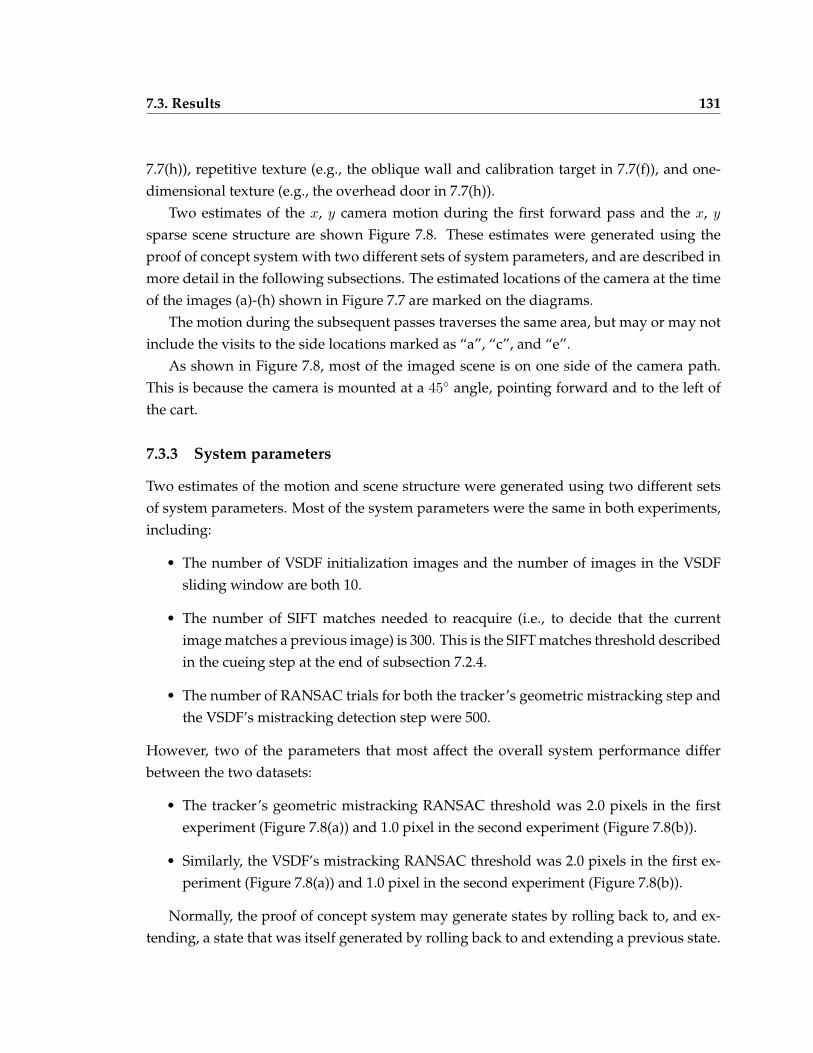
7.3. Results 131
7.7(h)), repetitive texture (e.g., the oblique wall and calibration target in 7.7(f)), and one-dimensional texture (e.g., the overhead door in 7.7(h)).
Two estimates of the x, y camera motion during the first forward pass and the x, y
sparse scene structure are shown Figure 7.8. These estimates were generated using theproof of concept system with two different sets of system parameters, and are described inmore detail in the following subsections. The estimated locations of the camera at the timeof the images (a)-(h) shown in Figure 7.7 are marked on the diagrams.
The motion during the subsequent passes traverses the same area, but may or may notinclude the visits to the side locations marked as “a”, “c”, and “e”.
As shown in Figure 7.8, most of the imaged scene is on one side of the camera path.This is because the camera is mounted at a 45◦ angle, pointing forward and to the left ofthe cart.
7.3.3 System parameters
Two estimates of the motion and scene structure were generated using two different setsof system parameters. Most of the system parameters were the same in both experiments,including:
• The number of VSDF initialization images and the number of images in the VSDFsliding window are both 10.
• The number of SIFT matches needed to reacquire (i.e., to decide that the currentimage matches a previous image) is 300. This is the SIFT matches threshold describedin the cueing step at the end of subsection 7.2.4.
• The number of RANSAC trials for both the tracker’s geometric mistracking step andthe VSDF’s mistracking detection step were 500.
However, two of the parameters that most affect the overall system performance differbetween the two datasets:
• The tracker’s geometric mistracking RANSAC threshold was 2.0 pixels in the firstexperiment (Figure 7.8(a)) and 1.0 pixel in the second experiment (Figure 7.8(b)).
• Similarly, the VSDF’s mistracking RANSAC threshold was 2.0 pixels in the first ex-periment (Figure 7.8(a)) and 1.0 pixel in the second experiment (Figure 7.8(b)).
Normally, the proof of concept system may generate states by rolling back to, and ex-tending, a state that was itself generated by rolling back to and extending a previous state.
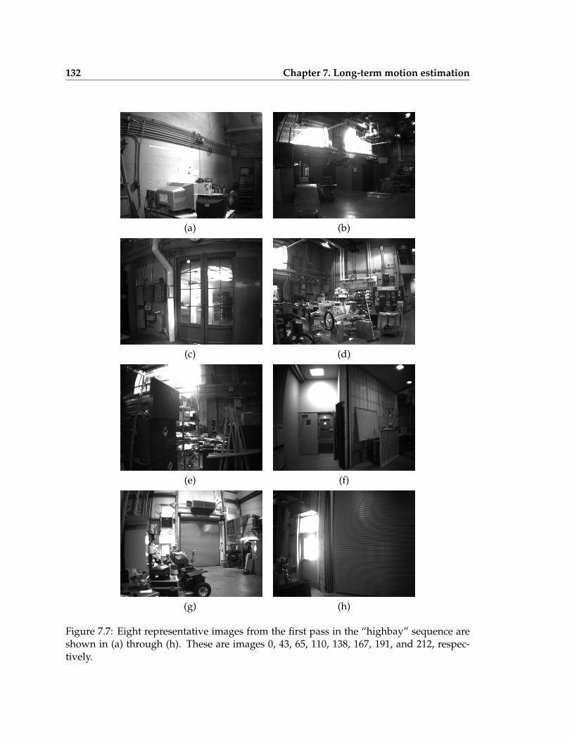
132 Chapter 7. Long-term motion estimation
(a) (b)
(c) (d)
(e) (f)
(g) (h)
Figure 7.7: Eight representative images from the first pass in the “highbay” sequence areshown in (a) through (h). These are images 0, 43, 65, 110, 138, 167, 191, and 212, respec-tively.
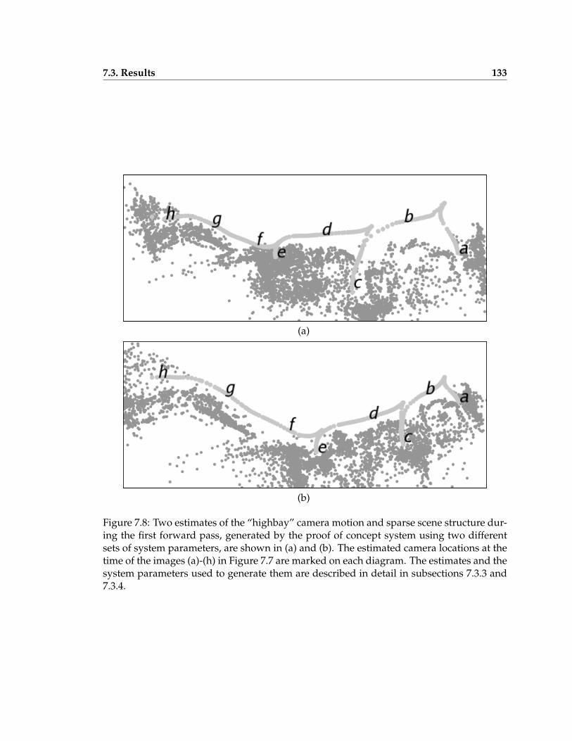
7.3. Results 133
(a)
(b)
Figure 7.8: Two estimates of the “highbay” camera motion and sparse scene structure dur-ing the first forward pass, generated by the proof of concept system using two differentsets of system parameters, are shown in (a) and (b). The estimated camera locations at thetime of the images (a)-(h) in Figure 7.7 are marked on each diagram. The estimates and thesystem parameters used to generate them are described in detail in subsections 7.3.3 and7.3.4.
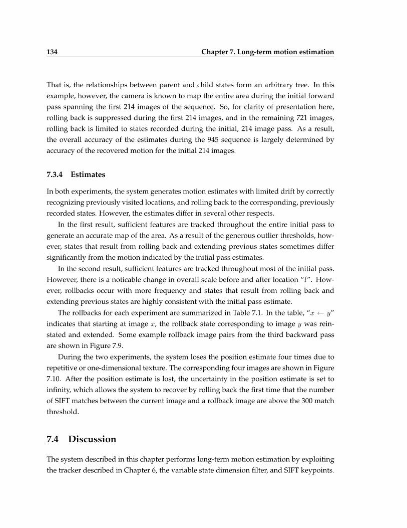
134 Chapter 7. Long-term motion estimation
That is, the relationships between parent and child states form an arbitrary tree. In thisexample, however, the camera is known to map the entire area during the initial forwardpass spanning the first 214 images of the sequence. So, for clarity of presentation here,rolling back is suppressed during the first 214 images, and in the remaining 721 images,rolling back is limited to states recorded during the initial, 214 image pass. As a result,the overall accuracy of the estimates during the 945 sequence is largely determined byaccuracy of the recovered motion for the initial 214 images.
7.3.4 Estimates
In both experiments, the system generates motion estimates with limited drift by correctlyrecognizing previously visited locations, and rolling back to the corresponding, previouslyrecorded states. However, the estimates differ in several other respects.
In the first result, sufficient features are tracked throughout the entire initial pass togenerate an accurate map of the area. As a result of the generous outlier thresholds, how-ever, states that result from rolling back and extending previous states sometimes differsignificantly from the motion indicated by the initial pass estimates.
In the second result, sufficient features are tracked throughout most of the initial pass.However, there is a noticable change in overall scale before and after location “f”. How-ever, rollbacks occur with more frequency and states that result from rolling back andextending previous states are highly consistent with the initial pass estimate.
The rollbacks for each experiment are summarized in Table 7.1. In the table, “x ← y”indicates that starting at image x, the rollback state corresponding to image y was rein-stated and extended. Some example rollback image pairs from the third backward passare shown in Figure 7.9.
During the two experiments, the system loses the position estimate four times due torepetitive or one-dimensional texture. The corresponding four images are shown in Figure7.10. After the position estimate is lost, the uncertainty in the position estimate is set toinfinity, which allows the system to recover by rolling back the first time that the numberof SIFT matches between the current image and a rollback image are above the 300 matchthreshold.
7.4 Discussion
The system described in this chapter performs long-term motion estimation by exploitingthe tracker described in Chapter 6, the variable state dimension filter, and SIFT keypoints.
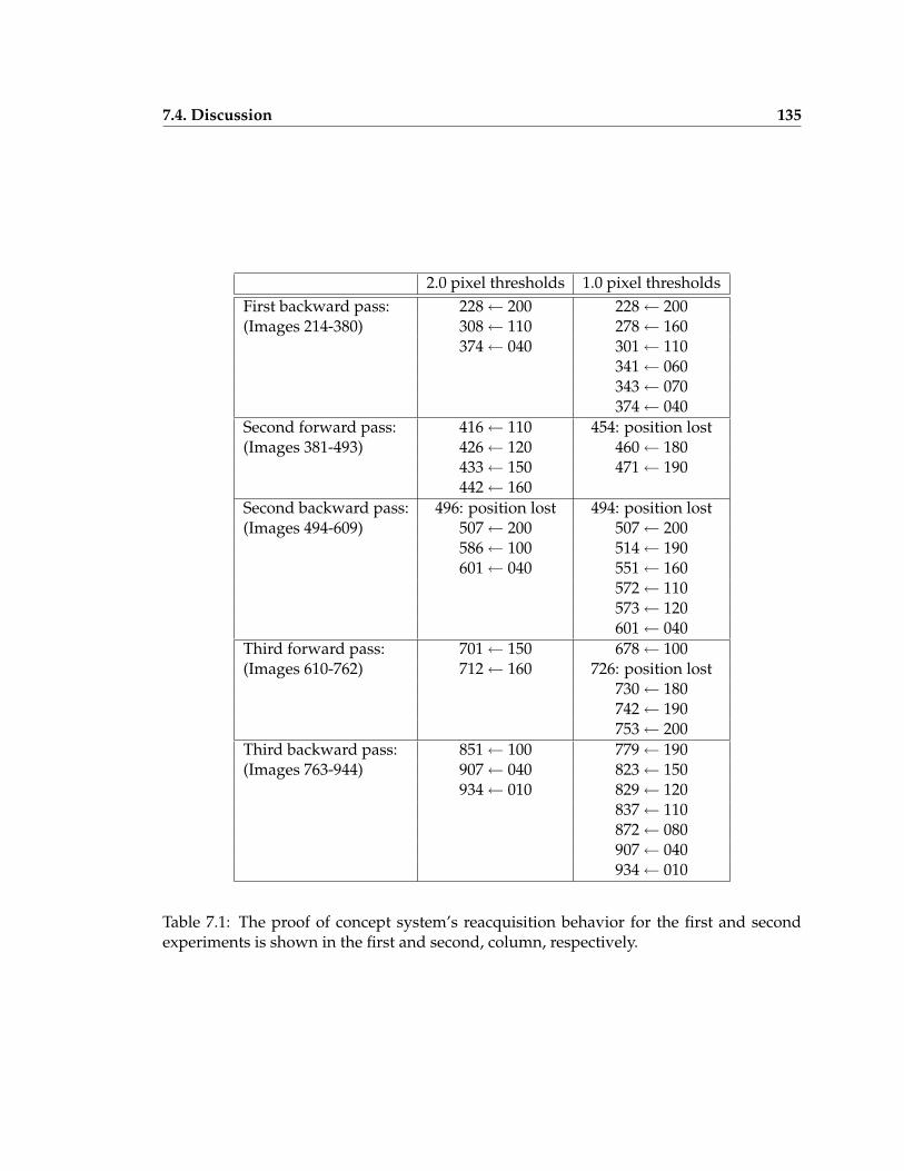
7.4. Discussion 135
2.0 pixel thresholds 1.0 pixel thresholdsFirst backward pass: 228← 200 228← 200(Images 214-380) 308← 110 278← 160
374← 040 301← 110341← 060343← 070374← 040
Second forward pass: 416← 110 454: position lost(Images 381-493) 426← 120 460← 180
433← 150 471← 190442← 160
Second backward pass: 496: position lost 494: position lost(Images 494-609) 507← 200 507← 200
586← 100 514← 190601← 040 551← 160
572← 110573← 120601← 040
Third forward pass: 701← 150 678← 100(Images 610-762) 712← 160 726: position lost
730← 180742← 190753← 200
Third backward pass: 851← 100 779← 190(Images 763-944) 907← 040 823← 150
934← 010 829← 120837← 110872← 080907← 040934← 010
Table 7.1: The proof of concept system’s reacquisition behavior for the first and secondexperiments is shown in the first and second, column, respectively.
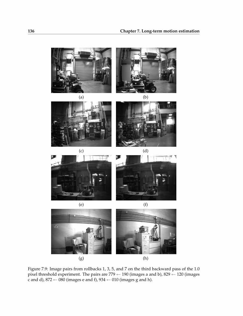
136 Chapter 7. Long-term motion estimation
(a) (b)
(c) (d)
(e) (f)
(g) (h)
Figure 7.9: Image pairs from rollbacks 1, 3, 5, and 7 on the third backward pass of the 1.0pixel threshold experiment. The pairs are 779← 190 (images a and b), 829← 120 (imagesc and d), 872← 080 (images e and f), 934← 010 (images g and h).
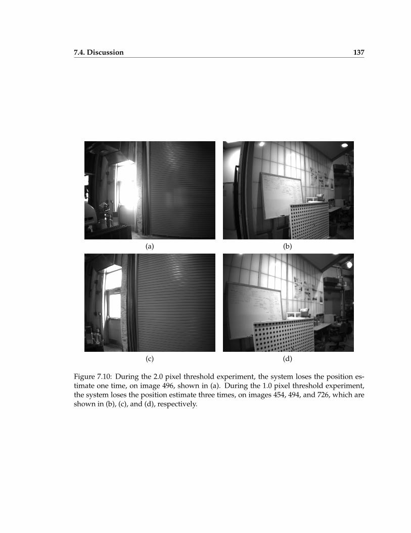
7.4. Discussion 137
(a) (b)
(c) (d)
Figure 7.10: During the 2.0 pixel threshold experiment, the system loses the position es-timate one time, on image 496, shown in (a). During the 1.0 pixel threshold experiment,the system loses the position estimate three times, on images 454, 494, and 726, which areshown in (b), (c), and (d), respectively.
138 Chapter 7. Long-term motion estimation
The system includes both capabilities that such a system needs: recognizing previouslyvisited locations and exploiting observations of previously visited locations for reducingthe errors in estimation.
However, the approaches to these two capabilities are just a starting point, and manyissues in deploying such a system for everyday use still remain. For instance, in the sys-tem as it is described here, the number of recorded rollback states grows linearly with thenumber of images in the sequence, and each recorded rollback state is large. This limi-tation might be mitigated by reducing the size of the individual recorded rollback states,by reducing the number of tracked points, by adopting a one-dimensional (i.e., depth)rather than a three-dimensional parameterization of the estimated feature positions, or byinvestigating a more space efficient invariant feature method to replace SIFT features.
However, in the existing system, cueing time increases with the linearly increasingnumber of rollback states, and reducing the size of the individual rollback states does notaddress this problem. To fix this more fundamental problem, two approaches are possible.First, methods to minimize the number of recorded rollback states while still providingadequate coverage of the explored area should be investigated. Second, more effectiveuse of the current camera position and covariances estimate should be made to reduce thenumber of recorded rollback states that are examined in full.
One difficulty specific to the first capability, recognizing previously visited locations,is that SIFT features cannot be matched across severe changes in scale and view angle.Both the system and the experimental data described in this chapter would be excellentstarting points for exploring additional approaches for efficiently recognizing landmarksacross more severe changes in scale and viewpoint, such as perceptual grouping.
The second capability, exploiting the recognition of a previously visited location, isaddressed in a straightforward way by this system, but the system does not include somecapabilities that have been investigated in the SLAM literature. For instance, efficientlyupdating the history of estimates, rather than just the most recent estimate, is requiredfor closing the loop and producing an accurate overall map. The system described in thischapter would be an excellent starting point for investigating these ideas in the context ofmotion from images.
As described in the paragraphs above, some additional capabilities should be investi-gated for inclusion in the system, but at the same time, the initial experiment described inSection 7.3 does not explore all of the system’s existing capabilities, and more experimentsshould be performed with the existing system. For example, the results in Section 7.3 weregenerating using a strict threshold on the number of SIFT matches between the currentimage and rollback images, but this strict threshold limits rollbacks to those states that are
7.4. Discussion 139
very close in viewpoint to the current image, as shown in Figure 7.9. The system is de-signed to correctly achieve and exploit rollbacks from more severe changes in viewpoint,and the system’s performance for different choices of this threshold parameter should beexplored in the future.
As a final observation, the system described in this chapter achieves long-term motionestimation by adding relatively simple components to a robust feature tracker, the variablestate dimension filter, and SIFT, and the quality of the resulting estimates is highly depen-dent on the quality of these components. Although the problems of tracking, six degreeof freedom motion estimation, and invariant image features have long been the subject ofresearch in the vision community, the performance of these subsystems is still the limitingfactor in the performance of the system described here.

Chapter 8
Conclusion
8.1 Overview
This work has focused on developing the robustness and accuracy needed to bring image-based motion estimation to long-term motion applications, such as autonomous vehiclenavigation and modeling from video. In particular, the work has focused on four areas:
• Modeling and calibration of noncentral omnidirectional cameras, and motion esti-mation from omnidirectional images using the resulting model.
• Exploiting the complementary nature of image and inertial measurements for robustmotion estimation.
• Making the robustness and accuracy of sparse image feature tracking meet the strin-gent requirements of motion estimation from real sequences.
• Exploiting feature reacquisition to limit drift in long-term motion estimation.
Sections 8.2, 8.4, and 8.5 below summarize the technical conclusions that can be drawnfrom this work, the contributions of this work, and possible future directions, respectively.
8.2 Conclusions
Some of the key conclusions that can be drawn from this work are:
1. Motion estimation from omnidirectional images benefits from a precise camera model,including the relative misalignment between the camera and mirror, even if the mis-alignment is slight. On the other hand, given a calibration, it is possible to perform
141
142 Chapter 8. Conclusion
accurate motion estimation even if the misalignment between the camera and mirroris severe.
2. One calibration image is sufficient to determine the misalignment between an omni-directional camera’s mirror and camera.
3. Motion from image measurements alone can be highly sensitive to both small errorsin the observed projections and to the camera intrinsics calibration.
4. Motion estimation from image and inertial measurements can produce accurate esti-mates even in cases where the estimates from image or inertial measurements aloneare poor. Measurements from inexpensive inertial sensors can serve to eliminatethe sensitivity that can occur in image-only estimation, estimate the global orienta-tion, and establish the global scale. Image measurements are beneficial in limitingthe drift that occurs in integrating inertial sensors, and make it possible estimate theunknowns that are needed to interpret inertial sensor outputs without any a prioriassumptions.
5. Using both image measurements and measurements from inexpensive inertial sen-sors primarily benefits local motion estimates, rather than long-term motion esti-mates. In the long term, accelerometers’ dependence on gravity can estimate twocomponents of the sensors’ global orientation without drift, but inexpensive inertialsensors are unlikely to eliminate gradual drift in azimuth or translation.
6. Omnidirectional images can provide some of the benefits of using both conventionalimage and inertial measurements, such as decreased sensitivity to very sparse ob-servations. Of course, some potential benefits that inertial sensors provide, such asrecovery of the global scale and the global orientation, cannot be recovered using justomnidirectional images.
7. Although they cannot be used for real-time or ”infinite” operation, batch algorithmsare an important tool for motion estimation. Estimates from these algorithms aresometimes useful in their own right. In other applications, the batch estimate is im-portant in understanding the best quality we can expect given a particular sensorconfiguration, vehicle motion, environment, and set of observations, and in mea-suring the inherent sensitivity of the estimate with respect to random observationerrors.
8. In both image-only and image-and-inertial estimation, the iterated extended Kalmanfilter (IEKF) can be made to work for long-term camera motion estimation given suf-
8.3. Recommendations 143
ficiently accurate image measurements. However, (1) the IEKF can be highly sensi-tive to the camera motion propagation variances, and (2) assuming the state containsonly the current camera position, the IEKF does not model the relative errors betweenadjacent camera positions.
9. Exploiting the rigid scene assumption and eliminating the heuristics often used withsparse feature tracking can produce highly reliable, dense feature tracking suitablefor camera motion estimation.
10. The position of a camera moving between a number of locations over a long timeperiod can be estimated with limited drift using feature reacquisition and relativelysimple extensions to feature tracking and recursive motion estimation.
8.3 Recommendations
As described in Section 8.1, this work has examined four approaches to improving motionfrom image measurements. This section includes some comments on the relative merits ofthese approaches, and some explicit recommendations for exploiting them in combination.
Chapter 5 explores the relative advantages of motion from omnidirectional images andof motion from conventional images and inertial measurements, and in the experimentsin that chapter, the advantages over conventional images alone only are roughly the samein each case. However, the advantages of omnidirectional cameras are more limited inpractice:
• The potential strength of omnidirectional images for motion estimation largely re-sults from scene points being visible in more of the image sequence as the camerachanges its view angle. In the case of a camera that sees 360◦ in azimuth and 180◦
in elevation, and moves in a convex environment, every point is visible all the time.However, most omnidirectional cameras do not see 180◦ in elevation, and most en-vironments are not convex and contain occlusions, so this advantage is limited inmost cases. Furthermore, points may not always be trackable in the omnidirectionalimage even if they are visible, further limiting the number of images in which theyare useful for motion estimation.
• Omnidirectional images are susceptible to overexposure. The sun causes saturationoutdoors, and overhead lights cause saturation indoors.
• As mentioned above, most omnidirectional cameras do provide a 180◦ view in ele-vation. 90 − 140◦ might be more typical values. In this case, a wide field of view
144 Chapter 8. Conclusion
conventional camera that provides 70− 80◦ in elevation (i.e., 140− 160◦ total field ofview) would provide many of the advantages of an omnidirectional camera with theconvenience of a conventional projection model.
• Feature tracking is more difficult in omnidirectional images than in conventionalimages.
• Motion from omnidirectional images alone cannot recover the global scale or estab-lish components of the rotation without drift, whereas image and inertial measure-ments together can.
In short, motion from wide field of view, conventional image measurements and inertialmeasurements is preferable to motion from omnidirectional images in practice.
Chapter 5 also illustrates that image and inertial measurements can reduce sensitivityto tracking and camera calibration errors, but initial experiments in which six degree offreedom motion is estimated using a wide field of view camera and the tracker describedin Chapter 6 indicate that these also significantly increase accuracy. However, neither ofthese is ideal alone. Accurate tracking is still needed to perform motion from image andinertial measurements; and motion from dense, accurate tracking alone cannot provide theglobal scale or estimate components of the rotation without drift, even in the best case.
Feature reacquisition, as described in Chapter 7, provides an advantage that none ofthe other approaches provide, i.e., limiting drift in the case where the camera revisits pre-viously mapped locations. However, even when using reacquisition the accuracy of theoverall map is limited by the accuracy of raw motion estimation when no revisition occursand a loop cannot be closed. So, all efforts should be made to maximize the accuracy ofmotion estimation in the absence of reacquisition. In the context of the current system, thiswould entail incorporating inertial measurements into the existing, image-only system forlong-term motion estimation described in Chapter 7.
8.4 Contributions
1. A general catadioptric projection model was developed, which can accommodatenoncentral cameras and misalignment between the omnidirectional rig’s camera andmirror. Existing batch and recursive algorithms for simultaneously estimating cam-era motion and sparse scene structure were extended to omnidirectional camerasusing this projection model.
8.4. Contributions 145
2. An algorithm was developed to determine the mirror-to-camera calibration requiredfor item (1) from a single image of known three-dimensional points. It was shownthat this calibration accurately recovers the mirror-to-camera transformation, allowsaccurate shape-from-motion and epipolar matching even when the camera and mir-ror are severely misaligned, and increases shape-from-motion and epipolar matchingaccuracy even when the camera and mirror are closely aligned.
3. A batch algorithm for estimating sensor motion and sparse scene structure and fromimage, gyro, and accelerometer measurements was developed, which requires no apriori assumptions or limits on the sensor motion or scene structure. The optimalestimates produced by this algorithm are useful in their own right, and as a goldstandard for the comparison of online algorithms.
4. A recursive, IEKF-based algorithm for estimating sensor motion and sparse scenestructure from image, gyro, and accelerometer measurements was developed. Thisalgorithm is a multirate method, meaning that separate measurement update stepsare used to incorporate the image and inertial measurements at the different rates atwhich they become available. The requirements for correctly initializing newly visi-ble points in the IEKF framework were analyzed, and a method for initializing newpoints, adapted from the simultaneous localization and mapping (SLAM) commu-nity, was introduced.
5. Using a large suite of experimental results, this work has attempted to establish fun-damental facts about motion estimation from image and inertial measurements, andto evaluate the performance of the specific algorithms described here.
6. An algorithm for tracking sparse image features for motion estimation was devel-oped that greatly improves on the accuracy of Lucas-Kanade, the previous go-totracker in the shape-from-motion community. This algorithm exploits the rigid sceneassumption and SIFT keypoints, and eliminates the poor heuristics normally used fortracking sparse features.
7. A system was developed for simultaneously estimating the long-term motion of acamera that revisits points in a finite scene, and the sparse structure of that envi-ronment. In problems where the camera revisits previously mapped locations, thissystem is able to limit long-term drift.
146 Chapter 8. Conclusion
8.5 Future directions
The system developed in this work would benefit from further work on a number of topics,which are described in this section. In each case, the existing system would provide anexcellent starting point for investigation, and the experimental results from the existingsystem would set a high bar for evaluating new developments.
The IEKF-based recursive method for estimating motion from image and inertial mea-surements is limited by the inability to model the relative errors between adjacent cameraestimates, the implicit assumption of motion smoothness, the approximation of the stateestimate by a Gaussian, and the linearization of measurements around uncertain state es-timates. As suggested in previous chapters, these problems can be eliminated or mitigatedusing the variable state dimension filter (VSDF), so a priority for future work should bethe construction of a VSDF for estimating motion from image and inertial measurementsbased on the batch algorithm presented in this work.
Because the covariance between currently visible points and points that are no longervisible is not modeled in the current recursive algorithm, the recursive algorithm cannotimprove previously estimated states based on observations of revisited points. This capa-bility would be useful for closing the loop and improving the overall accuracy of motionestimates. Techniques for closing the loop from the simultaneous localization and map-ping (SLAM) literature, which investigates this problem in the context of ground roverswith range sensors and odometry, would be a good starting point for this improvement.
The system described in Chapter 7 for long-term motion estimation uses a simple tech-nique for recognizing previously visited locations that requires time linear in the numberof images seen so far. More efficient techniques for fast recognition would be beneficial andthe system developed in this work would be a good platform for evaluating such work.
The conventional camera model used in this work appears to be an important limitingfactor in the accuracy of the system over the long term. Nonparametric and noncentralmodels for conventional cameras are a promising approach to increasing the accuracy ofthe camera model, and would also allow very-wide-angle conventional cameras (i.e., con-ventional cameras with fields of view near 180◦) to be modeled and incorporated into thissystem.
The accuracy of the inertial sensors used in this work appears to be limited by theassumed sensor models rather than the random noise in the sensor outputs. The batch al-gorithm for motion from image and inertial measurements developed in this work wouldbe an excellent platform for developing and evaluating more sophisticated models of thesesensors’ behavior.
8.5. Future directions 147
Like previous work in shape-from-motion, this work has assumed that the observationerrors between projections for the same point in different images, and for different pointsin the same image, are uncorrelated. However, this is clearly not the case. For instance, theuse of a common epipolar geometry for constraining the projections of different points inthe same image introduces related errors in these projections. On the other hand, image-to-image tracking introduces a drift in projections for the same point in different imagesover time. Modeling the correlation between projection errors and efficiently incorporatingthe resulting model into motion estimation are both challenging problems that could beinvestigated in the context of this work.

Bibliography
[1] Simon Baker and Shree K. Nayar. A theory of single-viewpoint catadioptric imageformation. International Journal of Computer Vision, 35(2):1–22, 1999.
[2] Yaakov Bar-Shalom and Xiao-Rong Li. Multitarget-Multisensor Tracking: Principles andTechniques. YBS Publishing, Storrs, Connecticut, 1995.
[3] J. M. Bradshaw, M. Sierhuis, Y. Gawdiak, R. Jeffers, N. Suri, and M. Greaves. Ad-justable autonomy and teamwork for the personal satellite assistant. In IJCAI-01Workshop on Autonomy, Delegation, and Control: Interacting with Autonomous Agents,Seattle, Washington, August 2001.
[4] Jeffrey M. Bradshaw, Maarten Sierhuis, Yuri Gawdiak, Hans Thomas, Mark Greaves,and William J. Clancy. Human-centered design for the personal satellite assistant.In International Conference on Human-Computer Interaction in Aeronautics, Toulouse,France, 2000.
[5] T. J. Broida, S. Chandrashekhar, and R. Chellappa. Recursive 3-D motion estimationfrom a monocular image sequence. IEEE Transactions on Aerospace and Electronic Sys-tems, 26(4):639–656, July 1990.
[6] Ted J. Broida and Rama Chellappa. Performance bounds for estimating three-dimensional motion parameters from a sequence of noisy images. Journal of the OpticalSociety of America A, 6(6):879–889, June 1989.
[7] Michael J. Brooks, Wojciech Chojnacki, Darren Gawley, and Anton van den Hengel.What value covariance information in estimating vision parameters? In Eighth IEEEInternational Conference on Computer Vision (ICCV 2001), Vancouver, Canada, 2001.
[8] J. S. Chahl and M. V. Srinivasan. Reflective surfaces for panoramic imaging. AppliedOptics, 36(31):8275–8285, 1997.
149
150 BIBLIOGRAPHY
[9] Lin Chai, William A. Hoff, and Tyrone Vincent. Three-dimensional motion and struc-ture estimation using inertial sensors and computer vision for augmented reality.Presence, 11(5):474–491, 2002.
[10] John J. Craig. Introduction to Robotics: Mechanics and Control. Addison-Wesley, Read-ing, Massachusetts, 1989.
[11] Matthew Deans and Martial Hebert. Experimental comparison of techniques for lo-calization and mapping using a bearing-only sensor. In Daniela Rus and Sanjiv Singh,editors, Experimental Robotics VII, pages 395–404. Springer-Verlag, Berlin, 2001.
[12] Matthew C. Deans. Bearings-only localization and mapping. PhD thesis, Carnegie MellonUniversity, Pittsburgh, Pennsylvania, 2002.
[13] S.F. El-Hakim. 3D modeling of complex environments. In SPIE Proceedings, ElectronicImaging 2001, Volume 4309: Videometrics and Optical Methods for 3D Shape MeasurementVII, San Jose, California, January 2001.
[14] Eric Foxlin and Leonid Naimark. VIS-Tracker: A wearable vision-inertial self-tracker.In IEEE Virtual Reality Conference (VR 2003), Los Angeles, March 2003.
[15] Eric M. Foxlin. Generalized architecture for simultaneous localization, auto-calibration, and map-building. In IEEE/RSJ Conference on Intelligent Robots and Systems(IROS 2002), Lausanne, Switzerland, October 2002.
[16] Arthur Gelb, editor. Applied Optimal Estimation. MIT Press, Cambridge, Mas-sachusetts, 1974.
[17] Christopher Geyer and Kostas Daniilidis. Catadioptric camera calibration. In SeventhIEEE International Conference on Computer Vision (ICCV 1999), pages 398–404, Septem-ber 1999.
[18] Christopher Geyer and Kostas Daniilidis. Catadioptric projective geometry. Interna-tional Journal of Computer Vision, December 2001.
[19] Christopher Geyer and Kostas Daniilidis. Structure and motion from uncalibratedcatadioptric views. IEEE Conference on Computer Vision and Pattern Recognition (CVPR2001), December 2001.
[20] Christopher Geyer and Kostas Daniilidis. Paracatadioptric camera calibration. IEEETransactions on Pattern Analysis and Machine Intelligence (PAMI), 24(5), May 2002.
BIBLIOGRAPHY 151
[21] Christopher Geyer and Kostas Daniilidis. Conformal rectification of an omnidirec-tional stereo pair. In Proceedings of the Omnidirectional Workshop and Sensor Networks(OMNIVIS 2003), Madison, Wisconsin, June 2003.
[22] Christopher Geyer and Kostas Daniilidis. Mirrors in motion: Epipolar geometry andmotion estimation. In Ninth IEEE International Conference on Computer Vision (ICCV2003), Nice, France, 2003.
[23] Joshua Gluckman and Shree K. Nayar. Ego-motion and omnidirectional cameras.In Sixth IEEE International Conference on Computer Vision, pages 999–1005, Bombay,January 1998.
[24] Joel M. Grasmeyer and Matthew T. Keennon. Development of the Black Widow MicroAir Vehicle. In 39th AIAA Aerospace Sciences Meeting and Exhibit, Reno, Nevada, Jan-uary 2001.
[25] Chris Harris. Geometry from visual motion. In Andrew Blake and Alan Yuille, edi-tors, Active Vision, pages 264–284. MIT Press, Cambridge, Massachusetts, 1992.
[26] Richard Hartley and Andrew Zisserman. Multiple View Geometry in Computer Vision.Cambridge University Press, Cambridge, United Kingdom, 2000.
[27] Janna Heikkila and Olli Silven. A four-step camera calibration procedure with im-plicit image correction. In IEEE Conference on Computer Vision and Pattern Recognition(CVPR 1997), pages 1106–1112, San Juan, Puerto Rico, 1997.
[28] Berthold K. P. Horn. Closed-form solution of absolute orientation using unit quater-nions. Journal of the Optical Society of America A, 4(4):629–642, April 1987.
[29] Andreas Huster, Eric W. Frew, and Stephen M. Rock. Relative position estimationfor AUVs by fusing bearing and inertial rate sensor measurements. In Oceans 2002Conference, pages 1857–1864, Biloxi, Mississippi, October 2002.
[30] Andreas Huster and Stephen M. Rock. Relative position estimation for intervention-capable AUVs by fusing vision and inertial measurements. In Twelfth InternationalSymposium on Unmanned Untethered Submersible Technology, Durham, New Hamp-shire, August 2001.
[31] Andreas Huster and Stephen M. Rock. Relative position estimation for manipulationtasks by fusing vision and inertial measurements. In Oceans 2001 Conference, volume 2,pages 1025–1031, Honolulu, November 2001.
152 BIBLIOGRAPHY
[32] Andreas Huster and Stephen M. Rock. Relative position sensing by fusing monoc-ular vision and inertial rate sensors. In Eleventh International Conference on AdvancedRobotics (ICAR 2003), volume 3, pages 1562–1567, Coimbra, Portugal, July 2003.
[33] Sang-Hack Jung and Camillo J. Taylor. Camera trajectory estimation using inertialsensor measurements and structure from motion results. In IEEE Conference on Com-puter Vision and Pattern Recognition (CVPR 2001), volume 2, pages 732–737, Kauai,Hawaii, December 2001.
[34] Y. Kanazawa and K. Kanatani. Do we really have to consider covariance matricesfor image features? In Eighth IEEE International Conference on Computer Vision (ICCV2001), Vancouver, Canada, July 2001.
[35] Sing Bing Kang. Catadioptric self-calibration. In IEEE Conference on Computer Visionand Pattern Recognition (CVPR 2000), volume 1, pages 201–207, Hilton Head Island,South Carolina, June 2000.
[36] David G. Lowe. Distinctive image features from scale-invariant keypoints. Interna-tional Journal of Computer Vision, 60(2):91–110, 2004.
[37] Bruce D. Lucas and Takeo Kanade. An iterative image registration technique withan application to stereo vision. In Seventh International Joint Conference on ArtificialIntelligence, volume 2, pages 674–679, Vancouver, Canada, August 1981.
[38] Philip F. McLauchlan. The variable state dimension filter applied to surface-basedstructure from motion. Technical Report VSSP-TR-4/99, University of Surrey, Guild-ford, UK, 1999.
[39] Michael Montemerlo and Sebastian Thrun. Simultaneous localization and mappingwith unknown data association using FastSLAM. In IEEE International Conference onRobotics and Automation (ICRA), Taipei, Taiwan, 2003.
[40] Toshiharu Mukai and Noboru Ohnishi. The recovery of object shape and cameramotion using a sensing system with a video camera and a gyro sensor. In SeventhIEEE International Conference on Computer Vision (ICCV 1999), pages 411–417, Corfu,Greece, September 1999.
[41] Shree K. Nayar. Catadioptric omnidirectional camera. In IEEE Conference on ComputerVision and Pattern Recognition (CVPR 1997), pages 482–488, San Juan, Puerto Rico, June1997.
BIBLIOGRAPHY 153
[42] David Nister. An efficient solution to the five-point relative pose problem. In IEEEConference on Computer Vision and Pattern Recognition (CVPR 2003), volume 2, pages195–202, Madison, Wisconsin, June 2003.
[43] David Nister. Preemptive ransac for live struture and motion estimation. In IEEEInternational Conference on Computer Vision (ICCV 2003), pages 199–206, Nice, France,October 2003.
[44] David Nister. An efficient solution to the five-point relative pose problem. IEEETransations on Pattern Analysis and Machine Intelligence, 26(6):756–770, June 2004.
[45] David Nister. A minimal solution to the generalised 3-point pose problem. In IEEEConference on Computer Vision and Pattern Recognition (CVPR 2004), volume 1, pages560–567, Washington, D.C., June 2004.
[46] Mark Ollis, Herman Herman, and Sanjiv Singh. Analysis and design of panoramicstereo vision using equi-angular pixel cameras. Technical Report CMU-RI-TR-99-04,Carnegie Mellon University, Pittsburgh, Pennsylvania, January 1999.
[47] Conrad J. Poelman. The Paraperspective and Projective Factorization Methods for Recover-ing Shape and Motion. PhD thesis, Carnegie Mellon University, Pittsburgh, Pennsylva-nia, July 1995.
[48] William H. Press, Saul A. Teukolsky, William T. Vetterling, and Brian P. Flannery. Nu-merical Recipes in C: The Art of Scientific Computing. Cambridge University Press, Cam-bridge, United Kingdom, 1992.
[49] Gang Qian and Rama Chellappa. Structure from motion using sequentialMonte Carlo methods. In Eighth IEEE International Conference on Computer Vision(ICCV 2001), pages 614–621, Vancouver, Canada, July 2001.
[50] Gang Qian, Rama Chellappa, and Qinfen Zhang. Robust structure from motion esti-mation using inertial data. Journal of the Optical Society of America A, 18(12):2982–2997,December 2001.
[51] C. Rasmussen and G.D. Hager. Probabilistic data association method for trackingcomplex visual objects. IEEE Transactions on Pattern Analysis and Machine Intelligence,23(6):560–576, June 2001.
154 BIBLIOGRAPHY
[52] Henrik Rehbinder and Bijoy K. Ghosh. Rigid body state estimation using dynamicvision and inertial sensors. In Fortieth IEEE Conference on Decision and Control (CDC2001), pages 2398–2403, Orlando, Florida, December 2001.
[53] Stephen Se, David Lowe, and Jim Little. Mobile robot localization and mapping withuncertainty using scale-invariant visual landmarks. International Journal of RoboticsResearch, 21(8):735–758, 2002.
[54] Randall Smith, Matthew Self, and Peter Cheeseman. Estimating uncertain spatial re-lationships in robotics. In Ingemar J. Cox and Gordon T. Wilfong, editors, AutonomousRobot Vehicles, pages 167–193. Springer-Verlag, New York, 1990.
[55] Richard Szeliski and Sing Bing Kang. Recovering 3D shape and motion from imagestreams using nonlinear least squares. Journal of Visual Communication and Image Rep-resentation, 5(1):10–28, March 1994.
[56] Carlo Tomasi and Takeo Kanade. Shape and motion from image streams under or-thography: a factorization method. International Journal of Computer Vision, 9(2):137–154, 1992.
[57] Bill Triggs, Philip McLauchlan, Richard Hartley, and Andrew Fitzgibbon. Bundleadjustment – A modern synthesis. In W. Triggs, A. Zisserman, and R. Szeliski, editors,Vision Algorithms: Theory and Practice, LNCS, pages 298–375. Springer Verlag, 2000.
[58] Roger Y. Tsai. An efficient and accurate camera calibration technique for 3d machinevision. In IEEE Conference on Computer Vision and Pattern Recognition (CVPR 1986),pages 364–374, Miami, Florida, 1986.
[59] Roger Y. Tsai. A versatile camera calibration technique for high-accuracy 3d machinevision metrology using off-the-shelf tv cameras and lenses. IEEE Journal of Roboticsand Automation, RA-3(4):323–344, 1987.
[60] John (Juyang) Weng, Yuntao Cui, and Narendra Ahuja. Transitory image sequences,asymptotic properties, and estimation of motion and structure. IEEE Transactions onImage Analysis and Machine Intelligence, 19(5):451–464, May 1997.
[61] Paul R. Wolf. Elements of Photogrammetry. McGraw-Hill, New York, 1983.
[62] Suya You and Ulrich Neumann. Fusion of vision and gyro tracking for robust aug-mented reality registration. In IEEE Virtual Reality Conference (VR 2001), pages 71–78,Yokohama, Japan, March 2001.