Motion Estimation Image and Video Processing Dr. Anil ...sigmedia/pmwiki/uploads/Teaching.4S1b/handout9_4s1.pdf · Motion Estimation Image and Video Processing Dr. Anil Kokaram [email protected]

Motion Estimation

Image and Video Processing

Dr. Anil Kokaram [email protected]

This section covers motion estimation and motion compensation. The following ideas are intro-duced.

• Why motion estimation?

• Motion Detection with the DFD

• Motion Estimation: solving the motion equation

• Block Matching Motion Estimation

• Gradient Based Motion Estimation

• Optic Flow

1 Why Motion Estimation?

Image data in an image sequence remains mostly the same between frames along motion trajectories.This is the same as saying that the scene content does not change much from frame to frame. Toexploit the image data redundancy in image sequences there is a need to estimate motion in theimage sequence so one can process along motion trajectories After motion estimation, modules suchas noise reduction and compression can be executed. Note that this is a practical approach towhat is a JOINT problem of motion estimation AND noise reduction or motion estimation ANDcompression.

2 Motion Detection

Motion estimation is typically the most compute intensive part of video processing. It is thereforesensible to perform motion estimation only where motion is present. Recall the simple translational

1

2.1 Problems with Pixel Difference 3 MOTION ESTIMATION

motion model (will drop arguments for displacement function d to make things easier to read.)

In(x) = In−1(x + dn,n−1) + e(x)

In(i, j) = In−1(i + dx, j + dy) + e(i, j) (1)

The lower equation reminds you explicitly that x = [i, j] and d = [dx, dy]. Without motion we have

In(x) = In−1(x) + e(x) (2)

It is expected that |e(·)| will be small where d = 0 but BIG where d 6= 0. Therefore we can detectmotion by measuring the Pixel Difference (PD) = |In(x)− In−1(x)|. The PD is then thresholded todetect motion.

Assuming that motion is detected at a site when m(x) = 1, the motion detector can be writtenas

m(x) =

1 if |In(x)− In−1(x)| > Et

0 Otherwise(3)

where Et is the threshold intensity difference used to flag motion. 5 is typical.

2.1 Problems with Pixel Difference

Unfortunately, the PD can be ‘noisy’ because of noise in the sequence. This can cause ‘ragged’edges in detected motion regions, and holes in otherwise completely moving objects. This can beovercome by smoothing the PD (using spatial Gaussian filter for example) before thresholding. Thiscauses ‘leakage’ of detected motion into non-moving areas. Alternatively, one can use a block basedstrategy instead and average the PD over blocks to make a block-based motion detection decision.Note that we only want to do this to limit the image area over which we will be trying to estimatemotion. Therefore it is sufficient for false alarms to be kept reasonably low.

This mechanism for motion detection will generally fail in regions that show no textural variationor have low image gradient.

3 Motion Estimation

Given the image sequence model below, the motion estimation problem is to estimate d at allpixel sites that are at moving object locations. The image sequence model is restated below forconvenience.

In(x) = In−1(x + dn,n−1) + e(x) (4)

Solution of this expression for motion is a massive optimisation problem, requiring the choice ofvalues for d at all sites to minimise some function of the error e(x). It is typical to choose the valueof d such that it results in the minimum DISPLACED FRAME DIFFERENCE (DFD) defined as

DFD(x) = In(x)− In−1(x + dn,n−1) (5)

2 www.mee.tcd.ie/∼sigmedia

3.1 Motion Estimation: Types 3 MOTION ESTIMATION

The problem is complicated by the fact that the motion variable d is an argument to the imagefunction In−1(·). The image function generally cannot be modelled explicitly as a function of positionand this makes access to the motion information difficult.

Many motion estimators can be derived from the idea of minimising some function of the DFD.However the Bayesian framework is the only one from which all motion estimators can be derived.You have not examined Bayesian analysis yet in this course and this will not be discussed here.

Note that the motion equation above cannot be solved at a single pixel site. There are 2 variables:x and y components of motion, so at least 2 equations are required i.e. at least 2 pixel sites.

3.1 Motion Estimation: Types

Different types of motion estimator can be identified by the way in which they solve the imagesequence model 4 for the motion variable d. These types are summarised as follows.

1. Simplest is Exhaustive search. That is: try every single possible value of d until DFD isminimised. Computationally intensive, but suitable for VLSI. Many other problems as well,but will consider that later. Block Matching is an example of this type of motion estimator.

2. Make the equation 4 an explicit function of d by using Taylor series to linearise the motionequation. Gradient based motion estimators: Optic Flow, Wiener based, Pel-recursive all fallinto this category.

3. Pel-recursive techniques operate by making small adjustments to the motion vector estimatesover a series of iterations.

4. Optic flow motion estimators include additional constraints (on the motion field itself) toestimate motion.

3.2 A note on Tracking

Beware that this course considers motion estimation for video processing, and not for tracking.Object tracking is the act of extracting a motion trajectory through an image sequence that isidentified with the same object throughout the sequence. For instance, tracking is the process ofextracting the position of the same robot fingertip through a sequence of images, or tracking themotion of human hand gestures for human computer interaction. Efficient tracking requires that themotion estimator incorporates knowledge about the expected smoothness of motion along a motiontrajectory between frames. The motion estimators discussed in this course can be used for tracking,but some post-processing of the motion field would be necessary to ensure that the required objectpoint was being tracked from one frame to the next.


4 BLOCK BASED MOTION ESTIMATION

4 Block Based Motion Estimation

4.1 Block Matching Motion Estimation

The most popular and to some extent the most robust technique to date for motion estimation isBlock Matching (BM) [5, 9, 3].

Two basic assumptions are made in this technique.

1. Constant translational motion over small blocks (say 8 × 8 or 16 × 16) in the image. This isthe same as saying that there is a minimum object size that is larger than the chosen blocksize.

2. There is a maximum (pre-determined) range for the horizontal and vertical components of themotion vector at each pixel site. This is the same as assuming a maximum velocity for theobjects in the sequence. This restricts the range of vectors to be considered and thus reducesthe cost of the algorithm.

The image in frame n, is divided into blocks usually of the same size , N×N . Each block is consideredin turn and a motion vector is assigned to each. The motion vector is chosen by matching the blockin frame n with a set of blocks of the same size at locations defined by some search pattern in theprevious frame.

Given a possible vector v = [dx, dy], we can define the DFD between a pixel in the currentframe and its motion compensated pixel in the previous frame as

DFD(x,v) = In(x)− In−1(x + v) (6)

Define the Mean Absolute Error of the DFD between the block in the current frame and that in theprevious frame as

MAE(x,v) =1

N2

∑

x∈Block

|DFD(x,v)| (7)

We can use Mean Squared Error (MSE) as well, but MAE is more robust to noise.

The block matching algorithm then proceeds as follows at each image block.

1. Pre-determine a set of candidate vectors v to be tested as the motion vector for the currentblock

2. For each v calculate the MAE

3. Choose the motion vector for the block as that v which yields the minimum MAE.

The set of vectors v in effect yield a set of candidate motion compensated blocks in the previousframe n−1 for evaluation. The separation of the candidate blocks in the search space determines the


4.1 Block Matching Motion Estimation 4 BLOCK BASED MOTION ESTIMATION

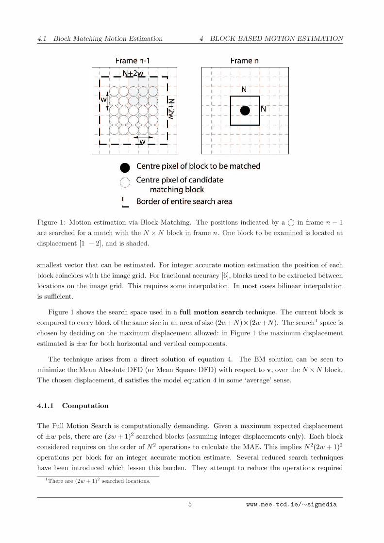
Figure 1: Motion estimation via Block Matching. The positions indicated by a © in frame n − 1are searched for a match with the N ×N block in frame n. One block to be examined is located atdisplacement [1 − 2], and is shaded.

smallest vector that can be estimated. For integer accurate motion estimation the position of eachblock coincides with the image grid. For fractional accuracy [6], blocks need to be extracted betweenlocations on the image grid. This requires some interpolation. In most cases bilinear interpolationis sufficient.

Figure 1 shows the search space used in a full motion search technique. The current block iscompared to every block of the same size in an area of size (2w+N)×(2w+N). The search1 space ischosen by deciding on the maximum displacement allowed: in Figure 1 the maximum displacementestimated is ±w for both horizontal and vertical components.

The technique arises from a direct solution of equation 4. The BM solution can be seen tominimize the Mean Absolute DFD (or Mean Square DFD) with respect to v, over the N ×N block.The chosen displacement, d satisfies the model equation 4 in some ‘average’ sense.

4.1.1 Computation

The Full Motion Search is computationally demanding. Given a maximum expected displacementof ±w pels, there are (2w + 1)2 searched blocks (assuming integer displacements only). Each blockconsidered requires on the order of N2 operations to calculate the MAE. This implies N2(2w + 1)2

operations per block for an integer accurate motion estimate. Several reduced search techniqueshave been introduced which lessen this burden. They attempt to reduce the operations required

1There are (2w + 1)2 searched locations.



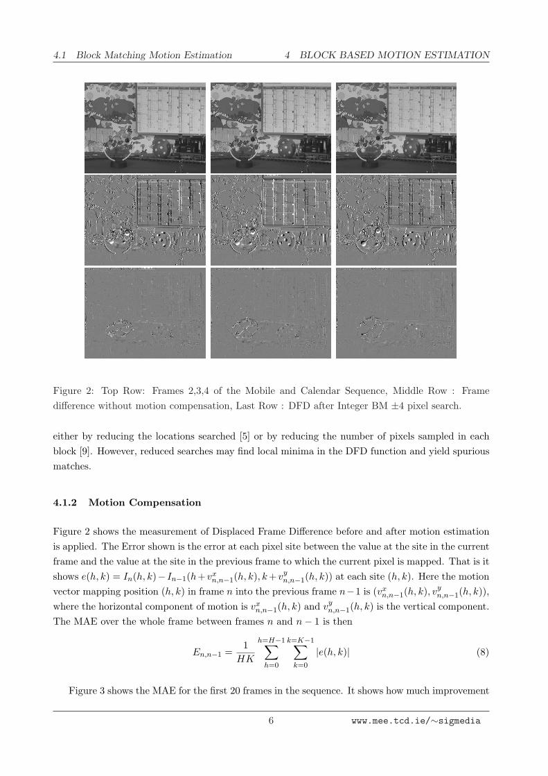
Figure 2: Top Row: Frames 2,3,4 of the Mobile and Calendar Sequence, Middle Row : Framedifference without motion compensation, Last Row : DFD after Integer BM ±4 pixel search.

either by reducing the locations searched [5] or by reducing the number of pixels sampled in eachblock [9]. However, reduced searches may find local minima in the DFD function and yield spuriousmatches.

4.1.2 Motion Compensation

Figure 2 shows the measurement of Displaced Frame Difference before and after motion estimationis applied. The Error shown is the error at each pixel site between the value at the site in the currentframe and the value at the site in the previous frame to which the current pixel is mapped. That is itshows e(h, k) = In(h, k)− In−1(h+vx

n,n−1(h, k), k +vyn,n−1(h, k)) at each site (h, k). Here the motion

vector mapping position (h, k) in frame n into the previous frame n−1 is (vxn,n−1(h, k), vy

n,n−1(h, k)),where the horizontal component of motion is vx

n,n−1(h, k) and vyn,n−1(h, k) is the vertical component.

The MAE over the whole frame between frames n and n− 1 is then

En,n−1 =1

HK

h=H−1∑

h=0

k=K−1∑

k=0

|e(h, k)| (8)

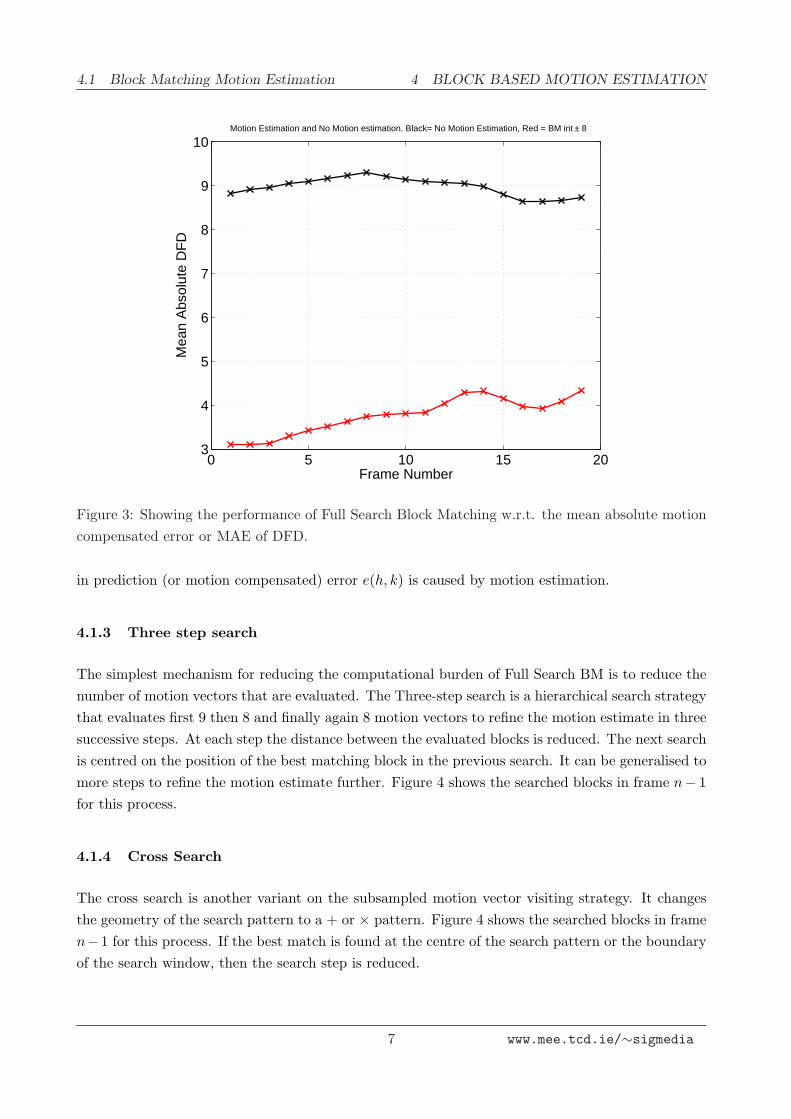
Figure 3 shows the MAE for the first 20 frames in the sequence. It shows how much improvement



0 5 10 15 203

4

5

6

7

8

9

10 Motion Estimation and No Motion estimation. Black= No Motion Estimation, Red = BM int ± 8

Frame Number

Mea

n A

bsol

ute

DF

D

Figure 3: Showing the performance of Full Search Block Matching w.r.t. the mean absolute motioncompensated error or MAE of DFD.

in prediction (or motion compensated) error e(h, k) is caused by motion estimation.

4.1.3 Three step search

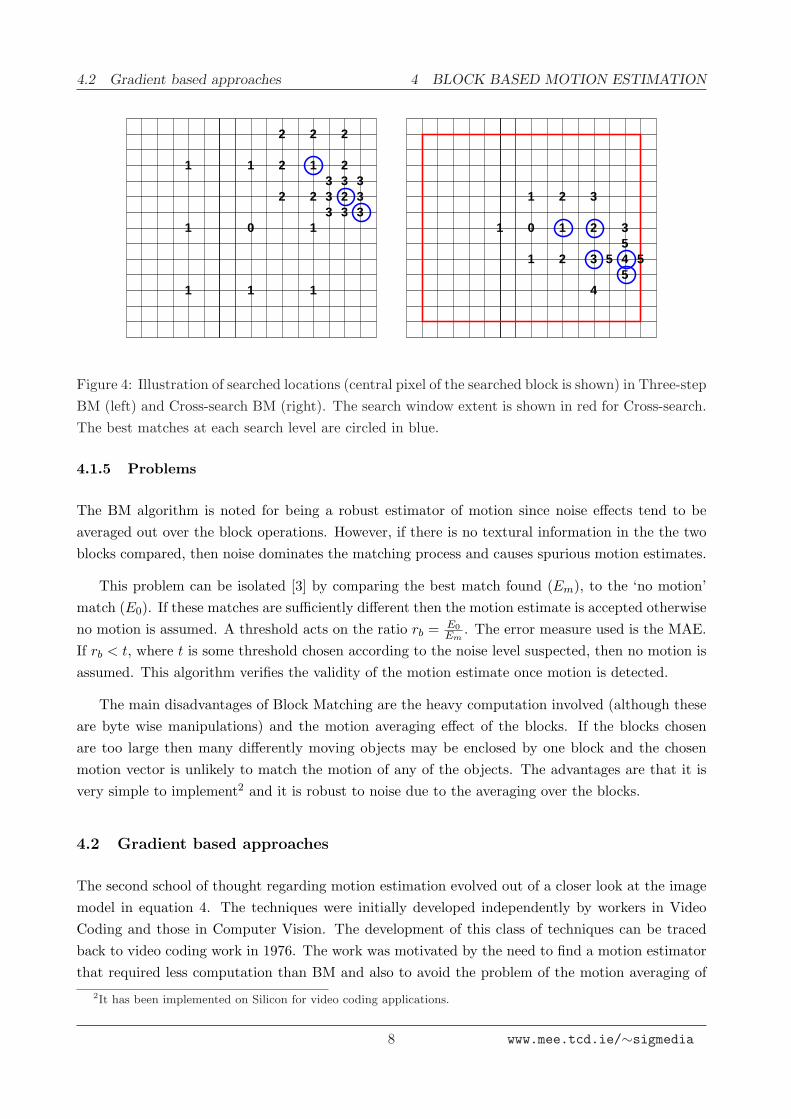
The simplest mechanism for reducing the computational burden of Full Search BM is to reduce thenumber of motion vectors that are evaluated. The Three-step search is a hierarchical search strategythat evaluates first 9 then 8 and finally again 8 motion vectors to refine the motion estimate in threesuccessive steps. At each step the distance between the evaluated blocks is reduced. The next searchis centred on the position of the best matching block in the previous search. It can be generalised tomore steps to refine the motion estimate further. Figure 4 shows the searched blocks in frame n− 1for this process.

4.1.4 Cross Search

The cross search is another variant on the subsampled motion vector visiting strategy. It changesthe geometry of the search pattern to a + or × pattern. Figure 4 shows the searched blocks in framen−1 for this process. If the best match is found at the centre of the search pattern or the boundaryof the search window, then the search step is reduced.


4.2 Gradient based approaches 4 BLOCK BASED MOTION ESTIMATION

3

1

1

1

11

1

1

1

0

2 2

2

222

2

2

3 3 33333

501

1

1

1

2

2

2

3

3

3

4

45

5 5

Figure 4: Illustration of searched locations (central pixel of the searched block is shown) in Three-stepBM (left) and Cross-search BM (right). The search window extent is shown in red for Cross-search.The best matches at each search level are circled in blue.

4.1.5 Problems

The BM algorithm is noted for being a robust estimator of motion since noise effects tend to beaveraged out over the block operations. However, if there is no textural information in the the twoblocks compared, then noise dominates the matching process and causes spurious motion estimates.

This problem can be isolated [3] by comparing the best match found (Em), to the ‘no motion’match (E0). If these matches are sufficiently different then the motion estimate is accepted otherwiseno motion is assumed. A threshold acts on the ratio rb = E0

Em. The error measure used is the MAE.

If rb < t, where t is some threshold chosen according to the noise level suspected, then no motion isassumed. This algorithm verifies the validity of the motion estimate once motion is detected.

The main disadvantages of Block Matching are the heavy computation involved (although theseare byte wise manipulations) and the motion averaging effect of the blocks. If the blocks chosenare too large then many differently moving objects may be enclosed by one block and the chosenmotion vector is unlikely to match the motion of any of the objects. The advantages are that it isvery simple to implement2 and it is robust to noise due to the averaging over the blocks.

4.2 Gradient based approaches

The second school of thought regarding motion estimation evolved out of a closer look at the imagemodel in equation 4. The techniques were initially developed independently by workers in VideoCoding and those in Computer Vision. The development of this class of techniques can be tracedback to video coding work in 1976. The work was motivated by the need to find a motion estimatorthat required less computation than BM and also to avoid the problem of the motion averaging of

2It has been implemented on Silicon for video coding applications.



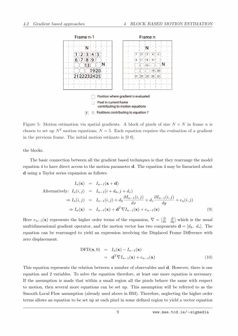
Figure 5: Motion estimation via spatial gradients. A block of pixels of size N × N in frame n ischosen to set up N2 motion equations; N = 5. Each equation requires the evaluation of a gradientin the previous frame. The initial motion estimate is [0 0].

the blocks.

The basic connection between all the gradient based techniques is that they rearrange the modelequation 4 to have direct access to the motion parameter d. The equation 4 may be linearized aboutd using a Taylor series expansion as follows:

In(x) = In−1(x + d)

Alternatively: In(i, j) = In−1(i + dh, j + dv)

⇒ In(i, j) = In−1(i, j) + dh∂In−1(i, j)

dx+ dv

∂In−1(i, j)dy

+ en(i, j)

⇒ In(x) = In−1(x) + dT∇In−1(x) + en−1(x) (9)

Here en−1(x) represents the higher order terms of the expansion, ∇ = [ ∂dx

∂dy ] which is the usual

multidimensional gradient operator, and the motion vector has two components d = [dh, dv]. Theequation can be rearranged to yield an expression involving the Displaced Frame Difference withzero displacement.

DFD(x, 0) = In(x)− In−1(x)

= dT∇In−1(x) + en−1(x) (10)

This equation represents the relation between a number of observables and d. However, there is oneequation and 2 variables. To solve the equation therefore, at least one more equation is necessary.If the assumption is made that within a small region all the pixels behave the same with respectto motion, then several more equations can be set up. This assumption will be referred to as theSmooth Local Flow assumption (already used above in BM). Therefore, neglecting the higher orderterms allows an equation to be set up at each pixel in some defined region to yield a vector equation



as below. The situation is illustrated in Figure 5.

z0 = Gd (11)

where z0 =

DFD(x1, 0)DFD(x2, 0)...DFD(xN2 , 0)

and G =

∂∂xIn−1(x1) ∂

∂y In−1(x1)∂∂xIn−1(x2) ∂

∂y In−1(x2)...

...∂∂xIn−1(xN2) ∂

∂y In−1(xN2)

In Figure 5, the set of N2 equations is set up using the block indicated. The vectors are thereforegenerated by assembling the row–wise observations into columns. The gradient measurements aremade using a simple difference technique, for example the horizontal gradient at pixel 2 in Figure 5is I(3)−I(1)

2 . This is admittedly a noisy process and a more robust class of gradient estimationtechniques, using curve fitting can be used. These are not discussed here.

A solution for d can then be generated using a pseudoinverse approach as follows.

z0 = Gd

⇒ GTz0 = GTGd

⇒ d = [GTG]−1GTz0 (12)

This solution yields d in one step by using gradient measurements in some region as in Figure 5.It is one of the early solutions proposed by Cafforio et al, Netravali et al, Martinez [7] and others.The important drawback with this approach, recognized in [8], is that the Taylor series expansion isonly valid over very small distances. To overcome this problem, a recursive solution was introducedcalled the pel–recursive approach. This new solution refines an initial estimate for d until no furtherreduction in DFD is observed.

4.2.1 Pel-recursive Motion Estimation

Rather than expand the model equation about x, the image function is linearized about a currentguess for d, say di. The idea is to generate an update, u for the current estimate that will eventuallyforce the estimation process to converge on the correct displacement. The update is defined suchthat d = di + ui. The update is intended to be a small one to maintain the validity of the Taylorseries expansion. Therefore, equation 9 becomes

ui = d− di

⇒ In(x) = In−1(x + di + ui)



Expanding about ui then yields

In(x) = In−1(x + di) + uTi ∇In−1(x + di) + en−1(x + di) (13)

The solution may then continue as before. In this case, the only difference between the solution inequation 12 and this one is that the displacement estimate in 12 is used to recursively update thecurrent estimate. The process then continues again.

The algorithm can be summarised in effect as

1. Establish an initial estimate for motion di

2. Using this estimate, fetch the motion compensated block in the previous frame that correspondsto the one being processed in the current frame.

3. Evaluate G, z for these blocks

4. Solve for the update motion estimate, u = [GTG]−1GTz

5. Update the current estimate to yield a new estimate di+1 = di + u

4.2.2 A Wiener estimate

A Wiener solution for the displacement (first introduced in [1]) is more robust to noise. It handlesthe higher order terms more effectively by considering their effect on the solution to be the same asGaussian white noise. The new vector equation to be solved becomes

zi = Gui + e (14)

e(x + di) represents the higher order terms which are considered to be Gaussian white noise ofvariance σ2

ee. Note that the matrices G, zi, now consist of terms similar to those defined earlier inequation 11, but the arguments are offset by the current estimated displacement, di. Compare thisto z0 = Gd which is used in standard gradient based motion estimation.

The Wiener solution chooses the update ui = Lzi which minimizes the expected value of thesquared error between the true update ui and the estimate ui. The objective function is therefore,

E[(ui − ui)T (ui − ui)] (15)

Minimizing this function with respect to L yields the following solution for ui.

ui = [GTG + µI]−1GTz (16)

µ =σ2

ee

σ2uu

Here, σ2uu is the variance of the estimate for ui, provided that both components of the motion have

the same variance. Also, note the use of µ as a regularizing term in the required matrix inverse. The



success of the method lies in treating the observables z,G, e as random variables. The estimatorwill be referred to as the Wiener based motion estimator (WBME) in future references.

After the update is estimated, di is refined to yield the displacement that is used in the nextiteration, di+1 = di + ui, and the process continues again.

4.2.3 Interpolation and convergence

During the iterative process of gradient based motion estimation, the observables may have to beevaluated at fractional displacements. This is because the solution of the equations above do nottypically result in integer accurate motion estimates. Usually bilinear interpolation is employed tokeep computation at a minimum.

Iteration is terminated when the algorithm converges. This is usually detected by thresholdingthe size of the update vector and the size of the current Mean Square Error. When either of thesetwo quantities are below their respective thresholds, convergence is assumed.

4.2.4 Advantages and Disadvantages

The main advantage of the Wiener based pel–recursive estimator is that it requires much less com-putation than the Block Matching algorithm. It is also capable of resolving both fractional andinteger displacements without changing the number of operations involved. Because the computa-tional complexity is so low, many in the Video Coding field have used the technique to estimate amotion vector at each pixel. This is done so that there is less chance of the ‘motion averaging’ effectof blockwise manipulations. The approach is of limited use because some finite support region mustalways be employed to set up the necessary equations. Depending on the size of that region, errorsare likely.

The most important disadvantage of the estimator is that even as an iterative process, it cannotestimate large displacements because of the limited effectiveness of the first order Taylor seriesexpansion. This is in contrast to BM which is only limited by the defined search space. This is avery large problem with gradient based motion estimators.

Finally, all gradient based motion estimators fail when the conditioning of the matrix productGTG is poor. This happens when the searched block has no texture, or when there is a single edgethough the block. It is possible to use the eigenvalues and eigenvectors of this matrix to identifywhen these problems occur. This is a more advanced topic.


5 AMBIGUITY IN MOTION ESTIMATION

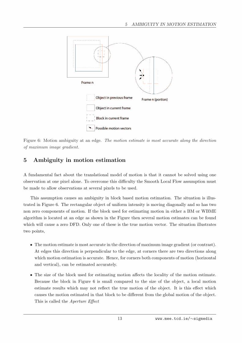
Figure 6: Motion ambiguity at an edge. The motion estimate is most accurate along the directionof maximum image gradient.

5 Ambiguity in motion estimation

A fundamental fact about the translational model of motion is that it cannot be solved using oneobservation at one pixel alone. To overcome this difficulty the Smooth Local Flow assumption mustbe made to allow observations at several pixels to be used.

This assumption causes an ambiguity in block based motion estimation. The situation is illus-trated in Figure 6. The rectangular object of uniform intensity is moving diagonally and so has twonon zero components of motion. If the block used for estimating motion in either a BM or WBMEalgorithm is located at an edge as shown in the Figure then several motion estimates can be foundwhich will cause a zero DFD. Only one of these is the true motion vector. The situation illustratestwo points,

• The motion estimate is most accurate in the direction of maximum image gradient (or contrast).At edges this direction is perpendicular to the edge, at corners there are two directions alongwhich motion estimation is accurate. Hence, for corners both components of motion (horizontaland vertical), can be estimated accurately.

• The size of the block used for estimating motion affects the locality of the motion estimate.Because the block in Figure 6 is small compared to the size of the object, a local motionestimate results which may not reflect the true motion of the object. It is this effect whichcauses the motion estimated in that block to be different from the global motion of the object.This is called the Aperture Effect


7 OPTIC FLOW

If the block used for motion estimation is located in the centre of the moving object in Figure 6,then it is likely that neither estimator will estimate any motion at all. There will be zero error forzero displacement and so the motion detector will not flag motion. Even if motion estimation wereto be engaged then the zero or near zero DFD coupled with the zero gradient in the previous framewill bias the result toward a zero motion vector.

6 Adaptive Gradient Based Motion Estimation

Most of the problems with the block based gradient estimators like WBME occur when the gradientmatrix is ill-conditioned. This can be dealt with by adapting µ in the WBME to the ill–conditioningof Mg = [GTG] during the pel–recursive process. One possibility is shown below

d = [GTG + µI]−1GT z (17)

where µ = |z|λmax

λmin

where λ are the eigen values of the 2 × 2 matrix Mg. As the required inverse solution becomesill–conditioned (measured as a ratio of eigenvalues), µ increases, thus increasing the damping in thesystem. The additional multiplying factor of |z| helps to further stabilize the situation by relaxingthe damping when the error is small and the motion estimate is close to convergence.

A full SVD decomposition of Mg leads to the best adaptive scheme. Since Mg is just a 2 × 2matrix, the computational load of this step is very small.

7 Optic Flow

Given I(x, y, t) is the intensity of a pixel at (x, y) at time t, assuming the intensity is constant alonga motion trajectory we have

dI(x(t), y(t), t)dt

= 0 (18)

Using the chain rule for differentiation this can be expressed as

∂I(x, y, t)dx

∂x

dt+

∂I(x, y, t)dy

∂y

dt+

∂I(x, y, t)dt

= 0 (19)

The partial derivatives ∂xdt , ∂y

dt are the components of horizontal and vertical velocities at site (x, y)respectively. This equation is known as the Optical Flow Equation and can be written as

uhgh(x, t) + uvgv(x, t) +∂I(x, t)

dt= 0 (20)

where uh, uv are the horizontal and vertical components of motion, gh, gv are horizontal and verticalspatial gradients, and ∂I(x,t)

dt is the instantaneous DFD at pixel site x. This equation can also bederived from the Taylor Series expansion in equation 10 assuming the error in the expansion is zero.


8 MULTIRESOLUTION MOTION ESTIMATION

The Optic Flow constraint is valid only for small uh, vh and has been used to estimate motion on apixel basis. To do so, it is necessary to incorporate a constraint on the motion field as well. Assumingthat objects tend to be rigid, then the motion field in a local region should be smooth. These twoconstraints were used by Horn and Schunck to estimate motion using an iterative algorithm.

Define the horizontal and vertical components of motion at a site d(x) = [d1(x), d2(x)]. Thenthe task is to minimise the spatial variation in the motion field Ds(x)

Ds(x) =(

∂d1

dx

)2

+(

∂d1

dy

)2

+(

∂d2

dx

)2

+(

∂d2

dy

)2

(21)

with the constraint that the Optical Flow equation is satisfied.

It is possible to further adapt this method by altering the spatial motion smoothness measureDs above. Since edges in an image usually coincide with object edges, and since different objectscan move in different directions, motion should not be smooth across an object edge, hence shouldnot be the same across an image edge. Thus the smoothness constraint above can be relaxed acrossimage edges. This leads to a much improved motion estimation process.

8 Multiresolution Motion Estimation

Throughout the discussion so far it has been noted that gradient based techniques can only effectivelyestimate small displacements. A correspondence technique, such as BM, is only limited in thisrespect by the extent of the search space used. However, increasing the search space to deal with alarge displacement, increases the computational requirement. Considering that motion pictures caninvolve displacements in excess of 10 pixels per frame, increasing the search space of BM to dealwith this motion results in a huge increase in computation.

It has been widely accepted that the multiresolution schemes provide the most practical way ofdealing with this problem effectively. The idea of a multiresolution representation was presented earlyon for use in Image Coding by Burt and Adelson [4]. The technique can reduce the computationalrequirement to estimate a particular displacement in the case of BM [2]. In the case of gradientbased techniques, the scheme can make the problem better conditioned and increase convergencerates.

The concept is simple. Create a series of images at successively coarser resolution, then beginmotion estimation at the coarsest scale. The motion estimates are refined at each successively higherresolution level.

8.1 Low Pass Pyramid

The multiresolution scheme begins by building successively smaller versions of the images in terms ofspatial extent, while still maintaining useful image information in each version. The original images


8.2 Creating the pyramid 8 MULTIRESOLUTION MOTION ESTIMATION

are low pass filtered and subsampled until the displacements measured in the subsampled framesare small enough to allow reasonably accurate pel–recursive, or BM motion estimation with a smallsearch space.

The motion vectors found at the lower resolutions are then projected onto the higher resolutionswhere the motion estimation process is allowed to continue. Successive projections of the estimatedmotion field eventually leads to an initial motion field at the highest resolution and then it ispresumed that only a few iterations will be needed for a pel–recursive algorithm to converge. In thecase of BM the search space at each level can be drastically reduced, because a small displacementat the higher levels represents a large displacement at the original level. It is typical to subsampleby a factor of 2 so that if the original level is of resolution H × V then level l of N levels has a sizeH2l × V

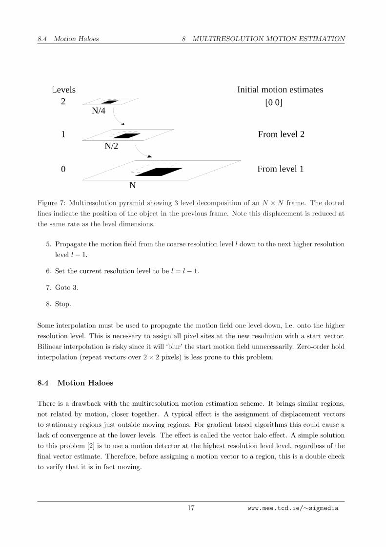
2l . Motion of magnitude k pixels at level 0 (the original resolution level), is then reduced tok × 2−(N−1) at level N − 1. Figure 7 illustrates the pyramidal representation.

The underlying motivation for a multiresolution approach here is to create a representation ofthe original image in which the motion is small enough to allow a motion estimation algorithm toterminate successfully. To this end the basic character of the image at the varying scales must bemaintained. This is necessary to ensure that the motion fields estimated at the lower resolutionsbear some resemblance to the actual motion field at the original resolution.

8.2 Creating the pyramid

A Gaussian shaped low pass filter is typically used to create the pyramid and also slightly blurthe image at each scale. This latter point is useful in that it artificially increases the proportionof the first order term in the Taylor series expansion of the image function, thus stabilizing theiterative process. Further, the filter is non directional and so does not favour motion estimation inany direction.

8.3 Algorithm

The multigrid motion estimation algorithm is enumerated below

1. Generate L levels of the multiresolution pyramid, such that level l = 0 is the original resolutionimage, and level l = L− 1 is the image with the smallest resolution.

2. Set the initial level to be the level with the most coarse resolution, level l = L − 1. Set theinitial field at this level to be a set of zero vectors.

3. Generate an estimate of the motion field at the resolution level l using the current startingfield.

4. If l = 0 then goto 8.


8.4 Motion Haloes 8 MULTIRESOLUTION MOTION ESTIMATION

N

N/2

N/4

Levels2

1

0

Initial motion estimates

[0 0]

From level 2

From level 1

Figure 7: Multiresolution pyramid showing 3 level decomposition of an N × N frame. The dottedlines indicate the position of the object in the previous frame. Note this displacement is reduced atthe same rate as the level dimensions.

5. Propagate the motion field from the coarse resolution level l down to the next higher resolutionlevel l − 1.

6. Set the current resolution level to be l = l − 1.

7. Goto 3.

8. Stop.

Some interpolation must be used to propagate the motion field one level down, i.e. onto the higherresolution level. This is necessary to assign all pixel sites at the new resolution with a start vector.Bilinear interpolation is risky since it will ‘blur’ the start motion field unnecessarily. Zero-order holdinterpolation (repeat vectors over 2× 2 pixels) is less prone to this problem.

8.4 Motion Haloes

There is a drawback with the multiresolution motion estimation scheme. It brings similar regions,not related by motion, closer together. A typical effect is the assignment of displacement vectorsto stationary regions just outside moving regions. For gradient based algorithms this could cause alack of convergence at the lower levels. The effect is called the vector halo effect. A simple solutionto this problem [2] is to use a motion detector at the highest resolution level level, regardless of thefinal vector estimate. Therefore, before assigning a motion vector to a region, this is a double checkto verify that it is in fact moving.


REFERENCES

9 Summary

Motion estimation is key for the processing of digital video. There are two main classes of motionestimator, those based on Block Matching and those based on gradient analysis of some kind. All themotion estimators can estimate motion pixel by pixel or on a block basis, however it is understoodthat the motion equation cannot be solved at a single pixel site alone.

The two main problems with block based motion are the aperture problem and the motionambiguity at a strong image edge. Motion estimation is therefore most accurate at corners in theimage. The drawbacks of gradient based motion are typically that motion cannot be estimatedwhere there is no image gradient, and the motion must be small. However gradient based estimatorsare generally of lower computational load than BM estimators, and are more accurate.

Many of the problems with BM and computational load can be overcome with a multiresolutionscheme for motion estimation. Similarly the difficulties with the small motion assumption in gradientbased motion estimation can be overcome with multiresolution schemes.

The book Digital Video Processing, Murat Tekalp, Prentice Hall, ISBN 0-13-190075-7 has excel-lent coverage of motion estimation techniques. Lim covers a practical range of techniques in pages497-506.

References

[1] J. Biemond, L. Looijenga, D. E. Boekee, and R.H.J.M. Plompen. A pel–recursive Wiener baseddisplacement estimation algorithm. Signal Processing, 13:399–412, 1987.

[2] M. Bierling. Displacement estimation by heirarchical block matching. In SPIE VCIP, pages942–951, 1988.

[3] J. Boyce. Noise reduction of image sequences using adaptive motion compensated frame averag-ing. In IEEE ICASSP, volume 3, pages 461–464, 1992.

[4] P. Burt and E. Adelson. The Laplacian pyramid as a compact image code. IEEE transactionson Communications, 31:532–540, April 1983.

[5] M. Ghanbari. The cross–search algorithm for motion estimation. IEEE Transactions on Com-munications, 38:950–953, July 1990.

[6] B. Girod. Motion–compensating prediction with fractional–pel accuracy. IEEE Transactions onCommunications, Accepted March 1991.

[7] D. M. Martinez. Model–based motion estimation and its application to restoration and interpo-lation of motion pictures. PhD thesis, Massachusetts Institute of Technology, 1986.


REFERENCES REFERENCES

[8] A. Netravali and J. Robbins. Motion–compensated television coding: Part 1. The Bell SystemTechnical Journal, 58:631–670, March 1978.

[9] A. Zaccarin and B. Liu. Fast algorithms for block motion estimation. In IEEE ICASSP, volume 3,pages 449–452, 1992.


Documents

Motion Estimation Image and Video Processing Dr. Anil ...sigmedia/pmwiki/uploads/Teaching.4S1b/handout9_4s1.pdf · Motion Estimation Image and Video Processing Dr. Anil Kokaram [email protected]