Motion of the cello bridgeAilin ZhangJim WoodhouseGeorge StoppaniJW

Citation: J. Acoust. Soc. Am. 140, 2636 (2016); doi: 10.1121/1.4964609View online: http://dx.doi.org/10.1121/1.4964609View Table of Contents: http://asa.scitation.org/toc/jas/140/4Published by the Acoustical Society of America

Articles you may be interested inMechanics of human voice production and controlJ. Acoust. Soc. Am. 140, (2016); 10.1121/1.4964509

Delay-based ordered detection for layered space-time signals of underwater acoustic communicationsJ. Acoust. Soc. Am. 140, (2016); 10.1121/1.4964820

Motion of the cello bridge

Ailin Zhanga)

College of Mathematics and Statistics, Shenzhen University, 3688 Nanhai Avenue Shenzhen, Guangdong,People’s Republic of China

Jim WoodhouseDepartment of Engineering, University of Cambridge, Trumpington Street, Cambridge CB2 1PZ,United Kingdom

George Stoppani6 Needham Avenue, Chorlton-cum-Hardy, Manchester M21 8AA, United Kingdom

(Received 24 May 2016; revised 12 September 2016; accepted 22 September 2016; publishedonline 14 October 2016)

This paper presents an experimental investigation of the motion of the bridge of a cello, in the

frequency range up to 2 kHz. Vibration measurements were carried out on three different cellos,

and the results used to determine the position of the Instantaneous Centre of rotation of the bridge,

treated as a rigid body. The assumption of rigid body rotation is shown to give a good approxima-

tion up to at least 1 kHz. The instantaneous centre moves from the sound-post side of the bridge

at the lowest frequencies towards the bass-bar side at higher frequencies, remaining close to the

surface of the top plate of the instrument. The trajectory as a function of frequency sheds light on

the response of the cello in response to excitation by bowing the different strings. The correlation

between the motion at the four string notches and directly measured transfer functions at these four

notches is examined and verified for some important low-frequency body resonances.VC 2016 Acoustical Society of America. [http://dx.doi.org/10.1121/1.4964609]

[JW] Pages: 2636–2645

I. INTRODUCTION

The bridge on most bowed string instruments is made

from specially selected maple. It is held in place only by the

tension of strings, and plays a critical transfer role between

the vibrating strings and the radiating corpus during sound

production on the instrument. An intelligently cut and well

fitted bridge can have a profound influence on the tonal char-

acteristics of a bowed string instrument, as makers and play-

ers have been aware for centuries.

The bridge has also attracted interest from scientists.

Research up to 1993 has been summarized by Hutchins and

Benade.1 Minnaert and Vlam2 reported the first detailed

investigation into the flexural, torsional, and transverse

vibration of a violin bridge using a specially designed optical

system. The first study on the motion of a cello bridge was

done by Bladier3 in 1960 using a piezoelectric transducer

fastened to the tested bridge. He showed differences between

the motions at the two bridge feet. In 1979, Reinicke4 dis-

played the motion of a violin bridge and a cello bridge using

hologram interferometry, and modelled the motions mathe-

matically. Experiments on the design of the violin bridge

were made by M€uller5 in 1979. He measured the sound pres-

sure with differently designed bridges and discussed the

function of the bridge. Cremer6 described this work in his

remarkable book summarizing knowledge about the violin

family up to 1983.

Rodgers and Masino7 and Kishi and Osanai8 examined

bridge motion under different conditions using finite element

analysis. On a more practical level, Jansson and his co-work-

ers9–11 investigated the effect of bridge modification on the

vibrational behaviour of the instrument. They started with

the influence of wood removal from different areas of the

bridge and then turned their attention to the bridge foot spac-

ing. Trott12 used a shaker and an impedance head to measure

the power input to a violin bridge when excited in various

positions and directions.

The first work that relates directly to the present study

came from Marshall,13 who observed that a violin bridge

shows more motion at the bass foot than at the treble foot up

to 700 Hz. Later modal and acoustical measurements explor-

ing the action of the violin bridge as a filter were carried out

by Bissinger.14 His experimental results also showed a tran-

sition of the predominant motion of the feet of a violin

bridge from the bass side to the treble side, confirming and

extending the findings of Marshall.

This observation links to a familiar claim about the role

of the soundpost in violin-family instruments: the soundpost

produces a constraint near the treble foot of the bridge at low

frequencies, inducing asymmetry in the vibration patterns

and boosting the sound radiation in the monopole-dominated

regime at low frequencies (see, for example, Cremer6). The

effect is sometimes informally described by saying that

the bridge “rocks around the soundpost” at low frequencies.

The transition documented by Marshall and Bissinger may

define the correct sense of “at low frequencies.” Some

authors have taken to referring to this frequency range as the

“transition region,” and a feature commonly seen in violina)Electronic mail: az304@szu.edu.cn

2636 J. Acoust. Soc. Am. 140 (4), October 2016 VC 2016 Acoustical Society of America0001-4966/2016/140(4)/2636/10/$30.00

frequency response has been dubbed the “transition hill”

(see, for example, Gough15). This phenomenon is the main

topic of the present work. Detailed measurements of bridge

motion will be shown, and analyzed in a way that gives a

new perspective on this transition.

The measurements also shed light on another question

of some current interest, relating to possible differences in

coupling to the instrument body of the four separate strings.

The single most common acoustical measurement on violin-

family instruments is an approximation to the driving-point

admittance (or mobility) at the top of the bridge. Most

researchers use some version of a technique originated by

Jansson,16 in which a force is applied to one corner of a

bridge, usually by a miniature impulse hammer, and the

motion is measured at the other corner using a laser vibrome-

ter or miniature accelerometer. For a detailed discussion of

such measurements and their interpretation, see Woodhouse

and Langley.17 It would be very useful to quantify how well

this corner-to-corner measurement in fact represents the

admittance felt by the four individual strings at their respec-

tive bridge notches, in the usual bowing direction tangential

to the bridge top. For a perfect match to all four strings, the

motion of the top part of the bridge would need to follow

around the line of the curved shape of the bridge.

Another way to pose this requirement, familiar to

mechanical engineers (see, for example, Meriam et al.18), is

to say, that the “instantaneous center of rotation” of the top

part of the bridge would need to lie at the geometric center

of the bridge-top curve. This formulation stems from a theo-

rem of kinematics: planar motion of any rigid body, at any

given instant, can be represented completely by rotation at

some angular velocity about a point known as the instanta-

neous center (IC). The suggestion that the bridge “rocks

around the soundpost at low frequencies” is, of course, a

direct claim about the position of the IC. In the context of

small vibration governed by linear theory, it is natural to

examine the motion associated with the separate harmonic

frequencies making up the admittance function, and in those

terms the IC can be expected to move around as a function

of frequency. When its trajectory lies near the geometric

center of the bridge curve, the four strings will “feel” the

body response in a similar way, accurately represented

by the standard measurement. If it lies far from that point,

however, the strings will experience significantly different

responses.

The work reported here will use this paradigm to exam-

ine the motion of a cello bridge in the low- to mid-frequency

range, where its in-plane motion can be expected to be

essentially rigid. The cello bridge, which is very different

from a violin bridge in proportions, has been less empha-

sized in the musical acoustics literature. As well as having

intrinsic interest, its larger size makes the necessary meas-

urements easier. Vibration transfer function measurements at

several points around the bridge and on the top plate near the

bridge feet were carried out on three cellos. The responses at

these points at any given frequency were processed to find

the best-fitted rigid-body motion of the bridge, from which

the IC can be located. This IC position can then be tracked

as a function of frequency, giving an immediate visual test

of how strong a constraint the soundpost offers, and an

impression of how similar or different the body response

will appear to the four strings.

It is perhaps worth stating explicitly what will not be

covered here. Modal analysis of the bridge to show the

deformations at higher frequencies has been well covered in

previous work, and will not be repeated here. The first defor-

mational resonance of the bridge will set the upper limit to

the frequency range of interest here: around and above that

frequency, “hill-like” features in the instrument response are

to be expected, as has been discussed in various earlier liter-

ature (see, for example, Ref. 17). At lower frequencies,

although there will be some discussion of resonances of the

cello body in relation to wolf notes and other playability

issues, detailed modal analysis of the body is not directly rel-

evant to the agenda here. The clear and restricted aim of this

study is to visualise the associated bridge motion in a novel

way via the trajectory of the IC. This will have implications

for the “transition region,” and also for issues of playability

such as the notorious cello wolf note.19 Playability differ-

ences between the strings of the instrument will be dis-

cussed, and possible limitations of the conventional single

measurement of bridge admittance.

II. EXPERIMENTS

A. Instruments to be tested

Systematic experiments were conducted on three differ-

ent cellos, which were fitted with different shapes of bridges.

For convenience, these three cellos are labelled Cello 1,

Cello 2, and Cello 3 in the remainder of this paper. The first

cello was a student instrument of moderate quality, made

by an unknown maker, fitted with a Belgian design bridge.

The upper body shape and longer legs of Belgian bridges are

generally thought to give a brighter and louder sound. The

width between the outside foot-edges is 90 mm, and the

height from the middle point of its bass bar side foot to its

top is 95 mm. The second cello is one made some forty years

ago by the second author, fitted with a French design bridge.

The length of legs of this bridge accounts for approximately

half its height, shorter than those of the Belgian counterpart.

The width between its outside foot-edges is 92 mm and the

height from the middle point of its bass bar side foot to its

top is 91 mm. In general, French bridges appear lower and

wider than their Belgian counterparts, and are often said to

be somewhat darker sounding. The third cello is a new

instrument made by the third author. It has a typical Belgian

design bridge, which shares the same outline dimensions as

the first one.

B. Measurement procedure

To resemble the holding manner of a player, the cellos

were held for testing within a steel support frame, steadied

by soft foam pieces in a similar way to the player’s knees.

The cello endpin was located in a hole at the base of the rig,

and the neck was fastened by a cable tie to a shaped and

rubber-lined block behind the neck in first position. This rig

is described in more detail in an earlier paper.20 All

J. Acoust. Soc. Am. 140 (4), October 2016 Zhang et al. 2637

experiments reported here were carried out with the cello

strings correctly tuned and thoroughly damped, and all took

place in the same laboratory acoustic environment.

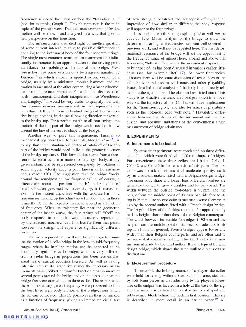
Figure 1 shows the positions of a set of test points on a

cello bridge, and the directions of force application at these

points in order to measure transfer functions. The C-string

corner of the cello bridge is denoted as point 1. Points 1–5

are located on the edge of the cello bridge. Points 6 and 7

cannot be excited directly, but the results are deduced by

averaging measurements made on the top plate near the feet,

symmetrically placed in front and behind the two positions.

Points 8–11 denote the positions of the string notches under

the C, G, D, and A strings, respectively. The geometric center

of the bridge-top curve is marked by a cross-in-circle symbol.

The motion was measured at the C string corner by a

small accelerometer (DJB M2222C) glued to the bridge. It

was orientated so that its center line was parallel to the usual

bowing direction of the cello C string. The accelerometer

mass (including some allowance for its cable) is around

0.8 g, compared with a typical mass of a cello bridge around

19 g. A miniature force hammer (PCB 086D80) held in a

pendulum fixture was used to provide a reliably positioned

force pulse to each point of interest on the cello bridge or top

plate. The set of points shown in Fig. 1 were hit by the ham-

mer in turn. All the hammer impacts were applied in the

plane of the bridge or parallel to it. Forces labelled as F1 and

F3 were applied to points 1 and 3 on the bridge along the

bowing direction of the nearest strings. Impulses labelled as

F2, F4, and F5 were applied to Points 2, 4, and 5 on the sides

of the bridge perpendicular to the surface. Impact forces on

the body to deduce points 6 and 7 were perpendicular to the

top plate. The input and output signals, after buffering with

suitable charge amplifiers, were processed by data logging

software to yield the transfer functions associated with the

seven points. These will be used for calculating the planar

motion of the cello bridge in Sec. III: The measurements

will be interpreted using the familiar reciprocal theorem of

linear vibration, as if they were the motion at the test points

in response to force applied at the bridge corner.

The bridge of cello 1, in addition to the accelerometer,

was fitted with four piezoelectric force sensors to record the

transverse force exerted by the vibrating strings, as described

in earlier work.20 These additional sensors, with their

attached cables, add mass and damping to the bridge and

thus modify the response somewhat, but were necessary to

obtain the vibration response associated with excitation at

the four separate string notches as described earlier20 and

discussed further in Sec. IV.

III. CALCULATION OF BRIDGE MOTION

In the lower frequency range, the bridge is expected to

move approximately as a rigid body with little deformation. A

simple least-squares calculation can be used to determine that

rigid motion from the set of measurements described in Sec.

II B. The position of the IC can then be deduced. To describe

the bridge motion, first choose a reference point O and define

Cartesian axes X, Y at this point as shown in Fig. 2. Any rigid

motion of the bridge in this plane can now be described by a

linear velocity at O with components (U, V), together with an

angular velocity X about the axis through O perpendicular to

the plane. At a particular measurement point on the bridge with

position vector ðxj; yjÞ relative to O, the velocity vector is then

uj ¼ ðU � Xyj;V þ XxjÞ; (1)

where j ¼ 1; 2; :::; 7:The measured velocity at the test points (obtained by

integrating the accelerometer signal) will be the component

of this velocity in a particular direction determined by the

orientation of the hammer impact. Denoting the unit vector

in that direction by

nj ¼ ðcos uj; sin ujÞ; (2)

the measured velocity associated with the rigid bridge

motion would be

tj ¼ uj � nj ¼ ðU � XyjÞ cos uj þ ðV þ XxjÞ sin uj: (3)

The task now is to best-fit a rigid bridge motion to the set of

measurements, to determine U, V, and X. A natural approach

is to seek to minimise the error measure

q ¼X

j

jmj � tjj2; (4)

where the measured velocities are denoted mj. A standard

least-squares procedure leads to a set of linear equations for

the three unknowns. The position of the IC can then easily

FIG. 1. (Color online) Positions and directions of applied forcing at points

around a cello bridge (points 1–7), together with the positions of the four

string notches (points 8–11). Cross-in-circle symbol: the geometric center of

the bridge-top curve.

2638 J. Acoust. Soc. Am. 140 (4), October 2016 Zhang et al.

be found. This point is defined by the fact that it has no lin-

ear velocity, so from Eq. (1) the coordinates of the IC rela-

tive to O are given by

Xic ¼ �V=X;

Yic ¼ U=X: (5)

However, there is a complicating factor to be consid-

ered. The measured values will be complex numbers, reflect-

ing the fact that at any given frequency there may be a phase

difference between the force and the velocity. In conse-

quence the fitted U, V, and X will be complex, and the coor-

dinates Xic and Yic are thus also complex. To see what this

means for the trajectory of the IC during a cycle of the vibra-

tion (known as the “centrode”18), it is convenient to write

explicitly

U ¼ U0 cosðxtþ n1Þ;V ¼ V0 cosðxtþ n2Þ;X ¼ X0 cosðxtþ n3Þ: (6)

Without loss of generality, define the instant t¼ 0 so that

n3 ¼ 0. Then

Xic ¼V0 cos xtþ n2ð Þ

X0 cos xt¼ � V0

X0

cos n2 � sin n2 tan xtð Þ;

Yic ¼U0 cos xtþ n1ð Þ

X0 cos xt¼ U0

X0

cos n1 � sin n1 tan xtð Þ: (7)

The interpretation of these equations is that during one cycle

of oscillation the IC moves along a straight line, with dis-

tance along this line parameterised by tan xt. This motion

involves travelling to infinity and then back from the

opposite direction. This apparently rather drastic and non-

physical behaviour has a simple interpretation: if the rota-

tional component of motion is not in phase with the linear

motion, there will be an instant when there is no rotation but

non-zero linear velocity, and this requires the center of

rotation to be “at infinity” at that instant. However, for the

practical cases to be shown shortly it is invariably true that

the vast majority of the time is spent near the point where

the tangent function is zero, and discussions will focus on

the position of that point: the movement “to infinity” can be

ignored for the purposes of visualizing the main motion at

the string notches.

IV. EXPERIMENTAL RESULTS

A. Bridge motion

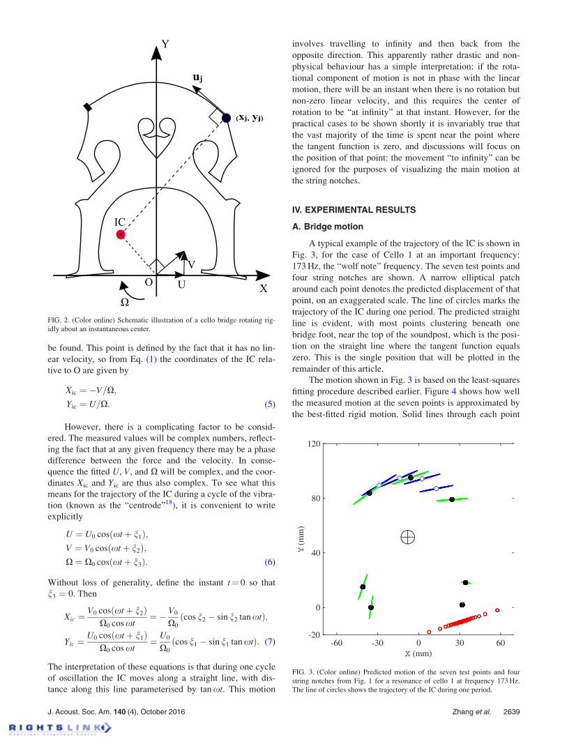
A typical example of the trajectory of the IC is shown in

Fig. 3, for the case of Cello 1 at an important frequency:

173 Hz, the “wolf note” frequency. The seven test points and

four string notches are shown. A narrow elliptical patch

around each point denotes the predicted displacement of that

point, on an exaggerated scale. The line of circles marks the

trajectory of the IC during one period. The predicted straight

line is evident, with most points clustering beneath one

bridge foot, near the top of the soundpost, which is the posi-

tion on the straight line where the tangent function equals

zero. This is the single position that will be plotted in the

remainder of this article.

The motion shown in Fig. 3 is based on the least-squares

fitting procedure described earlier. Figure 4 shows how well

the measured motion at the seven points is approximated by

the best-fitted rigid motion. Solid lines through each point

FIG. 2. (Color online) Schematic illustration of a cello bridge rotating rig-

idly about an instantaneous center.

FIG. 3. (Color online) Predicted motion of the seven test points and four

string notches from Fig. 1 for a resonance of cello 1 at frequency 173 Hz.

The line of circles shows the trajectory of the IC during one period.

J. Acoust. Soc. Am. 140 (4), October 2016 Zhang et al. 2639

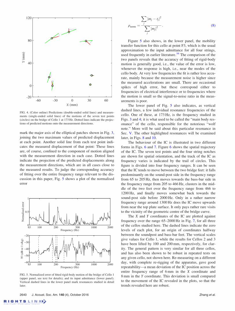
mark the major axis of the elliptical patches shown in Fig. 3,

joining the two maximum values of predicted displacement

at each point. Another solid line from each test point indi-

cates the measured displacement of that point: These lines

are, of course, confined to the component of motion aligned

with the measurement direction in each case. Dotted lines

indicate the projection of the predicted displacements along

the measurement directions, which are in all cases close to

the measured results. To judge the corresponding accuracy

of fitting over the entire frequency range relevant to the dis-

cussion in this paper, Fig. 5 shows a plot of the normalised

error

qnorm ¼

X

j

jmj � tjj2

X

j

jmjj2: (8)

Figure 5 also shows, in the lower panel, the mobility

transfer function for this cello at point F3, which is the usual

approximation to the input admittance for all four strings,

used frequently in earlier literature.16 The comparison of the

two panels reveals that the accuracy of fitting of rigid-body

motion is generally good, i.e., the value of the error is low,

whenever the response is high, i.e., near the modes of the

cello body. At very low frequencies the fit is rather less accu-

rate, mainly because the measurement noise is higher since

the measured accelerations are small. There are occasional

spikes of high error, but these correspond either to

frequencies of electrical interference or to frequencies where

the motion is small so the signal-to-noise ratio in the meas-

urements is poor.

The lower panel of Fig. 5 also indicates, as vertical

dashed lines, a few individual resonance frequencies of the

cello. One of these, at 173 Hz, is the frequency studied in

Figs. 3 and 4; it is what used to be called the “main body res-

onance” of the cello, responsible for the notorious “wolf

note.” More will be said about this particular resonance in

Sec. V. The other highlighted resonances will be examined

later, in Figs. 8 and 10.

The behaviour of the IC is illustrated in two different

forms in Figs. 6 and 7. Figure 6 shows the spatial trajectory

of the IC. The seven test points and the four string notches

are shown for spatial orientation, and the track of the IC as

frequency varies is indicated by the trail of circles. This

figure is divided into four frequency ranges. It can be seen

that the IC tends to move between the two bridge feet: it falls

predominantly on the sound-post side in the frequency range

from 65 to 205 Hz, then moves towards the bass-bar side in

the frequency range from 205 to 466 Hz, clusters in the mid-

dle of the two feet over the frequency range from 466 to

1200 Hz, and finally moves somewhat back towards the

sound-post side before 2000 Hz. Only in a rather narrow

frequency range around 1300 Hz does the IC move upwards

from near the top plate surface. It only pays rather rare visits

to the vicinity of the geometric centre of the bridge curve.

The X and Y coordinates of the IC are plotted against

frequency over the range 65–2000 Hz in Fig. 7, for all three

of the cellos studied here. The dashed lines indicate the zero

levels of each plot, for an origin of coordinates halfway

between the soundpost and bass-bar feet. The vertical scales

give values for Cello 1, while the results for Cellos 2 and 3

have been lifted by 100 and 200 mm, respectively, for clar-

ity. The general pattern is very similar for all three cellos,

and has also been shown to be robust in repeated tests on

any given cello, not shown here. Re-measuring on a different

day, with complete re-rigging of the apparatus, gave good

repeatability—a mean deviation of the IC position across the

entire frequency range of 6 mm in the X coordinate and

8 mm in the Y coordinate. This deviation is small compared

to the movement of the IC revealed in the plots, so that the

trends revealed here are robust.

FIG. 4. (Color online) Predictions (double-ended solid lines) and measure-

ments (single-ended solid lines) of the motions of the seven test points

(circles) on the bridge of Cello 1 at 173 Hz. Dotted lines indicate the projec-

tions of predicted motions onto the measurement directions.

FIG. 5. Normalized error of fitted rigid-body motion of the bridge of Cello 1

(upper panel, see text for details); and its input admittance (lower panel).

Vertical dashed lines in the lower panel mark resonances studied in detail

later.

2640 J. Acoust. Soc. Am. 140 (4), October 2016 Zhang et al.

Up to about 180 Hz, the IC stays close to the top of the

soundpost. In the intermediate range from there up to about

700 Hz it tends to move back and forth between the bridge

feet, always close to the surface of the cello top plate. The

detailed movements are different for each cello because the

well-separated resonances in this frequency range are

different.

At higher frequencies still, the X position moves around

in the vicinity of the mid-point between the bridge feet, but

the Y position does something more interesting. For all three

cellos a conspicuous feature appears in the range 1–1.5 kHz

showing movement first down into the cello body and then

jumping upwards before settling back towards the level of

the bridge base. Digging further into the details of the meas-

urements (not reproduced here), this feature turns out to be

associated with the first resonance of the cello bridge: as

shown by Reinicke4 this involves lateral motion of the

bridge top while the legs “sway” in shear. Reinicke shows

this resonance occurring around 1 kHz for his particular cello

bridge, with its feet rigidly clamped. The in situ bridge reso-

nance for Cello 1 is found to occur at about 1200 Hz, and

those for Cellos 2 and 3 at about 1500 and 1350 Hz, respec-

tively. These frequencies match the visible features in the

FIG. 6. (Color online) Trajectories of

the IC of the bridge of Cello 1 over

four frequency ranges: (a) 65–205 Hz;

(b) 205–466 Hz; (c) 466–1200 Hz; (d)

1200–2000 Hz. Circles show the posi-

tions of the test points and string

notches, cross-in-circle symbol shows

the geometric center of the bridge-top

curve.

FIG. 7. (Color online) X and Y coordinates of the IC of the bridge of Cello 1

(lower line, data as in Fig. 6), Cello 2 (middle line), and Cello 3 (upper line)

over the frequency range 65–2000 Hz. The data for Cello 3 has higher mea-

surement noise at low frequencies. The plots are separated by 100 mm inter-

vals for clarity.

J. Acoust. Soc. Am. 140 (4), October 2016 Zhang et al. 2641

fitted trajectories of the ICs shown in Figs. 6 and 7. Possibly

the frequency is lower for cello 1 than for the others because

of the extra mass of the force sensors built in to its bridge, as

noted earlier. This bridge resonance sets a cutoff frequency

beyond which the analysis and discussion in this paper is no

longer appropriate.

B. Modal analysis of bridge vibrations

It is of particular interest to examine the motion of the

cello bridge associated with resonance frequencies of

the cello body. One such resonance has already been seen:

The frequency chosen for Fig. 3 corresponds to a strong res-

onance of cello 1, the one responsible for its wolf note.

Figure 8 shows a few more of the low resonances of this

cello, at frequencies marked by the dashed lines in the lower

plot of Fig. 5.

The first resonance, in Fig. 8(a), occurs at around 97 Hz

and is the mode usually called A0: a modified Helmholtz res-

onance of the air cavity in the cello body.6 The IC for the

structural motion associated with this mode is close to the

sound-post side foot, suggesting that the soundpost gives a

hard constraint for this mode. The two small peaks near

200 Hz give bridge motions as shown in Fig. 8(b) and 8(c).

Particularly in Fig. 8(c) the elliptical shape of the patches is

more obvious than in the earlier plots, because the phase

difference between translational and rotational motion is

bigger. The final resonance illustrated corresponds to a

prominent peak in the frequency response of Cello 1 at

281 Hz. The IC is now roughly halfway between the bridge

feet, and the motions of the test points in Fig. 8(d) are thus

rather symmetrical about the center line of the bridge.

V. BRIDGE MOTION AND THE RESPONSEOF SEPARATE STRINGS

As has been shown previously,20 the transfer functions

measured at the separate string notches on Cello 1 show

some minor differences. These differences should relate

directly to the motion of the cello bridge: The differences

between the movements of the four string notches are respon-

sible for the variations between the frequency response func-

tions of the cello body felt by the separate strings. These

variations in turn are likely to contribute to differences of

playability between the strings on an instrument, as com-

monly reported by players.

The particular transfer functions available to make a

comparison were measured by applying force at each string

notch separately, along the corresponding bowing direction,

and then measuring the resulting body response with the

fixed accelerometer as in the measurements described in

Sec. IV. Examples of these transfer functions are plotted in

Fig. 9, over a low-frequency range that encompasses four

clear resonances. In this case, force was applied by the

breaking of a fine copper wire. This allows good control

over the position and direction of the force, but does not give

especially high signal-to-noise ratio, so the measurements

FIG. 8. (Color online) Predicted

motion of the bridge of Cello 1 at four

different resonances, in the same for-

mat as Fig. 3: (a) 97 Hz; (b) 200 Hz;

(c) 209 Hz; and (d) 281 Hz.

2642 J. Acoust. Soc. Am. 140 (4), October 2016 Zhang et al.

are more noisy than the more familiar hammer measure-

ments, such as that shown in the lower plot of Fig. 5.

These transfer functions can be expressed in terms of

the usual modal superposition:

Yj xj; x0;x

� �¼ ix

X

n

un xjð Þun x0ð Þx2

n þ 2ixxnfn � x2; (9)

where j ¼ 1; 2; 3; 4 describes the four separate string

notches, and mode n has natural frequency xn, damping fac-

tor fn and mass-normalised mode shape unðxÞ. The position

of the accelerometer at the C-string corner of the bridge is

denoted by x0, and the position of the relevant string notch

by xj. It is immediately clear that the amplitude of mode n in

this expression is proportional to the amplitude of the mode

shape at the position of string notch j, in the corresponding

bowing direction: all other factors are common to all four

string notches. That means that the pattern of modal ampli-

tudes should relate directly to the bridge motion at the four

notches, discussed in earlier sections. These modal ampli-

tudes can be determined from measured transfer functions

by standard techniques of modal analysis (e.g., Ewins21): in

this case circle-fitting has been used to determine amplitudes

for the four modes apparent in Fig. 9.

These four resonances have already been studied, and

the corresponding bridge motions shown in Figs. 3 and

8(b)–8(d). The movements of the four string notches along

corresponding bowing directions at each of the four resonan-

ces are illustrated in Figs. 10(a)–10(d). These motions are

compared with the deduced modal amplitudes in a similar

FIG. 10. (Color online) Movement of

the four string notches of Cello 1 at

four different resonances: (a) 173 Hz;

(b) 200 Hz; (c) 209 Hz; and (d) 281 Hz.

Motion in the bowing direction for

each string determined by fitting to the

measurements of Fig. 9 is shown,

together with the predicted rigid-body

motion and dotted projection lines to

allow comparison.

FIG. 9. (Color online) Measured transfer functions of cello 1 at the four

string notches, with force input in the corresponding bowing directions,

from 100 to 300 Hz. The result for the A string notch is shown dashed, the

other three follow in a systematic order (see main text).

J. Acoust. Soc. Am. 140 (4), October 2016 Zhang et al. 2643

format to Fig. 4. The test points and string notches are indi-

cated by circles as before. For each mode in turn, solid lines

indicate the measured modal amplitude in the bowing direction

for each string and the maximum values of the predicted dis-

placements as in Figs. 3 and 8; dashed lines show the projec-

tion of the predicted displacements in the bowing directions.

The comparison is encouragingly close, although by no

means perfect because of experimental limitations. For the

mode at 173 Hz, shown in Fig. 10(a), the predicted amplitude

is highest at the C notch, and decreases progressively across

the other three notches. The circle-fit amplitudes follow this

pattern, except that the amplitude at the D notch is rather too

high, perhaps a consequence of the limitation of fitting the

noisy data of Fig. 9. The second resonance, at 199 Hz, shows a

similar pattern of decreasing amplitudes from C to A notches,

but more strongly than in the previous case. This pattern is

directly apparent to the eye in the variation of peak heights in

supplemental Fig. 11 (Ref. 22), and the results in Fig. 10(b)

show a close match.

The third mode, at 209 Hz, shows the reverse pattern of

amplitude variation because the IC has shifted to the bass-

bar side. The measurements of Fig. 9 show this reversed pat-

tern directly. Figure 10(c) shows good qualitative agreement,

but the lower two strings do not agree in detail. It looks as if

the IC was even further to left when the measurements of the

four separate strings were made: Such a change is quite pos-

sible, because the two sets of measurements were separated

by several months and the behaviour of the cello body may

have changed a little in the interim because of factors

like humidity variation. Finally the fourth mode, at 281 Hz,

is predicted to have rather similar amplitudes at all four

string notches because the IC is near the center-line of the

bridge in this case. This prediction is well supported by the

measurements.

VI. DISCUSSION AND CONCLUSIONS

The motion of the bridge on a cello in the low-frequency

range has been studied in some detail. The observed bridge

motion shows the characteristics of a rigid body for frequen-

cies below the first deformational resonance of the bridge,

which occurs in the range 1–1.5 kHz. By measuring the

response to excitation at a number of points around the bridge

and using a least-squares procedure to find the best-fitting

rigid body motion, the trajectory of the IC has been mapped as

a function of frequency. It tends to lie close to the bridge foot

near the soundpost at the lowest frequencies, up to about

200 Hz, while at higher frequencies the IC moves towards the

bass-bar foot and is most commonly found to lie near the mid-

point between the two bridge feet. A broadly similar pattern

has emerged from measurements on three different cellos.

These results give a very direct and intuitive confirma-

tion of the qualitative notion that the soundpost provides a

strong constraint at the lowest frequencies, and that the

bridge does indeed “rock around the soundpost” for some

important low modes responsible for considerable monopole

sound radiation. In the cello a transition occurs near 200 Hz,

above which the IC moves around in the vicinity of the

mid-point between the bridge feet. This suggests that the

motion of the two bridge feet will be broadly comparable

above the transition, rather than the bass-bar side becoming

dominant as has been suggested for the violin.14

The position of the IC gives an immediate way to visual-

ise the balance across the four strings. For frequencies where

the IC lies to the soundpost side of the center line, the bass

strings will tend to be favoured. Conversely when it lies on the

bassbar side, the treble strings will be favoured. But the com-

monest position throughout the frequency range 200–1000 Hz,

where this analysis is appropriate, is close to the center line

but well below the geometric center of the bridge-top curve.

The result of such a placement will be a subtle favouring of

the two middle strings relative to the outer strings. These

effects are relatively small, but in musical acoustics it is never

wise to disregard small effects: musicians can sometimes be

very sensitive to them, a familiar example being the impor-

tance universally attached to small movements of a soundpost.

One application of the analysis of bridge motion is to

study the interaction of the various strings with individual

modes of the body. Examples have been shown to illustrate

this, for four low-frequency modes of a particular cello.

These examples demonstrate that a mode may be driven at

similar magnitude by all strings, or there may be a significant

increasing or decreasing trend from C string to A string in

the strength of excitation by normal bowing of the string, all

depending on the position of the IC. Players often comment

on playability differences between the strings of an instru-

ment, and this mechanism will contribute to those differ-

ences. For the particular case of the mode responsible for the

“wolf note,” at 173 Hz in this particular cello, the IC lies

near the soundpost foot of the bridge, maximising the sever-

ity of the wolf on the lower strings (which are in any case

more susceptible because of their higher impedance).

ACKNOWLEDGMENTS

This work was supported by National Natural Science

Foundation of China (NSFC) Grant No. 11504246.

1C. M. Hutchins and V. Benade, Research Papers in Violin Acoustics:1975–1993, Section D (Acoustical Society of America, New York, 1996).

2M. Minnaert and C. C. Vlam, “The vibrations of the violin bridge,”

Physica 4(5), 361–372 (1937).3B. Bladier, “On the bridge of the violoncello,” Compt. Rend. 250,

2161–2163 (1960).4W. Reinicke, “€Ubertragungseigenschaften des streichinstrumentensteges”

(“Transmission characteristics of stringed-instrument bridges”), J. Catgut.

Acoust. Soc. NL19, 26–34 (1973).5H. A. M€uller, “The function of the violin bridge,” J. Catgut. Acoust. Soc.

NL31, 19–22 (1979).6L. Cremer, The Physics of the Violinm (MIT Press, Cambridge, MA,

1984), Chaps. 9 and 13.7O. E. Rodgers and T. R. Masino, “The effect of wood removal on bridge

frequencies,” J. Catgut. Acoust. Soc. 1(6), 6–10 (1990).8K. Kishi and T. Osanai, “Vibration analysis of the cello bridge using the

finite element method,” J. Acoust. Soc. Jpn. 47(4), 274–281 (1991).9E. V. Jansson, L. Fryden, and G. Mattsson, “On tuning of the violin

bridge,” J. Catgut. Acoust. Soc. 1(6), 11–15 (1990).10E. V. Jansson, “Experiments with the violin String and bridge,” Appl.

Acoust. 30(2), 133–146 (1990).11E. V. Jansson, “Violin frequency response—bridge mobility and bridge

feet distance,” Appl. Acoust. 65(12), 1197–1205 (2004).12W. J. Trott, “The violin and its bridge,” J. Acoust. Soc. Am. 81(6),

1948–1954 (1987).

2644 J. Acoust. Soc. Am. 140 (4), October 2016 Zhang et al.

13K. D. Marshall, “Modal analysis of a violin,” J. Acoust. Soc. Am. 77(2),

695–709 (1985).14G. Bissinger, “The violin bridge as filter,” J. Acoust. Soc. Am. 120(1),

482–491 (2006).15C. E. Gough, “Violin acoustics,” Acoust. Today 12(2), 22–30

(2016).16E. V. Jansson, “Admittance measurements of 25 high quality violins,”

Acta Acoust. Acust. 83, 337–341 (1997).17J. Woodhouse and R. S. Langley, “Interpreting the input admittance of

violins and guitars,” Acta Acoust. Acust. 98, 611–628 (2012).

18J. L. Meriam, L. G. Kraige, and J. N. Bolton, Engineering Mechanics:Dynamics, 8th ed. (Wiley, New York, 2016), Chap. 5.

19J. Woodhouse, “On the playability of violins: Part 2 Minimum bow force

and transients,” Acustica 78, 137–153 (1993).20A. Zhang and J. Woodhouse, “Reliability of the input admittance of

bowed-string instruments measured by the hammer method,” J. Acoust.

Soc. Am. 136, 3371–3381 (2014).21D. J. Ewins, Modal Testing: Theory, Practice, and Application (Research

Studies Press, Letchworth, UK, 1986), pp. 140–141.22See supplemental Fig. 11 at http://dx.doi.org/10.1121/1.4964609.

J. Acoust. Soc. Am. 140 (4), October 2016 Zhang et al. 2645