Motion prediction:Molecular Dynamics (MD) and Normal Mode Analysis

(NMA)Lecture 10

Structural BioinformaticsDr. Avraham Samson

81-871

1

Normal mode analysis

3

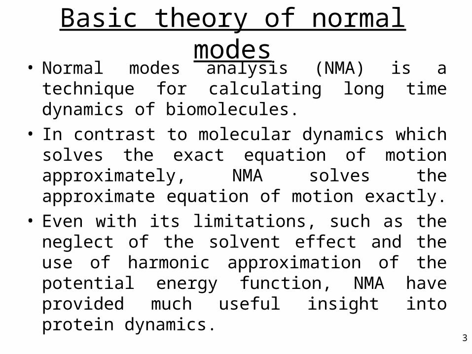
Basic theory of normal modes• Normal modes analysis (NMA) is a technique for

calculating long time dynamics of biomolecules.• In contrast to molecular dynamics which solves

the exact equation of motion approximately, NMA solves the approximate equation of motion exactly.

• Even with its limitations, such as the neglect of the solvent effect and the use of harmonic approximation of the potential energy function, NMA have provided much useful insight into protein dynamics.

4

Basic theory of normal modes (I)

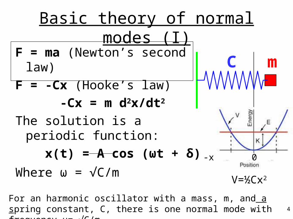
F = ma (Newton’s second law)

F = -Cx (Hooke’s law)

-Cx = m d2x/dt2

The solution is a periodic function:

x(t) = A cos (ωt + δ)

Where ω = √C/m

For an harmonic oscillator with a mass, m, and a spring constant, C, there is one normal mode with frequency ω= √C/m

mC

-x 0 x

V=½Cx2

5

C m C m C

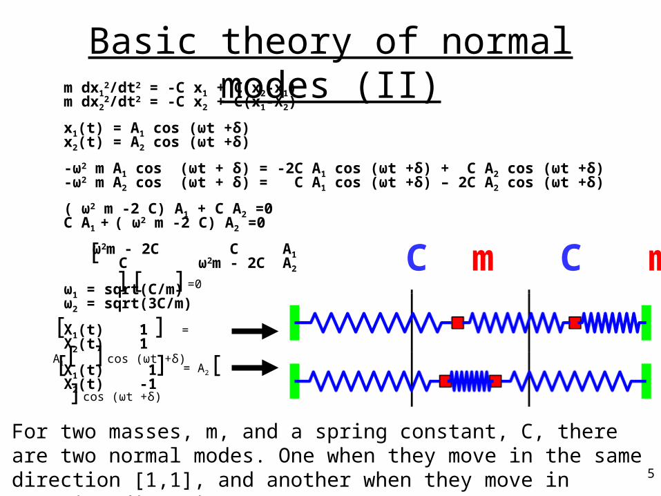
m dx12/dt2 = -C x1 + C(x2-x1)

m dx22/dt2 = -C x2 + C(x1-X2)

x1(t) = A1 cos (ωt +δ)x2(t) = A2 cos (ωt +δ)                                    -ω2 m A1 cos  (ωt + δ) = -2C A1 cos (ωt +δ) + C A2 cos (ωt +δ)-ω2 m A2 cos  (ωt + δ) = C A1 cos (ωt +δ) – 2C A2 cos (ωt +δ)

( ω2 m -2 C) A1 + C A2 =0C A1 + ( ω2 m -2 C) A2 =0

ω2m - 2C C A1 C ω2m - 2C A2

ω1 = sqrt(C/m)ω2 = sqrt(3C/m)

X1(t) 1X2(t)   1                                                    

X1(t) 1X2(t)   -1

[ ][ ]=0

[ ] = A1[ ]cos (ωt +δ)

[ ] = A2[ ]cos (ωt +δ)

Basic theory of normal modes (II)

For two masses, m, and a spring constant, C, there are two normal modes. One when they move in the same direction [1,1], and another when they move in opposite directions [1,-1].

6

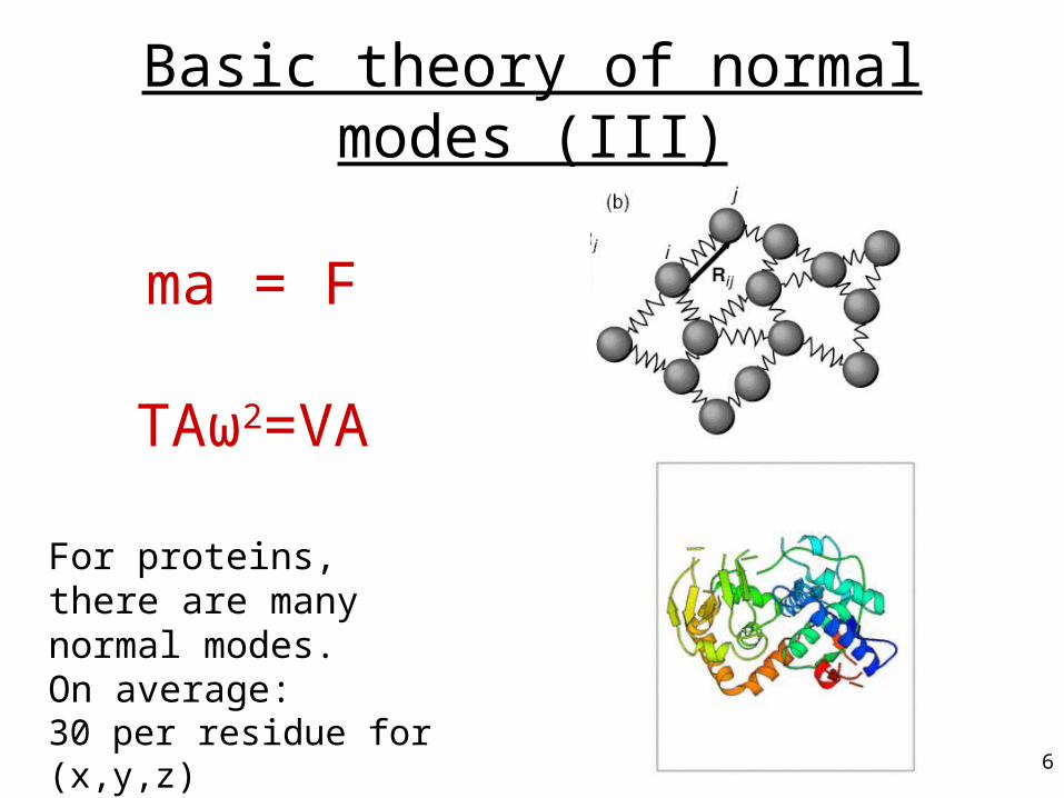
Basic theory of normal modes (III)

ma = F

TAω2=VA

For proteins, there are many normal modes. On average:30 per residue for (x,y,z)4 per residue for (φ,ψ,χ)

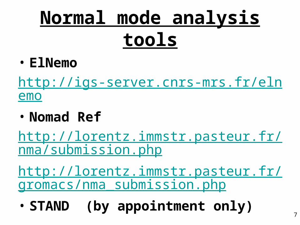
Normal mode analysis tools

• ElNemo

http://igs-server.cnrs-mrs.fr/elnemo

• Nomad Ref

http://lorentz.immstr.pasteur.fr/nma/submission.php

http://lorentz.immstr.pasteur.fr/gromacs/nma_submission.php

• STAND (by appointment only)

7

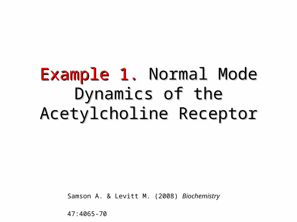
Example 1.Example 1. Normal Mode Dynamics Normal Mode Dynamics of the Acetylcholine Receptorof the Acetylcholine Receptor

Samson A. & Levitt M. (2008) Biochemistry 47:4065-70

9

Normal mode of acetylcholine receptor

•The receptor displays an twist like motion, responsible for the axially symmetric opening and closing of the ion channel

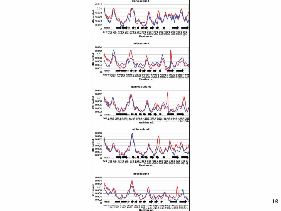
10

11

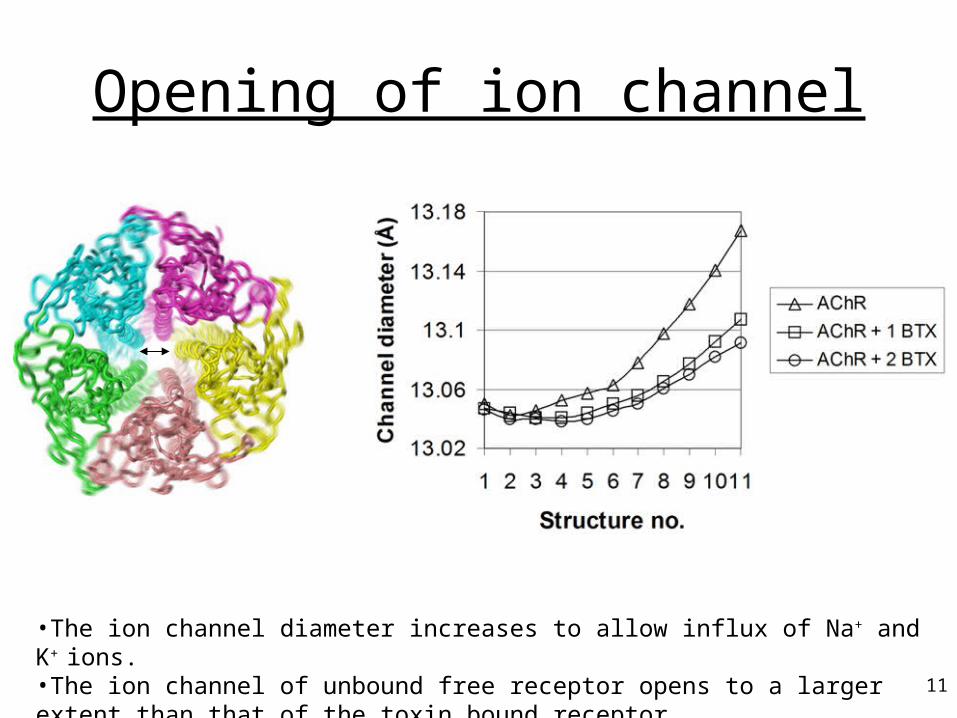
Opening of ion channel

•The ion channel diameter increases to allow influx of Na+ and K+ ions. •The ion channel of unbound free receptor opens to a larger extent than that of the toxin bound receptor.

12

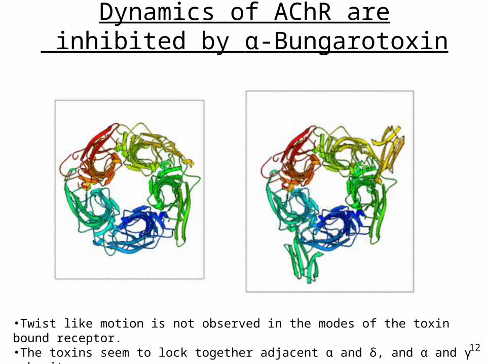
Dynamics of AChR are inhibited by α-Bungarotoxin

•Twist like motion is not observed in the modes of the toxin bound receptor. •The toxins seem to lock together adjacent α and δ, and α and γ subunits •One toxin is sufficient to prevent the opening motion.

Example 2.Example 2. Normal Mode Dynamics Normal Mode Dynamics of Prion Proteinsof Prion Proteins

Samson A. & Levitt M. (2011) Biochemistry 50:2243-8

14

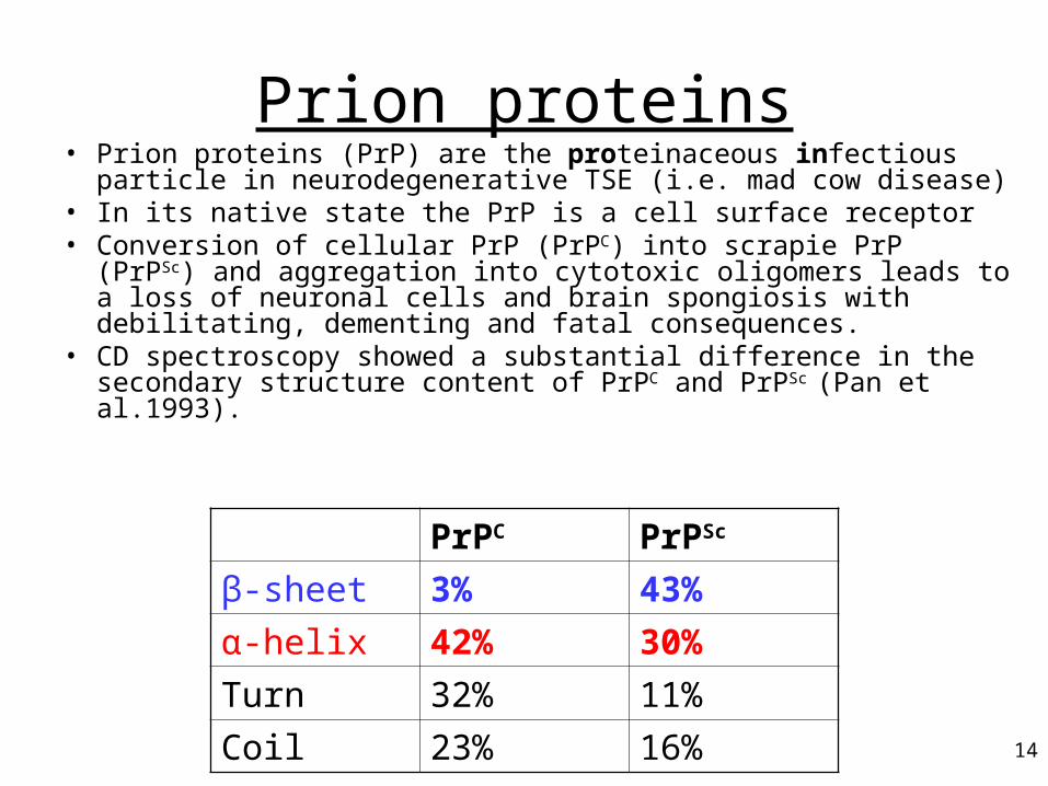
Prion proteins• Prion proteins (PrP) are the proteinaceous infectious particle in

neurodegenerative TSE (i.e. mad cow disease)• In its native state the PrP is a cell surface receptor • Conversion of cellular PrP (PrPC) into scrapie PrP (PrPSc) and

aggregation into cytotoxic oligomers leads to a loss of neuronal cells and brain spongiosis with debilitating, dementing and fatal consequences.

• CD spectroscopy showed a substantial difference in the secondary structure content of PrPC and PrPSc (Pan et al.1993).

PrPC PrPSc

β-sheet 3% 43%

α-helix 42% 30%

Turn 32% 11%

Coil 23% 16%

15

_________________________________________________________________ . . . . . SEQ 125 LGGYMLGSAMSRPIIHFGSDYEDRYYRENMHRYPNQVYYRPMDEYSNQNN 174 Native EE HHHHHHHHHHGGG EE GGGGG HHH Distorted EE HHHHHHHHHHGGG EE GGGGG HHH . . . . . SEQ 175 FVHDCVNITIKQHTVTTTTKGENFTETDVKMMERVVEQMCITQYERESQA 224 Native HHHHHHHHHHHHHHHHHHH HHHHHHHHHHHHHHHHHHHHHHHHH Distorted HHHHHHHHHHHHHHHHHHH HHHHHHHHHHHHHHHHHHHHHHHH _________________________________________________________________

(PDB ID 3HES)

Normal mode of M129 prion (WT)

16

Normal mode of V129 prion (variant)

_________________________________________________________________ . . . . . SEQ 125 LGGYVLGSAMSRPIIHFGSDYEDRYYRENMHRYPNQVYYRPMDEYSNQNN 174 Native EE HHHHHHHHHHGGG EE GGGGG HHH Distorted EEEEE HHHHHHHGGG EEEEE GGGGG HHH . . . . . SEQ 175 FVHDCVNITIKQHTVTTTTKGENFTETDVKMMERVVEQMCITQYERESQA 224 Native HHHHHHHHHHHHHHHHHHH HHHHHHHHHHHHHHHHHHHHHHHHH Distorted HHHHHHHHHHHHHHHHHHH HHHHHHHHHHHHHHHHHHHHHHHH _________________________________________________________________

(PDB ID 3HAK)

Trajectory path using NMA

http://lorentz.immstr.pasteur.fr/joel/index.php

Coiled coils of hemagglutinin!

17

Molecular dynamics

Molecular dynamics

• Why simulate motion of molecules?

• Energy model of conformation

• Two main approaches:– Monte Carlo - stochastic– Molecular dynamics - deterministic

• Applications of MD

• Speeding up MD

19

Why simulate motion?

• Predict structure• Understand interactions• Understand properties• Learn about normal modes of vibration• Design of bio-nano materials• Experiment on what cannot be studied

experimentally• Obtain a movie of the interacting molecules

20

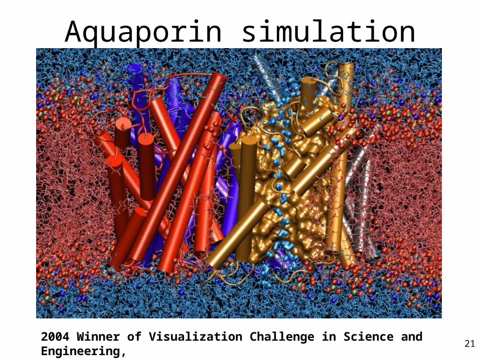
Aquaporin simulation

2004 Winner of Visualization Challenge in Science and Engineering, Organized by the National Science Foundation and Science Magazine.

21

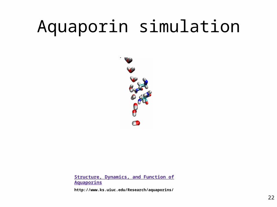
Aquaporin simulation

Structure, Dynamics, and Function of Aquaporins

http://www.ks.uiuc.edu/Research/aquaporins/

22

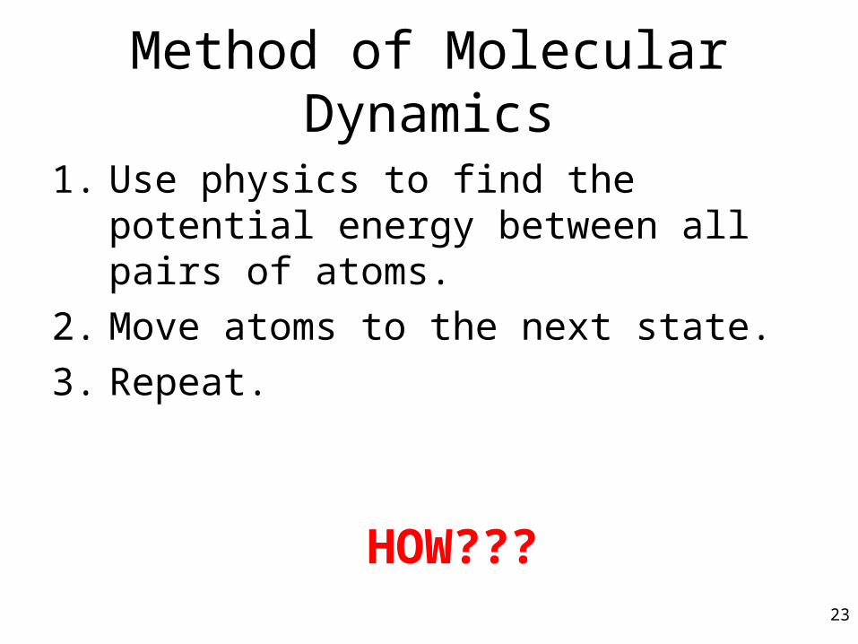
Method of Molecular Dynamics

1. Use physics to find the potential energy between all pairs of atoms.

2. Move atoms to the next state.

3. Repeat.

HOW???23

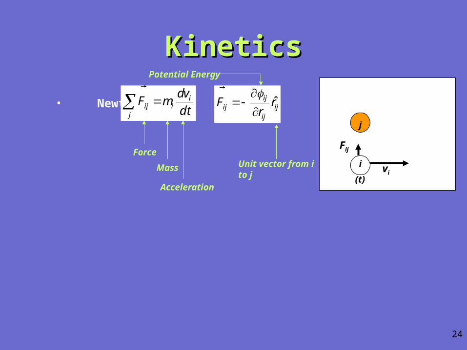
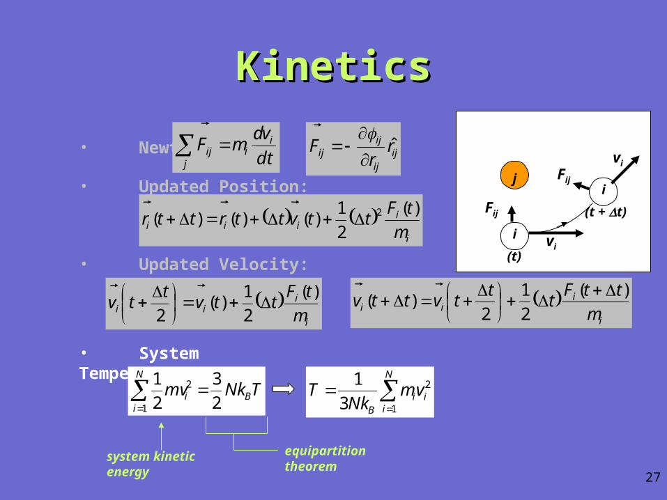
• Newton:dt

vdmF i

ij

ij

ij

ij

ijij r

rF ˆ

i

j

Fij

vi(t)

Force

Mass

Acceleration

Potential Energy

Unit vector from i to j

KineticsKinetics

24

• Newton:dt

vdmF i

ij

ij

ij

ij

ijij r

rF ˆ

• Updated Position:

i

iiii m

tFttvttrttr

)(

2

1)()()( 2

new position old

position old velocity

old force

KineticsKinetics

i

Fij

vi

i

(t)

(t + t)

j

25

• Newton:dt

vdmF i

ij

ij

ij

ij

ijij r

rF ˆ

• Updated Position:

i

iiii m

tFttvttrttr

)(

2

1)()()( 2

• Updated Velocity:

i

iii m

tFttv

ttv

)(

2

1)(

2

i

iii m

ttFt

ttvttv

)(

2

1

2)(

first half of time step second half of time step

KineticsKinetics

i

Fij

vi

i

(t)

Fij

vi

(t + t)

j

26

• Newton:dt

vdmF i

ij

ij

ij

ij

ijij r

rF ˆ

• Updated Position:

i

iiii m

tFttvttrttr

)(

2

1)()()( 2

• Updated Velocity:

i

iii m

tFttv

ttv

)(

2

1)(

2

i

iii m

ttFt

ttvttv

)(

2

1

2)(

• System Temperature:

TNkmv B

N

ii 2

3

2

1

1

2

N

iii

B

vmNk

T1

2

3

1

system kinetic energy

equipartition theorem

KineticsKinetics

i

Fij

vi

i

(t)

Fij

vi

(t + t)

j

27

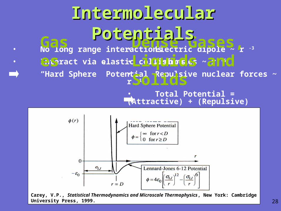
Carey, V.P., Statistical Thermodynamics and Microscale Thermophysics, New York: Cambridge University Press, 1999.

• No long range interactions

• Interact via elastic collisions

“Hard Sphere” Potential

Gases

• Electric dipole ~ r -3

• 2 dipoles ~ r -6

• Repulsive nuclear forces ~ r -12

• Total Potential = (Attractive) + (Repulsive)

“Lennard-Jones 6-12 Potential”

Dense Gases, Liquids and Solids

Intermolecular PotentialsIntermolecular Potentials

28

Energy Function

• Target function that MD tries to optimize

• Describes the interaction energies of all atoms and molecules in the system

• Always an approximation– Closer to real physics --> more realistic, more

computation time (I.e. smaller time steps and more interactions increase accuracy)

29

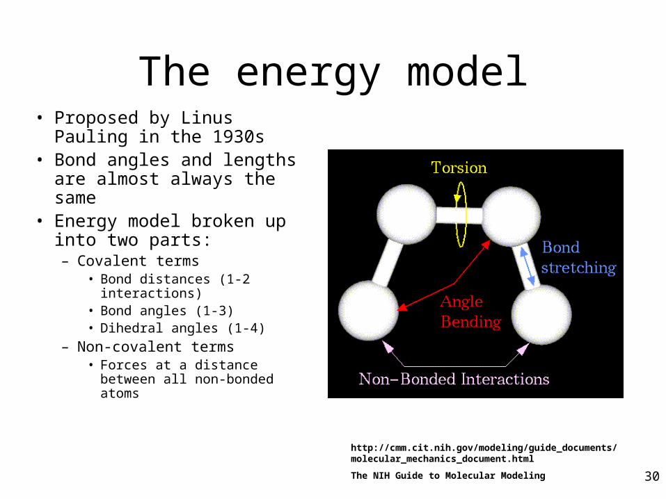
The energy model

http://cmm.cit.nih.gov/modeling/guide_documents/molecular_mechanics_document.html

The NIH Guide to Molecular Modeling

• Proposed by Linus Pauling in the 1930s

• Bond angles and lengths are almost always the same

• Energy model broken up into two parts:– Covalent terms

• Bond distances (1-2 interactions)

• Bond angles (1-3)• Dihedral angles (1-4)

– Non-covalent terms• Forces at a distance between

all non-bonded atoms

30

The energy equation

Energy =

Stretching Energy +

Bending Energy +

Torsion Energy +

Non-Bonded Interaction Energy

These equations together with the data (parameters) required to describe the behavior of different kinds of atoms and bonds, is called a force-field.

31

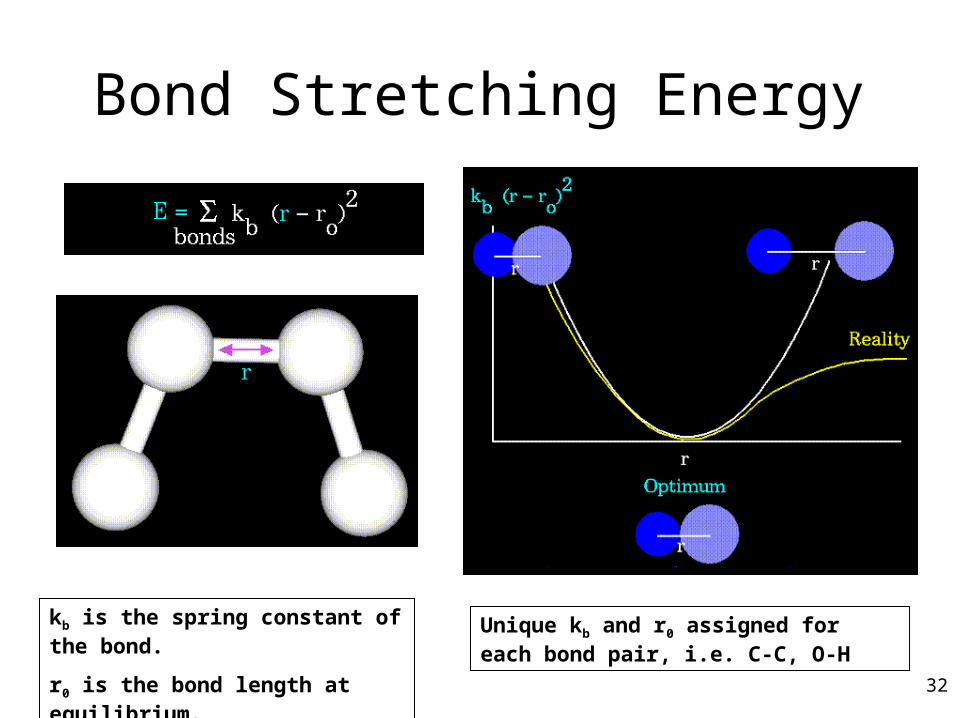
Bond Stretching Energy

kb is the spring constant of the bond.

r0 is the bond length at equilibrium.

Unique kb and r0 assigned for each bond pair, i.e. C-C, O-H

32

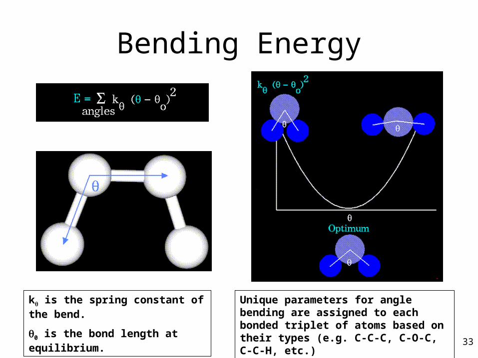
Bending Energy

k is the spring constant of the bend.

0 is the bond length at equilibrium.

Unique parameters for angle bending are assigned to each bonded triplet of atoms based on their types (e.g. C-C-C, C-O-C, C-C-H, etc.) 33

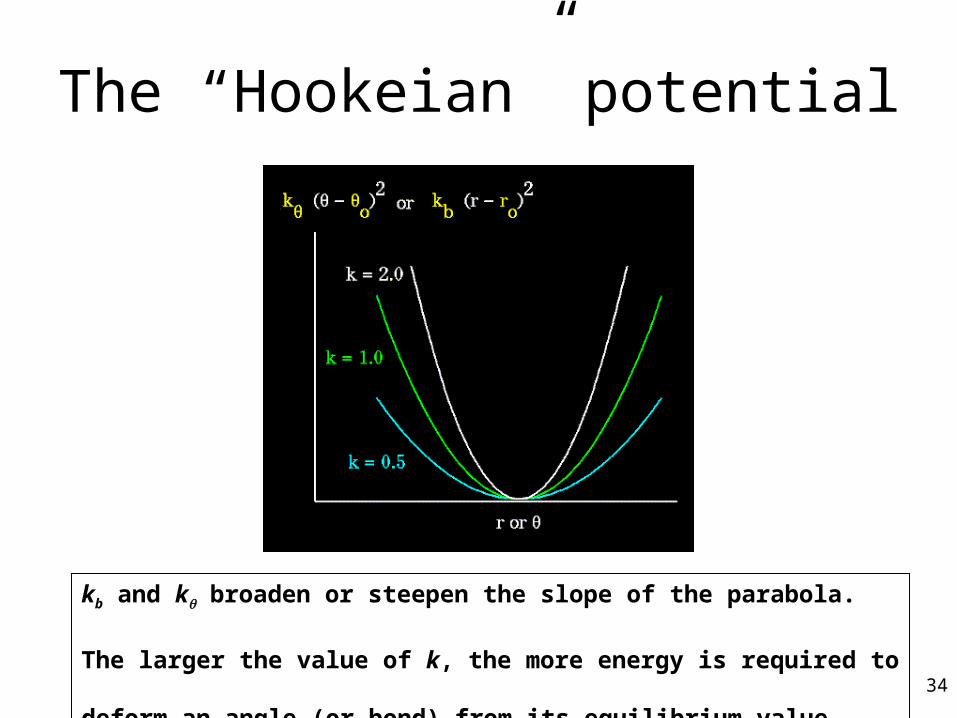
The “Hookeian” potential

kb and k broaden or steepen the slope of the parabola.

The larger the value of k, the more energy is required to deform an

angle (or bond) from its equilibrium value. 34

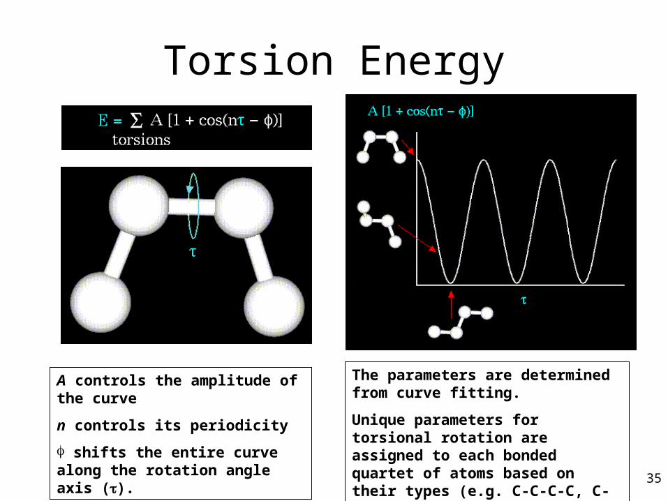
Torsion Energy

A controls the amplitude of the curve

n controls its periodicity

shifts the entire curve along the rotation angle axis ().

The parameters are determined from curve fitting.

Unique parameters for torsional rotation are assigned to each bonded quartet of atoms based on their types (e.g. C-C-C-C, C-O-C-N, H-C-C-H, etc.) 35

Torsion Energy parameters

A is the amplitude.

n reflects the type symmetry in the dihedral angle.

used to synchronize the torsional potential to the initial rotameric state of the molecule

36

Non-bonded Energy

A determines the degree the attractiveness

B determines the degree of repulsion

q is the charge

A determines the degree the attractiveness

B determines the degree of repulsion

q is the charge37

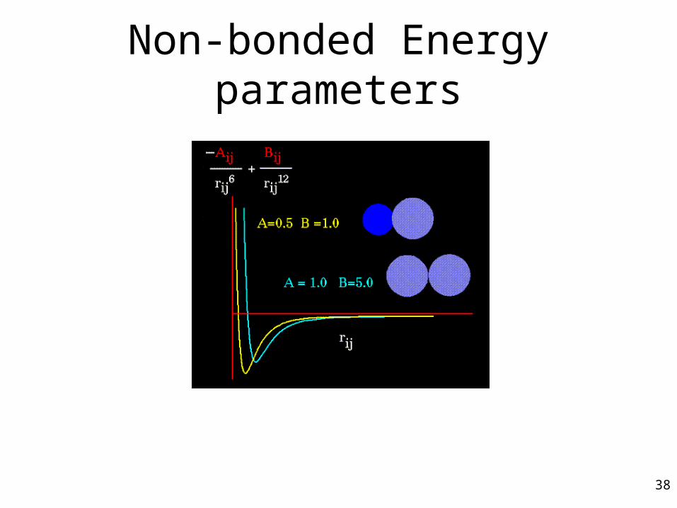
Non-bonded Energy parameters

38

Simulating In A Solvent• The smaller the system, the more particles on

the surface– 1000 atom cubic crystal, 49% on surface

– 10^6 atom cubic crystal, 6% on surface

• Would like to simulate infinite bulk surrounding N-particle system

• Two approaches:– Implicitly– Explicitly

• Ex. Periodic boundary conditions

Schematic representation of periodic boundary conditions.

http://www.ccl.net/cca/documents/molecular-modeling/node9.html

40

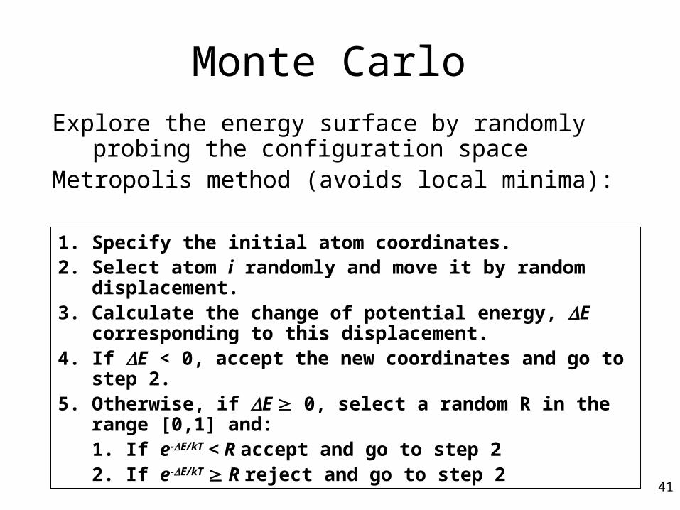
Monte CarloExplore the energy surface by randomly probing

the configuration spaceMetropolis method (avoids local minima):

1. Specify the initial atom coordinates.2. Select atom i randomly and move it by random

displacement.3. Calculate the change of potential energy, E corresponding

to this displacement.4. If E < 0, accept the new coordinates and go to step 2.5. Otherwise, if E 0, select a random R in the range [0,1]

and:1. If e-E/kT < R accept and go to step 2 2. If e-E/kT R reject and go to step 2

41

Properties of MC simulation

• System behaves as a Markov process– Current state depends only on previous.– Converges quickly.

• System is ergodic (any state can be reached from any other state).

• Accepted more by physicists than by chemists.– Not deterministic and does not offer time evolution of

the system.

42

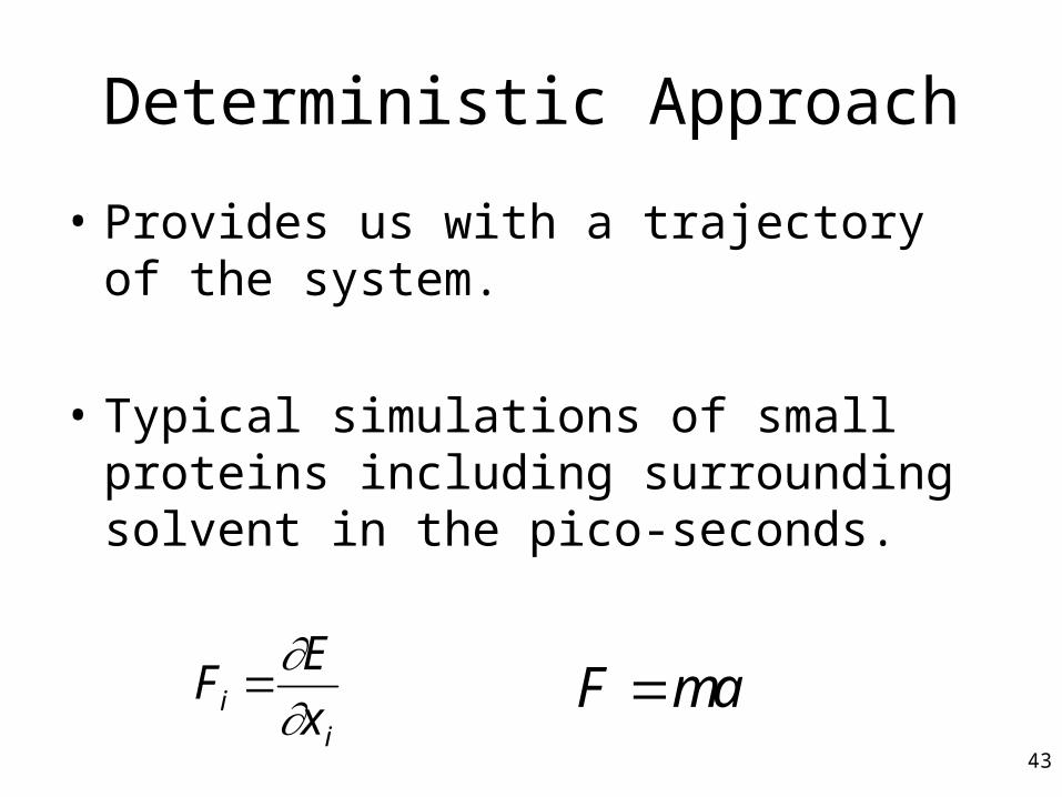
Deterministic Approach

• Provides us with a trajectory of the system.

• Typical simulations of small proteins including surrounding solvent in the pico-seconds.

Fi E

x i

F m

a

43

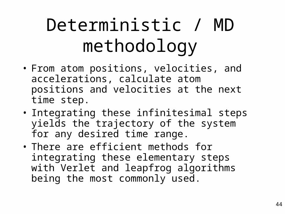
Deterministic / MD methodology

• From atom positions, velocities, and accelerations, calculate atom positions and velocities at the next time step.

• Integrating these infinitesimal steps yields the trajectory of the system for any desired time range.

• There are efficient methods for integrating these elementary steps with Verlet and leapfrog algorithms being the most commonly used.

44

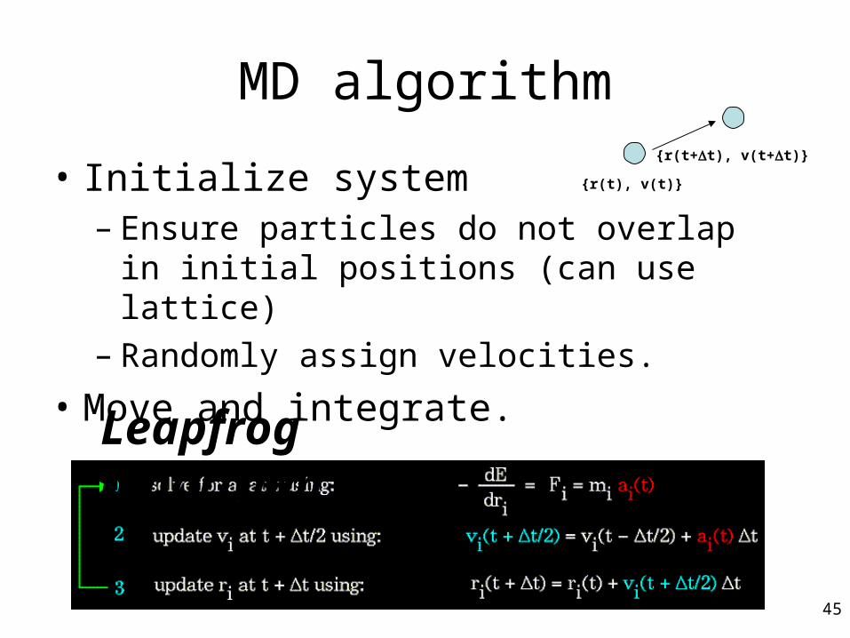
MD algorithm

• Initialize system– Ensure particles do not overlap in initial

positions (can use lattice)– Randomly assign velocities.

• Move and integrate.

{r(t), v(t)}

{r(t+t), v(t+t)}

Leapfrog algorithm

45