Embed Size (px)
Citation preview
Motivation and Methods in
Earth System Data Assimilation
ECMWF Annual Seminar
Mark Buehner
Data Assimilation and Satellite
Meteorology Research
10-13 September 2018
Page 2 – September 11, 2018
Outline
• Motivation: The need for Earth System Data Assimilation
• Methods:
– DA Methods used for NWP, including hybrid methods
– DA Methods for other geophysical components: e.g. Sea ice
– Methods for coupled DA
• Examples:
– First attempts at coupled Atmosphere-Ice-Ocean DA at ECCC
• Strategy for Earth System DA at ECCC
– Use of highly modular common DA software for all components
– Explore scale-dependent combined with system-dependent ensemble covariance localization
Page 3 – September 11, 2018
Outline
• Motivation: The need for Earth System Data Assimilation
• Methods:
– DA Methods used for NWP, including hybrid methods
– DA Methods for other geophysical components
– Methods for coupled DA
• Examples:
– First attempts at coupled Atmosphere-Ice-Ocean DA at ECCC
• Strategy for Earth System DA at ECCC
– Use of highly modular common DA software for all components
– Explore scale-dependent combined with system-dependent ensemble covariance localization
Page 4 – September 11, 2018
Motivation: Earth System Prediction
• Operational forecast models increasingly coupled (2016 Annual Seminar; ECCC global forecasts coupled with Ice-Ocean since November, 2017)
• Benefits from coupled forecasts even at shorter time-scales relevant for medium-range NWP, related to:
– Tropical convection,
– Hurricanes, extra-tropical storms
– Coastal upwelling,
– Sea ice (polynyas, leads)
• Additional benefits from providing operational ice-ocean forecasts and services – may require new collaborations (e.g. Canadian Ice Service)
• Initialization of these models from independent assimilation systems for each component a challenge
Page 5 – September 11, 2018
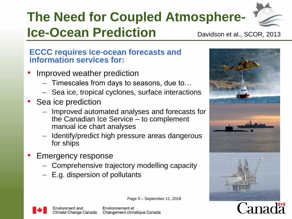
The Need for Coupled Atmosphere-
Ice-Ocean Prediction
• Improved weather prediction – Timescales from days to seasons, due to…
– Sea ice, tropical cyclones, surface interactions
• Sea ice prediction – Improved automated analyses and forecasts for
the Canadian Ice Service – to complement manual ice chart analyses
– Identify/predict high pressure areas dangerous for ships
• Emergency response – Comprehensive trajectory modelling capacity
– E.g. dispersion of pollutants
ECCC requires ice-ocean forecasts and information services for:
Davidson et al., SCOR, 2013
Page 6 – September 11, 2018
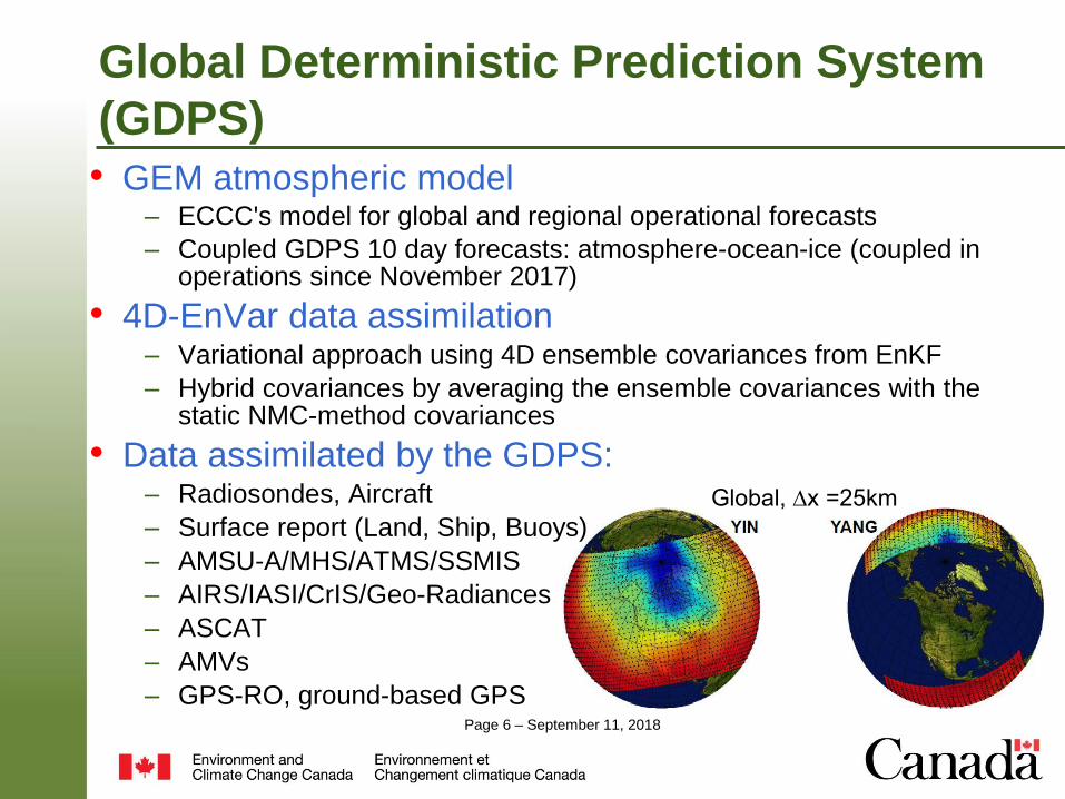
Global Deterministic Prediction System
(GDPS)
Global, ∆x =25km
• GEM atmospheric model – ECCC's model for global and regional operational forecasts
– Coupled GDPS 10 day forecasts: atmosphere-ocean-ice (coupled in operations since November 2017)
• 4D-EnVar data assimilation– Variational approach using 4D ensemble covariances from EnKF
– Hybrid covariances by averaging the ensemble covariances with the static NMC-method covariances
• Data assimilated by the GDPS:– Radiosondes, Aircraft
– Surface report (Land, Ship, Buoys)
– AMSU-A/MHS/ATMS/SSMIS
– AIRS/IASI/CrIS/Geo-Radiances
– ASCAT
– AMVs
– GPS-RO, ground-based GPS
Page 7 – September 11, 2018
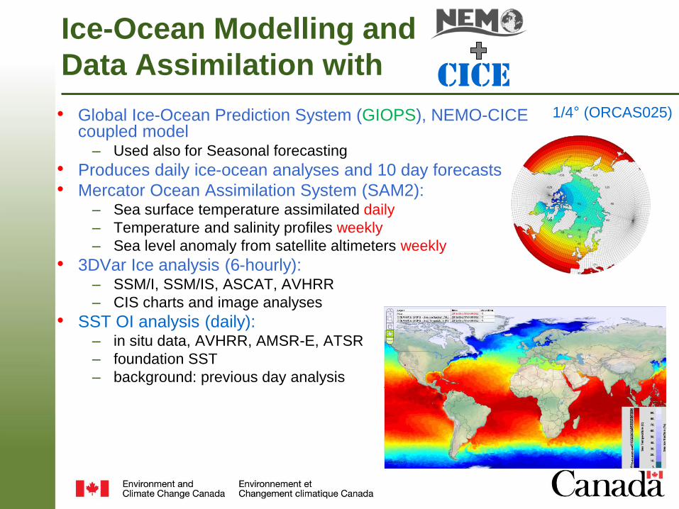
Ice-Ocean Modelling and
Data Assimilation with
1/4° (ORCAS025)• Global Ice-Ocean Prediction System (GIOPS), NEMO-CICE coupled model
– Used also for Seasonal forecasting
• Produces daily ice-ocean analyses and 10 day forecasts
• Mercator Ocean Assimilation System (SAM2):– Sea surface temperature assimilated daily
– Temperature and salinity profiles weekly
– Sea level anomaly from satellite altimeters weekly
• 3DVar Ice analysis (6-hourly):– SSM/I, SSM/IS, ASCAT, AVHRR
– CIS charts and image analyses
• SST OI analysis (daily):– in situ data, AVHRR, AMSR-E, ATSR
– foundation SST
– background: previous day analysis
CICE
Page 8 – September 11, 2018
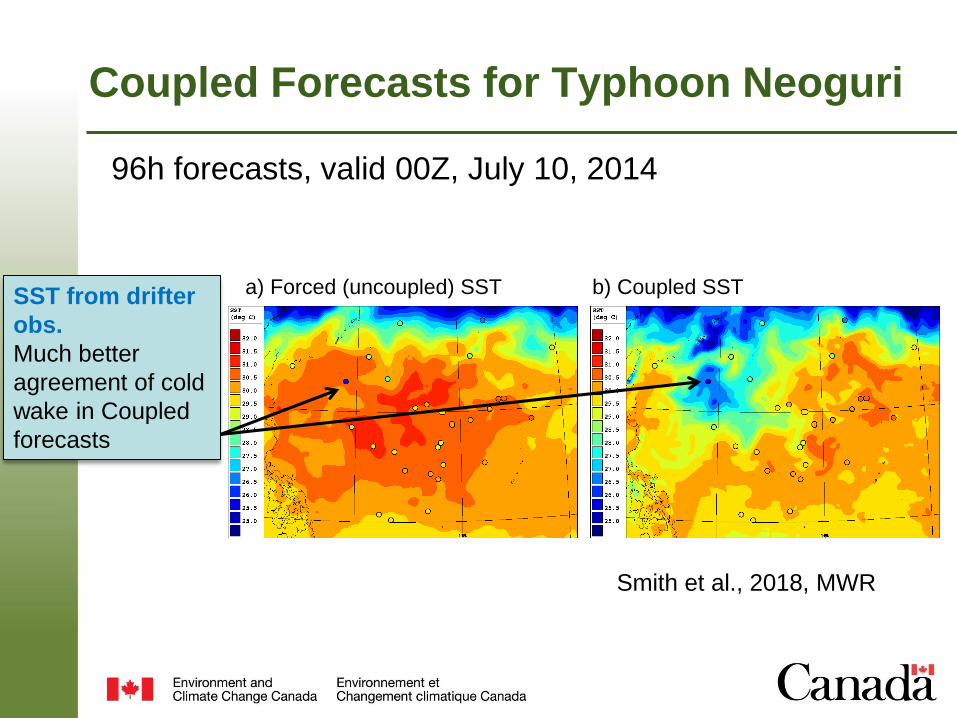
Coupled Forecasts for Typhoon Neoguri
96h forecasts, valid 00Z, July 10, 2014
a) Forced (uncoupled) SST b) Coupled SSTSST from drifter
obs.
Much better
agreement of cold
wake in Coupled
forecasts
Smith et al., 2018, MWR
Page 9 – September 11, 2018
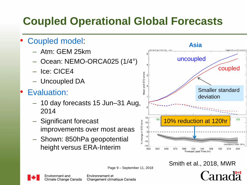
Coupled Operational Global Forecasts
• Coupled model:
– Atm: GEM 25km
– Ocean: NEMO-ORCA025 (1/4°)
– Ice: CICE4
– Uncoupled DA
• Evaluation:
– 10 day forecasts 15 Jun–31 Aug,
2014
– Significant forecast
improvements over most areas
– Shown: 850hPa geopotential
height versus ERA-Interim
coupled
uncoupled
Smaller standard
deviation
Asia
10% reduction at 120hr
Smith et al., 2018, MWR
Page 10 – September 11, 2018
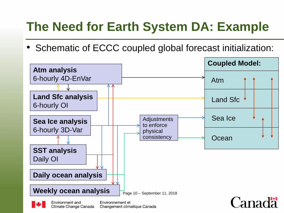
The Need for Earth System DA: Example
• Schematic of ECCC coupled global forecast initialization:
Coupled Model:
Atm
Land Sfc
Sea Ice
Ocean
SST analysis
Daily OI
Sea Ice analysis
6-hourly 3D-Var
Atm analysis
6-hourly 4D-EnVar
Land Sfc analysis
6-hourly OI
Daily ocean analysis
Weekly ocean analysis
Adjustments to enforce physical consistency
Page 11 – September 11, 2018
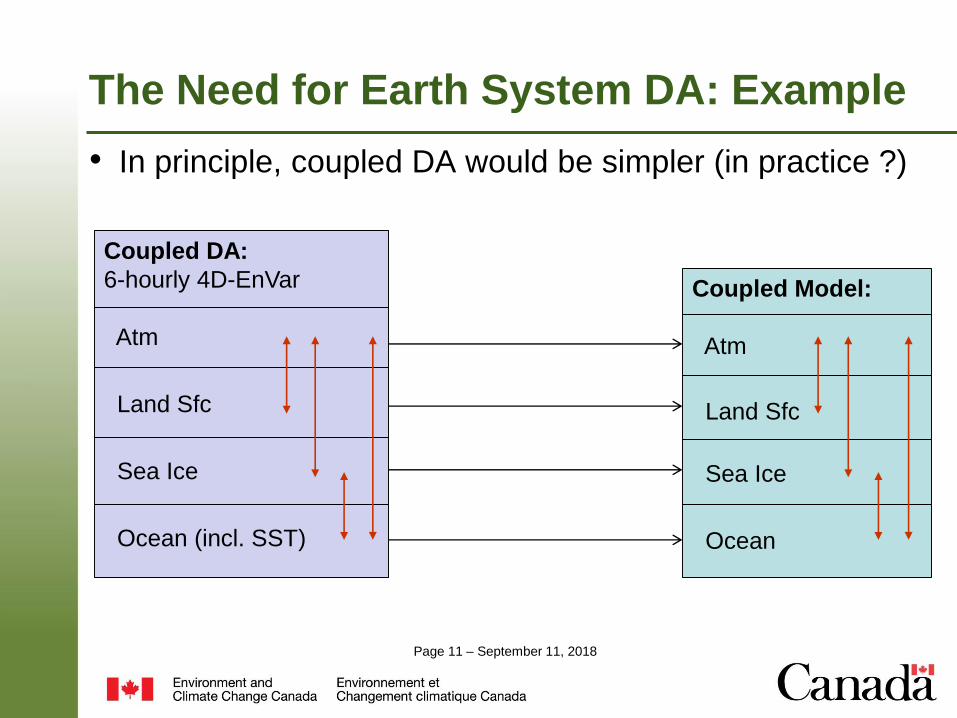
The Need for Earth System DA: Example
• In principle, coupled DA would be simpler (in practice ?)
Coupled Model:
Atm
Land Sfc
Sea Ice
Ocean
Coupled DA:
6-hourly 4D-EnVar
Atm
Land Sfc
Sea Ice
Ocean (incl. SST)
Page 12 – September 11, 2018
The Need for Coupled Earth System DA
• Several challenges in initializing coupled models could be handled more directly with coupled assimilation methods
• Better treatment of physical consistency between component systems:
– Analysis updates to sea-ice and ocean temperature, consistency essential for even short-term sea ice forecasts
– Background errors of near-surface atmosphere can be highly correlated with ocean/land surface errors
• Accounting for background error correlations between component systems allows observations of one component to correct another
• Consistent assimilation of "coupled" observations:
– Many surface-sensitive satellite observations used for extracting sea ice and ocean information also sensitive to atmosphere (e.g. estimating sea ice concentration with an RTM, Scott et al. 2012)
– Location of sea-ice edge affects selection/usage of surface-sensitive atmospheric and ocean observations
Page 13 – September 11, 2018
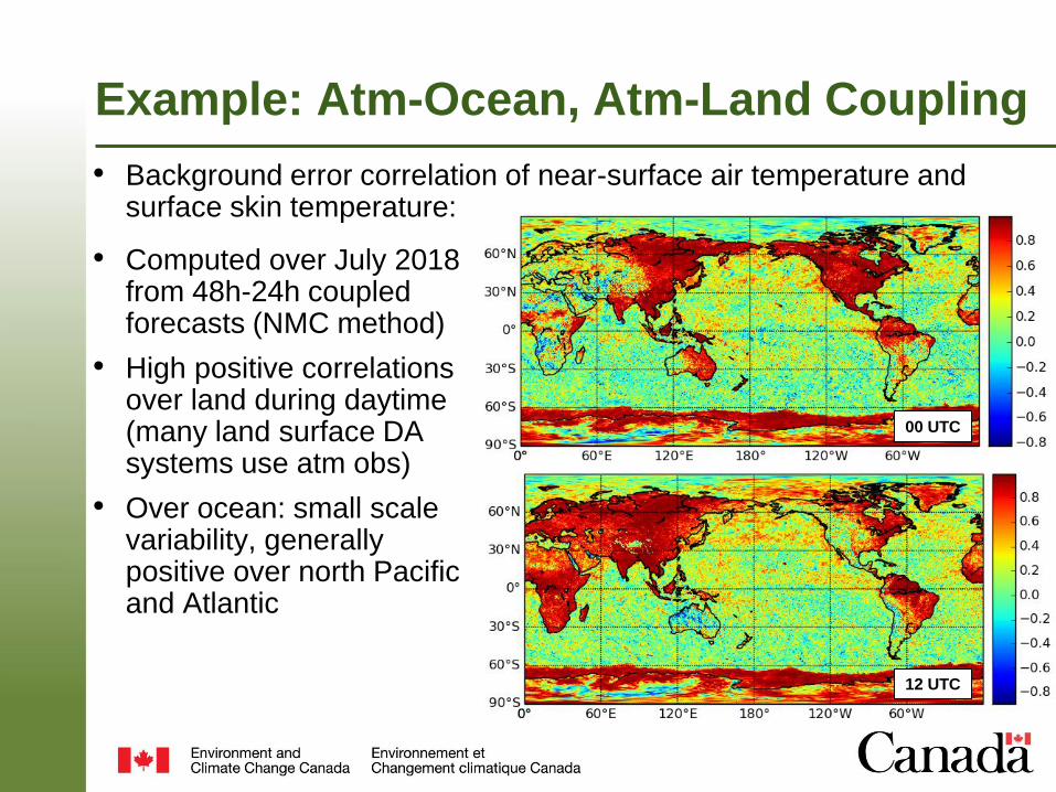
Example: Atm-Ocean, Atm-Land Coupling
• Background error correlation of near-surface air temperature and surface skin temperature:
• Computed over July 2018 from 48h-24h coupled forecasts (NMC method)
• High positive correlations over land during daytime (many land surface DA systems use atm obs)
• Over ocean: small scale variability, generally positive over north Pacific and Atlantic
00 UTC
12 UTC
Page 14 – September 11, 2018
Outline
• Motivation: The need for Earth System Data Assimilation
• Methods:
– DA Methods used for NWP, including hybrid methods
– DA Methods for other geophysical components: e.g. Sea ice
– Methods for coupled DA
• Examples:
– First attempts at coupled Atmosphere-Ice-Ocean DA at ECCC
• Strategy for Earth System DA at ECCC
Page 15 – September 11, 2018
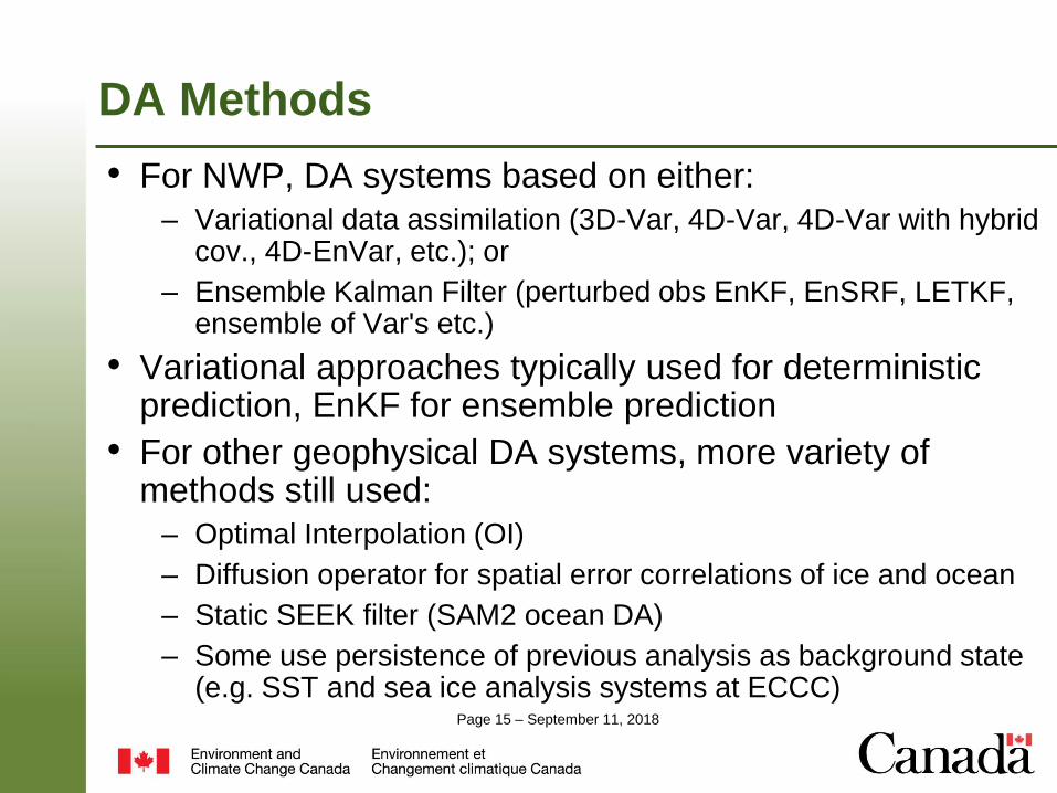
• For NWP, DA systems based on either:
– Variational data assimilation (3D-Var, 4D-Var, 4D-Var with hybrid cov., 4D-EnVar, etc.); or
– Ensemble Kalman Filter (perturbed obs EnKF, EnSRF, LETKF, ensemble of Var's etc.)
• Variational approaches typically used for deterministic prediction, EnKF for ensemble prediction
• For other geophysical DA systems, more variety of methods still used:
– Optimal Interpolation (OI)
– Diffusion operator for spatial error correlations of ice and ocean
– Static SEEK filter (SAM2 ocean DA)
– Some use persistence of previous analysis as background state (e.g. SST and sea ice analysis systems at ECCC)
DA Methods
Page 16 – September 11, 2018
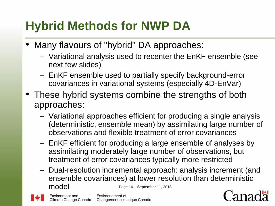
Hybrid Methods for NWP DA
• Many flavours of "hybrid" DA approaches:
– Variational analysis used to recenter the EnKF ensemble (see next few slides)
– EnKF ensemble used to partially specify background-error covariances in variational systems (especially 4D-EnVar)
• These hybrid systems combine the strengths of both approaches:
– Variational approaches efficient for producing a single analysis (deterministic, ensemble mean) by assimilating large number of observations and flexible treatment of error covariances
– EnKF efficient for producing a large ensemble of analyses by assimilating moderately large number of observations, but treatment of error covariances typically more restricted
– Dual-resolution incremental approach: analysis increment (and ensemble covariances) at lower resolution than deterministic model
Page 17 – September 11, 2018
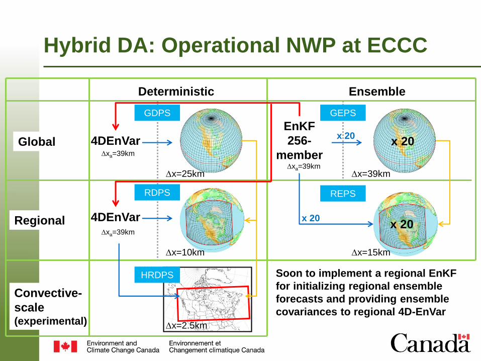
Hybrid DA: Operational NWP at ECCC
x 20
x 20Global
Regional
Convective-
scale(experimental)
Deterministic Ensemble
EnKF
256-
member
4DEnVar
4DEnVar
GDPS
RDPS
HRDPS
GEPS
REPS
x=10km
x=2.5km
x=39km
x=15km
xa=39km
xa=39km
xa=39km
x 20
x 20
x=25km
Soon to implement a regional EnKF
for initializing regional ensemble
forecasts and providing ensemble
covariances to regional 4D-EnVar
Page 18 – September 11, 2018
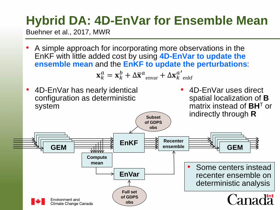
GEMGEMGEMGEMGEM
• A simple approach for incorporating more observations in the EnKF with little added cost by using 4D-EnVar to update the ensemble mean and the EnKF to update the perturbations:
𝐱𝑘𝑎 = 𝐱𝑘
𝑏 + ∆ത𝐱𝑎envar+ ∆𝐱𝑘𝑎′
enkf
Hybrid DA: 4D-EnVar for Ensemble MeanBuehner et al., 2017, MWR
EnKF
EnVar
GEMGEMGEMGEMGEM
Compute
mean
Recenter
ensemble
Full set
of GDPS
obs
Subset
of GDPS
obs
• 4D-EnVar has nearly identical configuration as deterministic system
• Some centers instead recenter ensemble on deterministic analysis
• 4D-EnVar uses direct spatial localization of Bmatrix instead of BHT or indirectly through R
Page 19 – September 11, 2018
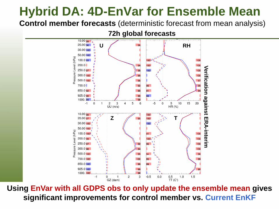
Hybrid DA: 4D-EnVar for Ensemble MeanControl member forecasts (deterministic forecast from mean analysis)
72h global forecasts
Using EnVar with all GDPS obs to only update the ensemble mean gives
significant improvements for control member vs. Current EnKF
Ve
rificatio
n a
ga
ins
t ER
A-in
terim
U
Z
RH
T
Page 20 – September 11, 2018
Hybrid Methods for Earth System DA
• Need to consider cost and complexity of expanding such DA systems to directly include other Earth system components:
– 4D-Var requires coding and maintaining TLM/AD versions of each component model, linearization for some geophysical models challenging due to nonlinearities (e.g. sea ice rheology)
– EnKF requires large ensemble size (~100 members) to estimate error covariances lower resolution than deterministic model, not straightforward for ocean/sea-ice (e.g. Arctic archipelago)
– Additional effort and expertise required to maintain separate DA algorithms and software for each system component
Page 21 – September 11, 2018
Outline
• Motivation: The need for Earth System Data Assimilation
• Methods:
– DA Methods used for NWP, including hybrid methods
– DA Methods for other geophysical components: e.g. Sea ice
– Methods for coupled DA
• Examples:
– First attempts at coupled Atmosphere-Ice-Ocean DA at ECCC
• Strategy for Earth System DA at ECCC
Page 22 – September 11, 2018
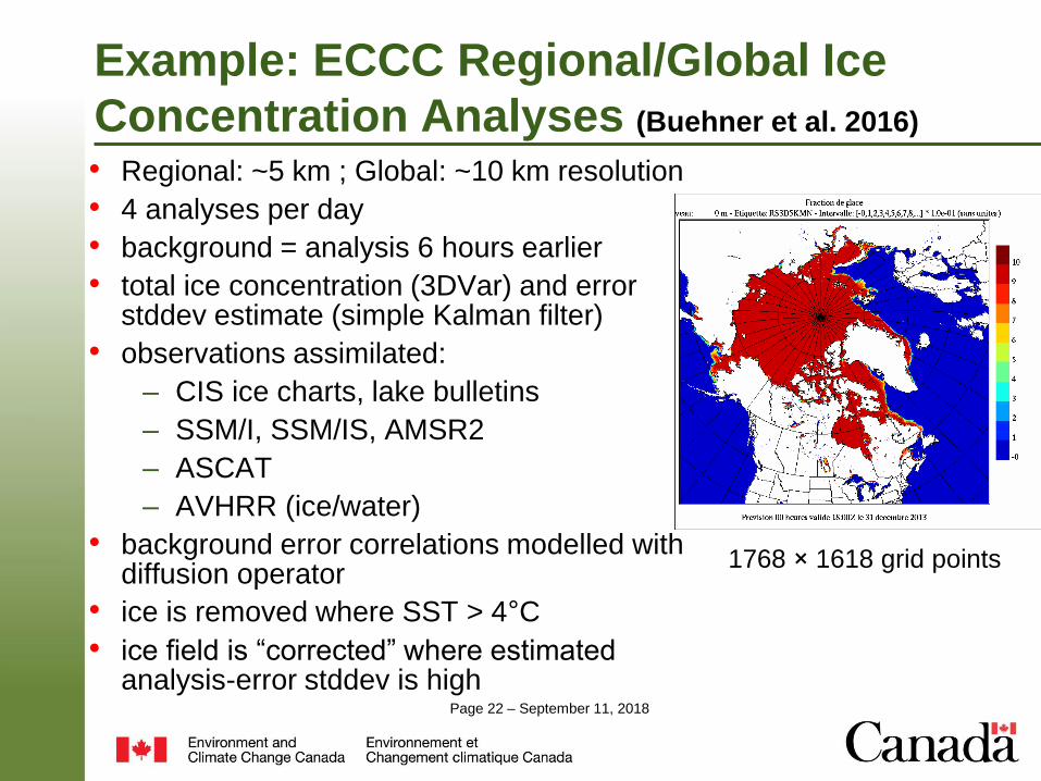
Example: ECCC Regional/Global Ice
Concentration Analyses (Buehner et al. 2016)
• Regional: ~5 km ; Global: ~10 km resolution
• 4 analyses per day
• background = analysis 6 hours earlier
• total ice concentration (3DVar) and error stddev estimate (simple Kalman filter)
• observations assimilated:
– CIS ice charts, lake bulletins
– SSM/I, SSM/IS, AMSR2
– ASCAT
– AVHRR (ice/water)
• background error correlations modelled with diffusion operator
• ice is removed where SST > 4°C
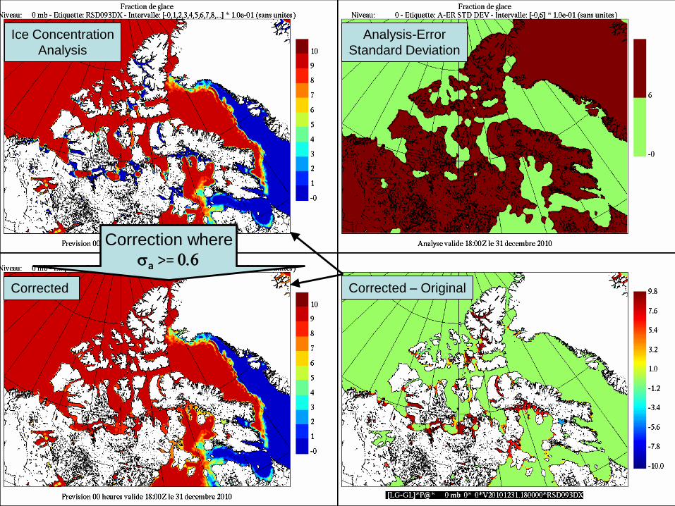
• ice field is “corrected” where estimated analysis-error stddev is high
1768 × 1618 grid points
Page 23 – September 11, 2018
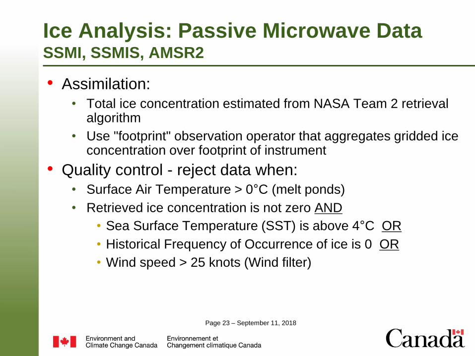
Ice Analysis: Passive Microwave DataSSMI, SSMIS, AMSR2
• Assimilation:
• Total ice concentration estimated from NASA Team 2 retrieval algorithm
• Use "footprint" observation operator that aggregates gridded ice concentration over footprint of instrument
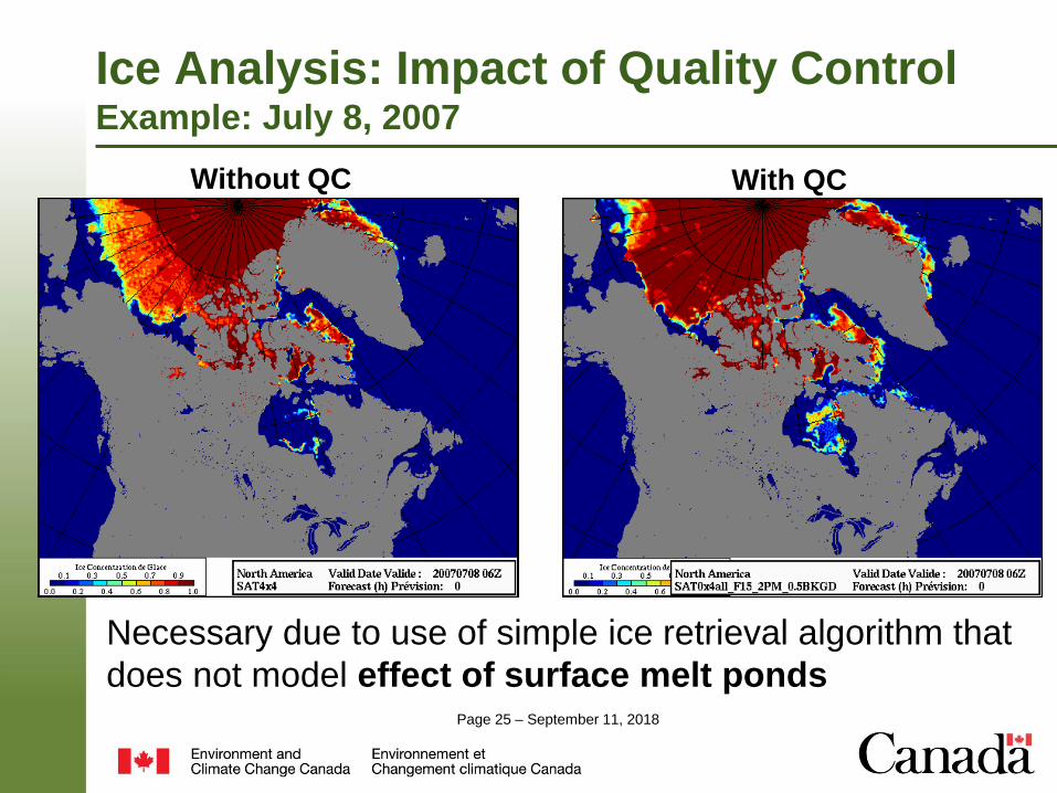
• Quality control - reject data when:
• Surface Air Temperature > 0°C (melt ponds)
• Retrieved ice concentration is not zero AND
• Sea Surface Temperature (SST) is above 4°C OR
• Historical Frequency of Occurrence of ice is 0 OR
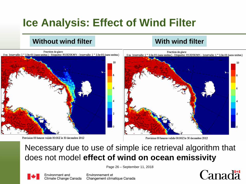
• Wind speed > 25 knots (Wind filter)
Page 24 – September 11, 2018
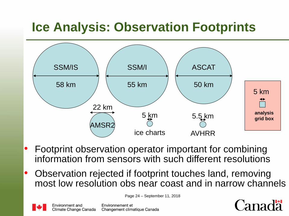
Ice Analysis: Observation Footprints
5 km
analysis
grid box
SSM/I
55 km
ASCAT
50 km
SSM/IS
58 km
AMSR2
22 km
5.5 km
AVHRR
5 km
ice charts
• Footprint observation operator important for combining information from sensors with such different resolutions
• Observation rejected if footprint touches land, removing most low resolution obs near coast and in narrow channels
Page 25 – September 11, 2018
Ice Analysis: Impact of Quality ControlExample: July 8, 2007
Without QC With QC
Necessary due to use of simple ice retrieval algorithm that
does not model effect of surface melt ponds
Page 26 – September 11, 2018
With wind filterWithout wind filter
Ice Analysis: Effect of Wind Filter
Necessary due to use of simple ice retrieval algorithm that
does not model effect of wind on ocean emissivity
Page 27 – September 11, 2018
Ice Concentration
Analysis
Analysis-Error
Standard Deviation
Corrected Corrected – Original
Correction where
sa >= 0.6
Page 28 – September 11, 2018
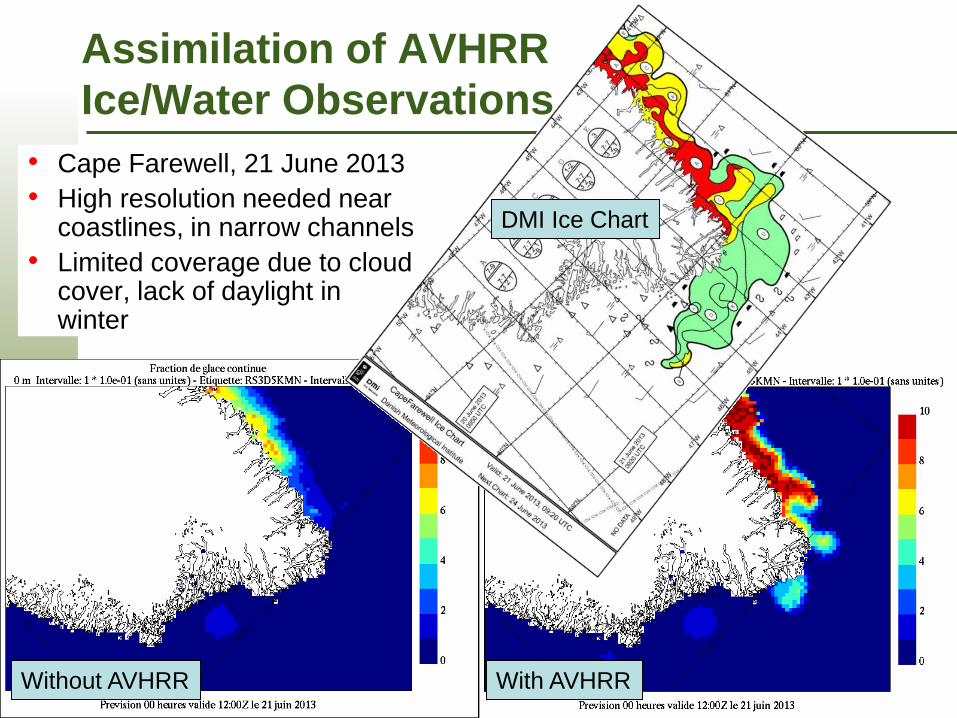
• Cape Farewell, 21 June 2013
• High resolution needed near coastlines, in narrow channels
• Limited coverage due to cloud cover, lack of daylight in winter
Without AVHRR With AVHRR
Assimilation of AVHRR
Ice/Water Observations
DMI Ice Chart
Page 29 – September 11, 2018
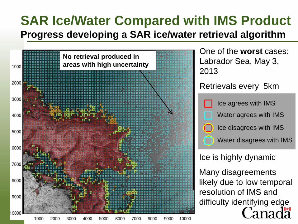
SAR Ice/Water Compared with IMS ProductProgress developing a SAR ice/water retrieval algorithm
One of the worst cases:
Labrador Sea, May 3,
2013
Retrievals every 5km
Ice agrees with IMS
Water agrees with IMS
Water disagrees with IMS
Ice disagrees with IMS
Ice is highly dynamic
Many disagreements
likely due to low temporal
resolution of IMS and
difficulty identifying edge
No retrieval produced in
areas with high uncertainty
Page 30 – September 11, 2018
Outline
• Motivation: The need for Earth System Data Assimilation
• Methods:
– DA Methods used for NWP, including hybrid methods
– DA Methods for other geophysical components: e.g. Sea ice
– Methods for coupled DA
• Examples:
– First attempts at coupled Atmosphere-Ice-Ocean DA at ECCC
• Strategy for Earth System DA at ECCC
Page 31 – September 11, 2018
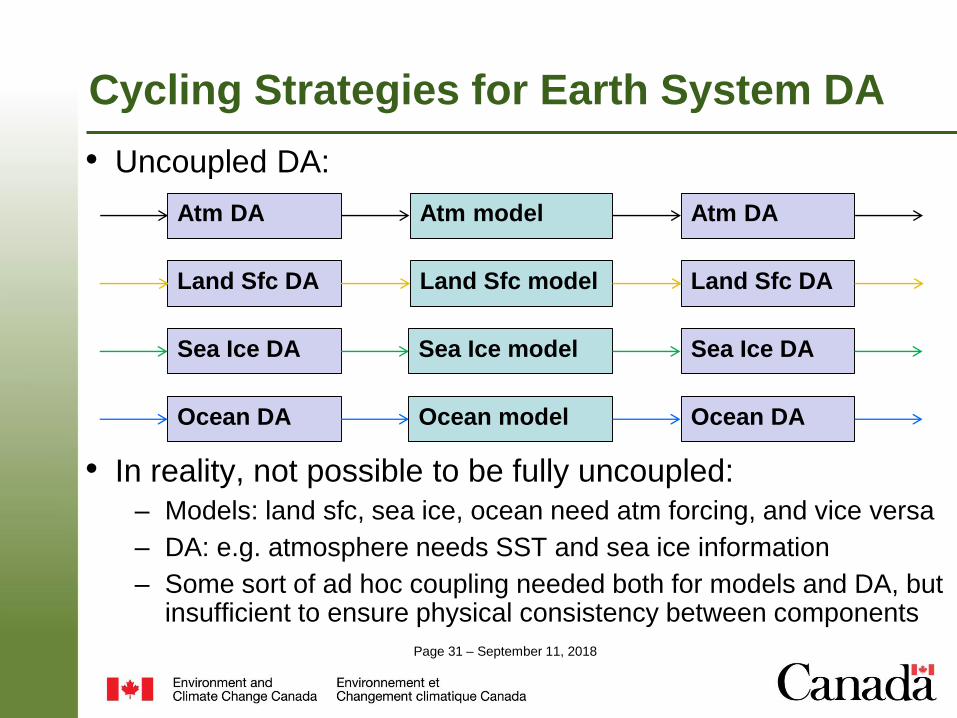
Cycling Strategies for Earth System DA
• Uncoupled DA:
Atm model
Sea Ice DA
Atm DA
Land Sfc DA
Ocean DA
Land Sfc model
Sea Ice model
Ocean model
Sea Ice DA
Atm DA
Land Sfc DA
Ocean DA
• In reality, not possible to be fully uncoupled:
– Models: land sfc, sea ice, ocean need atm forcing, and vice versa
– DA: e.g. atmosphere needs SST and sea ice information
– Some sort of ad hoc coupling needed both for models and DA, but insufficient to ensure physical consistency between components
Page 32 – September 11, 2018
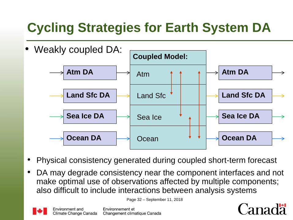
Cycling Strategies for Earth System DA
• Weakly coupled DA:
Sea Ice DA
Atm DA
Land Sfc DA
Ocean DA
Sea Ice DA
Atm DA
Land Sfc DA
Ocean DA
• Physical consistency generated during coupled short-term forecast
• DA may degrade consistency near the component interfaces and not make optimal use of observations affected by multiple components; also difficult to include interactions between analysis systems
Coupled Model:
Atm
Land Sfc
Sea Ice
Ocean
Page 33 – September 11, 2018
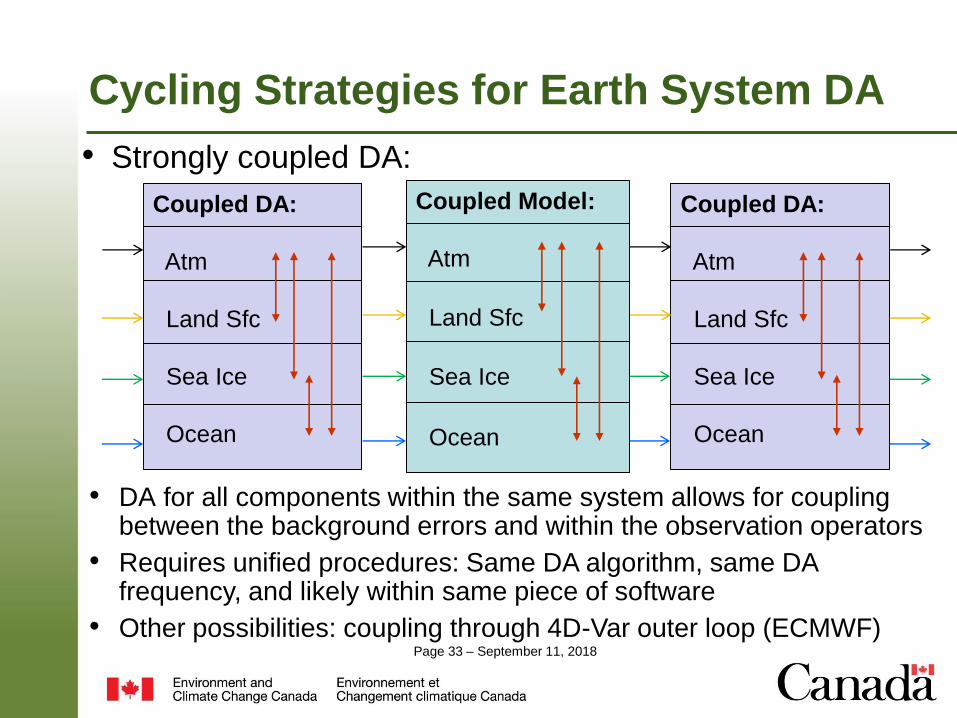
Cycling Strategies for Earth System DA
• Strongly coupled DA:
• DA for all components within the same system allows for coupling between the background errors and within the observation operators
• Requires unified procedures: Same DA algorithm, same DA frequency, and likely within same piece of software
• Other possibilities: coupling through 4D-Var outer loop (ECMWF)
Coupled DA:
Atm
Land Sfc
Sea Ice
Ocean
Coupled Model:
Atm
Land Sfc
Sea Ice
Ocean
Coupled DA:
Atm
Land Sfc
Sea Ice
Ocean
Page 34 – September 11, 2018
Outline
• Motivation: The need for Earth System Data Assimilation
• Methods:
– DA Methods used for NWP, including hybrid methods
– DA Methods for other geophysical components
– Methods for coupled DA
• Examples:
– First attempts at coupled Atmosphere-Ice-Ocean DA at ECCC
• Strategy for Earth System DA at ECCC
Page 35 – September 11, 2018
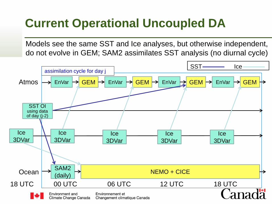
Current Operational Uncoupled DA
EnVarAtmos GEM
SAM2
(daily)Ocean NEMO + CICE
Ice
3DVar
EnVar GEM EnVar GEM EnVar GEM
00 UTC 06 UTC 12 UTC 18 UTC
SST Ice
18 UTC
Ice
3DVarIce
3DVar
Ice
3DVar
assimilation cycle for day j
SST OIusing data of day (j-2)
Ice
3DVar
Models see the same SST and Ice analyses, but otherwise independent,
do not evolve in GEM; SAM2 assimilates SST analysis (no diurnal cycle)
Page 36 – September 11, 2018
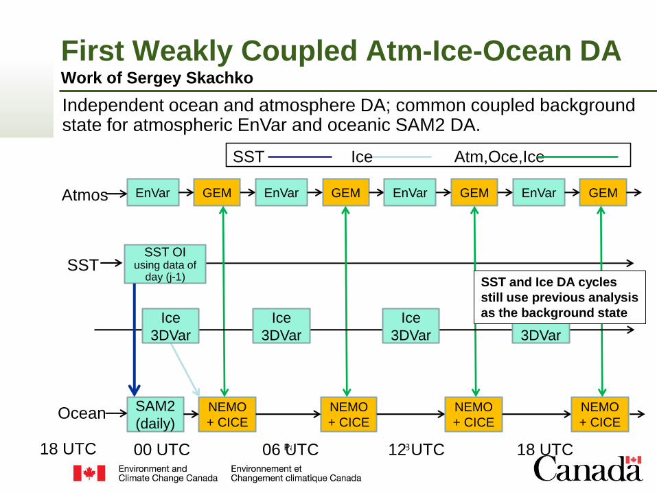
First Weakly Coupled Atm-Ice-Ocean DAWork of Sergey Skachko
EnVarAtmos GEM
SAM2
(daily)Ocean NEMO
+ CICE
EnVar GEM EnVar GEM EnVar GEM
SST
NEMO
+ CICE
NEMO
+ CICE
NEMO
+ CICE
00 UTC 06 UTC 12 UTC 18 UTC
SST Ice Atm,Oce,Ice
18 UTC
SST OIusing data of
day (j-1)
Independent ocean and atmosphere DA; common coupled background state for atmospheric EnVar and oceanic SAM2 DA.
Ice
3DVar
Ice
3DVar
Ice
3DVar
SST and Ice DA cycles
still use previous analysis
as the background stateIce
3DVar
Page 37 – September 11, 2018
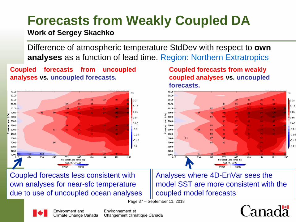
Forecasts from Weakly Coupled DAWork of Sergey Skachko
Difference of atmospheric temperature StdDev with respect to own
analyses as a function of lead time. Region: Northern Extratropics
Coupled forecasts from uncoupled
analyses vs. uncoupled forecasts.
Coupled forecasts from weakly
coupled analyses vs. uncoupled
forecasts.
Coupled forecasts less consistent with
own analyses for near-sfc temperature
due to use of uncoupled ocean analyses
Analyses where 4D-EnVar sees the
model SST are more consistent with the
coupled model forecasts
Page 38 – September 11, 2018
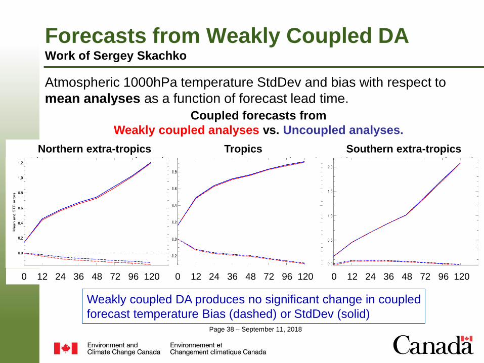
Forecasts from Weakly Coupled DAWork of Sergey Skachko
Atmospheric 1000hPa temperature StdDev and bias with respect to
mean analyses as a function of forecast lead time.
Coupled forecasts from
Weakly coupled analyses vs. Uncoupled analyses.
Weakly coupled DA produces no significant change in coupled
forecast temperature Bias (dashed) or StdDev (solid)
Northern extra-tropics Tropics Southern extra-tropics
0 12 24 36 48 72 96 120 0 12 24 36 48 72 96 120 0 12 24 36 48 72 96 120
Page 39 – September 11, 2018
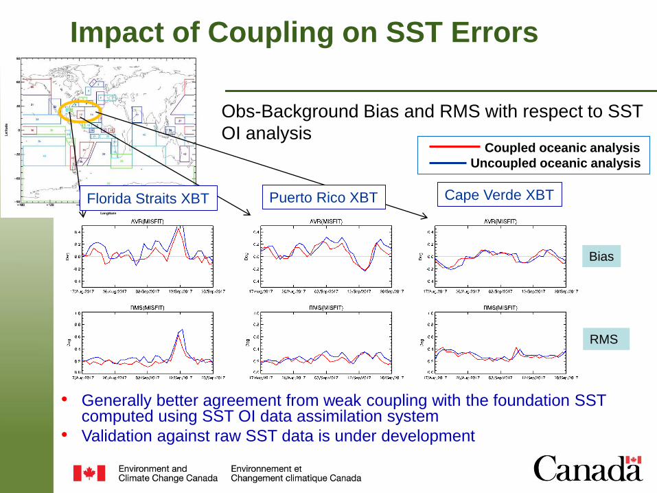
Impact of Coupling on SST Errors
Coupled oceanic analysis
Uncoupled oceanic analysis
• Generally better agreement from weak coupling with the foundation SST computed using SST OI data assimilation system
• Validation against raw SST data is under development
Puerto Rico XBT Cape Verde XBTFlorida Straits XBT
Bias
RMS
Obs-Background Bias and RMS with respect to SST
OI analysis
Page 40 – September 11, 2018
Outline
• Motivation: The need for Earth System Data Assimilation
• Methods:
– DA Methods used for NWP, including hybrid methods
– DA Methods for other geophysical components
– Methods for coupled DA
• Examples:
– First attempts at coupled Atmosphere-Ice-Ocean DA at ECCC
• Strategy for Earth System DA at ECCC
– Use of highly modular common DA software for all components
– Explore scale-dependent combined with system-dependent ensemble covariance localization
Page 41 – September 11, 2018
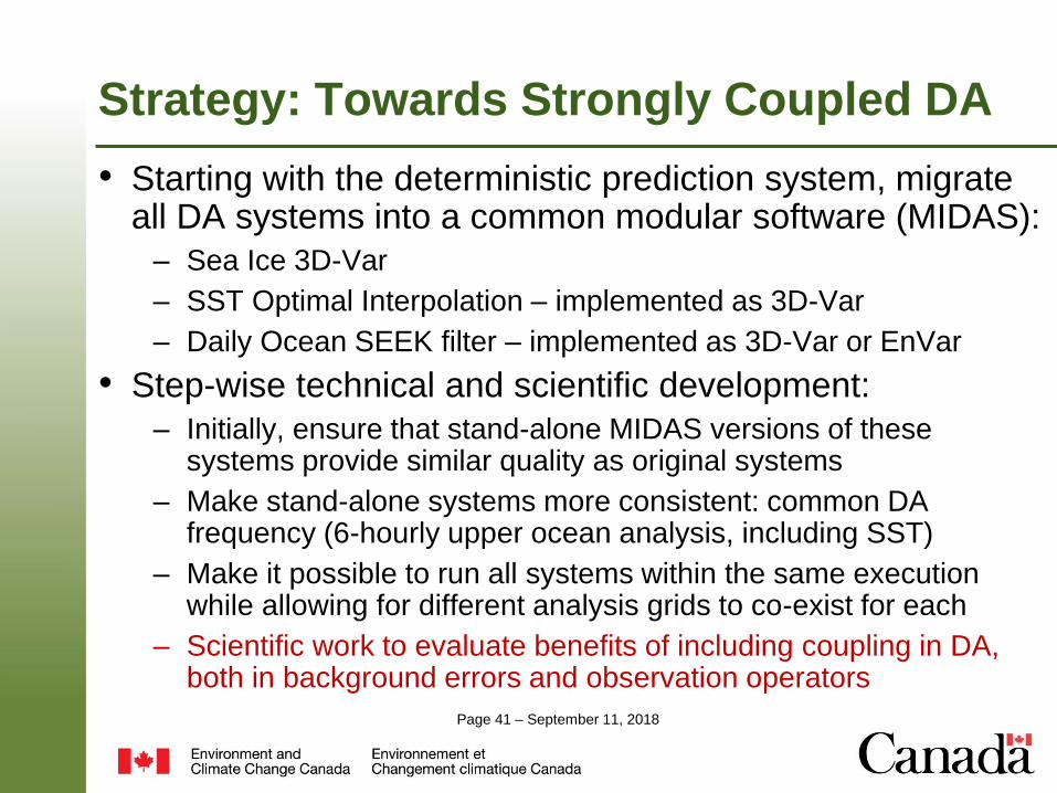
Strategy: Towards Strongly Coupled DA
• Starting with the deterministic prediction system, migrate all DA systems into a common modular software (MIDAS):
– Sea Ice 3D-Var
– SST Optimal Interpolation – implemented as 3D-Var
– Daily Ocean SEEK filter – implemented as 3D-Var or EnVar
• Step-wise technical and scientific development:
– Initially, ensure that stand-alone MIDAS versions of these systems provide similar quality as original systems
– Make stand-alone systems more consistent: common DA frequency (6-hourly upper ocean analysis, including SST)
– Make it possible to run all systems within the same execution while allowing for different analysis grids to co-exist for each
– Scientific work to evaluate benefits of including coupling in DA, both in background errors and observation operators
Page 42 – September 11, 2018
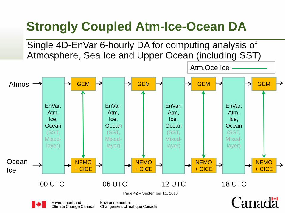
Strongly Coupled Atm-Ice-Ocean DA
EnVar:
Atm,
Ice,
Ocean
(SST,
Mixed-
layer)
Atmos GEM
Ocean
Ice
NEMO
+ CICE
00 UTC 06 UTC 12 UTC 18 UTC
Atm,Oce,Ice
Single 4D-EnVar 6-hourly DA for computing analysis of Atmosphere, Sea Ice and Upper Ocean (including SST)
EnVar:
Atm,
Ice,
Ocean
(SST,
Mixed-
layer)
GEM
NEMO
+ CICE
EnVar:
Atm,
Ice,
Ocean
(SST,
Mixed-
layer)
GEM
NEMO
+ CICE
EnVar:
Atm,
Ice,
Ocean
(SST,
Mixed-
layer)
GEM
NEMO
+ CICE

Page 43 – September 11, 2018
Strategy: Towards Strongly Coupled DA
• Many benefits expected from using highly modular common software (even before coupled DA)
• Modular software components developed for one system can be easily used in another:
– Diffusion-based B matrix developed for sea-ice analysis can be used for SST/Upper-ocean analysis
– Horizontal footprint observation operator developed for sea-ice analysis can be used for atmospheric radiance observations
• By using strongly coupled 4D-EnVar for ensemble mean analysis, may allow transfer of most of the benefit to EnKF
• Lots of interesting science to determine practical methods for estimating and modelling coupled background-error covariances: balance operators, scale/system-dependent ensemble covariance localization and coupling, …
Page 44 – September 11, 2018
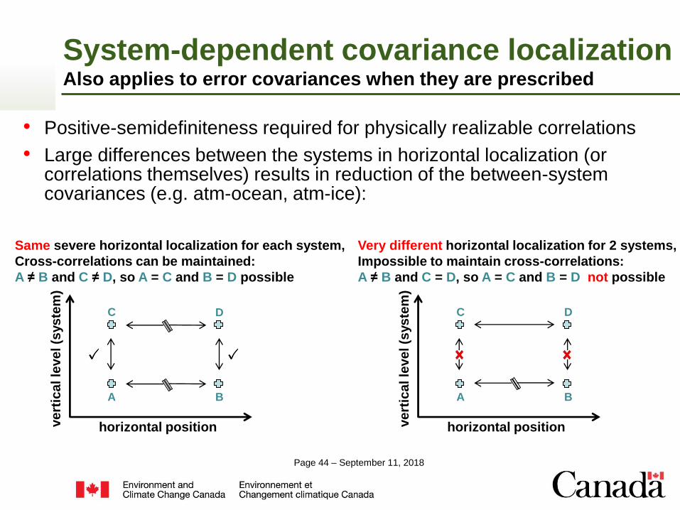
System-dependent covariance localizationAlso applies to error covariances when they are prescribed
• Positive-semidefiniteness required for physically realizable correlations
• Large differences between the systems in horizontal localization (or correlations themselves) results in reduction of the between-system covariances (e.g. atm-ocean, atm-ice):
horizontal positionve
rtic
al le
ve
l (s
ys
tem
)
Same severe horizontal localization for each system,
Cross-correlations can be maintained:
A ≠ B and C ≠ D, so A = C and B = D possible
C D
A B
horizontal positionve
rtic
al le
ve
l (s
ys
tem
)
Very different horizontal localization for 2 systems,
Impossible to maintain cross-correlations:
A ≠ B and C = D, so A = C and B = D not possible
C D
A B
Page 45 – September 11, 2018
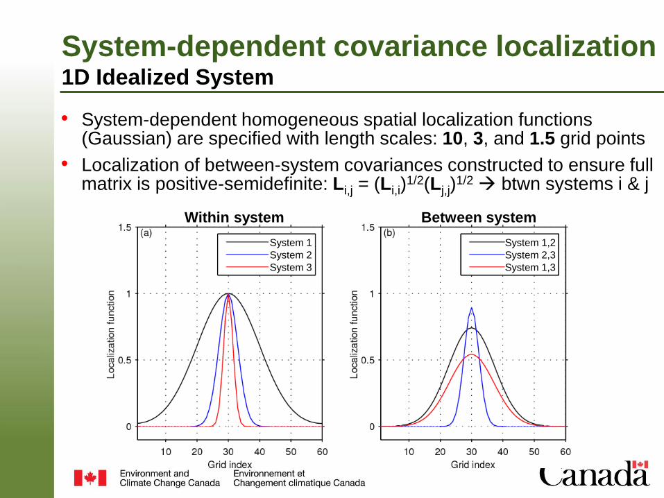
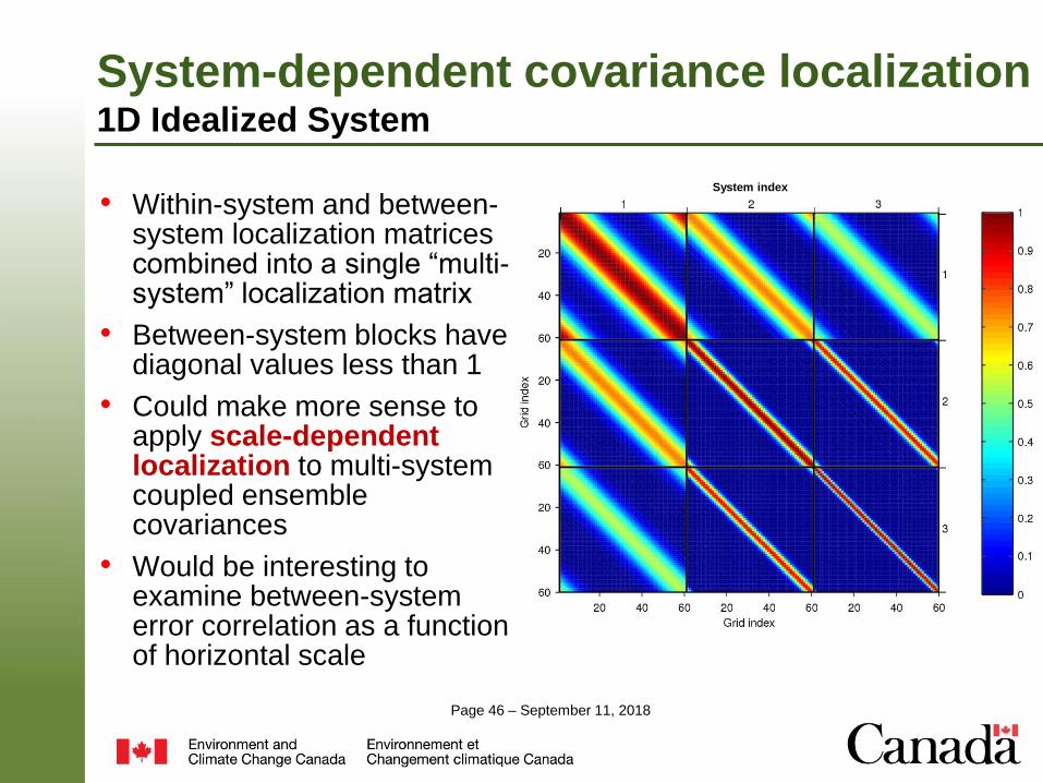
System-dependent covariance localization1D Idealized System
• System-dependent homogeneous spatial localization functions(Gaussian) are specified with length scales: 10, 3, and 1.5 grid points
• Localization of between-system covariances constructed to ensure full matrix is positive-semidefinite: Li,j = (Li,i)
1/2(Lj,j)1/2 btwn systems i & j
Within system Between system
System 1
System 2
System 3
System 1,2
System 2,3
System 1,3
Page 46 – September 11, 2018
System-dependent covariance localization1D Idealized System
• Within-system and between-system localization matricescombined into a single “multi-system” localization matrix
• Between-system blocks have diagonal values less than 1
• Could make more sense to apply scale-dependent localization to multi-system coupled ensemble covariances
• Would be interesting to examine between-system error correlation as a function of horizontal scale
System index
Page 47 – September 11, 2018
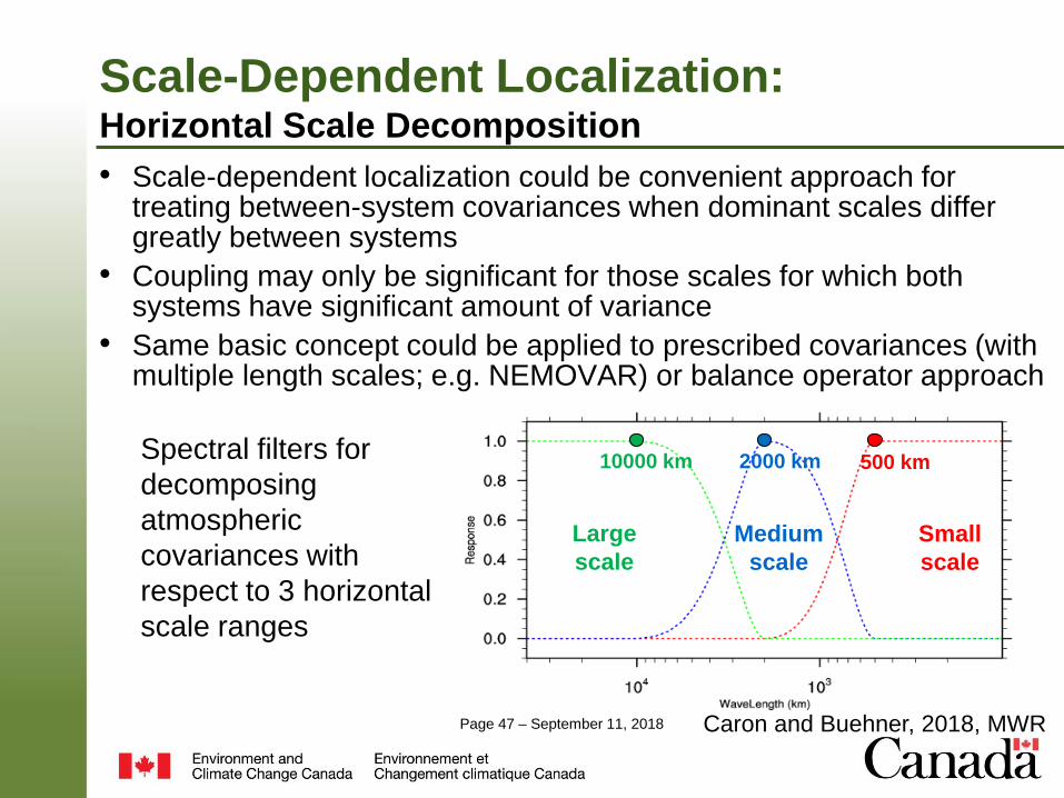
Scale-Dependent Localization: Horizontal Scale Decomposition
Spectral filters for
decomposing
atmospheric
covariances with
respect to 3 horizontal
scale ranges
Large
scale
Medium
scale
Small
scale
2000 km10000 km 500 km
• Scale-dependent localization could be convenient approach for treating between-system covariances when dominant scales differ greatly between systems
• Coupling may only be significant for those scales for which both systems have significant amount of variance
• Same basic concept could be applied to prescribed covariances (with multiple length scales; e.g. NEMOVAR) or balance operator approach
Caron and Buehner, 2018, MWR
Page 48 – September 11, 2018
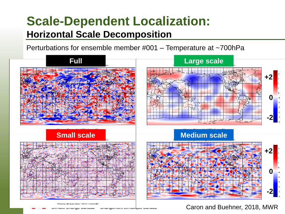
Full Large scale
Small scale Medium scale
Perturbations for ensemble member #001 – Temperature at ~700hPa
0
-2
+2
0
-2
+2
Scale-Dependent Localization: Horizontal Scale Decomposition
Caron and Buehner, 2018, MWR
Page 49 – September 11, 2018
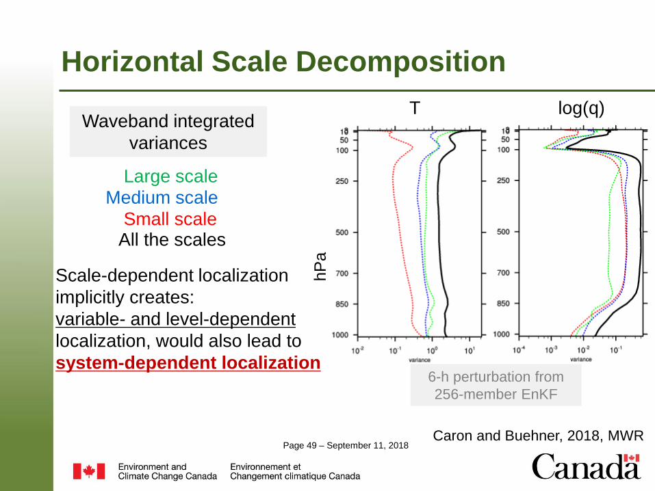
Waveband integrated
variances
Large scaleMedium scale
Small scale
Horizontal Scale Decomposition
6-h perturbation from
256-member EnKF
hP
a
Scale-dependent localization
implicitly creates:
variable- and level-dependent
localization, would also lead to
system-dependent localization
T
All the scales
log(q)
Caron and Buehner, 2018, MWR
Page 50 – September 11, 2018
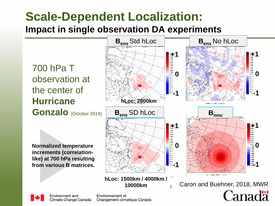
Normalized temperature
increments (correlation-
like) at 700 hPa resulting
from various B matrices.
Scale-Dependent Localization: Impact in single observation DA experiments
Bnmc
Bens No hLocBens Std hLoc
Bens SD hLoc
hLoc: 1500km / 4000km /
10000km
700 hPa T
observation at
the center of
Hurricane
Gonzalo (October 2014)
hLoc: 2800km
0
-1
+1
0
-1
+1
0
-1
+1
0
-1
+1
Caron and Buehner, 2018, MWR
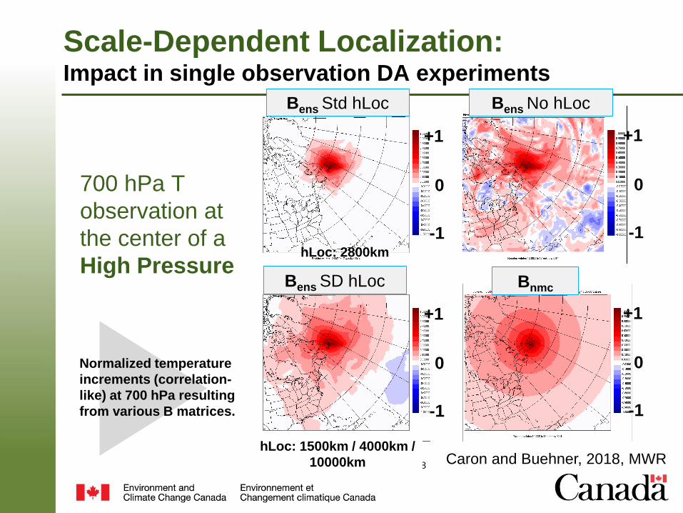
Page 51 – September 11, 2018Caron and Buehner, 2018, MWR
Bens No hLoc
Normalized temperature
increments (correlation-
like) at 700 hPa resulting
from various B matrices.
Scale-Dependent Localization: Impact in single observation DA experiments
Bnmc
Bens Std hLoc
Bens SD hLoc
hLoc: 1500km / 4000km /
10000km
700 hPa T
observation at
the center of a
High PressurehLoc: 2800km
0
-1
+1
0
-1
+1
0
-1
+1
0
-1
+1
Page 52 – September 11, 2018
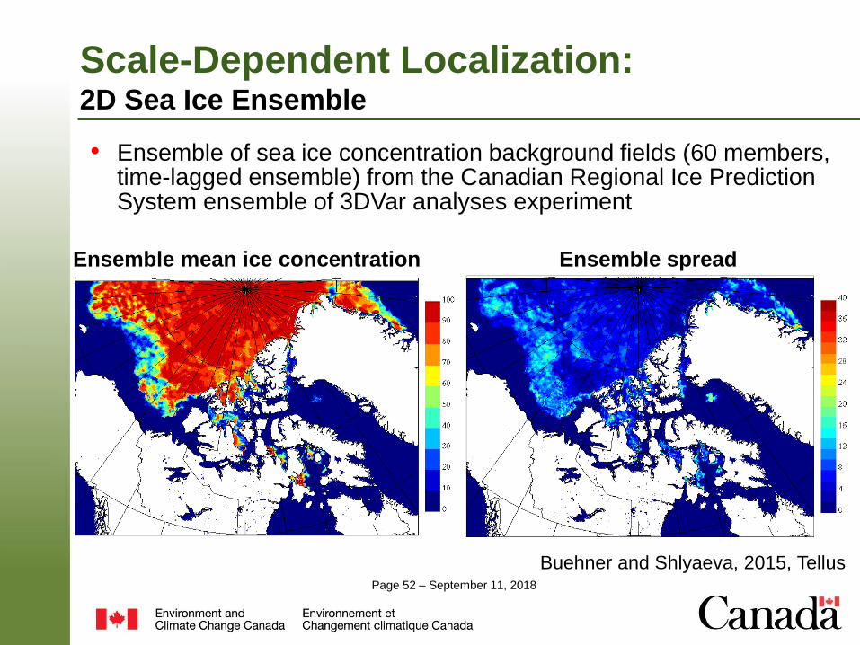
Scale-Dependent Localization:2D Sea Ice Ensemble
• Ensemble of sea ice concentration background fields (60 members, time-lagged ensemble) from the Canadian Regional Ice Prediction System ensemble of 3DVar analyses experiment
Ensemble mean ice concentration Ensemble spread
Buehner and Shlyaeva, 2015, Tellus
Page 53 – September 11, 2018
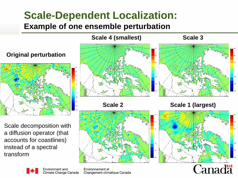
Scale-Dependent Localization: Example of one ensemble perturbation
Original perturbation
Scale 4 (smallest) Scale 3
Scale 2 Scale 1 (largest)
Scale decomposition with
a diffusion operator (that
accounts for coastlines)
instead of a spectral
transform
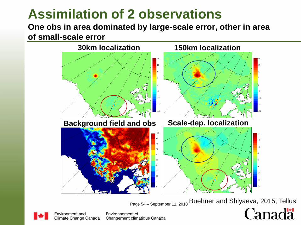
Page 54 – September 11, 2018
Assimilation of 2 observationsOne obs in area dominated by large-scale error, other in area
of small-scale error
Background field and obs
30km localization 150km localization
Scale-dep. localization
Buehner and Shlyaeva, 2015, Tellus
Page 55 – September 11, 2018
Conclusions: Earth System DA
• Many DA systems for NWP moving towards:– Use of large 3D or 4D ensembles with various localization
approaches (e.g. scale-dependent, flow following, etc.)
– Use of increasingly high observation count and spatial resolution
– Use of hybrid approaches to benefit from advantages of each individual method
• Given this complexity of DA for NWP, move towards strongly coupled DA a scientific and technical challenge:
– Requires flexible/modular unified DA software for all systems
– Initial step: use same software for independent systems (forces people to work together and develop flexible/modular code)
• Potential benefits from coupled DA:– More consistent initial conditions for coupled forecasts
– Observations of ice/ocean/land could improve atmosphere
– Account for coupling in observation operators for "coupled" obs